Finite-size corrections to scaling of the magnetization distribution
in the $2d$ $XY$-model at zero temperature

Abstract

The zero-temperature, classical $XY$-model on an $L\times L$ square-lattice is studied by exploring the distribution $\Phi_{L}(y)$ of its centered and normalized magnetization $y$ in the large $L$ limit. An integral representation of the cumulant generating function, known from earlier works, is used for the numerical evaluation of $\Phi_{L}(y)$, and the limit distribution $\Phi_{L\rightarrow\infty}(y)=\Phi_{0}(y)$ is obtained with high precision. The two leading finite-size corrections $\Phi_{L}(y)-\Phi_{0}(y)\approx a_{1}(L)\,\Phi_{1}(y)+a_{2}(L)\,\Phi_{2}(y)$ are also extracted both from numerics and from analytic calculations. We find that the amplitude $a_{1}(L)$ scales as $\ln(L/L_{0})/L^{2}$ and the shape correction function $\Phi_{1}(y)$ can be expressed through the low-order derivatives of the limit distribution, $\Phi_{1}(y)=[\,y\,\Phi_{0}(y)+\Phi^{\prime}_{0}(y)\,]^{\prime}$. The second finite-size correction has an amplitude $a_{2}(L)\propto 1/L^{2}$ and one finds that $a_{2}\,\Phi_{2}(y)\ll a_{1}\,\Phi_{1}(y)$ already for small system size ($L>10$). We illustrate the feasibility of observing the calculated finite-size corrections by performing simulations of the $XY$-model at low temperatures, including $T=0$.

I Introduction

Studies of the scaling properties of fluctuations have played an important role in developing the theory of equilibrium critical phenomena, and they also proved to be instrumental in exploring systems driven far from equilibrium where fluctuations often diverge in the thermodynamic limit. In particular, finding critical exponents through finite-size (FS) scaling has become a standard method for establishing universality classes Fisher -FSS_Num_stat and, furthermore, the shapes of the distribution functions of fluctuations have also been used as hallmarks of universality classes for both equilibrium Bruce -Ex_wide_applic and non-equilibrium systems Racz_et_al -Korniss_et_al .

One of the most studied distribution of critical order-parameter fluctuations is that of the two dimensional classical $XY$ model. The model is important in itself since it serves as a prime example of an equilibrium phase transition with topological order Kosterlitz_Thouless ; Chaikin . Recent interest comes also from a suggestion that its critical magnetization distribution, $P_{L}(m)$, may describe the fluctuations in a remarkable number of diverse far-from-equilibrium steady states. Examples range from the energy-dissipation in turbulence Bramwell_nature ; Aji_Goldenfeld and interface fluctuations in surface evolution Racz_et_al ; Korniss_et_al to electroconvection in liquid crystals Toth_prl , as well as to river-height fluctuations Bramwell_epl . In some of the examples, such as the surface growth problems described by the Edwards-Wilkinson model Edwards_Wilkinson , one can establish a rigorous link to the low-temperature limit (spin-wave approximation) of the $XY$ model. Furthermore, the non-gaussian features of $P_{L}(m)$ such as its exponential and double exponential asymptotes appear to have generic origins Bramwell_PRE2001 ; Bramwell_nat_phys2009 , thus explaining the observed collapse in a remarkable set of experimental and simulation data. In the majority of the examples, however, the experiments or simulations provide data of insufficient accuracy to decide unambiguously about the universality class. Indeed, it is not easy even to observe the changes occurring in $P_{L}(m)$ if the $XY$ model is considered at finite temperatures where the spin-wave approximation breaks down Palma_2005 ; Palma_2006 ; Banks_2005 .

In order to be more confident about universality claims, one would like to be able to examine the distribution functions in more details. A well known and much investigated method of extracting additional information in critical systems such as the zero-temperature $XY$ model is the study of the FS behavior Fisher -FSS_Num_stat . The implication of FS scaling is that the appropriately scaled distribution function has a well defined limit when the system size tends to infinity ($L\to\infty$). A frequently used scaling variable is the centered and normalized magnetization $y=(m-\langle m\rangle)/\sigma_{m}$ where $\sigma_{m}^{2}=\langle m^{2}\rangle-\langle m\rangle^{2}$. This choice of scaling variable eliminates possible divergences in $\langle m\rangle$ and, in general, produces a non-degenerate limit distribution $\Phi_{0}(y)$ Antal_et_al_prl :

$$\lim\limits_{L\to\infty}\Phi_{L}(y)\equiv\lim\limits_{L\to\infty}\sigma_{m}\,P_{L}(\langle m\rangle+\sigma_{m}\,y)=\Phi_{0}(y)\,.$$ (1)

The function $\Phi_{L}(y)$ can be expressed in a compact form for the zero-temperature $XY$ model Archam_1998 . Its large-$L$ limit, $\Phi_{0}(y)$, has been numerically evaluated and compared with simulations and experiments on a variety of systems (see e.g. Bramwell_nature ; Bramwell_PRE2001 ; Bramwell_epl ).

Once the limit distribution is known, one can investigate the approach to $\Phi_{0}(y)$ as the system size increases. As we shall show below, keeping the leading and the next to leading terms, the FS corrections, $\delta\Phi_{L}(y)=\Phi_{L}(y)-\Phi_{0}(y)$, to the limit distribution can be written as

$$\delta\Phi_{L}(y)=a_{1}(L)\,\Phi_{1}(y)+a_{2}(L)\,\Phi_{2}(y)+\mathcal{O}\left(\ln^{2}L/L^{4}\right)\,.$$ (2)

We kept two terms since the asymptotic $L$-dependence of the leading term differs from the next one only by a slowly varying logarithmic factor. Indeed, our calculation yields the amplitudes $a_{i}(L)$ in the following form

$$a_{1}(L)=\frac{\alpha\ln L+\gamma}{L^{2}}=\frac{\alpha\ln(L/L_{0})}{L^{2}}\,,\hskip 11.38092pta_{2}(L)=\frac{\gamma^{\prime}}{L^{2}}\,.$$ (3)

Here, the coefficient $\alpha$ of the logarithmic term can be expressed through the Catalan constant $G$ as $\alpha=3\pi/4G=2.572...\,$. The coefficients of the $1/L^{2}$ terms are $\gamma=-2.803$ (giving $L_{0}=2.973$) and $\gamma^{\prime}=2\pi/3$ (for details, see Sec.III).

A remarkable result about the function $\Phi_{1}(y)$ characterizing the leading shape correction to the limit distribution is that it can be expressed through $\Phi_{0}(y)$ as

$$\Phi_{1}(y)=\left[\,y\,\Phi_{0}(y)+\Phi^{\prime}_{0}(y)\,\right]^{\prime}\,,$$ (4)

where the prime denotes the derivative over $y$. The second scaling function $\Phi_{2}(y)$ is more complex in the sense that it cannot be expressed through a finite sum of the derivatives of the limit distribution. However, it can be calculated efficiently using integral representations as explained in Sec.III [see Eq.(24)] and in Appendix B [see Eq.(52)].

Evaluating the scaling functions $\Phi_{i}(y)$ numerically, one observes that $a_{1}(L)\Phi_{1}(y)\gg a_{2}(L)\Phi_{2}(y)$ already for small systems ($L>10$). This leads to one of the main conclusions of our work, namely that the FS corrections to the limit distribution can be written to an excellent accuracy in the following form

$$\delta\Phi_{L}(y)\approx\alpha\frac{\ln(L/L_{0})}{L^{2}}\,\left[\,y\,\Phi_{0}(y)+\Phi^{\prime}_{0}(y)\,\right]^{\prime}\,.$$ (5)

The above expression can be easily calculated and compared with experiments and simulations using both the scaling of the amplitude and checking the shape of the correction.

It is important to note that $\Phi_{1}(y)$ is uniquely determined by the limit distribution, thus the leading shape correction has the same universality attributes as the limit distribution itself. In renormalization group language, the meaning of the above result is that the eigenfunction corresponding to the direction of slowest approach to the fixed point distribution can be expressed through the limit distribution. A simple and transparent derivation of an analogous result for the case of the central limit theorem can be found in Jona .

In order to show the workings of the method of FS scaling, we carried out Monte Carlo (MC) simulations of the $XY$ model in its low-temperature limit, including its $T=0$-limit. We examined the FS corrections described above for the lattice of size $L=10$, as an illustration, and found close agreement between the theoretical and MC results.

The paper is organized as follows. The $XY$ model and the zero-temperature magnetization distribution is described in Sec.II. Next, the FS corrections are calculated in Sec.III with the technicalities relegated to two Appendices (the direct calculations of the needed cumulants are found in Appendix A, while an integral representation that simplifies the evaluation of finite-volume sums is presented in Appendix B). Finally in Sec.IV, and as an illustration, we have compared the FS results with the MC simulations for a lattice of size $L=10$.

II Probability density of the magnetization for the classical $XY$-model in two-dimensions

The two-dimensional, classical $XY$ model on a square lattice is defined by the Hamiltonian

$$H=-J\sum\limits_{\langle i,j\rangle}\cos(\theta_{i}-\theta_{j})$$ (6)

where the angle variables $\theta_{i}$ describe the orientation of unit vectors in the plane, $J>0$ is the ferromagnetic interaction strength between nearest neighbor vectors on a periodic, $La\times La$ square lattice. From now on we will set $J=1$ and $a=1$, which defines the energy- and length scales in the problem.

The order parameter $m$ whose probability distribution is of our interest is defined as

$$m=\frac{1}{L^{2}}\sum\limits_{i}\cos(\theta_{i}-\bar{\theta})$$ (7)

where $\bar{\theta}$ is the instantaneous average orientation. The probability density function (PDF) of the magnetization, $P_{L}(m)$, has been much studied Archam_1998 ; Bramwell_nature ; Bramwell_epl ; Bramwell_PRE2001 ; Bramwell_nat_phys2009 ; Palma_2005 ; Palma_2006 ; Banks_2005 . Its zero temperature limit ($T\to 0$) has been first calculated Archam_1998 by using the spin-wave approximation $\cos(\theta_{i}-\theta_{j})\approx 1-(\theta_{i}-\theta_{j})^{2}/2$ and summing up the moments series for the PDF.

Another, field-theoretic, approach for obtaining $P_{L}(m)$ is based on evaluating the Fourier transform of the partition function of the system in a loop expansion Palma_2005 . It turns out that the $n$-loops contribution corresponds to the $T^{\,n-1}$ contribution, where $T$ is the system temperature. Correspondingly, the expansion up to one-loop gives exactly the zero-temperature limit of $P_{L}(m)$.

Both of the above methods yield an identical result to leading order. The second method, however, shows explicitly how to compute the higher temperature corrections to $P_{L}(m)$ through an effective, $T$-dependent lattice propagator, $\Gamma=(I+\frac{ikT}{L^{2}}\mathcal{G})^{-1}\mathcal{G}$, where $\mathcal{G}$ is independent of $T$ Cardy , and is defined by its Fourier representation as

$$\mathcal{G}(\mathbf{k})=1/\,\mathbf{\hat{k}}^{2}\hskip 5.69046pt.$$ (8)

Here, the components of the vector $\mathbf{\hat{k}}$ are $\hat{k}_{i}=2\sin(k_{i}/2)$, where $k_{i}=2\pi n_{i}/L$ with $i=1,2$ and $n_{i}\in Z$ such that the lattice momentum $\mathbf{k}$ lies in the first Brillouin zone: $-\pi<k_{i}\leq\pi$.

Hence the PDF at $T=0$ can be obtained by the well known ‘$1/2\,\text{Trace}(\ln)$’ expression of the one-loop result Palma_2005

$$\Phi_{L}(y) =\int_{-\infty}^{\infty}\frac{dq}{2\pi}\hskip 2.84544pt\sqrt{\frac{g_{2}}{2}}\exp{\left(i\sqrt{\frac{g_{2}}{2}}qy\right)}\times\hskip 54.06006pt$$ (9)

$$\exp{\left[-\frac{1}{2}\sum_{\mathbf{k}\neq 0}\left\{\ln{\left(1-\frac{iq}{L^{2}}\mathcal{G}(\mathbf{k})\right)}+\frac{iq}{L^{2}}\mathcal{G}(\mathbf{k})\right\}\right]}$$

where $y$ is the centered and normalized magnetization $y=(m-\langle m\rangle)/\sigma_{m}$, and the coefficient $g_{2}$ is defined as the particular $n=2$ case of the general expression:

$$g_{n}\equiv g_{n}(L)=\sum_{\mathbf{k}\neq 0}\mathcal{G}(\mathbf{k})^{n}/L^{2n}\,.$$ (10)

The PDF in Eq.(9) agrees with the corresponding formula obtained in Bramwell_PRE2001 , (see Eq.(26) therein).

In Fig.1 we plot $\Phi_{L}(y)$ as a function of $y$ using Eq.(9) for different $L$ values. On the right panel, we display a zoom into the region close to the peak of the distribution functions. It can be clearly seen that $\Phi_{L}(y)$ tends towards an asymptotic distribution $\Phi_{0}(y)$ as $L\to\infty$ and, furthermore, one observes that the convergence is fast. Nevertheless, in experiments, the value of $L$ is not known and deviations from $\Phi_{0}(y)$ are observed. They are often explained away as finite-size effects and thus leaving the universality claims not entirely justified. We would like to emphasize that there is information in the FS corrections (shown on Fig.1 around the peak of the PDF) and, by evaluating these corrections, one may refine the reasoning for or against finding a universality class.

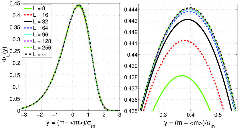
Figure 1: The scaled probability density of the magnetization $\Phi_{L}(y)$, computed numerically using Eq.(9), is displayed for various lattice sizes $L$. The remarkably fast convergence to the limit distribution $\Phi_{0}(y)$ is demonstrated in the left panel while, to illustrate the corrections to the limit distribution, the peak region of the $\Phi_{L}(y)$ is magnified in the right panel.

III Finite-Size Corrections to the Limit Distribution

As explained in Sec.II, the PDF of the magnetization for the $2d$ $XY$-model at $T=0$ is given by the 1-loop analytic expression of Eq.(9), and the numerical evaluation of the $L\to\infty$ limit distribution, $\Phi_{0}(y)$, can be carried out with an excellent precision. The aim of this section is to present the steps of the calculation of the leading and next-to-leading FS corrections to the limit distribution.

We start by expanding the logarithm in the exponential on the r.h.s. of Eq.(9) which allows rewriting the equation in terms of the coefficients $g_{n}$ defined by Eq.(10). After rescaling the integration variable by $\sqrt{g_{2}/2}$, we obtain $\Phi_{L}(y)$ as the following Fourier integral

$$\Phi_{L}(y)=\int\displaylimits_{-\infty}^{\infty}\frac{dk}{2\pi}\exp{\left\{iky-\frac{1}{2}k^{2}+F_{L}(k)\right\}},$$ (11)

where we have defined:

$$F_{L}(k)=\sum_{n\geq 3}\frac{g_{n}}{2n}\left(ik\sqrt{\frac{2}{g_{2}}}\right)^{n}.$$ (12)

The $L$ dependence of the above sum is in the coefficients $g_{n}$ which have a finite non-zero thermodynamic limit $g_{n}(L\to\infty)=g_{n}^{\infty}$ for $n\geq 2$. Thus, in order to compute the FS behavior of $\Phi_{L}(y)$, we shall have to determine the FS corrections to $g_{n}^{\infty}$

$$g_{n}=g_{n}^{\infty}+\delta g_{n}\,.$$ (13)

Assuming that $\delta g_{n}$ is known, we can write $F_{L}(k)$ as

$$F_{L}(k)=F_{0}(k)+\delta F_{1}(k)+\delta F_{2}(k)$$ (14)

where $F_{0}(k)$ is the thermodynamic limit of $F_{L}(k)$:

$$F_{0}(k)=\sum_{n\geq 3}\frac{g_{n}^{\infty}}{2n}\left(ik\sqrt{\frac{2}{g_{2}^{\infty}}}\right)^{n}$$ (15)

and the FS corrections, due to $\delta g_{2}$ and $\delta g_{n}$ for $n\geq 3$, are written separately

$$\delta F_{1}(k) = -\frac{\delta g_{2}}{2g_{2}^{\infty}}\sum_{n\geq 3}\frac{g_{n}^{\infty}}{2}\left(ik\sqrt{\frac{2}{g_{2}^{\infty}}}\right)^{n}\,,\qquad$$ (16)

$$\delta F_{2}(k) = \sum_{n\geq 3}\frac{\delta g_{n}}{2n}\left(ik\sqrt{\frac{2}{g_{2}^{\infty}}}\right)^{n}\,.$$ (17)

The separation of the $\delta g_{2}$ and the $\delta g_{n\geq 3}$ contributions is partly motivated by their $L\to\infty$ asymptotic behaviors. It will be shown in the Appendices that $\delta g_{2}\sim\ln L/L^{2}$ while for $n\geq 3$, $\delta g_{n}\sim 1/L^{2}$. Thus the leading correction comes from $\delta F_{1}(k)$ and the sum in Eq.(16) determines the shape (the functional form) of the leading correction. As it turns out, the same shape correction can be easily separated from the $\delta g_{n}$ contributions for $n\geq 3$. Indeed, for large $n$, one has $\delta g_{n}\sim ng_{n}^{\infty}$, and one can write (cf. Eqs.(32), (38) and (49))

$$\delta g_{n}=\frac{\pi^{2}}{3L^{2}}ng_{n}^{\infty}+\frac{2\pi}{3L^{2}}c_{n}\hskip 5.69046pt,$$ (18)

where the second term is suppressed relative to the first one by a factor $4^{-n}$. Substituting the above split of $\delta g_{n}$ into Eq.(17), one can see the emergence of the same sum as in Eq.(16), and it allows us to write

$$\delta F_{1}(k)+\delta F_{2}(k)=a_{1}(L)\Psi_{1}(k)+a_{2}(L)\Psi_{2}(k)$$ (19)

where the $L$-dependent amplitudes are given by

$$a_{1}(L)=\frac{\delta g_{2}(L)}{2g_{2}^{\infty}}-\frac{\pi^{2}}{3L^{2}}\,,\qquad a_{2}(L)=\frac{2\pi}{3L^{2}}\,,$$ (20)

while the corresponding $L$-independent functions by

$$\Psi_{1}(k) = -\sum_{n\geq 3}\frac{g_{n}^{\infty}}{2}\left(ik\sqrt{\frac{2}{g_{2}^{\infty}}}\right)^{n}=-k\frac{d}{dk}F_{0}(k)\,,\qquad$$

$$\Psi_{2}(k) = \sum_{n\geq 3}\frac{c_{n}}{2n}\left(ik\sqrt{\frac{2}{g_{2}^{\infty}}}\right)^{n}\,.$$ (21)

Integral representations for $F_{0}(k)$ and $\Psi_{2}(k)$ are given in Eqs.(39) and (52), respectively, in Appendix B.

Inserting Eq.(19) into Eq.(11), we obtain the PDF of the $2d$ $XY$-model at zero-temperature, including its leading FS corrections

$$\Phi_{L}(y)=\Phi_{0}(y)+a_{1}(L)\,\Phi_{1}(y)+a_{2}(L)\,\Phi_{2}(y)\hskip 5.69046pt.$$ (22)

Here

$$\Phi_{0}(y)=\int\displaylimits_{-\infty}^{\infty}\frac{dk}{2\pi}\exp{\left\{iky-\frac{k^{2}}{2}+F_{0}(k)\right\}},$$ (23)

and

$$\Phi_{1,2}(y)=\int\displaylimits_{-\infty}^{\infty}\frac{dk}{2\pi}\exp{\left\{iky-\frac{k^{2}}{2}+F_{0}(k)\right\}}\Psi_{1,2}(k)\hskip 2.84544pt.$$ (24)

Since $\Psi_{1}(k)=-kF_{0}^{\prime}(k)$, one can evaluate $\Phi_{1}(y)$ through $\Phi_{0}(y)$ by carrying out the appropriate integrations by part on the r.h.s. of Eq.(24). The outcome is one of the main results of our work, namely a simple expression is obtained for the leading shape correction in terms of the limit distribution (as quoted in Eq.(4)):

$$\Phi_{1}(y)=\left[\,y\,\Phi_{0}(y)+\Phi^{\prime}_{0}(y)\right]^{\prime}.$$ (25)

The second shape correction $\Phi_{2}(y)$ can not be related to $\Phi_{0}(y)$ in such a simple manner but can be readily evaluated using Eqs.(24) and (52) of the Appendix B.

The functions $\Phi_{1}(y)$ and $\Phi_{2}(y)$ are displayed in Fig.2. A general property of these functions is that their 0^th, 1^st and 2^nd moments are zero. This follows from their definition as being corrections to a centered and normalized probability distribution, and can be explicitly verified using their definitions, e.g. Eq.(24).

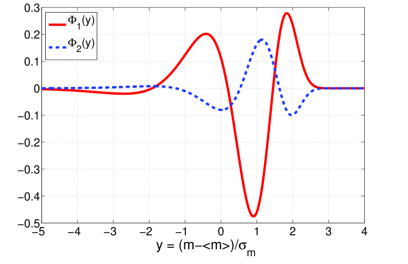
Figure 2: Behavior of the scale independent shape correction functions $\Phi_{1}(y)$ and $\Phi_{2}(y)$.

In order to determine the amplitudes in front of the shape corrections, we have to calculate the FS behavior of $\delta g_{n}$ for $n\geq 2$. This problem is addressed in details, using two distinct methods, in the Appendices A and B. It is found there that the asymptotic $L$-dependence of $\delta g_{2}$ has the form $(C_{1}\ln L+C_{2})/L^{2}$ (cf. Eq.(29)) while $\delta g_{n}$ behaves as $\propto 1/L^{2}$ for $n>2$ (cf. Eqs.(34), (38) and (49)). An important result of these calculations is the amplitude of $\Phi_{1}(y)$ given by

$$a_{1}(L)=\frac{\alpha\ln L+\gamma}{L^{2}}=\frac{\alpha}{L^{2}}\ln\frac{L}{L_{0}}$$ (26)

where the coefficient $\alpha$ is obtained analytically $\alpha=3\pi/(4G)=2.5723613476$ with $G$ being the Catalan constant, while $\gamma=-2.8025632653$ and $L_{0}=2.972759081$ are determined numerically.

The amplitude $a_{1}(L)$ is the second main result of our work since the FS corrections are dominated by the $a_{1}(L)\Phi_{1}(y)$ term. Indeed, $a_{2}(L)/a_{1}(L)$ is small, $0.67$, already for $L=10$ and it decreases with increasing $L$. Furthermore, evaluating $\Phi_{2}(y)$ numerically, one finds that apart from the neighborhood of the zeros of $\Phi_{1}(y)$, the inequality $a_{1}(L)\Phi_{1}(y)\gg a_{2}(L)\Phi_{2}(y)$ holds for $L>10$ as seen in Fig.3.

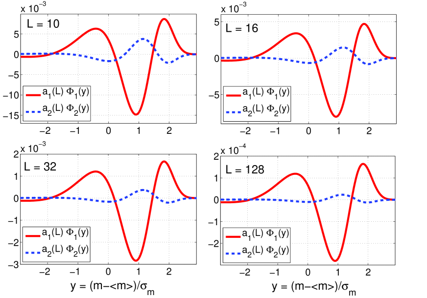
Figure 3: Comparison of the two leading correction terms $a_{1}(L)\Phi_{1}(y)$ and $a_{2}(L)\Phi_{2}(y)$ for $L=10,16,32$ and 128.

It should be mentioned that there is some freedom in separating the two contributions $a_{1}(L)\Phi_{1}(y)$ and $a_{2}(L)\Phi_{2}(y)$ in Eq.(2). One can replace $\Phi_{2}(y)$ by $\Phi_{2}(y)+c\Phi_{1}(y)$ changing simultaneously $\gamma$ to $\gamma-c\gamma^{\prime}$ in $a_{1}(L)$, Eq.(20). Our choice of separating the leading large-$n$ asymptote of $\delta g_{n}$ in Eqs.(18) and (III) leads naturally to a function proportional to $\Phi_{1}(y)$ and also results in a remnant that is small already for small values of $L$. This choice is convenient, since it allows to write the FS correction in a compact form [see Eq.(5)] with a very good accuracy as demonstrated in Fig.4.

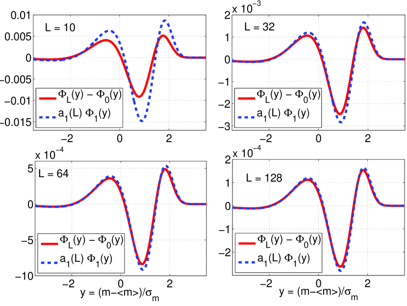
Figure 4: Comparison of the exact FS correction $\Phi_{L}(y)-\Phi_{0}(y)$ with the leading term $a_{1}(L)\Phi_{1}(L)$ given by (25) and (26). Apart from the regions close to the maxima and minima, good agreement can be observed already for small system sizes.

It is remarkable that the dominant correction term $a_{1}(L)\Phi_{1}(y)$ also emerges from a simple assumption about the PDF written in its original variable. Namely, if we assume that one can write $P_{L}(m)=P_{0}(m)+\epsilon(L)P^{\prime\prime}_{0}(m)$ with $\epsilon\to 0$ for $L\to\infty$, we find that $\epsilon(L)=a_{1}(L)\,\sigma_{m}^{2}$. Using then the scaled variable $y$, the expression $\epsilon(L)P^{\prime\prime}_{0}(m)$ becomes $a_{1}(L)\Phi_{1}(y)$.

As discussed above, there are other choices for separating a contribution proportional to $\Phi_{1}(y)$. It should be clear, however, that the freedom is irrelevant when the sum of the two contributions $a_{1}(L)\Phi_{1}(y)+a_{2}(L)\Phi_{2}(y)$ is used. As expected, and as can be seen in Fig.5, the convergence is fastest when the sum of both corrections are used.

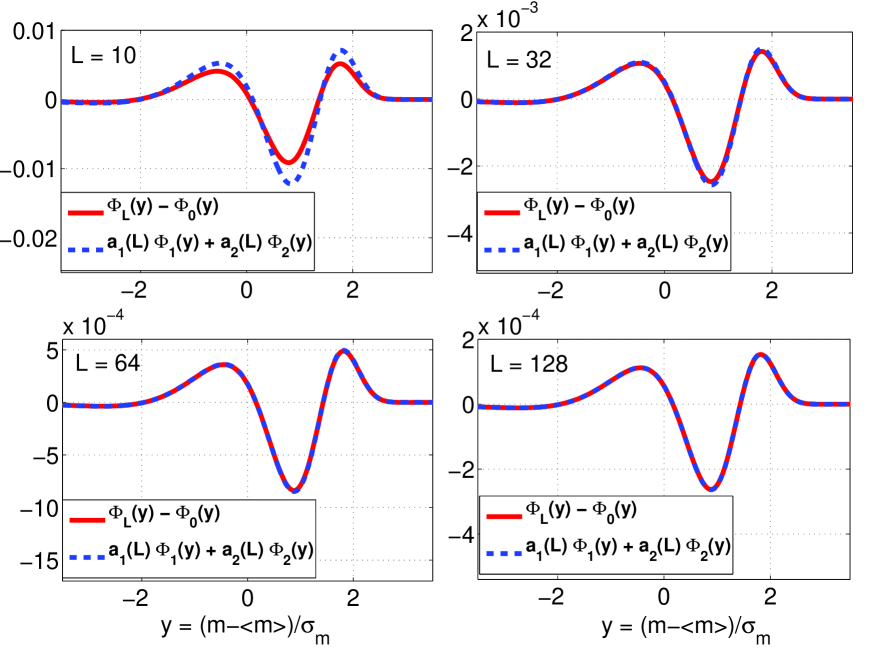
Figure 5: Comparison of the exact FS correction $\Phi_{L}(y)-\Phi_{0}(y)$ with the leading terms $a_{1}(L)\Phi_{1}(L)+a_{2}(L)\Phi_{2}(y)$ for lattice sizes $L=10,32,64$ and 128.

IV Monte Carlo simulations

Here, we briefly demonstrate that the calculated FS corrections can be observed in simulations. It is clear that increasing the system size and improving the statistics by increasing the number of Monte Carlo samples, the leading FS corrections, as seen in Fig.5, will emerge from the analysis. The question is whether the leading corrections we calculated could be seen already in small systems with reasonable simulation effort.

We have thus performed MC simulations on a $2d$ $XY$-model of size $L=10$ and computed $\Phi_{L}(y)$. Since our analytic results Eqs.(22)-(24) pertain to the $T=0$ limit of the system, we made simulations deep in the low $T$ region ($T=0.04$ and $0.02$) using the over-relaxation Metropolis (ORM) algorithm over_relax_MC . In addition, simulations of the $T=0$ limit itself could also be carried out since there the spin-wave approximation applies which yields independent modes with Gaussian action whose simulation is straightforward gaussian .

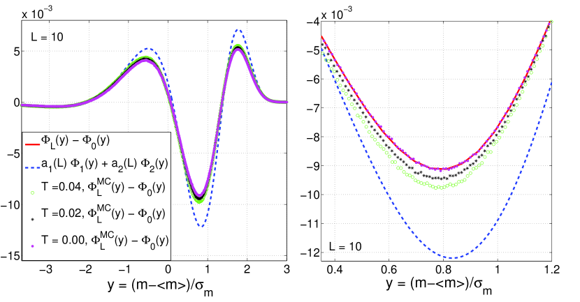
Figure 6: Comparison of the exact FS correction $\Phi_{L}(y)-\Phi_{0}(y)$ (red line) and the leading terms $a_{1}(L)\Phi_{1}(L)+a_{2}(L)\Phi_{2}(y)$ (blue dashed line) with the MC simulations for lattice size $L=10$. The region close to the minimum is magnified in the right panel. It shows that the ORM results approach to $\Phi_{L}(y)-\Phi_{0}(y)$ as $T\rightarrow 0$.

In the simulation using ORM, we typically measured observables using $100\times 10^{9}$ sweeps, and the errors were estimated by using a binning method. On Fig.6, the red line shows the FS corrections to $\Phi_{0}(y)$ displayed as the difference $\Phi_{L=10}(y)-\Phi_{0}(y)$ computed from the integral representation of Eq.(9). It is compared with data obtained by ORM at very low temperatures $T=0.04$ (green circles) and $T=0.02$ (asterisk markers). The magenta points represent the results from the simulation of the Gaussian action at $T=0$. The statistical errors on all the data points displayed are smaller than the point size, which is not surprising for the quoted large number of MC sweeps. From the actual statistical error $\sim 5\times 10^{-5}$ one can find that a relatively small number, $3\times 10^{8}$ sweeps are enough to reach an accuracy $10^{-3}$, one tenth of the maximal FS correction.

As one can see, the simulation temperatures used are small enough for the temperature corrections to be small compared to the FS corrections at $L=10$. It can also be seen that the the sum of the two leading FS correction terms, $a_{1}(L)\Phi_{1}(y)+a_{2}(L)\Phi_{2}(y)$ (blue dashed line) is quite close to the exact result. Of course, $L=10$ is a rather small system to expect full agreement of the calculated leading FS corrections with the full FS correction. Looking at Fig.5, however, one notes that increasing the size of the system by only a factor three would yield a complete domination of the leading FS corrections over the higher order FS corrections.

Thus, we conclude that observing the leading FS corrections is feasible in relatively small systems at relatively small computational coast. Based on this observation, we expect that a meaningful analysis of FS corrections in experimental $XY$ systems is also possible.

V Conclusions

We have computed the leading FS corrections to the PDF of the magnetization of the $2d$ $XY$-model at zero temperature. Two scale-independent functions $\Phi_{1}(y)$ and $\Phi_{2}(y)$ were found with their amplitudes behaving with system size as $a_{1}(L)\sim\alpha\ln(L/L_{0})/L^{2}$ and $a_{2}(L)\sim 1/L^{2}$. The function $\Phi_{1}(y)$ can be expressed through the limit distribution $\Phi_{0}(y)$ and its low-order derivatives. This makes it a candidate for identifying universality features hidden in FS corrections.

The leading and next to leading corrections were found to describe the FS behavior very accurately already for small system size. Thus, as our MC simulations demonstrated, the observation of the calculated FS corrections is possible in model systems. We expect that their experimental observation may also be feasible.

Appendix A Finite-size corrections to $\delta g_{n}$

We begin by deriving the large-$L$ asymptotic expansion for $g_{2}$ defined in Eq.(10). It is convenient to write this equation in the form:

$$g_{2} = \frac{1}{(2\pi)^{4}}\sum_{l,m}^{\prime}\left[l^{2}+m^{2}-\frac{1}{12}\left(\frac{2\pi}{L}\right)^{2}(l^{4}+m^{4})+\cdots\right]^{-2}$$ (27)

$$= g_{2}^{\infty}+\delta g_{2}$$

where the sum goes from $l,m=-L/2+1$, to $L/2$ and prime means that the $l=m=0$ term is left out. The asymptotic value $g_{2}^{\infty}$ is given by

$$g_{2}^{\infty} = \frac{1}{(2\pi)^{4}}\sum_{l,m=-\infty}^{\infty}{}^{\prime}\hskip 8.5359pt\frac{1}{(l^{2}+m^{2})^{2}}=G/(24\pi^{2})$$ (28)

$$\approx 0.0038669$$

where $G$ is the Catalan’s constant.

In the FS correction $\delta g_{2}$, the sum giving the coefficient of $1/L^{2}$ diverges logarithmically with $L$. This leading term is obtained as

$$\delta g_{2} \sim \frac{1}{6(2\pi)^{2}L^{2}}\sum_{l^{2}+m^{2}<L^{2}/4}^{\prime}\hskip 14.22636pt\frac{l^{4}+m^{4}}{(l^{2}+m^{2})^{3}}+\cdots$$ (29)

$$= \frac{1}{6(2\pi)^{2}L^{2}}\int\displaylimits_{1/L}^{1/2}\frac{dr}{r}\int\displaylimits_{0}^{2\pi}d\phi(\sin^{4}{\phi}+\cos^{4}{\phi})+\cdots$$

$$= \frac{1}{16\pi}\frac{\ln{L}}{L^{2}}+\mathcal{O}(L^{-2}).$$

It is worthwhile to mention that the $\ln L/L^{2}$ decay of $\delta g_{2}$ is consistent with the logarithmic FS corrections of some related quantities reported in log_corrections .

The above expression for $\delta g_{2}$ can be generalized to perform a high precision fit of the form:

$$g_{2}(L)=g_{2}^{\infty}+\frac{1}{L^{2}}\left(\frac{1}{16\pi}\ln L+\gamma_{2}\right)\,,$$ (30)

to $g_{2}(L)$ computed numerically using Eq.(10) for a large range of $L$ values footnote2 .

In Fig.7 we have plotted the numerically computed $g_{2}(L)$, as well as the FS scaling expression given by Eq.(30). The value of the parameter $\gamma_{2}=0.003768763799$ was obtained from a high precision fit over system sizes up to $L=10^{9}$. In Appendix B we use a more sophisticated method to obtain an integral representation for $\gamma_{2}$, and found a complete agreement with the value cited above.

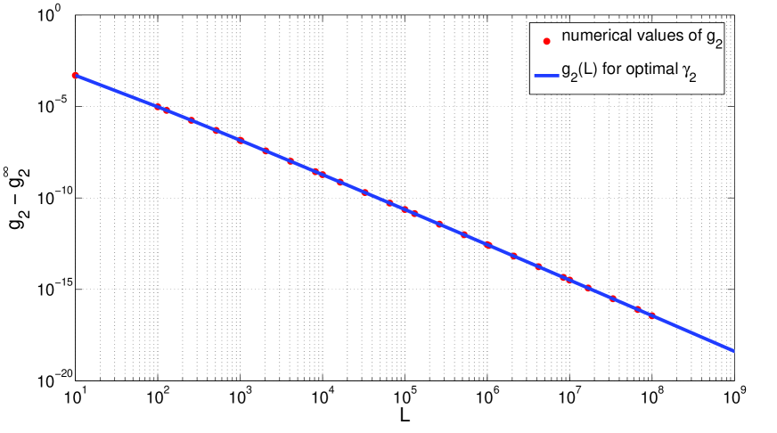
Figure 7: Behavior of $g_{2}(L)$ as a function of lattice size $L$ up to $L=10^{9}$ in logarithmic scale. The red dots correspond to the direct numerical evaluation of Eq.(10) and the blue line corresponds to the analytic expression of Eq.(30) for $\gamma_{2}=0.003768763799$.

Similarly to Eq.(28) the asymptotic value $g_{n}^{\infty}$ is given by

$$g_{n}^{\infty} = \frac{1}{(2\pi)^{2n}}\sum_{l,m=-\infty}^{\infty}{}^{\prime}\hskip 5.69046pt\frac{1}{(l^{2}+m^{2})^{n}}$$ (31)

$$= \frac{4}{(2\pi)^{2n}}\zeta(n)\beta(n)$$

where $\zeta(n)$ and $\beta(n)$ are Riemann’s zeta function and Dirichlet’s beta function, respectively math_func .

For $n\geq 3$ the sum appearing in the $1/L^{2}$ correction term $\delta g_{n}$ converges for $L\to\infty$ hence one can extend the summation to $\pm\infty$ (up to an error decreasing faster than $1/L^{2}$). One has then

$$\frac{\delta g_{n}}{ng_{n}^{\infty}} = \frac{(2\pi)^{2}}{12L^{2}}\frac{\sum_{l,m}^{\prime}\hskip 11.38092pt(l^{4}+m^{4})(l^{2}+m^{2})^{-(n+1)}}{\sum_{l,m}^{\prime}\hskip 11.38092pt(l^{2}+m^{2})^{-n}}$$ (32)

$$= \frac{\pi^{2}}{3L^{2}}\left(1+\frac{U_{n}}{V_{n}}\right)$$

where

$$U_{n} = \sum_{l,m}^{\prime}\hskip 5.69046pt\frac{l^{4}-l^{2}+m^{4}-m^{2}}{(l^{2}+m^{2})^{n+1}}\,\qquad$$

$$V_{n} = \sum_{l,m}^{\prime}\hskip 5.69046pt(l^{2}+m^{2})^{-n}=4\zeta(n)\beta(n)\hskip 5.69046pt.$$ (33)

For large $n$ the dominant terms in these sums come from smallest $|l|$, $|m|$ with non-vanishing contributions. The numerator in $U_{n}$ vanishes for the two shells $(l=\pm 1,m=0)$, $(l=0,m=\pm 1)$ and $(l=\pm 1,m=\pm 1)$. The leading term for large $n$ is coming from $(l=\pm 2,m=0)$, $(l=0,m=\pm 2)$ and is given by $12\cdot 4^{-n}$. Since $V_{n}=4(1+2^{-n}+\ldots)$ one finds that $U_{n}/V_{n}\sim 3\cdot 4^{-n}$. This is a small correction – even for $n=3$ it is just $\approx 0.047$. Hence we have, as stated in Eq.(18)

$$\frac{\delta g_{n}}{ng_{n}^{\infty}}=\frac{\pi^{2}}{3L^{2}}+\frac{1}{L^{2}}\mathcal{O}\left(4^{-n}\right)\,.\qquad n\geq 3$$ (34)

Appendix B Integral representation for leading finite-size corrections

For calculating finite-volume sums for a cubic box of size $L$ in $d$ dimensions in the continuum, like $\sum_{\mathbf{k}}^{\prime}1/(\mathbf{k}^{2})^{n}$, where $\mathbf{k}^{2}=\sum_{i=1}^{d}(2\pi n_{i}/L)^{2}$, it is useful to introduce the function $S(x)$ (see e.g. Has90 ), (related to Jacobi’s theta function) defined as

$$S(x)=\sum_{n=-\infty}^{\infty}\exp\left(-\pi xn^{2}\right).$$ (35)

It satisfies the relation

$$S(x)=\frac{1}{\sqrt{x}}S\left(\frac{1}{x}\right)$$ (36)

which allows to calculate $S(x)$ very precisely by taking only a few terms in the sum, both for $x<1$ and $x>1$. Note that $S(x)=x^{-1/2}(1+2\exp(-\pi/x)+\ldots)$ for $x\to 0$, while $S(x)=1+2\exp(-\pi x)+\ldots$ for large $x$.

As an illustration, it is easy to show that $g_{n}^{\infty}$ given by Eq.(31) has an integral representation

$$g_{n}^{\infty}=\frac{1}{(4\pi)^{n}\Gamma(n)}\int\displaylimits_{0}^{\infty}\mathrm{d}x\,x^{n-1}\left(S^{2}(x)-1\right)\,.$$ (37)

The leading term for $n\to\infty$ is given by the large-$x$ behavior of the integrand. Separating it, one obtains an expression

$$g_{n}^{\infty}=\frac{4}{(2\pi)^{2n}}+ \frac{1}{(4\pi)^{n}\Gamma(n)}\times$$ (38)

$$\int\displaylimits_{0}^{\infty}\mathrm{d}x\,x^{n-1}\left(S^{2}(x)-1-4\mathrm{e}^{-\pi x}\right)$$

which can be evaluated and shown to be in agreement with Eq.(31). With the help of this one can perform the summation in Eq.(15) yielding

$$F_{0}(k)=\int_{0}^{\infty} \frac{\mathrm{d}u}{2u}\left[S^{2}\left(uw\right)-1\right]\times$$ (39)

$$\left\{\mathrm{e}^{iku}-\left(1+iku-\frac{1}{2}k^{2}u^{2}\right)\right\}$$

where $w=4\pi\sqrt{g_{2}^{\infty}/2}$. The Fourier transformation appearing here can be performed efficiently by a fast Fourier transform (FFT).

This technique can be generalized to finite-volume lattice sums by introducing Nie15b

$$Q_{L}(z) = \frac{1}{L}\sum_{l=0}^{L-1}\exp\left(-z\hat{k}_{l}^{2}\right)$$ (40)

$$= \phi_{0}(z)+2\sum_{m=1}^{\infty}\phi_{mL}(z)$$

where $\hat{k}_{l}^{2}=2(1-\cos(2\pi l/L))$, $l=0,\ldots,L-1$, and

$$\phi_{n}(z)=\mathrm{e}^{-2z}I_{n}(2z)$$ (41)

with $I_{n}(z)$ being the modified Bessel function. For large $z$ one has $\phi_{0}(z)\sim 1/\sqrt{4\pi z}$.

For fixed $z$ with increasing $L$ the function $Q_{L}(z)$ approaches $\phi_{0}(z)$ exponentially fast. The approach becomes slower with increasing $z$, but even when the argument increases slower than $L^{2}$ one still has

$$\lim_{L\to\infty}\left(Q_{L}(cL^{\alpha})-\phi_{0}(cL^{\alpha})\right)=0\qquad\text{for }\alpha<2$$ (42)

with the difference decreasing faster than any inverse power of $L$. This is not true for $z\propto L^{2}$, and for this case one obtains another scaling function. Rescaling $Q_{L}(z)$, we introduce the lattice counterpart Nie15b of $S(x)$ by

$$S_{L}(x)=LQ_{L}\left(\frac{xL^{2}}{4\pi}\right)$$ (43)

By expanding Eq.(40) for large $L$ one finds the asymptotic expansion

$$S_{L}(x)=S(x)+\frac{\pi}{3L^{2}}xS^{\prime\prime}(x)+\mathcal{O}\left(\frac{1}{x^{2}L^{4}}\right).$$ (44)

As the error term indicates, the approach to $L=\infty$ is not uniform in $x$.

Using $S_{L}(x)$ one has for $g_{n}=g_{n}(L)$ two integral representations

$$g_{n} = \frac{L^{-2n+2}}{\Gamma(n)}\int_{0}^{\infty}\mathrm{d}z\,z^{n-1}\left[Q_{L}^{2}(z)-\frac{1}{L^{2}}\right]$$ (45)

$$= \frac{1}{(4\pi)^{n}\Gamma(n)}\int_{0}^{\infty}\mathrm{d}x\,x^{n-1}\left[S_{L}^{2}(x)-1\right].$$

We outline below the calculation of $\delta g_{2}$ to $\mathcal{O}\left(1/L^{2}\right)$. Due to the non-uniform convergence for $L\to\infty$ it is useful to split the integration region and write

$$g_{2}(L)=\frac{1}{L^{2}}\int_{0}^{z_{0}} \mathrm{d}z\,z\left[Q^{2}_{L}(z)-\frac{1}{L^{2}}\right]+$$ (46)

$$\frac{1}{(4\pi)^{2}}\int_{x_{0}}^{\infty}\mathrm{d}x\,x\left[S_{L}^{2}(x)-1\right]$$

where $x_{0}=4\pi z_{0}/L^{2}$. Choosing $z_{0}=z_{0}(L)=cL^{2-\epsilon}$ with some fixed small $\epsilon>0$ in the first term one could replace $Q_{L}(z)$ by $\phi_{0}(z)$ up to exponentially small corrections. Similarly, in the second integral one can use the expansion Eq.(44). Note that $z_{0}(L)\to\infty$ and $x_{0}(L)\to 0$ for $L\to\infty$. Using Eq.(44) and neglecting terms vanishing faster than $1/L^{2}$ one obtains

$$\delta g_{2}=\frac{1}{L^{2}}\int_{0}^{z_{0}}\mathrm{d}z\,z\phi_{0}^{2}(z)+\frac{2\pi}{3L^{2}(4\pi)^{2}}\int_{x_{0}}^{\infty}\mathrm{d}x\,x^{2}S(x)S^{\prime\prime}(x)$$ (47)

Separating the asymptotic behavior of the integrands for large $z$, and small $x$, respectively, one obtains the logarithmic contribution $1/(32\pi)\ln(z_{0}/x_{0})=1/(16\pi)\ln L$, and in the remaining terms one can make the substitutions $z_{0}=\infty$ and $x_{0}=0$. Evaluating the corresponding integrals one reproduces the fit result Eq.(30) to all digits (cf. Fig.7).

The leading correction of $\delta g_{n}$ for $n>2$ is simpler and given by the convergent integral

$$\delta g_{n}=\frac{2\pi}{3L^{2}}\frac{1}{(4\pi)^{n}\Gamma(n)}\int_{0}^{\infty}\mathrm{d}x\,x^{n}S(x)S^{\prime\prime}(x)\,,\quad n\geq 3$$ (48)

Separating the large-$x$ term of the integrand one obtains

$$\delta g_{n}= \frac{\pi^{2}}{3L^{2}}\frac{4n}{(2\pi)^{2n}}+\frac{2\pi}{3L^{2}}\frac{1}{(4\pi)^{n}\Gamma(n)}\times$$ (49)

$$\int_{0}^{\infty}\mathrm{d}x\,x^{n}\left[S(x)S^{\prime\prime}(x)-2\pi^{2}\mathrm{e}^{-\pi x}\right]$$

where $n\geq 3$. The leading term has the same form as for $ng_{n}^{\infty}$ (cf. Eq.(38)). Subtracting this way the leading term one can define $c_{n}$ by

$$\delta g_{n}=\frac{\pi^{2}}{3L^{2}}ng_{n}^{\infty}+\frac{2\pi}{3L^{2}}c_{n}$$ (50)

where for $n\geq 3$:

$$c_{n}=\frac{1}{(4\pi)^{n}\Gamma(n)}\int\displaylimits_{0}^{\infty}\mathrm{d}x\,x^{n}S(x)\left(S^{\prime\prime}(x)+\pi S^{\prime}(x)\right).$$ (51)

For large $n$ one has $c_{n}\sim 6\pi n(4\pi)^{-2n}$, i.e. it is suppressed by a factor of $4^{-n}$ compared to $ng_{n}^{\infty}$.

Inserting Eq.(51) into Eq.(III) we obtain an integral representation for $\Psi_{2}(k)$,

$$\Psi_{2}(k)=\frac{w}{2} \int\displaylimits_{0}^{\infty}\mathrm{d}u\,S(uw)\left\{S^{\prime\prime}(uw)+\pi S^{\prime}(uw)\right\}\times$$ (52)

$$\quad\left[\mathrm{e}^{iku}-\left(1+iku-\frac{1}{2}k^{2}u^{2}\right)\right].$$

Using FFT one can evaluate this and finally the corresponding correction $\Phi_{2}(y)$ to the PDF.

References

- (1) M. E. Fisher in Critical Phenomena, Proceedings of the 1970 International School of Physics Enrico Fermi, Course 51, Edited by M. S. Green (Academic, New York, 1971).
- (2) J. L. Cardy, Finite Size Scaling, (North-Holland, Amsterdam, 1988).
- (3) Finite Size Scaling and Numerical Simulation of Statistical Physics, edited by V. Privman (World Scientific, Singapore, 1990).
- (4) A. D. Bruce, J. Phys. C 14, 3667 (1981).
- (5) K. Binder, Z. Phys. B 43, 119 (1981).
- (6) D. Nicolaides, A. D. Bruce, J. Phys. A 21, 233 (1988).
- (7) Examples of wide-ranging applications are: A. D. Bruce and N. B. Wilding, Phys. Rev. Lett. 68, 193 (1992) (liquid-gas transition), D. Nicolaides and R. Ewans Phys. Rev. Lett. 63, 778 (1989) (wetting); N. B. Wilding and P. Niebala, Phys. Rev. E 53, 926 (1996) (tricritical point); M. Müller and N. B. Wilding, Phys. Rev. E 51, 2079 (1995) (polymers); S. L. A. de Queiroz and R. B. Stinchcomb, Phys. Rev. E 64, 036117 (2001) (random-field Ising model); M. M. Tsypin, Phys. Rev. Lett. 73, 2015 (1994) (field theory).
- (8) G. Foltin, K. Oerding, Z. Rácz, R. L. Workman and R. K. P. Zia, Phys. Rev. E 50, R639 (1994); Z. Rácz and M. Plischke, Phys. Rev. E 50, 3530 (1994); E. Marinari, A. Pagnani, G. Parisi, and Z. Rácz, Phys. Rev. E 65, 026136 (2002).
- (9) S. T. Bramwell, P. C. W. Holdsworth, J. -F. Pinton, Nature 396, 552 (1998); R. Labbé, J. -F. Pinton, P. C. W. Holdsworth, Phys. Rev. E 60, R2452 (1999).
- (10) V. Aji and N. Goldenfeld, Phys. Rev. Lett. 86, 1007 (2001)
- (11) S. T. Bramwell et al., Phys. Rev. Lett. 84, 3744 (2000).
- (12) G. Korniss, Z. Toroczkai, M. A. Novotny, and P. A. Rikvold, Phys. Rev. Lett. 84, 1351 (2000); S. Lubeck and P. C. Heger, Phys. Rev. Lett. 90, 230601 (2003); T. Halpin-Healy and G. Palasantzas, EPL 105, 50001 (2014).
- (13) J. M. Kosterlitz and D. J. Thouless, J. Phys. C 6, 1181 (1973).
- (14) P. M. Chaikin and T. C. Lubensky, Principles of Condensed Matter Physics (Cambridge University Press, Cambridge, 1996).
- (15) T. Tóth-Katona and J. Gleeson, Phys. Rev. Lett. 91 264501 (2003); S. Joubaud, A. Petrosyan, S. Ciliberto, and N. B. Garnier, Phys. Rev. Lett. 100, 180601 (2008).
- (16) S. T. Bramwell, T. Fennel, P. C. W. Holdsworth, and B. Portelli, EPL 57, 310 (2002); K. Dahlstedt and H. Jensen, Physica A 348, 596 (2005).
- (17) S. F. Edwards and D. R. Wilkinson, Proc. R. Soc. London, Series A 381, 17 (1982).
- (18) S. T. Bramwell, J.-Y. Fortin, P. C. W. Holdsworth, S. Peysson, J.-F. Pinton, B. Portelli, and M. Sellito, Phys. Rev. E 63, 041106 (2001).
- (19) S. T. Bramwell, Nature Physics 5, 444 (2009).
- (20) G. Mack, G. Palma and L. Vergara, Phys. Rev. E 72, 026119 (2005).
- (21) G. Palma, Phys. Rev. E. 73, 046130 (2006).
- (22) S. T. Banks and S. T. Bramwell, J. Phys. A 38, 5603 (2005).
- (23) T. Antal, M. Droz, G. Györgyi, and Z. Rácz, Phys. Rev. Lett. 87, 240601 (2001); Phys. Rev. E. 65, 046140 (2002).
- (24) P. Archambault, S. T. Bramwell, J.-Y. Fortin, P. C. W. Holdsworth, S. Peysson, J.-F. Pinton, J. Appl. Phys. 83, 7234 (1998).
- (25) G. Jona-Lasinio, Phys. Rep. 352, 439 (2001).
- (26) J. Cardy, Scaling and Renormalization in Statistical Physics, Cambridge University Press (1996).
- (27) M. Creutz, Phys. Rev. D 36, 515 (1987); K. Kanki, D. Loison and K.D. Schotte, Eur. Phys. J. B 44, 309?315 (2005)
- (28) Integrating out the gaussian variables one obtains the analytic expression in Eq.(9).
- (29) R. Kenna and A.C. Irving, Phys. Lett B 351, 273 (1995); W. Janke, Phys. Rev. B 55 (1997); S.G. Chung, Phys. Rev. B 60, 16 (1999)
- (30) Note that in the double sum appearing in (10) the summation over one of the integers can be done analytically, which makes possible to reach large values of .
- (31) See, e.g., I. S. Gradstein and I. M. Ryshik, Table of Integral series and products, seventh edition, Elsevier Academic Press (2007)
- (32) P. Hasenfratz and H. Leutwyler, Nucl. Phys. B 343, 241 (1990).
- (33) F. Niedermayer and P. Weisz, Massless sunset diagrams in finite asymmetric volumes, arXiv:1602.03159 [hep-lat].