The duration distribution of Swift Gamma-Ray Bursts

Abstract

Decades ago two classes of gamma-ray bursts were identified and delineated as having durations shorter and longer than about 2 s. Subsequently indications also supported the existence of a third class. Using maximum likelihood estimation we analyze the duration distribution of 888 Swift BAT bursts observed before October 2015. Fitting three log-normal functions to the duration distribution of the bursts provides a better fit than two log-normal distributions, with 99.9999% significance. Similarly to earlier results, we found that a fourth component is not needed. The relative frequencies of the distribution of the groups are 8% for short, 35% for intermediate and 57% for long bursts which correspond to our previous results. We analyse the redshift distribution for the 269 GRBs of the 888 GRBs with known redshift. We find no evidence for the previously suggested difference between the long and intermediate GRBs’ redshift distribution. The observed redshift distribution of the 20 short GRBs differs with high significance from the distributions of the other groups.

Keywords  Gamma-rays: theory – Gamma rays: observations – Gamma-ray burst: general – Methods: data analysis – Methods: statistical – Cosmology: observations

1 INTRODUCTION

Decades ago (Mazets et al., 1981) and (Norris et al., 1984) suggested that there is a separation in the duration distribution of gamma-ray bursts (GRBs). Today it is widely accepted that the physics of the short and long GRBs are different, and these two kinds of GRBs are different phenomena (Norris et al., 2001; Balázs et al., 2003; Fox et al., 2005; Zhang et al., 2009; Lü et al., 2010).

In the Third BATSE Catalog (Meegan et al., 1996) — using uni- and multi-variate analyses — (Horváth, 1998) and (Mukherjee et al., 1998) found a third type of GRBs. Later several papers (Hakkila et al., 2000; Balastegui et al., 2001; Rajaniemi & Mähönen, 2002; Horváth, 2002; Hakkila et al., 2003; Borgonovo, 2004; Horváth et al., 2006; Chattopadhyay et al., 2007) confirmed the existence of this third (”intermediate” in duration) group in the same database. In the Swift data the intermediate class has also been found (Horváth et al., 2008; Huja et al., 2009). There are also more recent works (Horváth, 2009; Balastegui et al., 2011; de Ugarte Postigo, A. et al., 2011; Lü et al., 2014) in this field.

In the Swift database, the measured redshift distribution for the two groups are also different, for short burst the median is 0.4 (O’Shaughnessy et al., 2008) and for the long ones it is 2.4 (Bagoly et al., 2006).

The paper is organized as follows. Section 2 briefly summarizes the method and fits, Section 3 contains the calculations of the fits and their results, Section 4 contains the comparison of the redshift distributions of the different classes and Section 5 summarizes the conclusions of this paper.

2 THE METHOD

On the Swift web page there are 997 GRBs; 957 of these bursts were catalogued prior to October 2015. Multi-variate analyses have demonstrated that flux and fluence values are also needed for a robust classification. There were 30 GRBs without fluence information and 19 GRBs without peak flux information. Another 20 GRBs are excluded from this analysis because their fluence uncertainties are larger than 50%. Figure 1 shows the $\log T_{90}$ (time to accumulate the central 90% of the burst fluence) distribution of the remaining 888 GRBs.

The maximum likelihood (ML) method assumes that the probability density function of an $x$ observable variable is given in the form of $g(x,p_{1},...,p_{r})$ where $p_{1},...,p_{r}$ are parameters of unknown value. Having $N$ observations on $x$, one can define the likelihood function in the following form:

$$l=\prod_{i=1}^{N}g(x_{i},p_{1},...,p_{r}),\$$ (1)

or in logarithmic form (the logarithmic form is more convenient for calculations):

$$L=\log l=\sum_{i=1}^{N}\log\left(g(x_{i},p_{1},...,p_{r})\right).$$ (2)

The ML procedure maximizes $L$ according to $p_{1},...,p_{r}$. Since the logarithmic function is monotonic, the logarithm reaches its maximum at the same $p_{1},...,p_{r}$ parameter set where $l$ does. The confidence region of the estimated parameters is given by the following formula, where $L_{max}$ is the maximum value of the likelihood function and $L_{0}$ is the likelihood function at the true value of the parameters (Kendall & Stuart, 1976):

$$2(L_{max}-L_{0})\approx\chi^{2}_{r},.$$ (3)

3 LOG-NORMAL FITS OF THE DURATION DISTRIBUTION

Table 1 : The best parameters for the two log-normal fit of the GRB duration distribution.

$$\begin{array}[]{cccc}\hline\cr\vskip 6.0pt\cr&center(logT_{90})&\sigma(logT_{90})&w\\ \vskip 6.0pt\cr\hline\cr\vskip 6.0pt\cr short&0.386&0.484&188.1\\ long&1.700&0.480&699.9\\ \vskip 6.0pt\cr\hline\cr\end{array}$$

Fig. 1 : The duration distribution of Swift BAT bursts.

Similar to our previous work (Horváth, 2002; Horváth et al., 2008), we fit the $T_{90}$ distribution using ML with a superposition of $k$ log-normal components, each of them having two unknown parameters to be fitted with $N=888$ measured points. The choice to use log-normal functions to fit the duration distribution is based on the results of (Balázs et al., 2003; Shahmoradi & Nemiroff, 2015; Zitouni et al., 2015). Our goal is to find the minimum value of $k$ suitable to fit the observed distribution. Assuming a weighted superposition of $k$ log-normal distributions, one has to maximize the following likelihood function:

$$L_{k}=\sum_{i=1}^{N}\log\left(\sum_{m=1}^{k}w_{m}f_{m}(x_{i},\log T_{m},\sigma_{m})\right)$$ (4)

where $w_{m}$ is a weight and $f_{m}$ is a log-normal function with $\log T_{m}$ mean and $\sigma_{m}$ standard deviation having the form of

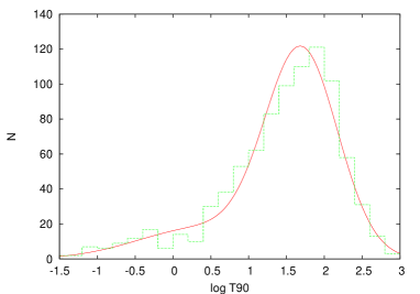
Fig. 2 : Fit with two log-normal component for the duration distribution of BAT bursts.

f_m = 1σm2 π exp( - (x-logTm)22σm2 )

(5)

and due to a normalization condition

$$\sum_{m=1}^{k}w_{m}=N\,.$$ (6)

We used a simple C++ code to find the maximum of $L_{k}$. Assuming only one log-normal component, the fit gives $L_{1max}=4978.88$ but in the case of $k$ = 2 one gets $L_{2max}=5082.246$ with the parameters given in Table 1. The solution is displayed in Fig. 2.

Based on Eq. (3) we can infer whether the addition of a further log-normal component is necessary to significantly improve the fit. We make the null hypothesis that we have already reached the the true value of $k$. Adding a new component, i.e. moving from $k$ to $k+1$, the ML solution of $L_{kmax}$ has changed to $L_{(k+1)max}$, but $L_{0}$ remained the same. In the meantime we increased the number of parameters with 3 ($w_{k+1}$, $logT_{k+1}$ and $\sigma_{(k+1)})$. Applying Eq. (3) on both $L_{kmax}$ and $L_{(k+1)max}$ we get after subtraction

$$2(L_{(k+1)max}-L_{kmax})\approx\chi^{2}_{3}\,.$$ (7)

For $k=1$, $L_{2max}$ is greater than $L_{1max}$ by more than 100, which gives for $\chi^{2}_{3}$ an extremely low probability. It means that the fit with two log-normal distributions is really a better approximation for the duration distribution of GRBs than the fit with one.

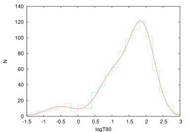
Fig. 3 : Fit with three log-normal components for the duration distribution of BAT bursts.

Thirdly, a three-log-normal fit is made combining three $f_{k}$ functions with eight parameters (three means, three standard deviations and two independent weights). For the best fitted parameters see Table 2. The highest value of the logarithm of the likelihood ($L_{3max}$) is 5098.361. For two log-normal functions the maximum is 5082.246. The maximum has thus improved by 16. Twice this value is 32, which gives us a probability of 0.00006% for the difference between $L_{2max}$ and $L_{3max}$ being only by chance. Therefore, there is a high probability that a third log-normal distribution is needed. In other words, the three-log-normal fit (see Fig. 3) is better and there is a 0.0000006 probability that it was caused only by statistical fluctuation.

Table 2 : The best parameters for the three log-normal fit of the GRB duration distribution.

$$\begin{array}[]{cccc}\hline\cr\vskip 6.0pt\cr&center(logT_{90})&\sigma(logT_{90})&w\\ \vskip 6.0pt\cr\hline\cr\vskip 6.0pt\cr short&-0.508&0.439&68.9\\ long&1.897&0.367&506.3\\ intermediate&1.076&0.448&312.8\\ \vskip 6.0pt\cr\hline\cr\end{array}$$

In one of our previous papers (Horváth et al., 2008), we published a similar analysis on 222 GRBs of the First BAT Catalog. One should compare these results with the results published in that paper. The centers of the distributions change by only a very small amount. In the current analysis, the center of the distribution of the short bursts is at -0.508 (0.311 s) which was previously at -0.473 (0.336 s). For the intermediate ones, the center is at 1.076 which was at 1.107 and for the long bursts at 1.897, which was at 1.903 in our previous analysis. The relative frequencies of the distribution of the groups now are 8% for short, 35% for intermediate and 57% for long bursts (see Table 2). Using a sample four times smaller in 2008 (Horváth et al., 2008), the relative frequencies of the distribution of the groups were 7% for short, 35% for intermediate and 58% for long bursts. Therefore, both analyses give us very similar results. This does not mean that the three-Gaussian is the best approximation for the duration distribution of the GRBs, but strongly suggests that the smaller and the larger sample duration distributions are almost the same. Neither the nature of the GRBs nor the Swift detectors changed during the years.

One should also calculate the likelihood for four log-normal functions. The best logarithm of the ML is 5098.990. It is larger with 0.63 than it was for three log-normal functions. This gives us a low significance (26%), therefore the fourth component is not needed. In Table 3 we summarize the improvement of the likelihood and the corresponding significances.

Table 3 : The improvement of the likelihood and the significances.

$$\begin{array}[]{cccc}\hline\cr\vskip 6.0pt\cr i&L_{imax}&L_{imax}-L_{(i-1)max}&significance\\ \vskip 6.0pt\cr\hline\cr\vskip 6.0pt\cr 2&5082.246&&\\ 3&5098.361&16.1&0.999999\\ 4&5098.99&0.63&0.26\\ \vskip 6.0pt\cr\hline\cr\end{array}$$

4 THE REDSHIFT DISTRIBUTIONS

Among the 888 GRBs there are 269 GRBs which have redshift information. Since the duration distribution of the three groups overlap one cannot be sure to which group does a specific burst belong. However, 2.5 s (0.4 in logarithmic scale) and 31.6 s (1.5 in logarithmic scale) seems to be an approximate border between the short, intermediate and long GBRs. Using these borders, there are 20 short, 79 intermediate and 170 long GRBs. We cut the biggest population, the long burst group, into two parts: shorter than 100 s (91 GRBs) and longer than 100 s (79 GRBs). Figure 4 shows the cumulative distribution of the short, intermediate, long1 and long2 bursts. One can use the Kolmogorov-Smirnov (KS) test to compare the distributions. The redshift distribution of the intermediate, the long1 and the long2 groups do not differ from each other. The probabilities can be seen in Table 4. However, the observed redshift distribution of the short bursts differs from the other three distributions with high significance (more than 99.9 %).

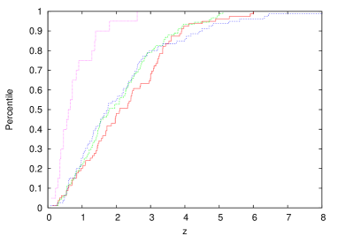
Fig. 4 : The cumulative redshift distribution of the short (pink), intermediate (blue), long1 (green) and long2 (red) bursts.

This latter result is well-known in the literature. For the intermediate bursts, there was a suggestion with a very low significance that the redshift distribution of these bursts are different from the redshift distribution of the long GRBs. Based on the results discussed above, we are not able to confirm this suggestion. The redshift distributions of the long and the intermediate GRBs seem to be very similar.

Table 4 : The KS probabilities assuming the same redshift distribution for the classes.

$$\begin{array}[]{cccc}\hline\cr\vskip 6.0pt\cr p(KS)&intermediate&long1&long2\\ \vskip 6.0pt\cr\hline\cr\vskip 6.0pt\cr short&0.000&0.000&0.000\\ intermediate&&0.90&0.22\\ long1&&&0.21\\ \vskip 6.0pt\cr\hline\cr\end{array}$$

5 CONCLUSIONS

We presented that fitting the duration distribution of 888 Swift BAT GRBs with three log-normal functions is better than the fit using only two. Though this may be the result of statistical fluctuations and maybe there are only two types of GRBs, the probability that the third component is not needed is only 0.00006%. One can compare the parameters of the burst groups with previous results. In (Horváth et al., 2008) the relative frequencies were 7% for short, 35% for intermediate and 58% for long bursts. Now our results show 8% for short, 35% for intermediate and 57% for long ones. The center of the groups are also nearly the same.

We have shown with very high significance that the redshift distribution of the short bursts is different from the redshift distributions of the other (longer) GRBs. However, the redshift distribution of the intermediate GRBs seems to be similar to the redshift distribution of the long GRBs.

Acknowledgements This research was supported by OTKA grant NN111016.

References

- Bagoly et al. (2006) Bagoly, Z., et al. 2006, A&A, 453, 797
- Balastegui et al. (2011) Balastegui, A., Canal, R. & Ruiz-Lapuente, P. 2011, Astronomy Reports, 55, 867
- Balastegui et al. (2001) Balastegui, A., Ruiz-Lapuente, P. & Canal, R. 2001, MNRAS, 328, 283
- Balázs et al. (2003) Balázs, L.G., Bagoly, Z., Horváth, I., Mészáros, A., & Mészáros, P. 2003, A&A, 138, 417
- Borgonovo (2004) Borgonovo, L. 2004, A&A, 418, 487
- Chattopadhyay et al. (2007) Chattopadhyay, T., et al. 2007 ApJ, 667, 1017
- Fox et al. (2005) Fox, D.B., et al. 2005, Nature, 437, 845
- Hakkila et al. (2000) Hakkila, J., et al. 2000, ApJ, 538, 165
- Hakkila et al. (2003) Hakkila, J., et al. 2003, ApJ, 582,320
- Horváth (1998) Horváth, I. 1998, ApJ, 508, 757
- Horváth (2002) Horváth, I. 2002, A&A, 392, 791
- Horváth et al. (2006) Horváth, I., et al. 2006, A&A, 447, 23
- Horváth et al. (2008) Horváth, I., et al. 2008, A&A, 489, L1-L4
- Horváth (2009) Horváth, I. 2009, Ap&SS, 323, 83
- Huja et al. (2009) Huja, D., Mészáros, A., & Řípa, J. 2009, A&A, 504, 67
- Kendall & Stuart (1976) Kendall, M. & Stuart, A. 1976, The Advanced Theory of Statistics (Griffin, London)
- Lü et al. (2010) Lü, H-J., Liang, E-W., Zhang, B-B., & Zhang, B. 2010, ApJ, 725, 1965
- Lü et al. (2014) Lü, H-J., Zhang, B., Liang, E-W., Zhang, B-B., & Sakamoto, T. 2014, MNRAS, 442, 1922
- Mazets et al. (1981) Mazets, E.P., et al. 1981, Ap&SS, 80, 3
- Meegan et al. (1996) Meegan C. A., et al. 1996, ApJS, 106, 65
- Mukherjee et al. (1998) Mukherjee, S., Feigelson, E.D., Babu, G.J., Murtagh, F., Fraley, C. & Raftery, A. 1998, ApJ, 508, 314
- Norris et al. (1984) Norris, J.P., et al. 1984, Nature, 308, 434
- Norris et al. (2001) Norris, J.P., Scargle, J.D., & Bonnell, J.T. 2001, in Gamma-Ray Bursts in the Afterglow Era, Proc. Int. Workshop held in Rome, Italy, eds. E. Costa et al., ESO Astrophysics Symp. (Berlin: Springer), p. 40
- O’Shaughnessy et al. (2008) O’Shaughnessy, R., Belczynski, K., & Kalogera, V. 2008, ApJ, 675, 566
- Shahmoradi & Nemiroff (2015) Shahmoradi, A. & Nemiroff, R. J. 2015, MNRAS, 451, 126
- Rajaniemi & Mähönen (2002) Rajaniemi, H.J., & Mähönen, P. 2002, ApJ, 566, 202
- de Ugarte Postigo, A. et al. (2011) de Ugarte Postigo, A. et al. 2011, A&A, 525, A109
- Zhang et al. (2009) Zhang, B., et al. 2009, ApJ, 703, 1696
- Zitouni et al. (2015) Zitouni, H., Guessoum, N., Azzam, W. J. & Mochkovitch, R. 2015, Ap&SS, 357, 7