AKARI/IRC Near-Infrared Spectral Atlas of Galactic Planetary Nebulae

Abstract

Near-infrared (2.5–5.0$\,\mu$m) low-resolution ($\lambda/\Delta\lambda{\sim}100$) spectra of 72 Galactic planetary nebulae (PNe) were obtained with the Infrared Camera (IRC) in the post-helium phase. The IRC, equipped with a $1^{\prime}{\times}1^{\prime}$ window for spectroscopy of a point source, was capable of obtaining near-infrared spectra in a slit-less mode without any flux loss due to a slit. The spectra show emission features including hydrogen recombination lines and the 3.3–3.5$\,\mu$m hydrocarbon features. The intensity and equivalent width of the emission features were measured by spectral fitting. We made a catalog providing unique information on the investigation of the near-infrared emission of PNe. In this paper, details of the observations and characteristics of the catalog are described.

1 Introduction

Planetary nebulae (PNe) are a late evolutionary stage of low- and intermediate-mass stars (e.g., Schönberner & Blöcker, 1996; Blöcker, 1995). They are surrounded by rich circumstellar material (CSM) ejected during the Asymptotic Giant Branch (AGB) phase (Schönberner et al., 2005). The CSM is eventually incorporated into the interstellar medium and consists of the ingredients for next-generation star-forming activity.

Infrared spectra are rich in CSM emission features. These features can be used to investigate mass, temperature and chemical properties of CSMs (e.g., Pottasch & Bernard-Salas, 2006; Pottasch et al., 1984; Bernard-Salas & Tielens, 2005; Phillips & Márquez-Lugo, 2011). In some PNe, far-infrared emission is dominated by that from dust grains, providing information about the temperature and the total mass of dust grains. Spectroscopic observations in the mid-infrared (${\sim}5$–$40\,\mu$m) have been used to identify dust species (e.g., Volk & Cohen, 1990; Stanghellini et al., 2012). Emission from stochastically heated dust grains also appears in the mid-infrared (Dwek et al., 1997; Draine & Li, 2001). The dust features commonly found are PAHs, MgS, silicate, and some potential cases of SiC. Near-infrared (${\sim}1$–$5\,\mu$m) continuum emission in PNe involves free-free emission, stellar continuum, and hot dust emission. Hydrogen recombination lines are prominent in the near-infrared, such as Brackett-$\alpha$ at 4.051$\,\mu$m. The PAH emission feature appears at 3.3$\,\mu$m (Beintema et al., 1996; Roche et al., 1996; Tokunaga et al., 1991), while there is also emission from aliphatic C−H bonds at around 3.4–3.5$\,\mu$m (Joblin et al., 1996; Sloan et al., 1997).

Infrared space telescopes have been instrumental for PNe observations despite limited spatial resolution. Eliminating the effects of heavy terrestrial atmospheric absorption provides the critical advantage of continuous infrared spectroscopic coverage. Volk & Cohen (1990) investigated 7–23$\,\mu$m low-resolution spectra of 170 Galactic PNe with the Infrared Astronomical Satellite (IRAS). The Short-Wave Spectrometer (SWS) and the Long-Wave Spectrometer (LWS) on-board the Infrared Space Observatory (ISO) cover 2.5–45 and 45–197$\,\mu$m. A number of emission lines have been identified and the physical conditions of circumstellar nebulae have been investigated (e.g., Pottasch & Bernard-Salas, 2006; Bernard-Salas & Tielens, 2005). The Infrared Spectrograph (IRS) on-board the Spitzer space telescope covers 5.5–37$\,\mu$m. Stanghellini et al. (2012) obtained 157 spectra of compact Galactic PNe and investigated their dust emission. Spectra of PNe in the Magellanic Clouds were also obtained with the IRS (Stanghellini & Haywood, 2010; Bernard-Salas et al., 2009, 2008) thanks to its high sensitivity. The ISO/SWS had obtained 2.5–5.0$\,\mu$m spectra of Galactic PNe. About 85 spectra of Galactic PNe are available in Sloan et al. (2003). However, only a few PNe have spectra with a sufficient signal-to-noise ratio at 2.5–5.0$\,\mu$m to investigate weak features such as the 3.4–3.5$\,\mu$m aliphatic emission. The Infrared Camera (IRC) on-board AKARI satellite, for the first time, provides near-infrared (2.5–5.0$\,\mu$m) spectroscopy with a sensitivity of a few mJy (Onaka et al., 2007).

The present paper reports near-infrared spectroscopy with the AKARI/IRC. Observations were carried out as part of an Open Time Program for the post-helium phase, “Near-Infrared Spectroscopy of Planetary Nebulae” (PNSPC). Near-infrared spectra of 72 PNe were obtained. The data were compiled as a near-infrared spectral catalog. In this paper, we describe details of the observations and the characteristics of the catalog. Detailed information about the observations is given in Section 2. Section 3 describes the reduction procedures and the method to extract the spectra. The characteristics of the retrieved spectra and the format of the compiled catalog are presented in Section 4. The quality of the IRC spectra and the statistical properties of the catalog are discussed in comparison with the observations by other facilities in Section 5. We summarize the paper in Section 6.

2 Observations

2.1 Target Selection

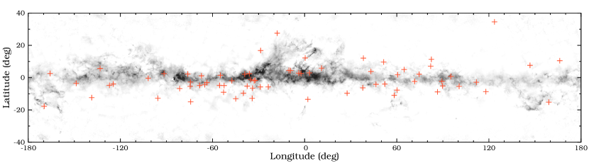
Figure 1: Distribution of the observed planetary nebulae (the crosses) overlaid on an extinction map in the Galactic coordinates created from the DSS (Dobashi et al., 2005a). The gray scale indicates extinction at the $V$-band from 0.1 to 5 mag.

The observed targets were selected from the Strasbourg-ESO Catalogue of Galactic Planetary Nebulae (Acker et al., 1992), taking into account their NIR magnitude and angular size. The spectroscopic sensitivity of the IRC is a few mJy in the range of 2–5$\,\mu$m, while the saturation limit is about 10 Jy. With these limits taken into account, objects whose $K$-band magnitude is between 5 and 13 were selected as targets for this program. The observations were carried out with the $1\arcmin{\times}1\arcmin$ Np-window (see Section 2.2 and Onaka et al., 2007) in the slit-less mode. Therefore, compact objects were preferred to avoid degrading the spectral resolution. The candidate list was then narrowed to objects whose radius in the optical was smaller than $5\arcsec$, comparable to the full width half maximum of the IRC point spread function $({\sim}3\arcsec)$, to exclude apparently large objects. Finally, 72 objects were selected and their spectra were successfully obtained. Figure 1 shows the distribution of the targets in the Galactic coordinates. The PNG ID, the AKARI observation ID, and the coordinates of the PNSPC samples are listed in Table 1. Table AKARI/IRC Near-Infrared Spectral Atlas of Galactic Planetary Nebulae summarizes miscellaneous information of the objects, including the optical (the $V$-band) and infrared (the 2MASS $K_{s}$-band) magnitudes.

The target selection method was independent of the chemistry and dust compositions of the circumstellar nebula. The catalog is not considered to be biased, in terms of chemical abundance and the chemistry of dust. However, the objects were selected based on their sizes. Since PNe expand as they evolve, the selection could be biased toward young PNe. The potential biases of the PNSPC samples are discussed in detail in Section 5.

2.2 Instruments

Although the AKARI/IRC has three channels (Onaka et al., 2007), only the NIR channel was available during the post-helium phase. The field of view of the NIR channel consists of four parts: the N/Nc-window, the Ns-slit, the Np-window, and the Nh-slit (see, Figure 3 in Onaka et al., 2007). The observations were performed with the Np-window, which was designed for point source, slit-less spectroscopy. Spectroscopy with the Np-window allows us to collect all of the flux from an object. The present spectroscopy was carried out with the grism, providing 2.5–5.0$\,\mu$m spectra with the spectral resolution of $\lambda/\Delta\lambda{\sim}100$, for point sources (${\lesssim}3^{\prime\prime}$). The spectral resolution was degraded for extended objects.

The observations were carried out with the observation template IRCZ4. This mode consists of three sequences: the first set is four spectroscopic images, the second set is a broad band image, and the final set is another sequence of four spectroscopic images. Thus, each pointing observation involves eight frames for spectroscopy and one frame for broad-band imaging. Every frame consists of short (4.58 sec) and long (44.41 sec) exposure images. Due to the short integration time, the typical signal-to-noise ratio of the short exposure images is worse than that of the long exposure images. In general, we used only the long exposure images. The short exposure images were used only for cases when the long exposure image showed saturated pixels.

Each object was observed either once, or twice. Thus, there were eight or sixteen frames for each object. However, some frames were not usable due to cosmic rays or unstable pointing during the exposure. The net integration time thus depends on the target, listed in the sixth column of Table 1.

Table 1: Summary of Observations

PN G	Obs. ID	RA (J2000)	DEC (J2000)	$N$(a)	$t_{\rm int}$(b)	FWHM	Flags
		$hh{:}mm{:}ss$	$dd{:}mm{:}ss$		${\rm sec.}$	${\rm\mu m}$	$\mathcal{S}$(c)	$\mathcal{D}$(d)	$\mathcal{C}$(e)
000.3${+}$12.2	$3460107$	$17:01:33.6$	$-21:49:33.5$	$17$	$754.97$	$0.045$	N	N	N
002.0${-}$13.4	$3460003$	$18:45:50.7$	$-33:20:35.0$	$16$	$710.56$	$0.040$	N	Y	N
003.1${+}$02.9	$3460005$	$17:41:52.8$	$-24:42:07.7$	$9$	$399.69$	$0.045$	N	Y	Y
011.0${+}$05.8	$3460012$	$17:48:19.8$	$-16:28:44.0$	$18$	$799.38$	$0.035$	N	N	N
027.6${-}$09.6	$3460016$	$19:16:28.3$	$-09:02:37.0$	$9$	$399.69$	$0.040$	N	Y	N
037.8${-}$06.3	$3460019$	$19:22:56.9$	$+01:30:48.0$	$17$	$754.97$	$0.035$	N	Y	N
038.2${+}$12.0	$3460020$	$18:17:34.0$	$+10:09:05.0$	$9$	$399.69$	$0.040$	N	N	N
043.1${+}$03.8	$3460093$	$18:56:33.6$	$+10:52:12.0$	$9$	$399.69$	$0.035$	N	Y	Y
046.4${-}$04.1	$3460021$	$19:31:16.4$	$+10:03:21.7$	$9$	$399.69$	$0.040$	N	Y	Y
051.4${+}$09.6	$3460022$	$18:49:47.6$	$+20:50:39.5$	$17$	$754.97$	$0.040$	N	N	N
052.2${-}$04.0	$3460094$	$19:42:18.7$	$+15:09:09.0$	$18$	$799.38$	$0.035$	N	Y	N
058.3${-}$10.9	$3460023$	$20:20:08.8$	$+16:43:54.0$	$18$	$799.38$	$0.040$	N	N	N
060.1${-}$07.7	$3460024$	$20:12:42.9$	$+19:59:23.0$	$14$	$621.74$	$0.048$	N	Y	N
060.5${+}$01.8	$3460025$	$19:38:08.4$	$+25:15:42.0$	$18$	$799.38$	$0.035$	N	Y	N
064.7${+}$05.0	$3460026$	$19:34:45.3$	$+30:30:59.2$	$17$	$\phantom{0}77.86$	$0.048$	Y	N	N
071.6${-}$02.3	$3460027$	$20:21:03.8$	$+32:29:24.0$	$18$	$799.38$	$0.035$	N	N	N
074.5${+}$02.1	$3460028$	$20:10:52.5$	$+37:24:41.0$	$18$	$799.38$	$0.040$	N	N	N
082.1${+}$07.0	$3460029$	$20:10:23.7$	$+46:27:39.0$	$18$	$799.38$	$0.045$	N	Y	N
082.5${+}$11.3	$3460030$	$19:49:46.6$	$+48:57:40.0$	$9$	$399.69$	$0.035$	N	Y	N
086.5${-}$08.8	$3460114$	$21:33:08.3$	$+39:38:09.7$	$18$	$799.38$	$0.045$	N	Y	N
089.3${-}$02.2	$3460031$	$21:19:07.2$	$+46:18:48.0$	$18$	$799.38$	$0.038$	N	Y	N
089.8${-}$05.1	$3460032$	$21:32:31.0$	$+44:35:47.7$	$18$	$799.38$	$0.035$	N	N	N
095.2${+}$00.7	$3460033$	$21:31:50.2$	$+52:33:52.0$	$18$	$799.38$	$0.042$	N	Y	N
100.6${-}$05.4	$3460034$	$22:23:55.7$	$+50:58:00.0$	$18$	$799.38$	$0.035$	N	N	N
111.8${-}$02.8	$3460035$	$23:26:14.9$	$+58:10:53.0$	$8$	$355.28$	$0.038$	N	N	N
118.0${-}$08.6	$3460096$	$00:18:42.2$	$+53:52:20.0$	$16$	$710.56$	$0.035$	N	Y	N
123.6${+}$34.5	$3460115$	$12:33:06.8$	$+82:33:50.1$	$18$	$799.38$	$0.065$	N	Y	N
146.7${+}$07.6	$3460097$	$04:25:50.8$	$+60:07:12.7$	$18$	$799.38$	$0.035$	N	N	N
159.0${-}$15.1	$3460098$	$03:47:33.0$	$+35:02:48.9$	$9$	$399.69$	$0.045$	N	Y	N
166.1${+}$10.4	$3460116$	$05:56:23.9$	$+46:06:17.2$	$18$	$799.38$	$0.050$	N	N	N
190.3${-}$17.7	$3460099$	$05:05:34.3$	$+10:42:23.8$	$9$	$399.69$	$0.045$	N	N	N
194.2${+}$02.5	$3460117$	$06:25:57.2$	$+17:47:27.3$	$18$	$799.38$	$0.045$	N	N	N
211.2${-}$03.5	$3460036$	$06:35:45.1$	$+00:05:38.0$	$16$	$710.56$	$0.035$	N	N	N
221.3${-}$12.3	$3460118$	$06:21:42.7$	$-12:59:14.0$	$15$	$666.15$	$0.046$	N	N	N
226.7${+}$05.6	$3460100$	$07:37:18.9$	$-09:38:50.0$	$17$	$754.97$	$0.040$	N	Y	N
232.8${-}$04.7	$3460037$	$07:11:16.7$	$-19:51:04.0$	$14$	$621.74$	$0.035$	N	N	N
235.3${-}$03.9	$3460038$	$07:19:21.5$	$-21:43:54.3$	$17$	$754.97$	$0.035$	N	N	N
258.1${-}$00.3	$3460039$	$08:28:28.0$	$-39:23:40.0$	$17$	$754.97$	$0.042$	N	N	N
264.4${-}$12.7	$3460040$	$07:47:20.0$	$-51:15:03.4$	$17$	$754.97$	$0.035$	N	Y	N
268.4${+}$02.4	$3460042$	$09:16:09.6$	$-45:28:42.8$	$18$	$799.38$	$0.038$	N	N	N
278.6${-}$06.7	$3460101$	$09:19:27.5$	$-59:12:00.3$	$18$	$799.38$	$0.040$	N	Y	N
283.8${+}$02.2	$3460044$	$10:31:33.4$	$-55:20:50.5$	$16$	$710.56$	$0.045$	N	Y	N
285.4${-}$05.3	$3460120$	$10:09:20.8$	$-62:36:48.5$	$18$	$799.38$	$0.050$	N	Y	N
285.6${-}$02.7	$3460045$	$10:23:09.1$	$-60:32:42.3$	$17$	$754.97$	$0.042$	N	Y	N
285.7${-}$14.9	$3460121$	$09:07:06.3$	$-69:56:30.6$	$17$	$754.97$	$0.060$	N	N	N
291.6${-}$04.8	$3460046$	$11:00:20.0$	$-65:14:57.8$	$18$	$799.38$	$0.038$	N	Y	N
292.8${+}$01.1	$3460102$	$11:28:47.4$	$-60:06:37.3$	$18$	$799.38$	$0.042$	N	Y	N
294.9${-}$04.3	$3460047$	$11:31:45.4$	$-65:58:13.7$	$18$	$799.38$	$0.035$	N	N	N
296.3${-}$03.0	$3460048$	$11:48:38.2$	$-65:08:37.3$	$15$	$666.15$	$0.035$	N	N	N
304.5${-}$04.8	$3460051$	$13:08:47.3$	$-67:38:37.6$	$16$	$710.56$	$0.038$	N	Y	N
305.1${+}$01.4	$3460122$	$13:09:36.4$	$-61:19:35.6$	$18$	$\phantom{0}82.44$	$0.050$	Y	N	N
307.2${-}$09.0	$3460052$	$13:45:22.4$	$-71:28:55.7$	$18$	$799.38$	$0.035$	N	Y	Y
307.5${-}$04.9	$3460053$	$13:39:35.1$	$-67:22:51.7$	$18$	$799.38$	$0.040$	N	Y	Y
312.6${-}$01.8	$3460123$	$14:18:43.3$	$-63:07:10.1$	$16$	$710.56$	$0.056$	N	Y	N
315.1${-}$13.0	$3460054$	$15:37:11.2$	$-71:54:52.9$	$18$	$\phantom{0}82.44$	$0.042$	Y	N	N
320.1${-}$09.6	$3460103$	$15:56:01.7$	$-66:09:09.2$	$16$	$710.56$	$0.045$	N	Y	N
320.9${+}$02.0	$3460056$	$15:05:59.2$	$-55:59:16.5$	$9$	$399.69$	$0.042$	N	Y	N
322.5${-}$05.2	$3460060$	$15:47:41.2$	$-61:13:05.6$	$16$	$710.56$	$0.092$	N	Y	Y
323.9${+}$02.4	$3460061$	$15:22:19.4$	$-54:08:13.1$	$9$	$399.69$	$0.045$	N	Y	N
324.8${-}$01.1	$3460062$	$15:41:58.8$	$-56:36:25.6$	$8$	$355.28$	$0.036$	N	Y	Y
325.8${-}$12.8	$3460063$	$16:54:35.2$	$-64:14:28.4$	$16$	$710.56$	$0.035$	N	Y	N
326.0${-}$06.5	$3460064$	$16:15:42.3$	$-59:54:01.0$	$14$	$621.74$	$0.035$	N	Y	Y
327.1${-}$01.8	$3460065$	$15:58:08.1$	$-55:41:50.3$	$9$	$399.69$	$0.035$	N	Y	Y
327.8${-}$01.6	$3460066$	$16:00:59.1$	$-55:05:39.7$	$8$	$355.28$	$0.038$	N	Y	N
331.1${-}$05.7	$3460067$	$16:37:42.7$	$-55:42:26.5$	$17$	$754.97$	$0.035$	N	Y	N
331.3${+}$16.8	$3460068$	$15:12:50.8$	$-38:07:32.0$	$16$	$710.56$	$0.048$	N	Y	N
336.3${-}$05.6	$3460069$	$16:59:36.1$	$-51:42:08.4$	$18$	$799.38$	$0.035$	N	Y	N
342.1${+}$27.5	$3460104$	$15:22:19.3$	$-23:37:32.0$	$18$	$799.38$	$0.050$	N	Y	N
349.8${+}$04.4	$3460105$	$17:01:06.2$	$-34:49:38.0$	$9$	$399.69$	$0.040$	N	Y	N
350.9${+}$04.4	$3460070$	$17:04:36.2$	$-33:59:18.0$	$18$	$799.38$	$0.038$	N	Y	N
356.1${+}$02.7	$3460076$	$17:25:19.2$	$-30:40:41.0$	$18$	$799.38$	$0.035$	N	Y	Y
357.6${+}$02.6	$3460082$	$17:29:42.7$	$-29:32:50.0$	$15$	$666.15$	$0.035$	N	Y	N

Note. — ^(a) the number of exposures; ^(b) the net integration time; ^(c) the saturation flag, Y: the spectrum is (partly) saturated in long-exposure spectral images; N: the spectrum is not saturated; ^(d) the decomposition flag, Y: the spectral decomposition procedure was used; N: the spectrum was not affected by any neighbor object; ^(e) the contamination flag, Y: the decontamination procedure was used; N: the spectrum was not affected by any overlapping object.

Table 2: Miscellaneous Information of Objects

PN G	$V^{(a)}$	$K_{s}^{(b)}$	$A_{V}({\rm H\beta})$	$A_{V}({\rm fit.})$	$T_{\rm eff}$	Refs. $T_{\rm eff}$
	mag.	mag.	mag.	mag.	$10^{3}\,$K
000.3${+}$12.2	$\phantom{0}13.9$	$\phantom{0}11.4$	$\phantom{0}\phantom{0}0.90_{{-}0.03}^{{+}0.03}$	$\phantom{0}\phantom{0}0.98_{{-}0.05}^{{+}0.15}$	$\phantom{0}47$	Ka76,Ph03
002.0${-}$13.4	$\phantom{0}14.1$	$\phantom{0}11.1$	$\phantom{0}\phantom{0}0.31_{{-}0.01}^{{+}0.02}$	$\phantom{0}\phantom{0}0.38_{{-}0.04}^{{+}0.02}$	$\phantom{0}60$	PM89,PM91,Ph03
003.1${+}$02.9	${>}17.0$	$\phantom{0}11.6$	$\phantom{0}\phantom{0}3.31_{{-}0.03}^{{+}0.03}$	$\phantom{0}\phantom{0}\phantom{0}3.4_{{-}0.1}^{{+}0.6}$	$\phantom{0}87$	PM89,Ph03
011.0${+}$05.8	$\cdots$	$\phantom{0}11.8$	$\phantom{0}\phantom{0}1.81_{{-}0.04}^{{+}0.04}$	$\phantom{0}\phantom{0}1.79_{{-}0.06}^{{+}0.06}$	$\phantom{0}93$	PM91,Ph03
027.6${-}$09.6	$\phantom{0}15.2$	$\phantom{0}11.9$	$\phantom{0}\phantom{0}1.04_{{-}0.05}^{{+}0.06}$	$\phantom{0}\phantom{0}\phantom{0}1.0_{{-}0.2}^{{+}0.9}$	$\phantom{0}58$	PM91,Ka76,KJ91,Ph03
037.8${-}$06.3	$\cdots$	$\phantom{0}9.47$	$\phantom{0}\phantom{0}\phantom{0}1.4_{{-}0.1}^{{+}0.1}$	$\phantom{0}\phantom{0}1.41_{{-}0.02}^{{+}0.08}$	$\phantom{0}74$	Ph03
038.2${+}$12.0	$\phantom{0}12.5$	$\phantom{0}11.1$	$\phantom{0}\phantom{0}0.82_{{-}0.05}^{{+}0.05}$	$\phantom{0}\phantom{0}0.93_{{-}0.07}^{{+}0.07}$	$\phantom{0}30$	Ka78,Ph03
043.1${+}$03.8	$\phantom{0}14.9$	$\phantom{0}12.1$	$\phantom{0}\phantom{0}\phantom{0}1.9_{{-}0.1}^{{+}0.1}$	$\phantom{0}\phantom{0}2.05_{{-}0.05}^{{+}0.46}$	$\phantom{0}28$	Ph03
046.4${-}$04.1	$\phantom{0}15.2$	$\phantom{0}11.1$	$\phantom{0}\phantom{0}1.42_{{-}0.02}^{{+}0.02}$	$\phantom{0}\phantom{0}1.39_{{-}0.01}^{{+}0.01}$	$\phantom{0}68$	Ka76,KJ91,Ph03
051.4${+}$09.6	$\phantom{0}13.3$	$\phantom{0}10.4$	$\phantom{0}\phantom{0}0.88_{{-}0.04}^{{+}0.05}$	$\phantom{0}\phantom{0}0.98_{{-}0.08}^{{+}0.11}$	$\phantom{0}37$	Ka76,Ka78,Ph03

Note. — Table 2.2 is published in its entirety in the electronic edition of the Astrophysical Journal. A portion is shown here for guidance regarding its form and content.

References. — ^(a)Acker et al. (1992); ^(b) Skrutskie et al. (2006); HF83: Harrington & Feibelman (1983), Ka76: Kaler (1976), Ka78: Kaler (1978), KJ91: Kaler & Jacoby (1991), Lu01: Lumsden et al. (2001), Me88: Mendez et al. (1988), Ph03: Phillips (2003), PM89: Preite-Martinez et al. (1989), PM91: Preite-Martinez et al. (1991).

3 Data Reduction

3.1 Bias Subtraction and Flux Calibration

The basic data reduction procedure used here, includes subtraction of dark frames, linearity correction, saturation masking, flat fielding, and subtraction of background emission. All steps were carried out with the IRC Spectroscopy Toolkit for Phase 3 (Version 20111121). Pixels affected by cosmic rays were masked by hand. Some pixels were saturated by bright objects in the long exposure images. The saturated pixels were replaced by the corresponding pixels from the short exposure images. Objects whose spectra were saturated in the long exposure images are marked in the eighth column of Table 1. Spectroscopic images were aligned by maximizing the correlation among the images. Then, the images were combined by median stacking, producing a two-dimensional spectrum. Frames that were affected by unstable pointing during the exposure were excluded from stacking. The toolkit also produced a two-dimensional noise map, which was given as a standard deviation of the stacked frames.

3.2 Extraction of One-Dimensional Spectrum

Some objects were extended with respect to the point spread function (PSF) of the IRC. To make a homogeneous data reduction, we assumed that all the sources were extended. We used a sufficiently wide aperture (${>}10\,$pixels) to extract a one-dimensional spectrum that included all of the fluxes from the object, and did not apply any aperture correction. The standard error in the spectrum was calculated using the noise map produced by the toolkit.

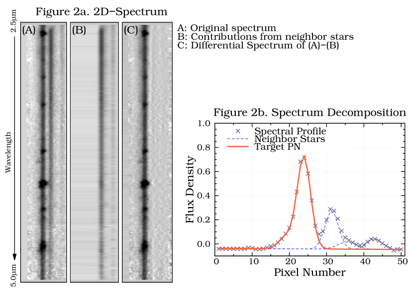
Figure 2: Schematic view of the spectral decomposition procedure. (Left) Panels A, B, and C represent an original two-dimensional spectrum, estimated contributions from the neighboring stars, and an isolated target spectrum. (Right): Spatial profiles of the two-dimensional spectrum (Panel A of Figure 2a). The profiles are decomposed by fitting (see, text). The contributions from neighboring stars are shown by the blue dashed lines. The component of the target is shown by the red solid line.

It was difficult to use a wide aperture for objects which were located in crowded regions. Noble et al. (2013) invented a novel method to extract the spectrum of a certain object in a crowded region by profile fitting. We used a similar method to remove the contribution from neighboring objects. Figure 2 shows a schematic view of the method (hereafter, the spectral decomposition procedure). Panel A of Figure 2a shows an example two-dimensional spectrum of a target in a crowded region. The horizontal and vertical axes correspond to the position and wavelength. The spectrum of the target PN runs through the center of the panel. The spectra of neighboring objects are located to the right side of the PN spectrum. Figure 2b shows the spatial profiles of the spectra (Panel A). The spectra were decomposed by fitting with a combination of Gaussian functions. The red solid line shows the PN profile, and the blue dashed lines show those of the neighboring objects. The fitting was performed for every spectral element. The instrumental spatial profile of a spectrum was not a Gaussian, rather a combination of Gaussian profiles provided the best fit to the profile. Panel B of Figure 2a shows the estimated contribution from the neighboring objects. By subtracting Panel B from Panel A, the two-dimensional spectrum of the target PN was extracted (Panel C). Finally, the one-dimensional spectrum of the target PN was obtained from Panel C with a wide aperture, as mentioned above. The uncertainty in the contamination-corrected spectrum was estimated by taking into account errors in the spectral decomposition procedure. The targets which are in crowded regions are denoted in the ninth column of Table 1.

3.2.1 Subtraction of Contamination

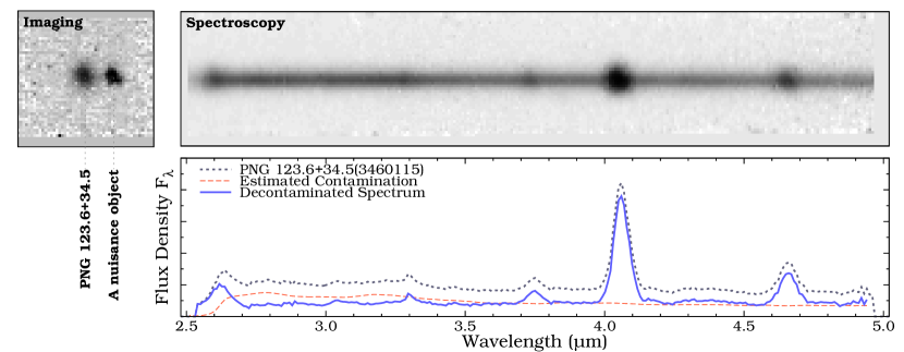
Figure 3: Schematic view of the decontamination procedure. The upper left panel shows the locations of a PN and an overlapping star, while the upper right panel shows the obtained spectrum with contamination from the overlapping star. The contaminated spectrum is shown by the gray dotted line in the bottom panel. The red dashed line shows the estimated contamination from the overlapping star. The decontaminated spectrum of the PN is shown by the blue solid line.

For some observations, the targets were found to be aligned with neighboring objects, along the direction of dispersion. In such cases, the spectra of these objects fully overlapped with each other. This made retrieval of the target profile spectrum, by profile fitting alone, impossible (see the upper panels in Figure 3). To remove the contamination from the overlapping objects, we developed a method to estimate the amount of the contamination (hereafter, the decontamination procedure). The method basically follows the procedure used in Sakon et al. (2008). At first, a one-dimensional spectrum was extracted with a wide aperture. We assumed that overlapping objects were stars and their spectra did not show any particular spectral features in the spectral range in question. Their 2.5–5.0$\,\mu$m spectra ($\tilde{f}_{\nu}$) were estimated from the 2MASS, AKARI, and WISE photometric data by fitting with a blackbody function. The calibration of the overlapping objects required correction since the overlapping object was shifted along the direction of dispersion. The amount of contamination $f^{c}_{\nu}(\lambda)$ was converted from $\tilde{f}_{\nu}$ using the distance between the target and the overlapping objects in the direction of the dispersion, $d$, in units of pixel and the spectral response function of the IRC, $R(\lambda)$, in units of ${\rm ADU}\,{\rm mJy^{-1}}$. We defined $\delta$ as the pixel scale of the spectrum in units of $\mu$m$\,{\rm pixel}^{-1}$. The amount of the contamination was estimated by

$$f^{c}_{\nu}(\lambda)=\frac{\tilde{f}_{\nu}(\lambda{-}\delta d)R(\lambda{-}\delta d)}{R(\lambda)}.$$ (1)

We defined $f^{\rm obs}_{\nu}$ as the obtained spectrum, including the contamination. The decontaminated spectrum was defined by $f^{\rm obj}_{\nu}=f^{\rm obs}_{\nu}-f^{c}_{\nu}$. A schematic view of the method is given in Figure 3. The upper left panel shows the location of the target (PN G123.6+34.5) and overlapping object. The direction of dispersion is horizontal. The spectrum with the contamination is shown in the upper right panel. The contaminated one-dimensional spectrum is shown by the gray dotted line in the bottom panel. The estimated contamination and decontaminated spectra are shown by the red dashed and blue solid lines. We assume that the spectrum of the overlapping star does not have any significant features and that the decontamination procedure does not affect the estimate of emission feature intensities (although continuum flux could be somewhat affected). The targets with overlapping objects are flagged as contaminated objects in the tenth column of Table 1.

4 Results

4.1 Near-Infrared Spectroscopy of Planetary Nebulae Spectral Atlas

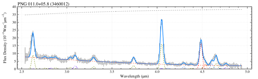
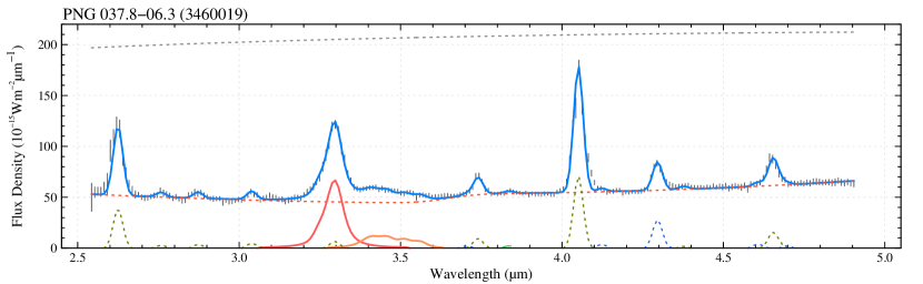
Figure 7: Cont.—

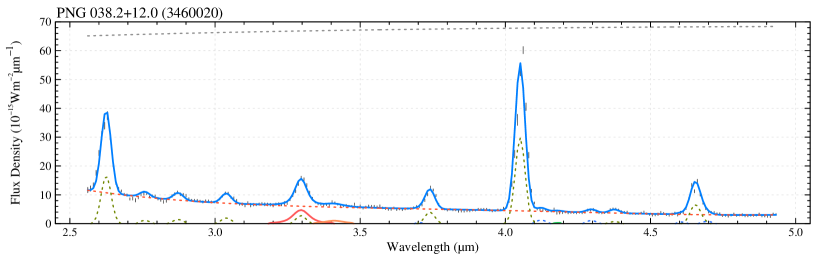
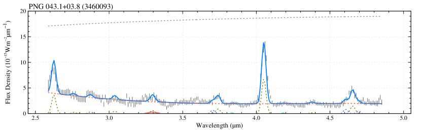
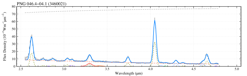
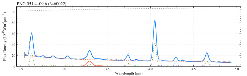
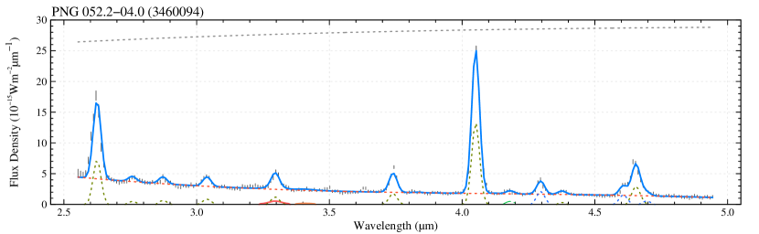
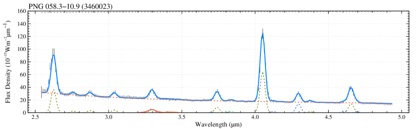
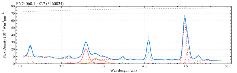
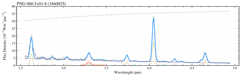
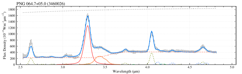
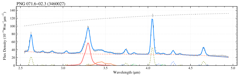
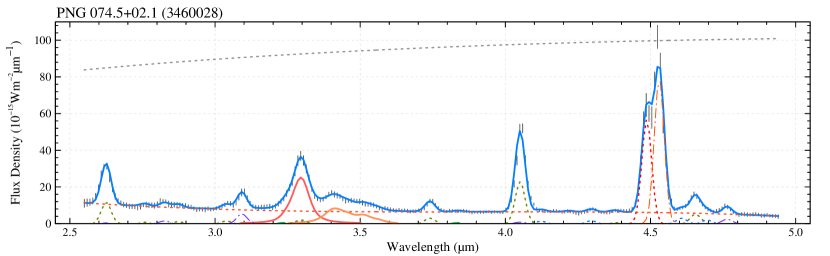
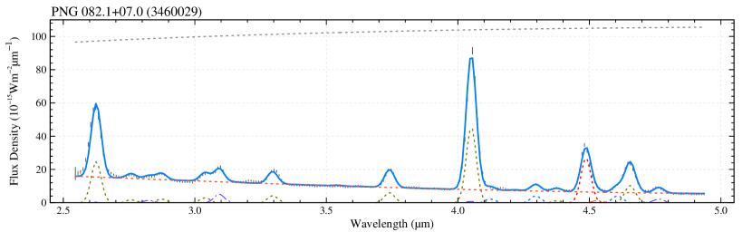
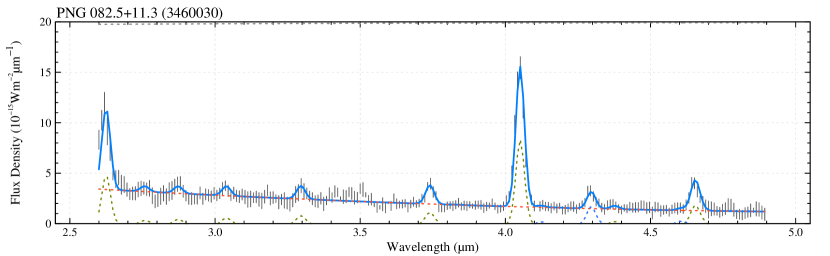
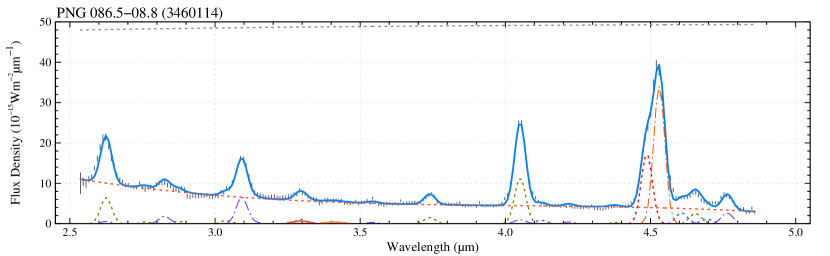
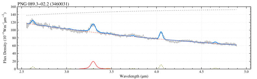
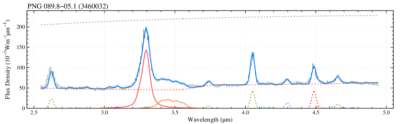
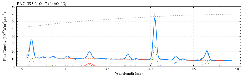
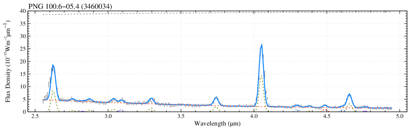
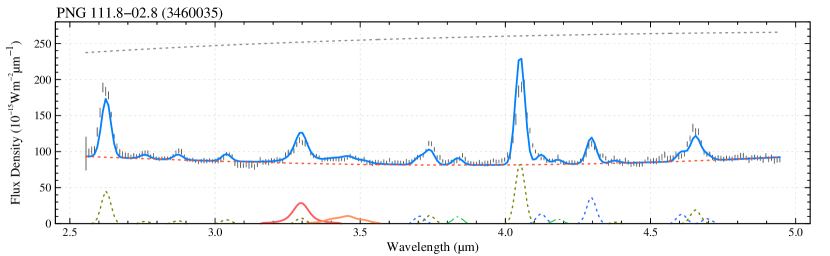
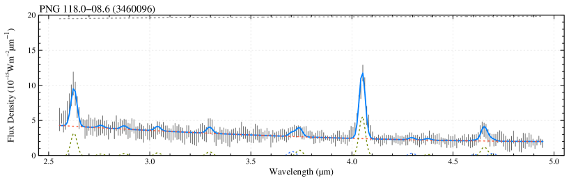
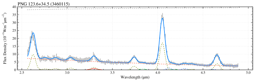
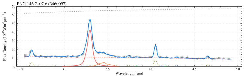
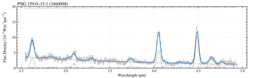
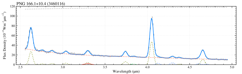
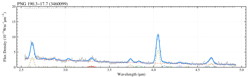
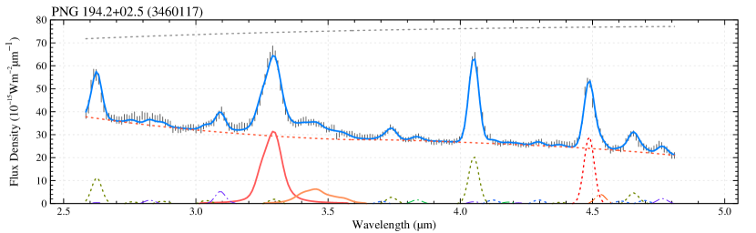
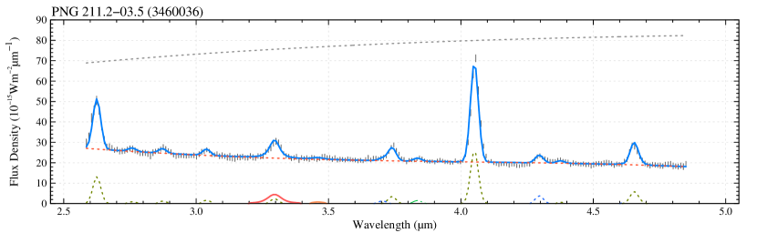
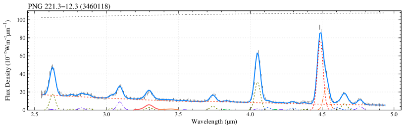
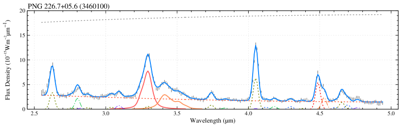
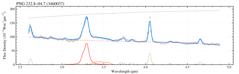
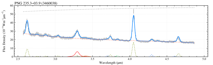
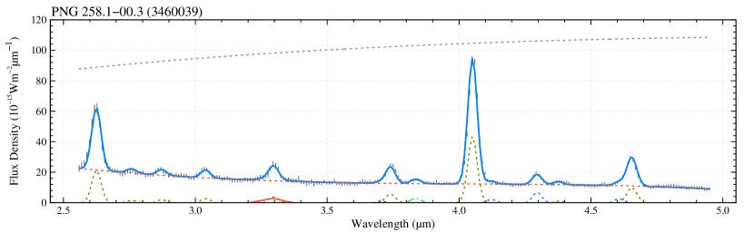
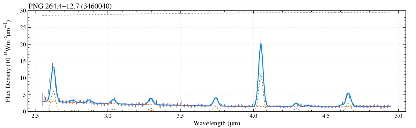
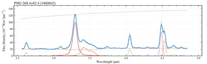
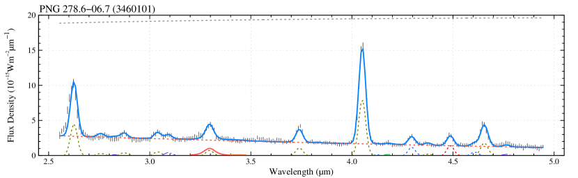
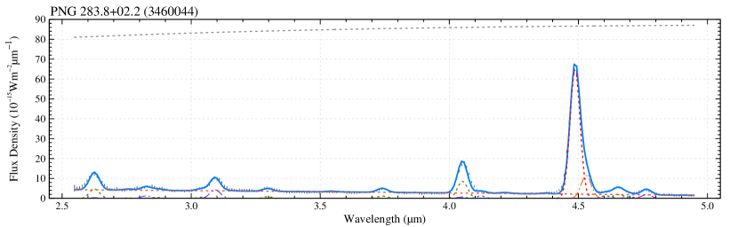
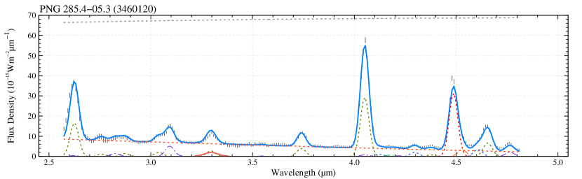
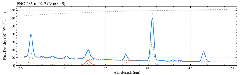
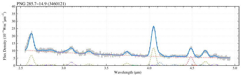
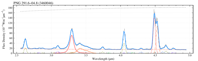
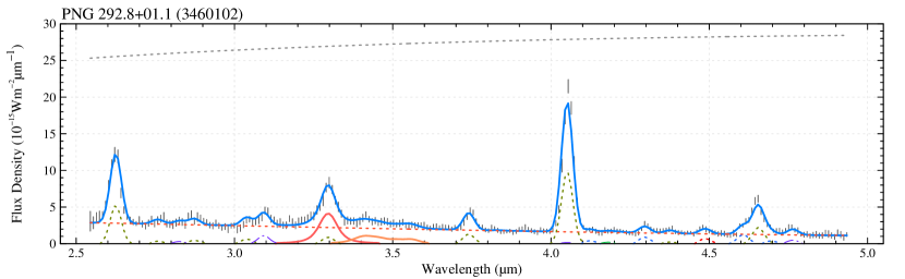
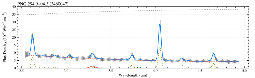
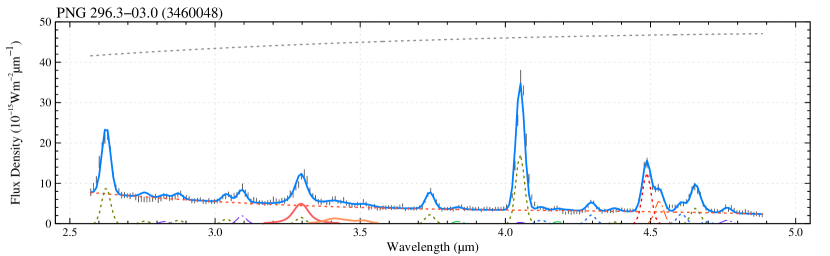
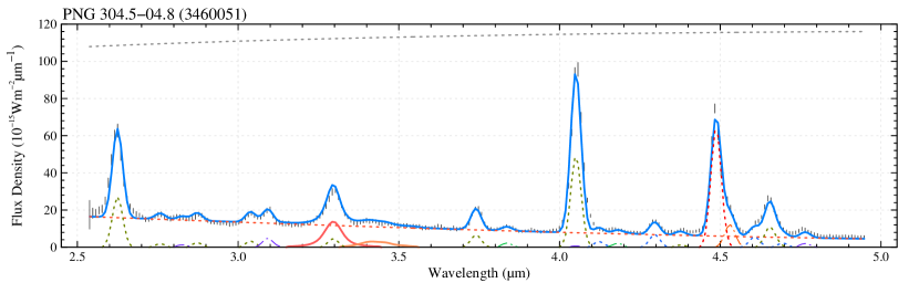
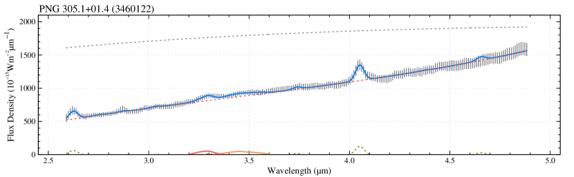
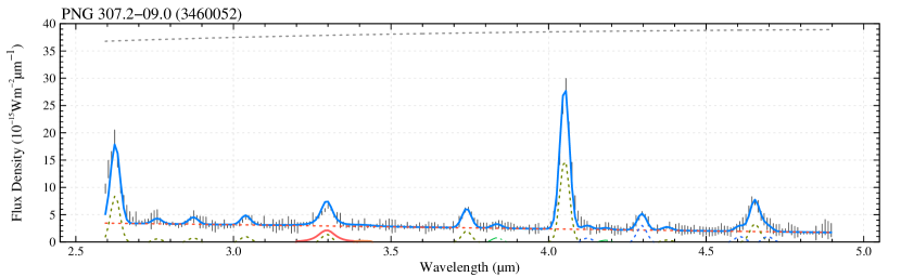
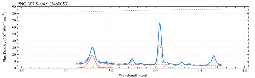
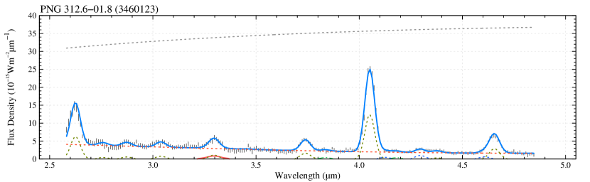
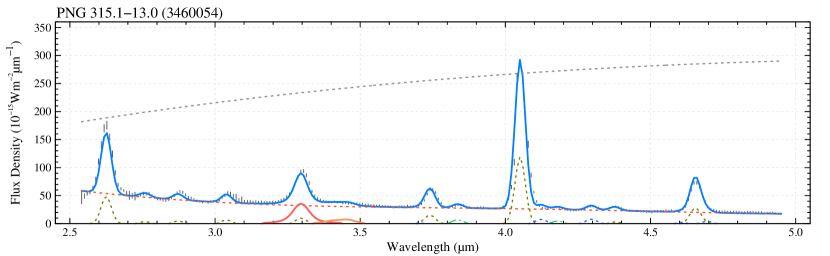
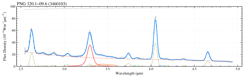
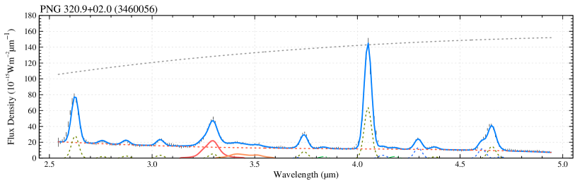
Figure 7: Cont.—

Figure 7: Cont.—

Figure 7: Cont.—

Figure 7: Cont.—

Figure 7: Cont.—

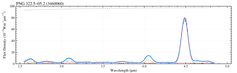
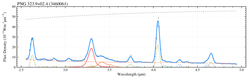
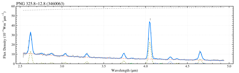
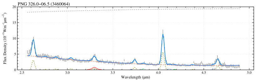
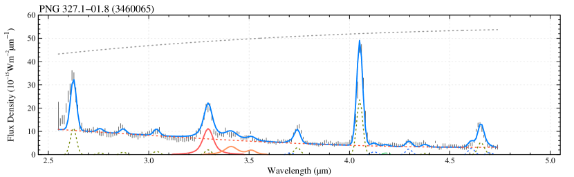
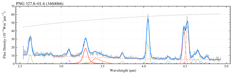
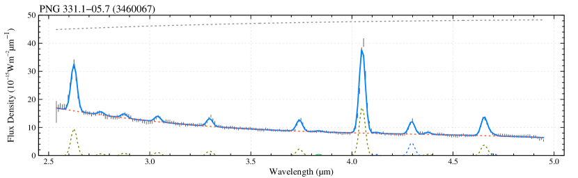
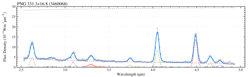
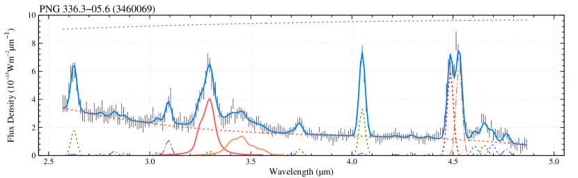
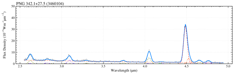
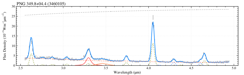
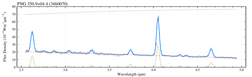
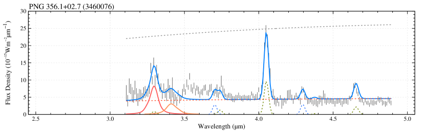
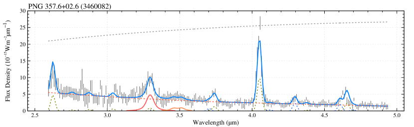
Figure 7: Cont.—

Details of the observations are summarized in Table 1, which includes the PNG ID, the observation ID, the location, the number of exposures, the total integration time, the spectral PSF size, and the flags to denote data quality. The PNSPC catalog contains extracted one-dimensional spectra shown in Figure 7 (plots for all the sources are available in the electric edition). Most of the spectra cover $2.5$–$5.0\,\mu$m. Some spectra were affected by scattered light inside the instrument or column-pull-down effects of the detector, which were not correctable at present. The part of the spectrum severely affected by such issues has been excluded from the catalog.

Two representative spectra in the PNSPC catalog are shown in Figure 4. The top panel is the spectrum of PNG 064.7$+$05.0, and the bottom panel is that of PNG 074.5$+$02.1. The spectra showed several emission features: H I and He II recombination lines, the PAH feature at $3.3\,\mu$m, and the aliphatic feature complex in $3.4$–$3.5\,\mu$m. Some spectra also showed He II recombination lines and [Mg IV] at ${\rm 4.49\,\mu m}$ and [Ar VI] at ${\rm 4.53\,\mu m}$ fine-structure lines, indicating that the excitation of the object was high. Some objects showed molecular hydrogen lines, but they were weak and not frequently detected. No prominent absorption features were detected in any of the objects.

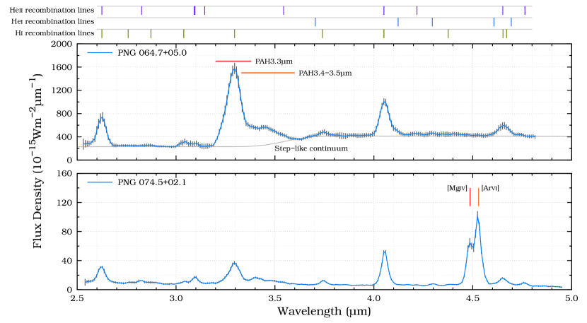
Figure 4: Representative spectra in the PNSPC catalog. The top and bottom panels show the spectra of PNG 064.7$+$05.0 and PNG 074.5$+$02.1 by the blue solid lines with errors. Series of recombination lines (H I, He I, and He II) are indicated by the vertical lines. The both spectra show the PAH feature in 3.3$\,\mu$m and the aliphatic feature complex in 3.4–3.5$\,\mu$m. The spectrum of PNG 074.5$+$02.1 shows fine-structure lines of [Mg IV] at 4.487$\,\mu$m and [Ar VI] at 4.530$\,\mu$m. Step-like continuum emission is seen in the spectra of PNG 064.7$+$05.0 (see Section 4.3).

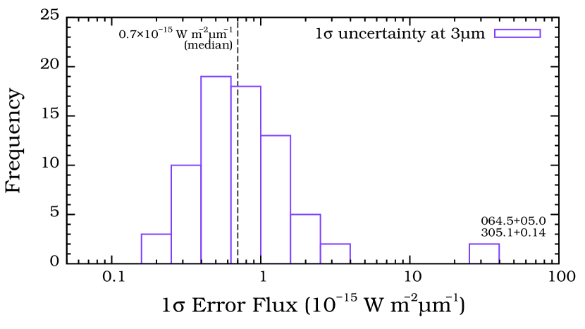
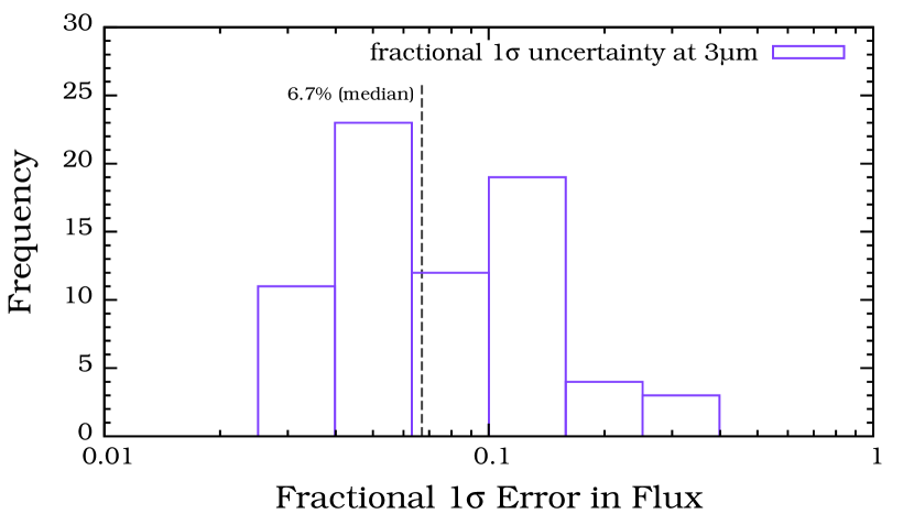
Figure 5: Histograms of the uncertainty in continuum emission at $3.0\,\mu$m. The top panel shows the histogram of absolute 1$\sigma$ errors. The gray dashed line indicates the median of the uncertainty ($0.7{\times}10^{-15}\,{\rm W\,m^{-2}\,\mu m^{-1}}$). The data around 30$\mathit{\times}10^{-15}\,{\rm W\,m^{-2}\,\mu m^{-1}}$ are very bright sources of PNG 064,7${+}$0.5 and 305.1${+}$01.4, for which the spectra were entirely saturated in the long exposure images. The bottom panel shows the histogram of fractional 1$\sigma$ errors. The median value (${\sim}$6.7$\%$) is shown by the gray dashed line.

The top panel of Figure 5 shows a histogram of the uncertainty in continuum emission at $3.0\,\mu$m. The gray dashed line indicates the median of the uncertainty, which is about $0.7{\times}10^{-15}\,{\rm W\,m^{-2}\,\mu m^{-1}}$ or $2\,$mJy. When the object is brighter than $2$–$5{\times}10^{-13}\,{\rm W\,m^{-2}\,\mu m^{-1}}$, the pixels become saturated in the long exposure image. For moderately bright objects, pixels around emission lines were saturated. The spectra of extremely bright objects were completely saturated in the long exposure images. The signal-to-noise ratio of the spectrum depends on the fraction of saturated pixels. PNG 064.7${+}$05.0 and 305.1${+}$01.4 are extremely bright, with their spectrum completely saturated in the long exposure images. Figure 5 (top) indicates that their uncertainties at $3.0\,\mu$m are about 50 times worse than the others. The fractional uncertainty at $3.0\,\mu$m is shown in the bottom panel of Figure 5. The median of the fractional uncertainty is about 6.4%, indicated by the vertical dashed line. This means that, for half of the PNSPC samples, the continuum emission at $3.0\,\mu$m was detected with a signal-to-noise ratio larger than about 15.

The full width half maximum (FWHM) of the spectral PSF of the IRC, equivalent to the FWHM of an unresolved emission line, is about $0.035\,\mu$m. Thus, the spectral resolution is about $\lambda/\Delta\lambda\sim 100$. When the object is extended for the IRC, the spectral resolution is degraded. The FWHM of the spectral PSF, estimated from spectral fitting (see Section 4.3), is listed in the seventh column of Table 1. PN G322.5${-}$05.2 is the most extended object in the PNSPC catalog and its spectral resolution was estimated to be about $\lambda/\Delta\lambda\sim 40$ at 4$\,\mu$m.

4.2 Extinction

Foreground extinction towards the objects was estimated based on an intensity ratio of H$\beta$ to Brackett-$\alpha$ (Br$\alpha$). The intensities of H$\beta$ were obtained from literature (Acker et al., 1992, and references therein). We measured the intensities of Br$\alpha$ from the AKARI spectra by fitting with a Gaussian function. We defined $I_{\rm H\beta}$ and $I_{\rm Br\alpha}$ as the intensities of H$\beta$ and Br$\alpha$. The observed intensity ratio follows the relation:

$$\frac{I_{\rm H\beta}^{\rm obs}}{I_{\rm Br\alpha}^{\rm obs}}=\frac{I_{\rm H\beta}^{0}{\rm e}^{-\tau_{\rm H\beta}}}{I_{\rm Br\alpha}^{0}{\rm e}^{-\tau_{\rm Br\alpha}}},$$ (2)

where $I^{\rm obs}_{X}$ and $I^{0}_{X}$ are the observed and intrinsic intensities of the line $X$, and $\tau_{X}$ is the extinction of the line $X$. We assumed that the nebula was totally opaque for Lyman photons (Case B in Baker & Menzel (1938)). Then, the intrinsic intensity ratio $\left({I_{\rm H\beta}^{0}}/{I_{\rm Br\alpha}^{0}}\right)$ was assumed to be ${\sim}12.853$, given by the Case B line ratio calculated for the electron density of $10^{4}\,{\rm cm^{-3}}$ and the electron temperature of $10^{4}\,$K from Storey & Hummer (1995). We adopted the extinction curve given by Mathis (1990) and the extinction at the $V$-band was derived as

$${\rm A}_{V}({\rm H\beta})=2.39-0.95\ln\left(\frac{I_{\rm H\beta}^{\rm obs}}{I_{\rm Br\alpha}^{\rm obs}}\right).$$ (3)

The coefficients in Equation (3) depends on the assumed electron temperature and density. When the assumed electron temperature increases to $2{\times}10^{4}\,$K, ${\rm A}_{V}$ will increase by about 0.3. The effect of the electron density on ${\rm A}_{V}$ is much smaller than 0.3 for the range from $10^{2}$ to $10^{6}\,{\rm cm^{-3}}$. The systematic uncertainty in ${\rm A}_{V}$, chiefly attributable to the electron temperature uncertainty, was estimated to be less than $0.3\,$mag. The estimated ${\rm A}_{V}({\rm H\beta})$ is listed in the fourth colunm of Table AKARI/IRC Near-Infrared Spectral Atlas of Galactic Planetary Nebulae.

4.3 Spectral Fitting

The intensities of the spectral features were measured by spectral fitting. The fitted function was assumed to be a linear combination of the spectral features as

$$F_{\lambda}(\lambda)=\Bigl{[}f_{\lambda}^{\rm cont}(\lambda)+f_{\lambda}^{\rm line}(\lambda)+f_{\lambda}^{\rm dust}(\lambda)\Bigr{]}{\rm e}^{-\tau(\lambda)},$$ (4)

where $f_{\lambda}^{\rm cont}$, $f_{\lambda}^{\rm line}$, and $f_{\lambda}^{\rm dust}$ were the components of continuum, emission lines, and dust features, and $\tau(\lambda)$ was the optical depth at $\lambda$. The functional shape of $\tau(\lambda)$ was given by a cubic spline function that interpolated the extinction curve of Mathis (1990) at every data point of the IRC spectrum. The amount of the extinction at the $V$-band, ${\rm A}_{V}=\tau(V)$, was included as a fitting parameter.

The continuum emission, $f_{\lambda}^{\rm cont}$, was given by a polynomial function, $f_{\lambda}^{\rm cont}=\sum_{l=0}^{N}c_{l}\lambda^{l}$, where $c_{l}$’s were the fitting parameters. The order $N$ was defined for each object, usually $N=2$ or $3$. This was sufficient to represent the contributions from free-free and hot thermal dust emission. Some PNe showed a sudden increase in the continuum emission around $\lambda\sim 3.6\,\mu$m, for instance, PN G064.7${+}$05.0 in Figure 4. The existence of this emission was mentioned in Boulanger et al. (2011), but the carrier of this emission has not been identified. It was difficult to fit this profile with such a low-order polynomial function. Thus, for those objects with such an increase, we added a step-like function in the components of the continuum emission as

$$f_{\lambda}^{\rm cont}(\lambda)=\sum_{l=0}^{N}c_{l}\lambda^{l}+c\left[~{}\frac{1}{2}+\frac{1}{2}{\rm erf}\left(\frac{\lambda-3.65{\,\rm\mu m}}{\Delta_{\rm step}}\right)\,\right],$$ (5)

where $c$ was the fitting parameter, ${\rm erf}(x)$ was the error function, and $\Delta_{\rm step}$ was the width of the step function, which was tentatively fixed at 0.135$\,\mu$m. This component strongly appears in PNG 037.8${-}$06.3, 064.7${+}$050, 089.8${-}$05.1, and 268.4${+}$02.4.

The emission line profile was approximated by a Gaussian function. The line emission component, $f_{\lambda}^{\rm line}$, was approximated by a combination of Gaussian functions:

$$f_{\lambda}^{\rm line}(\lambda)=\sum_{m}\frac{c_{m}}{\sqrt{2\pi}\sigma}\exp\left[\,-\frac{(\lambda-\lambda_{m0})^{2}}{2\sigma^{2}}\,\,\right],$$ (6)

where $\lambda_{m0}$ was the central wavelengths of the $m$-th emission line and $c_{m}$’s were the parameters to indicate the strength of the lines. The central wavelengths were fixed in the fitting. The line width of the Br$\alpha$ line was measured by fitting with a Gaussian function prior to the fitting and the line widths of other emission lines were assumed to be the same as Br$\alpha$. The lines included in the fitting are listed in Table 3. The assignment and central wavelength are shown in the first and second column. In the fitting, we did not include the lines which were apparently not detected. Some of the H I and He II recombination lines appear at the same wavelength and it was impossible to isolate them. Thus, the relative intensities of the H I and He II recombination lines were fixed, assuming the Case B condition. The relative intensity was adopted from Storey & Hummer (1995) for the electron temperature and the electron density of $10^{4}\,$K and $10^{4}\,{\rm cm^{-2}}$. The variations in the relative intensity with the electron temperature and density were almost negligible compared to the uncertainty in the observed spectra.

Table 3: List of Line Features

Name	$\lambda_{0}$ ($\mu$m)
Brakett-$\alpha^{\dagger}$	4.051
Brakett-$\beta^{\dagger}$	2.625
Pfund-$\beta^{\dagger}$	4.653
Pfund-$\gamma^{\dagger}$	3.740
Pfund-$\delta^{\dagger}$	3.296
Pfund-$\epsilon^{\dagger}$	3.039
Pfund-$\zeta^{\dagger}$	2.873
Pfund-$\eta^{\dagger}$	2.758
Humpleys-$\epsilon^{\dagger}$	4.671
Humpleys-$\zeta^{\dagger}$	4.376
He I(3Po-3D)	3.704
He I(1Po-1D)	4.123
He I(3S-3Po)	4.296
He I(1Po-1S)	4.607
He I(3Po-3S)	4.695

Name	$\lambda_{0}$ ($\mu$m)
He II(7-6)‡	3.092
He II(9-7)‡	2.826
He II(8-7)‡	4.764
He II(12-8)‡	2.625
He II(11-8)‡	3.096
He II(10-8)‡	4.051
He II(14-9)‡	3.145
He II(13-9)‡	3.544
He II(12-9)‡	4.218
He II(14-10)‡	4.652
H2(1-0)	2.802
H2(1-0)	3.003
H2(1-0)	3.234
H2(0-0)	3.836
H2(0-0)	4.181
$[$Mg IV$]$	4.487
$[$Ar VI$]$	4.530

The intrinsic spectral profiles of the PAH emission and the aliphatic feature complex were assumed to be given by a combination of Lorentzian functions which need to be convoluted with the resolution given by the instrument. Thus, their spectral profiles were approximated by the Lorentzian function convoluted with the spectral PSF of the IRC, which was approximated by a Gaussian. The component from dust emission, $f_{\lambda}^{\rm dust}$, was defined by

$$f_{\lambda}^{\rm dust}(\lambda)=\sum_{n}\frac{c_{n}}{\pi\sqrt{2\pi}\sigma}\int{\rm d}\lambda^{\prime}{\rm e}^{-\frac{(\lambda-\lambda^{\prime})^{2}}{2\sigma^{2}}}\frac{\Delta_{n}}{\Delta_{n}^{2}+(\lambda^{\prime}-\lambda_{n0})^{2}},$$ (7)

where $\Delta_{n}$ and $\lambda_{n0}$ were the width and peak wavelength of the $n$-th dust emission and $c_{n}$’s were the fitting parameters. The adopted values of $\Delta_{n}$’s and $\lambda_{n0}$’s were listed in Table 4. The PAH feature at 3.3$\,\mu$m was mainly composed of the 3.30$\,\mu$m feature, but the 3.25$\,\mu$m feature was added to account for a slight change in the spectral profile of the 3.3$\,\mu$m feature. For instance the 3.3$\,\mu$m feature of PNG 320.9${+}$02.0 show an extended blue component, which cannot be well-fitted without the 3.25$\,\mu$m component. Mori et al. (2012) used a combination of four Lorentzian functions to describe the 3.4–3.5$\,\mu$m feature complex (C−H_al) in spectra obtained with the IRC. We used a combination of the four components to describe the C−H_al feature. The central wavelengths and widths were adopted from Mori et al. (2012).

Table 4: List of Dust Features

Name	$\lambda_{0}$ ($\mu$m)	$\Delta$ ($\mu$m)
PAH 3.25†	3.248	0.005
PAH 3.30†	3.296	0.021
C−Hal 3.41‡	3.410	0.030
C−Hal 3.46‡	3.460	0.013
C−Hal 3.51‡	3.512	0.013
C−Hal 3.56‡	3.560	0.013

Define $F_{\lambda}^{\rm obj}(\lambda)$ and $\sigma_{\lambda}(\lambda)$ as the observed flux and its uncertainty at $\lambda$. We assumed that the residual $\Delta_{\lambda}(\lambda)=F_{\lambda}^{\rm obj}(\lambda)-F_{\lambda}(\lambda)$ followed a normal distribution with the variance of $\sigma^{2}_{\lambda}(\lambda)$. The likelihood function was defined as

$$\mathcal{L}\propto\prod_{i}\exp\left[-\frac{1}{2}\left(\frac{\Delta_{\lambda}(\lambda_{i})}{\sigma_{\lambda}(\lambda_{i})}\right)^{2}\right],$$ (8)

where $\lambda_{i}$ was the wavelength of the $i$-th spectral element. The fitting parameters could be defined by maximizing Equation (8). However, it was difficult to accurately derive the amount of the extinction, ${\rm A}_{V}$, only from the near-infrared spectrum (see, Appendix A). To make the fitting stable, we used the extinction estimated in Section 4.2 to provide a prior distribution of the extinction

$$P({\rm A}_{V})\propto\exp\left[-\frac{1}{2}\left(\frac{{\rm A}_{V}{-}{\rm A}_{V}({\rm H\beta})}{\sigma^{\prime\prime}}\right)^{2}\right],$$ (9)

where ${\rm A}_{V}({\rm H\beta})$ was the extinction estimated from the H$\beta$ to Br$\alpha$ intensity ratio and $\sigma^{\prime\prime}$ was tentatively fixed at $0.3\,$mag, estimated from the systematic error. The fitting parameters were derived by maximizing the product of Equations (8) and (9) with the constraints that the parameters of ${\rm A}_{V}$, $c$, $c_{m}$ and $c_{n}$ should be non-negative. The uncertainties of the fitting parameters were estimated based on a Monte Carlo simulation: The spectrum of the target, $\tilde{F}(\lambda)$ was simulated assuming a normal distribution of flux with a mean of $F^{\rm obj}_{\lambda}(\lambda)$ and a variance of $\sigma_{\lambda}(\lambda)$. The fitting parameters were derived for $\tilde{F}(\lambda)$. This procedure was repeated 1 000 times and the probability distributions of the fitting parameters were obtained. The confidence interval of the fitting parameters was defined to account for 68% of the trials.

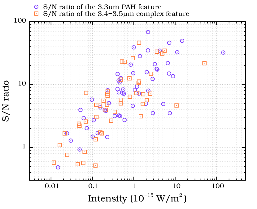
Figure 6: The signal-to-noise ratio (${\rm S/N}$) is plotted against the intensity of the emission features, indicating a typical detection limit of emission features. The blue circles represent the ${\rm S/N}$ ratio of the 3.3$\,\mu$m PAH feature, while the red squares show that of the 3.4–3.5$\,\mu$m aliphatic feature complex.

The extinction obtained by the fitting (${\rm A}_{V}(\rm fit.)$) is listed in the fifth column of Table AKARI/IRC Near-Infrared Spectral Atlas of Galactic Planetary Nebulae. Table 5 lists the extinction-corrected intensities of Br$\alpha$ at $4.05\,\mu$m, He I at $4.30\,\mu$m, He II at $3.09\,\mu$m, the PAH feature at $3.3\,\mu$m, the aliphatic feature complex in $3.4$–$3.5\,\mu$m, [Mg IV] at $4.49\,\mu$m, and [Ar VI] at $4.53\,\mu$m. These emission features were strong and widely detected among the PNSPC samples. Other line features were weak or not detected in the majority of the targets and thus were not included in the table. The equivalent widths of those are listed in Table 6. Note that [Mg IV] and [Ar VI] are so close that their spectral profiles are in part overlapping. Their uncertainties are relatively large compared to other lines, because the effect of overlapping was taken into account. Figure 6 shows the signal-to-noise ratio against the intensity of the $3.3\,\mu$m PAH feature and the 3.4–3.5$\,\mu$m aliphatic feature complex by the blue circles and the red squares. Figure 6 indicates that the emission feature stronger than ${\sim}2{\times}10^{-16}\,{\rm W\,m^{-2}}$ was detected with a 3$\sigma$-confidence level.

Table 5: Extinction Corrected Line Intensity

PN G	Bracket-$\alpha$	He II$(3.09{\rm\mu m})$	He I$(4.30{\rm\mu m})$	PAH$(3.3{\rm\mu m})$	C−Hal$(3.4$-$3.5{\rm\mu m})$	[Mg IV]$(4.49{\rm\mu m})$	[Ar VI]$(4.53{\rm\mu m})$
	$10^{-15}\,{\rm W\,m^{-2}}$	$10^{-15}\,{\rm W\,m^{-2}}$	$10^{-15}\,{\rm W\,m^{-2}}$	$10^{-15}\,{\rm W\,m^{-2}}$	$10^{-15}\,{\rm W\,m^{-2}}$	$10^{-15}\,{\rm W\,m^{-2}}$	$10^{-15}\,{\rm W\,m^{-2}}$
000.3${+}$12.2	$\phantom{0}\phantom{0}\phantom{0}2.74_{{-}0.04}^{{+}0.05}$	$\cdots$	$\phantom{0}\phantom{0}\phantom{0}0.14_{{-}0.03}^{{+}0.03}$	${<}0.11$	$\cdots$	$\cdots$	$\cdots$
002.0${-}$13.4	$\phantom{0}\phantom{0}\phantom{0}2.05_{{-}0.03}^{{+}0.04}$	$\cdots$	$\phantom{0}\phantom{0}\phantom{0}0.31_{{-}0.02}^{{+}0.03}$	$\phantom{0}\phantom{0}\phantom{0}0.25_{{-}0.05}^{{+}0.05}$	${<}0.10$	$\cdots$	$\cdots$
003.1${+}$02.9	$\phantom{0}\phantom{0}\phantom{0}3.16_{{-}0.04}^{{+}0.04}$	${<}0.53$	$\phantom{0}\phantom{0}\phantom{0}0.43_{{-}0.04}^{{+}0.03}$	$\phantom{0}\phantom{0}\phantom{0}0.94_{{-}0.16}^{{+}0.25}$	$\phantom{0}\phantom{0}\phantom{0}0.49_{{-}0.08}^{{+}0.09}$	$\phantom{0}\phantom{0}\phantom{0}0.35_{{-}0.04}^{{+}0.05}$	$\cdots$
011.0${+}$05.8	$\phantom{0}\phantom{0}\phantom{0}1.09_{{-}0.04}^{{+}0.03}$	$\phantom{0}\phantom{0}\phantom{0}0.13_{{-}0.03}^{{+}0.03}$	${<}0.13$	$\cdots$	$\cdots$	$\phantom{0}\phantom{0}\phantom{0}1.11_{{-}0.08}^{{+}0.05}$	$\phantom{0}\phantom{0}\phantom{0}0.20_{{-}0.05}^{{+}0.04}$
027.6${-}$09.6	$\phantom{0}\phantom{0}\phantom{0}1.12_{{-}0.02}^{{+}0.04}$	$\cdots$	$\phantom{0}\phantom{0}\phantom{0}0.10_{{-}0.01}^{{+}0.01}$	$\cdots$	$\cdots$	$\cdots$	$\cdots$
037.8${-}$06.3	$\phantom{0}\phantom{0}\phantom{0}4.61_{{-}0.10}^{{+}0.24}$	$\cdots$	$\phantom{0}\phantom{0}\phantom{0}1.80_{{-}0.09}^{{+}0.13}$	$\phantom{0}\phantom{0}\phantom{0}6.64_{{-}0.21}^{{+}0.40}$	$\phantom{0}\phantom{0}\phantom{0}2.60_{{-}0.14}^{{+}0.21}$	$\cdots$	$\cdots$
038.2${+}$12.0	$\phantom{0}\phantom{0}\phantom{0}2.18_{{-}0.06}^{{+}0.04}$	$\cdots$	${<}0.13$	$\phantom{0}\phantom{0}\phantom{0}0.45_{{-}0.05}^{{+}0.04}$	$\phantom{0}\phantom{0}\phantom{0}0.12_{{-}0.02}^{{+}0.03}$	$\cdots$	$\cdots$
043.1${+}$03.8	$\phantom{0}\phantom{0}\phantom{0}0.45_{{-}0.01}^{{+}0.01}$	$\cdots$	$\cdots$	${<}0.06$	${<}0.01$	$\cdots$	$\cdots$
046.4${-}$04.1	$\phantom{0}\phantom{0}\phantom{0}2.43_{{-}0.01}^{{+}0.02}$	$\phantom{0}\phantom{0}\phantom{0}0.11_{{-}0.02}^{{+}0.02}$	$\phantom{0}\phantom{0}\phantom{0}0.32_{{-}0.01}^{{+}0.02}$	$\phantom{0}\phantom{0}\phantom{0}0.40_{{-}0.05}^{{+}0.04}$	${<}0.16$	$\cdots$	$\cdots$
051.4${+}$09.6	$\phantom{0}\phantom{0}\phantom{0}3.25_{{-}0.02}^{{+}0.06}$	$\cdots$	$\phantom{0}\phantom{0}\phantom{0}0.52_{{-}0.02}^{{+}0.02}$	$\phantom{0}\phantom{0}\phantom{0}0.97_{{-}0.07}^{{+}0.05}$	$\phantom{0}\phantom{0}\phantom{0}0.23_{{-}0.05}^{{+}0.04}$	$\cdots$	$\cdots$

Note. — ^†,‡: relative intensities of these lines are fixed assuming the Case B condition.

Note. — ^†: they belong to the PAH feature at 3.3$\,\mu$m. ^‡: they belong to the aliphatic feature complex in 3.4–3.5$\,\mu$m.

Note. — Table 5 is published in its entirety in the electronic edition of the Astrophysical Journal. A portion is shown here for guidance regarding its form and content.

Table 6: Extinction Corrected Line Equivalent Width

PN G	Bracket-$\alpha$	He II$(3.09{\rm\mu m})$	He I$(4.30{\rm\mu m})$	PAH$(3.3{\rm\mu m})$	C−Hal$(3.4$-$3.5{\rm\mu m})$	[Mg IV]$(4.49{\rm\mu m})$	[Ar VI]$(4.53{\rm\mu m})$
	Å	Å	Å	Å	Å	Å	Å
000.3${+}$12.2	$\phantom{0}2825.6_{{-}38.2}^{{+}47.3}$	$\cdots$	$\phantom{0}\phantom{0}154.5_{{-}32.7}^{{+}35.5}$	${<}130.7$	$\cdots$	$\cdots$	$\cdots$
002.0${-}$13.4	$\phantom{0}2938.4_{{-}39.9}^{{+}64.0}$	$\cdots$	$\phantom{0}\phantom{0}481.9_{{-}27.1}^{{+}42.1}$	$\phantom{0}\phantom{0}435.3_{{-}84.6}^{{+}86.8}$	${<}181.4$	$\cdots$	$\cdots$
003.1${+}$02.9	$\phantom{0}2105.7_{{-}25.5}^{{+}26.5}$	${<}236.7$	$\phantom{0}\phantom{0}343.7_{{-}30.2}^{{+}25.6}$	$\phantom{0}\phantom{0}665.7_{{-}113.7}^{{+}176.0}$	$\phantom{0}\phantom{0}365.1_{{-}59.5}^{{+}68.0}$	$\phantom{0}\phantom{0}324.3_{{-}42.0}^{{+}51.4}$	$\cdots$
011.0${+}$05.8	$\phantom{0}2005.1_{{-}68.8}^{{+}61.4}$	$\phantom{0}\phantom{0}144.8_{{-}34.2}^{{+}32.1}$	${<}266.9$	$\cdots$	$\cdots$	$\phantom{0}2605.4_{{-}179.7}^{{+}127.9}$	$\phantom{0}\phantom{0}486.2_{{-}111.4}^{{+}101.8}$
027.6${-}$09.6	$\phantom{0}3229.6_{{-}44.8}^{{+}128.8}$	$\cdots$	$\phantom{0}\phantom{0}328.8_{{-}27.6}^{{+}35.8}$	$\cdots$	$\cdots$	$\cdots$	$\cdots$
037.8${-}$06.3	$\phantom{0}\phantom{0}482.1_{{-}10.0}^{{+}25.4}$	$\cdots$	$\phantom{0}\phantom{0}182.2_{{-}\phantom{0}8.6}^{{+}13.6}$	$\phantom{0}1342.1_{{-}42.1}^{{+}80.2}$	$\phantom{0}\phantom{0}531.1_{{-}29.1}^{{+}42.6}$	$\cdots$	$\cdots$
038.2${+}$12.0	$\phantom{0}2863.3_{{-}84.4}^{{+}54.5}$	$\cdots$	${<}192.5$	$\phantom{0}\phantom{0}709.0_{{-}75.8}^{{+}55.0}$	$\phantom{0}\phantom{0}204.3_{{-}38.7}^{{+}47.2}$	$\cdots$	$\cdots$
043.1${+}$03.8	$\phantom{0}1316.2_{{-}37.5}^{{+}42.9}$	$\cdots$	$\cdots$	${<}230.0$	$\cdots$	$\cdots$	$\cdots$
046.4${-}$04.1	$\phantom{0}3171.2_{{-}\phantom{0}5.0}^{{+}29.3}$	$\phantom{0}\phantom{0}\phantom{0}99.6_{{-}18.0}^{{+}17.8}$	$\phantom{0}\phantom{0}475.1_{{-}\phantom{0}9.3}^{{+}29.6}$	$\phantom{0}\phantom{0}595.7_{{-}75.1}^{{+}65.3}$	${<}250.8$	$\cdots$	$\cdots$
051.4${+}$09.6	$\phantom{0}1882.4_{{-}13.5}^{{+}36.4}$	$\cdots$	$\phantom{0}\phantom{0}315.8_{{-}12.1}^{{+}15.0}$	$\phantom{0}\phantom{0}740.7_{{-}56.1}^{{+}41.7}$	$\phantom{0}\phantom{0}180.1_{{-}42.6}^{{+}32.7}$	$\cdots$	$\cdots$

Note. — Table 6 is published in its entirety in the electronic edition of the Astrophysical Journal. A portion is shown here for guidance regarding its form and content.

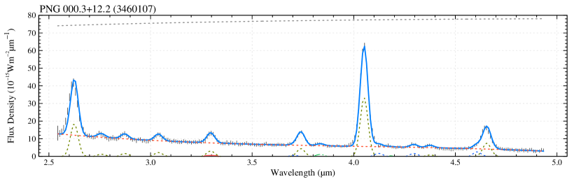
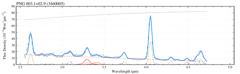
Figure 7: The AKARI/IRC 2.5–5.0$\,\mu$m spectra. Explanations of the lines are shown in the bottom of the figures. Plots for all sources are available in the electronic edition of the journal.

5 Discussion

5.1 Biases in the PNSPC samples

5.1.1 Galactic Coordinates

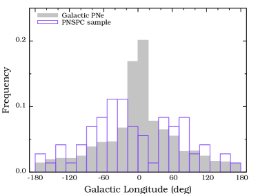
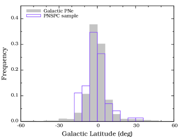
Figure 8: Histograms of PNe in the Galactic coordinates. The left panel shows the histogram of the Galactic longitude, while the right panel shows that of the Galactic latitude. The histograms for the PNSPC objects are shown by the blue boxes. The gray filled boxes represent the distribution of all the Galactic PNe in Acker et al. (1992).

We compare the distribution of the PNSPC samples in the Galactic coordinates with that of the PNe in Acker et al. (1992), which are assumed to represent the distribution of all the PNe in the Milky Way. The histograms of the Galactic longitude and latitude are shown in the left and right panels of Figure 8. The histograms of the PNSPC samples are shown by the blue lines, while the histograms of PNe in Acker et al. (1992) are shown by the gray filled bars. The total number of the PNe in Acker et al. (1992) is 1143. The longitude histogram of the PNSPC samples looks broader than that of the PNe in Acker et al. (1992), while the latitude histogram of the PNSPC samples does not show a large deviation from that of the PNe in Acker et al. (1992). We investigate the differences by Kolmogorov-Smirnov test. The values of $\chi^{2}_{\nu{=}2}$ are about 16 for the longitude and 4 for the latitude. The results suggest that the deviation of the longitude is highly significant and that the PNSPC samples are biased toward PNe in the Galactic disk rather than those in the bulge. Figure 9 shows the position of the PNSPC samples projected onto the Galactic plane. The distances to the objects are taken from literature (Acker, 1978; Pottasch, 1983; Maciel, 1984; Amnuel et al., 1984; Gathier et al., 1986a, b; Sabbadin, 1986; Cahn et al., 1992; Acker et al., 1992, and references therein). Figure 9 shows that most of the PNSPC samples are within $5$ kpc of the Sun, even when accounting for uncertainties in the distance estimate. This also supports that the PNSPC samples mainly consist of PNe in the Galactic disk.

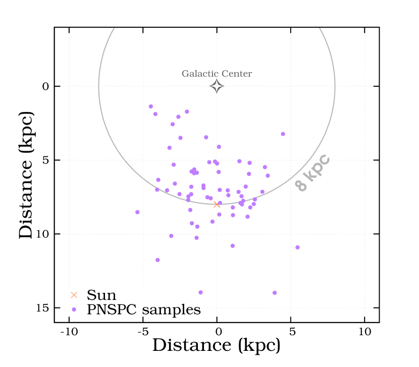
Figure 9: Distribution of the PNSPC samples on the Galactic Plane. The red cross shows the locus of the Sun. The purple circles show the positions of the PNSPC samples.

5.1.2 Effective Temperature and Age

The central star of a PN becomes hot as it evolves. The effective temperature of the PN can be used as an indicator of the age of the PN. The timescale of the evolution depends on the mass of the central star (e.g., Blöcker, 1995; Schönberner, 1983). Although the individual age of the PN is difficult to accurately derive from the effective temperature, the distribution of the effective temperature reflects the bias in the age of the PNSPC samples. The effective temperatures were collected from literature. The temperature and its references are listed in the sixth and seventh columns of Table AKARI/IRC Near-Infrared Spectral Atlas of Galactic Planetary Nebulae. The effective temperature is estimated with several different methods. The effective temperatures estimated based on a model atmosphere should be the most reliable. The temperatures estimated in Mendez et al. (1988) and Harrington & Feibelman (1983) are preferentially used, if available. The typical error for temperatures measured by this method is about 10% (Mendez et al., 1988). Otherwise, the effective temperatures estimated with the Zanstra or the Energy Balance methods are used. The Zanstra temperatures are estimated based on H I, He I, and He II recombination lines. Since the radiation-bounded condition is assumed in the Zanstra method, the Zanstra temperature estimated using the line with the highest ionization potential is most reliable. The Zanstra temperatures are used with the preferential order of He II, He I, and H I. A typical uncertainty in the Zanstra temperature is as large as 10,000 K in the worst case (Phillips, 2003). Preite-Martinez et al. (1991) reported that the typical uncertainty in the temperature with the Energy Balance method is no more than 20%. We assume that a typical uncertainty in these methods is about 20%. Finally, the effective temperature was obtained for $67$ of $72$ objects in the catalog. When multiple references are available, the averaged value is adopted.

Figure 10 shows the distribution of the effective temperature in the PNSPC samples. Phillips (2003) collected the effective temperature of 373 Galactic PNe using the Zanstra method. Their samples were widely collected from literature without any limitation. Thus, we assume that their samples are not biased and that the temperature distribution of Phillips’ samples represents that of the whole Galactic PNe (gray dashed line). The median of the effective temperature for the PNSPC samples is about $50\,000\,{\rm K}$, while that for Phillips’ data is about $80\,000\,{\rm K}$. Figure 10 indicates that the PNSPC samples are biased toward low-temperature or young PNe, possibly due to the target selection bias: the targets are limited by the apparent size (${\sim}3^{\prime\prime}$).

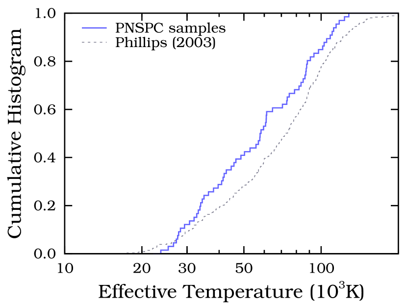
Figure 10: Cumulative histogram of the effective temperature of Galactic PNe. The blue solid line shows the histogram for the PNSPC samples. The gray dashed line represents the temperature distribution of all the Galactic PNe in Phillips (2003).

5.2 Accuracy of the Absolute Intensity

One of the major characteristics of the PNSPC catalog is slit-less spectroscopy in the Np-window, which allows us to collect all of the flux from the target. Since the IRC spectrum totally covers the WISE W1 band, the accuracy of the absolute flux density is evaluated by comparing the PNSPC spectra with the WISE W1 photometry from WISE All-Sky Release Catalog (Cutri et al., 2012). Define $R^{\rm W1}$ as the relative response curve of the WISE W1 band (per photon; Wright et al., 2010). The flux in the W1 band estimated from the IRC spectrum is defined as

$$F^{\rm IRC}_{\nu}({\rm W1})=\frac{\displaystyle\int F^{\rm obj}_{\nu}(\nu)R^{\rm W1}(\nu)\frac{{\rm d}\nu}{\nu}}{\displaystyle\int\left(\frac{\nu_{\rm iso}}{\nu}\right)^{2}R^{\rm W1}(\nu)\frac{{\rm d}\nu}{\nu}},$$ (10)

where $\nu_{\rm iso}$ is the isophotal frequency of the W1 band (3.35$\,\mu$m) and $F^{\rm obj}_{\nu}$ is the observed flux density in units of Jy. Figure 11 shows the estimated flux density in the W1 band against the WISE W1 catalog data. It confirms that the W1 flux density estimated from the IRC spectra, $F^{\rm IRC}_{\nu}({\rm W1})$, is consistent with the WISE W1 data in a wide range from about $0.01$ to $5\,{\rm Jy}$. The histogram of the AKARI to WISE W1 flux ratio is shown in Figure 12. Errors in Figure 12 are calculated by a Monte Carlo simulation with the uncertainty in the flux ratio. The ratios are distributed with the mean of $1.01{\pm}0.01$ and the standard deviation of $0.21{\pm}0.02$. Three PNe (PNG 285.7$-$14.9, 324.8$-$01.1, and 305.1$+$01.4) show significant deviations larger than 50%. For PNG 285.7$-$14.9 and 305.1$+$01.4, their AKARI W1 fluxes are larger than those of WISE. Both objects are apparently extended in WISE W1 images. The deviations may be attributed to the loss of the flux in WISE photometry. Furthermore, PNG 305.1$+$01.4 is the brightest object in the PNSPC sample. The WISE detector starts to saturate in the W1 band at $\sim$0.17$\,{\rm Jy}$ (Wright et al., 2010). This may also cause an error in WISE photometry of PNG 305.1$+$01.4. The AKARI W1 flux of PNG 324.8$-$01.1 is smaller than the WISE W1 flux. PNG 324.8$-$01.1 is located in a crowded region, so that the IRC field of view may not be wide enough to estimate background emission accurately. The loss of the AKARI W1 flux is attributable to the error in the estimation of the background emission. Thus, although the absolute continuum intensity of PNG 324.8$-$01.1 may be erroneous, the intensity of emission features is not affected by the estimation of background emission. The absolute flux of the present catalog is concluded to be accurate within $20$%.

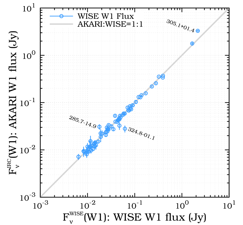
Figure 11: Flux comparison between the AKARI and WISE observations. The vertical axis shows the flux in the WISE W1 filter estimated from the AKARI/IRC spectra, while the horizontal axis shows the flux in the WISE All-Sky Release Catalog (Cutri et al., 2012). When the deviation between the AKARI and WISE W1 fluxes is larger than 50%, the data point is labeled with the PNG ID.

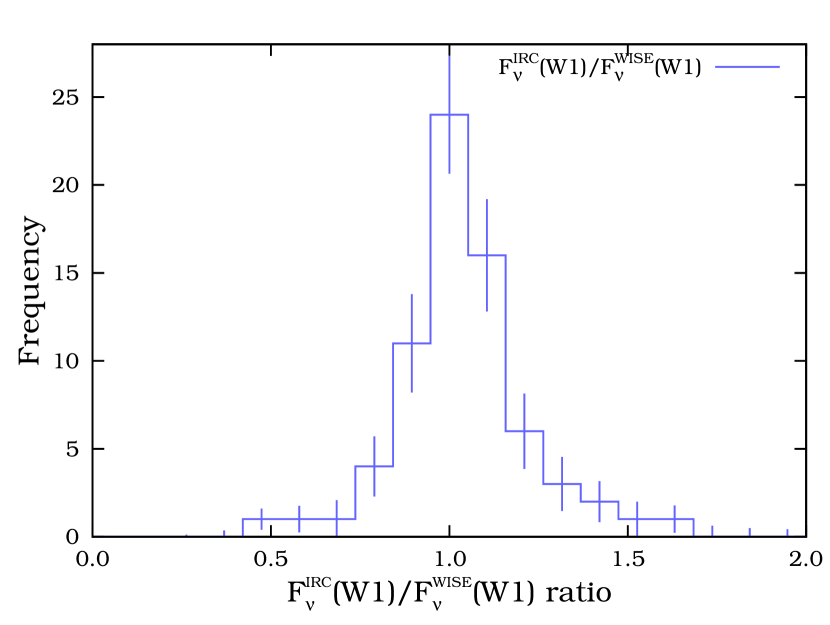
Figure 12: Distribution of the flux ratio: the flux in the WISE W1 filter estimated from the AKARI/IRC spectra to that from the WISE All-Sky Release Catalog.

5.3 Extinction within the Individual Nebula

The PNSPC spectra include Brackett-$\alpha$ (Br$\alpha$), the hydrogen recombination line at 4.05$\,\mu$m, which enables us to estimate the extinction towards the objects using the relative intensity of H$\beta$ to Br$\alpha$ (the intensity of H$\beta$ is from Acker et al. (1992), see Section 4.2). The cumulative histogram of the total extinction towards the PNSPC samples, $A_{V}({\rm H}\beta)$, is shown by the dotted line in Figure 13. The extinction toward the PNSPC samples are less than $6\,$mag. at the $V$-band. About 70% of the PNSPC samples have $A_{\rm V}({\rm H}\beta)<2\,$mag., suggesting that most of the PNSPC samples are not heavily obscured. This is consistent with the Galactic distribution of the PNSPC sample shown in Section 5.1.1.

The extinction values calculated in Section 4.2 include the contribution from their circumstellar envelope, $A_{V,\,{\rm PN}}$, and the interstellar medium to the object, $A_{V,\,{\rm ISM}}$. The contribution from the interstellar medium, $A_{V,\,{\rm ISM}}$, can be estimated using the extinction map based on the Digitized Sky Survey (Dobashi et al., 2005a, b). The extinction map is given in the resolution of $2\arcmin{\times}2\arcmin$. We calculate the averaged extinction values within a $6\arcmin$ radius around the object $A_{V}({\rm DSS})$ and assumed them as $A_{V,\,{\rm ISM}}$. Dobashi et al. (2005a) showed that a systematic error in $A_{V}({\rm DSS})$ is typically less than 0.2 mag for $A_{V}({\rm DSS})<5\,$mag. We estimate the uncertainty in $A_{V,\,{\rm ISM}}$ from the scatter of $A_{V}({\rm DSS})$ within the $6\arcmin$ circle taking into account the systematic error. Note that the extinction $A_{V,\,{\rm ISM}}$ estimated here may have a large uncertainty. The extinction from the circumstellar envelope, defined by $A_{V}({\rm H}\beta)-A_{V}({\rm DSS})$, is shown by the solid line in Figure 13. Some objects show negative extinction values (${\sim}0.5\,$mag.), possibly due to the overestimation of $A_{V,\,{\rm ISM}}$. Figure 14 shows the dependence of $A_{V}({\rm H}\beta)-A_{V}({\rm DSS})$ on the distance towards the PN. We find that PNe with extinction ${>}2\,$mag. frequently appear around 2 kpc. The name of the constellation is added next to those PNe, indicating that most of them are in the regions around Cygnus and Norma as indicated by the orange and green symbols. The extinction $A_{V,\,{\rm ISM}}$ for these PNe may be underestimated or have large local fluctuations, but this affects only about 10% of the PNSPC samples. Except for the objects in the Cygnus and Norma regions, Figure 14 does not show any trend with the distance, suggesting that the $A_{V}({\rm H}\beta)-A_{V}({\rm DSS})$ value is attributable to the extinction internal to the PN. Figure 13 indicates that the median of the circumstellar extinction is about 0.8 mag. and about $40\%$ of the PNe show extinction larger than $1\,$mag. suggesting that the circumstellar envelope of a PN is generally optically thick in the UV. Ohsawa et al. (2012) investigated the spatial distribution of mid-infrared dust emission of PN G095.2${+}$00.7, a young and UV-thick Galactic PN, and suggest that the evolution of a UV-thick circumstellar envelope may have a significant impact on the appearance of the mid-infrared spectrum of the PN. The present results suggest that PNe spectra should be investigated by taking into account the radiation transfer within the nebula, and the gradient in the dust temperature.

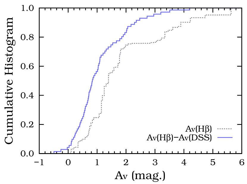
Figure 13: Cumulative histogram of the extinction at the $V$-band. The dotted line shows the histogram of the total extinction towards the PN. The solid line shows the histogram of the extinction without the contribution from the interstellar medium.

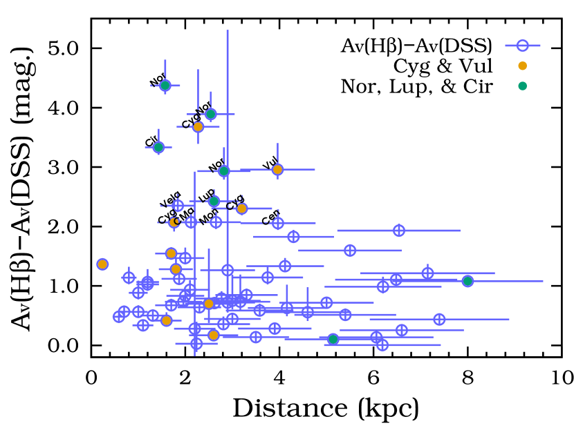
Figure 14: Net extinction at the $V$-band is plotted against a distance towards the PN. Errors in the distance are assumed to be about 20%. The name of the constellation is added next to the symbols for the PN with the net extinction ${>}2.0\,$mag. The PNe in Cygnus and Vulpecula are indicated by the orange filled circles, while the PNe in Norma, Lupus and Circinus are indicated by the green filled circles.

5.4 Equivalent Width of Ionized Gas Emission Lines

The spectra in the PNSPC catalog contain several emission lines, including hydrogen and helium recombination lines and fine-structure lines of [Mg IV] at 4.49$\,\mu$m and [Ar VI] at 4.53$\,\mu$m. These emission lines should reflect the characteristics of the radiation field of the circumstellar envelope. Figure 15 shows the equivalent widths of Br$\alpha$, He I at 4.30$\,\mu$m, He II at 3.09$\,\mu$m, and the summation of [Mg IV] and [Ar VI] against the effective temperature of the central star. Since the [Mg IV] and [Ar VI] lines are close to each other, the equivalent width of the summation of these lines is used. The data whose signal-to-noise ratio of the equivalent width is less than three are replaced by 3-$\sigma$ upper limits. When the emission is not detected, the effective temperature is indicated by the crosses. The equivalent width of Br$\alpha$ is typically about $1$–$3{\times}10^{3}\,$Å and does not show a clear dependence on the effective temperature. The He I line is seen from 20 000 to 150 000 K. Its equivalent width is almost constant at about $2{\times}10^{2}\,$Å. It shows a small increase from 30 000–50 000 K, possibly explained by the increase in photons with enough energy to ionize ${\rm He}$ with increasing effective temperature. When the effective temperature exceeds 50 000 K, the He I equivalent width stops increasing and shows a small decrease. At the same time, the He II lines start to be detected, suggesting that high-energy photons are in part used to ionize ${\rm He}^{+}$. The decrease in the He I equivalent width is attributable to the ionization balance between ${\rm He}^{+}$ and ${\rm He}^{++}$. The He II, [Mg IV], and [Ar VI] lines are not detected until the effective temperature exceeds about 50 000 K. The ionization potentials of He II, Mg IV, and Ar VI are 54.41, 109.27, and 91.00 eV. Although the ionization potential of He II is about two times lower than those of Mg IV, and Ar VI, the He II, [Mg IV], and [Ar VI] lines start to appear at almost the same temperature in Figure 15. The equivalent width of the He II line is typically about $2{\times}10^{2}\,$Å, not showing a clear trend with the effective temperature. The equivalent width of the [Mg IV]${+}$[Ar VI] becomes as large as $8{\times}10^{3}\,$Å at a high temperature of about 100 000 K. Figure 16 shows the intensity ratio of the [Mg IV]${+}$[Ar VI] to Br$\alpha$. The effective temperature of the PNe with the ratio larger than unity ranges about 500 000–150 000 K. The [Mg IV] and [Ar VI] lines are an indicator of high-temperature PNe as expected. But note that some PNe with high effective temperature show a ratio less than unity. A ratio less than unity does not necessarily indicate a PN with a low effective temperature.

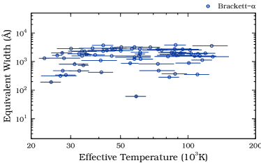
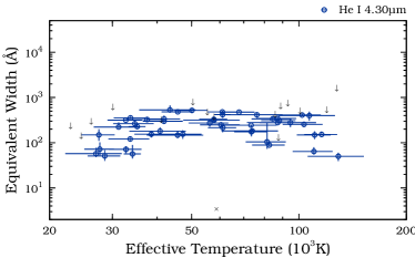
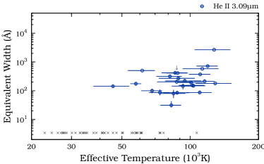
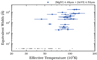
Figure 15: Equivalent widths of Brackett-$\alpha$ at 4.05$\,\mu$m (upper left), He I at 4.30$\,\mu$m (upper right), He II at 3.09$\,\mu$m (lower left), and [Mg IV] at 4.49$\,\mu$m ${+}$ [Ar VI] at 4.53$\,\mu$m (lower right) against the effective temperature. The downward arrows indicate a 3-$\sigma$ upper limit. When the emission is not detected, the effective temperature is indicated by the crosses.

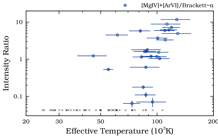
Figure 16: Intensity ratio of the summation of [Mg IV] and [Ar VI] to Brackett-$\alpha$ against the effective temperature. When the emission of [Mg IV] and [Ar VI] is not detected, the effective temperature is indicated by the crosses.

5.5 PAH Features of Galactic PNe in the Near-Infrared

The PAH features appear both in the near- and mid-infrared, and the PAH features in the mid-infrared are stronger than those in the near-infrared (e.g., Schutte et al., 1993; Draine & Li, 2001). The PAH features of PNe in the mid-infrared have been intensively investigated with Spitzer (e.g., Bernard-Salas et al., 2009; Stanghellini et al., 2007, 2012). Surveys of the 3.3$\,\mu$m PAH feature in Galactic PNe were carried out by Roche et al. (1996) and Smith & McLean (2008). Their samples were, however, biased towards carbon-rich objects. The PNSPC samples are not selected based on their chemistry. The PNSPC catalog provides a useful data set to investigate the near-infrared PAH features in Galactic PNe.

The type of dust features (carbon-rich or oxygen-rich) is thought to be closely related to the abundance ratio of nebular gas. Several studies have suggested that the intensities of the PAH features increases with the carbon-to-oxygen abundance (C/O) ratio (e.g., Cohen et al., 1986; Roche et al., 1996; Cohen & Barlow, 2005; Smith & McLean, 2008). However, PAH formation both in carbon-rich and oxygen-rich environments has been suggested recently (Guzman-Ramirez et al., 2014, 2011). Delgado-Inglada & Rodríguez (2014) measured the C/O ratio of 51 Galactic PNe and confirmed that the PAH emission can be seen even in PNe with ${\rm C/O}<1$. The C/O ratios of 11 PNe in the PNSPC catalog were measured by Delgado-Inglada & Rodríguez (2014). Figure 17 shows the equivalent width of the 3.3$\,\mu$m PAH feature against the C/O ratio. The C/O ratio measured by collisionally excited lines (CEL) is indicated by the blue circles, while that measured by recombination lines (RL) is shown by the red squares. The downward arrows indicate non-detection of the 3.3$\,\mu$m PAH features. Figure 17 shows that the 3.3$\,\mu$m PAH emission is detected even in oxygen-rich environments, consistent with Delgado-Inglada & Rodríguez (2014). Due to the small number of samples, however, it is difficult to claim the correlation between the strength of the 3.3$\,\mu$m PAH feature and the C/O ratio. Extensive measurements of the C/O ratio are encouraged.

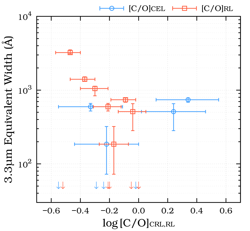
Figure 17: Equivalent width of the 3.3$\,\mu$m PAH feature against the carbon-to-oxygen (C/O) ratio. The C/O ratios are from Delgado-Inglada & Rodríguez (2014). The C/O ratio measured by collisionally excited lines (CEL) is shown by the blue circles, while the C/O ratio measured by recombination lines (RL) is by the red squares. The arrows indicate the non-detection of the 3.3$\,\mu$m PAH feature.

Figure 18 shows a cumulative histogram of the signal-to-noise ratio of the 3.3$\,\mu$m PAH feature (hereafter, ${\rm S/N}(I_{3.3})$). The gray dotted line shows the 35th percentile, which corresponds to ${\rm S/N}(I_{3.3})=3$. The result suggests that about 65% of the PNSPC samples show band emission at 3.3$\,\mu$m. The 5–38$\,\mu$m spectra of Galactic PNe with Spitzer/IRS are available in Stanghellini et al. (2012). We counted the number of PNe with PAH features, obtaining 40% (60 of 150 PNe). Despite the intrinsic weakness of the near-infrared PAH features, the PAH detection rate is as high in the near-infrared as in the mid-infrared. The 3.3$\,\mu$m feature is thought to come from the smallest PAH populations, which are most fragile, and thus primarily reflect environment variations (Schutte et al., 1993; Micelotta et al., 2010; Allain et al., 1996b, a). The PNSPC catalog is useful to investigate the evolution of the PAH features and the processing of PAHs in circumstellar environments.

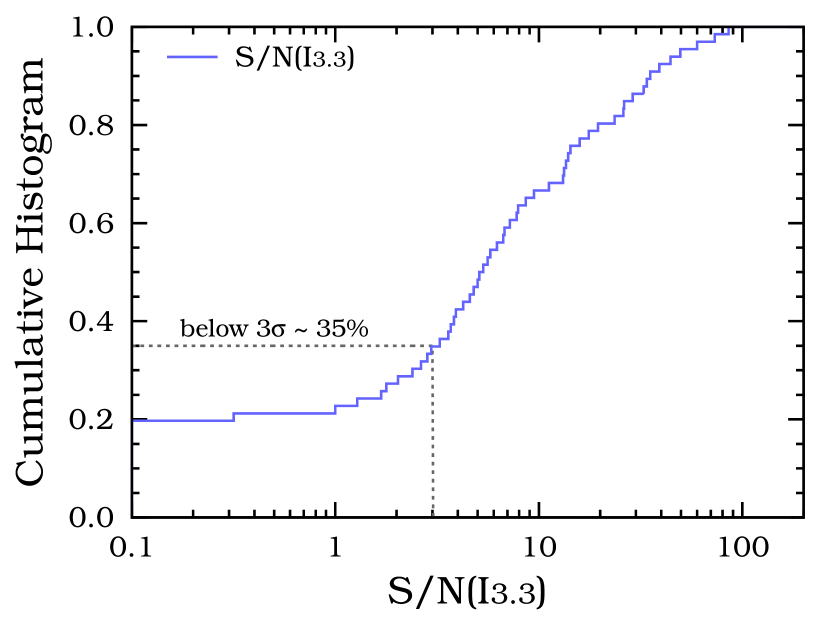
Figure 18: Cumulative histogram of the signal-to-noise ratio of the 3.3$\,\mu$m PAH feature $\left({\rm S/N}(I_{3.3})\right)$. The gray dotted-line shows the 35th percentile, which is the non-detection rate of the 3.3$\,\mu$m PAH feature when the detection limit is defined as ${\rm S/N}(I_{3.3})\geq 3$.

6 Summary & Conclusion

Near-infrared (2.5–5.0$\,\mu$m) spectra of 72 Galactic PNe were obtained at high sensitivity using the AKARI/IRC. The PNSPC program provided a set of near-infrared spectra that collected all of the flux from the objects. The absolute flux of spectra provided by the PNSPC program is in agreement with the WISE W1 photometry within ${\sim}20$%. These spectra were compiled into the PNSPC catalog. The intensity and equivalent width of Brackett-$\alpha$, He I at 4.30$\,\mu$m, He II at 3.09$\,\mu$m, the $3.3\,\mu$m PAH feature, the 3.4–3.5$\,\mu$m aliphatic feature complex, [Mg IV] at $4.49\,\mu$m, and [Ar VI] at $4.53\,\mu$m were measured. The detection limit of the emission features was as faint as $2{\times}10^{-16}\,{\rm W\,m^{-2}}$. The PNSPC catalog is the largest data set of near-infrared spectra of Galactic PNe. It provides unique information for the investigation of 2.5–5.0$\,\mu$m emission of Galactic PNe.

The Galactic coordinates of the PNSPC samples suggest that the objects in the PNSPC catalog are biased toward PNe in the Galactic disk rather than those in the Galactic bulge. The median of the effective temperature of the PNSPC samples is lower than that of the whole Galactic PNe by about 30,000 K. This indicates that the PNSPC catalog is biased toward young PNe. This bias possibly originates in the criterion on the apparent size in the target selection.

The PNSPC catalog also provides the extinction toward the objects. Even after the contribution from the interstellar medium is taken into account, Figure 13 suggests that 40% of PNe have extinction at the $V$-band larger than unity, which is attributed to the extinction in the circumstellar envelope. The present result suggests that for a large fraction of PNe a circumstellar envelope is optically thick in the UV.

The equivalent width of Brakett-$\alpha$ does not show a clear dependence on the effective temperature. The variations in the He I and He II equivalent widths can be attributed to the ionization balance between ${\rm He}^{+}$ and ${\rm He}^{++}$. The [Mg IV] at 4.49$\,\mu$m and [Ar VI] at 4.53$\,\mu$m lines are only detected when the effective temperature becomes higher than 50 000 K. The [Mg IV] and [Ar VI] lines are good indicators of PNe with a hot central star.

The 3.3$\,\mu$m PAH feature is detected in about 65% of the PNSPC samples. This detection rate is comparable to that reported from mid-infrared observations (Stanghellini et al., 2012). The present result suggests that the AKARI/IRC is as sensitive as the Spitzer/IRS in terms of detecting the PAH features. The PNSPC catalog provides a suitable data set to investigate PAHs in circumstellar environments. The near-infrared PAH features are attributed to small-sized PAHs, which are sensitive to harsh environments and processed faster than larger ones. The processing and evolution of PAHs during the PN phase will be discussed in the forth-coming paper.

Table 2: Miscellaneous Information of Objects

PN G	$V^{(a)}$	$K_{s}^{(b)}$	$A_{V}({\rm H\beta})$	$A_{V}({\rm fit.})$	$T_{\rm eff}$	Refs. $T_{\rm eff}$
	mag.	mag.	mag.	mag.	$10^{3}\,$K
000.3${+}$12.2	$\phantom{0}13.9$	$\phantom{0}11.4$	$\phantom{0}\phantom{0}0.90_{{-}0.03}^{{+}0.03}$	$\phantom{0}\phantom{0}0.98_{{-}0.05}^{{+}0.15}$	$\phantom{0}47$	Ka76,Ph03
002.0${-}$13.4	$\phantom{0}14.1$	$\phantom{0}11.1$	$\phantom{0}\phantom{0}0.31_{{-}0.01}^{{+}0.02}$	$\phantom{0}\phantom{0}0.38_{{-}0.04}^{{+}0.02}$	$\phantom{0}60$	PM89,PM91,Ph03
003.1${+}$02.9	${>}17.0$	$\phantom{0}11.6$	$\phantom{0}\phantom{0}3.31_{{-}0.03}^{{+}0.03}$	$\phantom{0}\phantom{0}\phantom{0}3.4_{{-}0.1}^{{+}0.6}$	$\phantom{0}87$	PM89,Ph03
011.0${+}$05.8	$\cdots$	$\phantom{0}11.8$	$\phantom{0}\phantom{0}1.81_{{-}0.04}^{{+}0.04}$	$\phantom{0}\phantom{0}1.79_{{-}0.06}^{{+}0.06}$	$\phantom{0}93$	PM91,Ph03
027.6${-}$09.6	$\phantom{0}15.2$	$\phantom{0}11.9$	$\phantom{0}\phantom{0}1.04_{{-}0.05}^{{+}0.06}$	$\phantom{0}\phantom{0}\phantom{0}1.0_{{-}0.2}^{{+}0.9}$	$\phantom{0}58$	PM91,Ka76,KJ91,Ph03
037.8${-}$06.3	$\cdots$	$\phantom{0}9.47$	$\phantom{0}\phantom{0}\phantom{0}1.4_{{-}0.1}^{{+}0.1}$	$\phantom{0}\phantom{0}1.41_{{-}0.02}^{{+}0.08}$	$\phantom{0}74$	Ph03
038.2${+}$12.0	$\phantom{0}12.5$	$\phantom{0}11.1$	$\phantom{0}\phantom{0}0.82_{{-}0.05}^{{+}0.05}$	$\phantom{0}\phantom{0}0.93_{{-}0.07}^{{+}0.07}$	$\phantom{0}30$	Ka78,Ph03
043.1${+}$03.8	$\phantom{0}14.9$	$\phantom{0}12.1$	$\phantom{0}\phantom{0}\phantom{0}1.9_{{-}0.1}^{{+}0.1}$	$\phantom{0}\phantom{0}2.05_{{-}0.05}^{{+}0.46}$	$\phantom{0}28$	Ph03
046.4${-}$04.1	$\phantom{0}15.2$	$\phantom{0}11.1$	$\phantom{0}\phantom{0}1.42_{{-}0.02}^{{+}0.02}$	$\phantom{0}\phantom{0}1.39_{{-}0.01}^{{+}0.01}$	$\phantom{0}68$	Ka76,KJ91,Ph03
051.4${+}$09.6	$\phantom{0}13.3$	$\phantom{0}10.4$	$\phantom{0}\phantom{0}0.88_{{-}0.04}^{{+}0.05}$	$\phantom{0}\phantom{0}0.98_{{-}0.08}^{{+}0.11}$	$\phantom{0}37$	Ka76,Ka78,Ph03
052.2${-}$04.0	$\phantom{0}18.1$	$\phantom{0}12.0$	$\phantom{0}\phantom{0}1.68_{{-}0.04}^{{+}0.05}$	$\phantom{0}\phantom{0}1.62_{{-}0.09}^{{+}0.09}$	$\phantom{0}61$	Lu01,PM89,KJ91,Ph03
058.3${-}$10.9	$\phantom{0}14.4$	$\phantom{0}9.67$	$\phantom{0}\phantom{0}0.66_{{-}0.05}^{{+}0.05}$	$\phantom{0}\phantom{0}0.18_{{-}0.04}^{{+}0.08}$	$\phantom{0}50$	PM89,Ka76,Ph03
060.1${-}$07.7	$\phantom{0}18.0$	$\phantom{0}11.5$	$\phantom{0}\phantom{0}1.19_{{-}0.02}^{{+}0.02}$	$\phantom{0}\phantom{0}1.28_{{-}0.02}^{{+}0.03}$	$129$	Ph03
060.5${+}$01.8	$\cdots$	$\phantom{0}11.8$	$\phantom{0}\phantom{0}\phantom{0}4.1_{{-}0.2}^{{+}0.2}$	$\phantom{0}\phantom{0}\phantom{0}3.5_{{-}0.4}^{{+}0.5}$	$\cdots$	$\cdots$
064.7${+}$05.0	$\phantom{0}12.5$	$\phantom{0}8.11$	$\phantom{0}\phantom{0}1.44_{{-}0.04}^{{+}0.04}$	$\phantom{0}\phantom{0}1.43_{{-}0.04}^{{+}0.05}$	$\phantom{0}28$	Lu01,Ka76,Ka78,Ph03
071.6${-}$02.3	${>}15.7$	$\phantom{0}10.1$	$\phantom{0}\phantom{0}\phantom{0}4.4_{{-}0.1}^{{+}0.1}$	$\phantom{0}\phantom{0}\phantom{0}5.1_{{-}0.7}^{{+}1.3}$	$\cdots$	$\cdots$
074.5${+}$02.1	$\phantom{0}18.4$	$\phantom{0}11.0$	$\phantom{0}\phantom{0}3.43_{{-}0.07}^{{+}0.07}$	$\phantom{0}\phantom{0}3.47_{{-}0.04}^{{+}1.32}$	$\phantom{0}81$	Ph03
082.1${+}$07.0	${>}15.6$	$\phantom{0}10.7$	$\phantom{0}\phantom{0}1.71_{{-}0.08}^{{+}0.07}$	$\phantom{0}\phantom{0}\phantom{0}1.7_{{-}0.1}^{{+}2.3}$	$\phantom{0}87$	Ph03
082.5${+}$11.3	$\phantom{0}14.5$	$\phantom{0}12.2$	$\phantom{0}\phantom{0}0.17_{{-}0.04}^{{+}0.04}$	$\phantom{0}\phantom{0}0.16_{{-}0.05}^{{+}0.08}$	$\phantom{0}63$	Me88
086.5${-}$08.8	$\phantom{0}17.3$	$\phantom{0}12.5$	$\phantom{0}\phantom{0}0.60_{{-}0.03}^{{+}0.03}$	$\phantom{0}\phantom{0}0.52_{{-}0.03}^{{+}0.03}$	$\phantom{0}61$	Lu01,Ph03
089.3${-}$02.2	$\phantom{0}12.1$	$\phantom{0}9.20$	$\phantom{0}\phantom{0}\phantom{0}2.0_{{-}0.5}^{{+}0.8}$	$\phantom{0}\phantom{0}1.90_{{-}0.01}^{{+}5.40}$	$\cdots$	$\cdots$
089.8${-}$05.1	$\phantom{0}16.7$	$\phantom{0}9.49$	$\phantom{0}\phantom{0}1.99_{{-}0.04}^{{+}0.04}$	$\phantom{0}\phantom{0}2.02_{{-}0.01}^{{+}0.02}$	$\phantom{0}83$	Ka78,KJ91,Ph03
095.2${+}$00.7	$\cdots$	$\phantom{0}11.2$	$\phantom{0}\phantom{0}\phantom{0}5.5_{{-}0.2}^{{+}0.3}$	$\phantom{0}\phantom{0}\phantom{0}5.4_{{-}0.1}^{{+}0.4}$	$\phantom{0}58$	Lu01
100.6${-}$05.4	$\phantom{0}15.5$	$\phantom{0}12.0$	$\phantom{0}\phantom{0}0.52_{{-}0.03}^{{+}0.03}$	$\phantom{0}\phantom{0}0.47_{{-}0.07}^{{+}0.05}$	$\phantom{0}74$	Ka78,KJ91,Ph03
111.8${-}$02.8	$\phantom{0}13.8$	$\phantom{0}8.81$	$\phantom{0}\phantom{0}1.92_{{-}0.10}^{{+}0.10}$	$\phantom{0}\phantom{0}2.12_{{-}0.76}^{{+}0.01}$	$\phantom{0}41$	Ka76,Ph03
118.0${-}$08.6	$\phantom{0}14.2$	$\phantom{0}12.9$	$\phantom{0}\phantom{0}0.41_{{-}0.10}^{{+}0.10}$	$\phantom{0}\phantom{0}0.32_{{-}0.03}^{{+}0.02}$	$\phantom{0}55$	Lu01,Ka76,KJ91,Ph03
123.6${+}$34.5	$\phantom{0}13.4$	$\phantom{0}11.9$	$\phantom{0}\phantom{0}0.50_{{-}0.03}^{{+}0.03}$	$\phantom{0}\phantom{0}0.60_{{-}0.03}^{{+}0.09}$	$\phantom{0}50$	HF83
146.7${+}$07.6	$\phantom{0}14.0$	$\phantom{0}11.2$	$\phantom{0}\phantom{0}1.55_{{-}0.09}^{{+}0.09}$	$\phantom{0}\phantom{0}1.56_{{-}0.02}^{{+}0.29}$	$\phantom{0}27$	Ph03
159.0${-}$15.1	$\phantom{0}15.8$	$\phantom{0}12.6$	$\phantom{0}\phantom{0}0.44_{{-}0.04}^{{+}0.04}$	$\phantom{0}\phantom{0}0.40_{{-}0.06}^{{+}0.02}$	$\phantom{0}89$	Ph03
166.1${+}$10.4	$\phantom{0}11.6$	$\phantom{0}10.6$	$\phantom{0}\phantom{0}0.63_{{-}0.02}^{{+}0.02}$	$\phantom{0}\phantom{0}0.64_{{-}0.03}^{{+}0.02}$	$\phantom{0}39$	Ka76,Ka78,Ph03
190.3${-}$17.7	$\phantom{0}14.4$	$\phantom{0}13.2$	$\phantom{0}\phantom{0}0.34_{{-}0.03}^{{+}0.03}$	$\phantom{0}\phantom{0}0.36_{{-}0.04}^{{+}0.10}$	$\phantom{0}61$	PM89,Ka76,KJ91,Ph03
194.2${+}$02.5	$\phantom{0}17.8$	$\phantom{0}10.6$	$\phantom{0}\phantom{0}1.40_{{-}0.06}^{{+}0.06}$	$\phantom{0}\phantom{0}1.41_{{-}0.12}^{{+}0.04}$	$\phantom{0}88$	PM89,Ph03
211.2${-}$03.5	$\phantom{0}15.8$	$\phantom{0}10.6$	$\phantom{0}\phantom{0}\phantom{0}3.5_{{-}0.2}^{{+}0.2}$	$\phantom{0}\phantom{0}3.49_{{-}0.02}^{{+}0.03}$	$\phantom{0}33$	Lu01,PM89,Ph03
221.3${-}$12.3	$\phantom{0}17.9$	$\phantom{0}11.0$	$\phantom{0}\phantom{0}0.91_{{-}0.01}^{{+}0.01}$	$\phantom{0}\phantom{0}0.91_{{-}0.02}^{{+}0.10}$	$111$	PM91,Ph03
226.7${+}$05.6	$\phantom{0}16.9$	$\phantom{0}12.8$	$\phantom{0}\phantom{0}1.63_{{-}0.03}^{{+}0.02}$	$\phantom{0}\phantom{0}1.61_{{-}0.05}^{{+}0.11}$	$\phantom{0}46$	Ph03
232.8${-}$04.7	$\phantom{0}13.9$	$\phantom{0}9.48$	$\phantom{0}\phantom{0}2.96_{{-}0.06}^{{+}0.06}$	$\phantom{0}\phantom{0}2.99_{{-}0.09}^{{+}0.39}$	$\phantom{0}25$	Lu01,PM89,Ph03
235.3${-}$03.9	$\phantom{0}14.1$	$\phantom{0}10.6$	$\phantom{0}\phantom{0}\phantom{0}1.6_{{-}0.2}^{{+}0.2}$	$\phantom{0}\phantom{0}1.62_{{-}0.01}^{{+}0.01}$	$\phantom{0}29$	Lu01,PM89,Ph03
258.1${-}$00.3	$\phantom{0}16.2$	$\phantom{0}10.9$	$\phantom{0}\phantom{0}4.02_{{-}0.03}^{{+}0.03}$	$\phantom{0}\phantom{0}4.02_{{-}0.04}^{{+}0.05}$	$\phantom{0}60$	PM91,Ph03
264.4${-}$12.7	$\phantom{0}14.7$	$\phantom{0}12.2$	$\phantom{0}\phantom{0}0.72_{{-}0.07}^{{+}0.07}$	$\phantom{0}\phantom{0}\phantom{0}0.6_{{-}0.1}^{{+}0.1}$	$\phantom{0}56$	PM91,KJ91
268.4${+}$02.4	$\phantom{0}18.7$	$\phantom{0}10.6$	$\phantom{0}\phantom{0}3.80_{{-}0.03}^{{+}0.03}$	$\phantom{0}\phantom{0}3.91_{{-}0.05}^{{+}0.23}$	$110$	PM91,Ph03
278.6${-}$06.7	$\cdots$	$\phantom{0}12.3$	$\phantom{0}\phantom{0}0.73_{{-}0.03}^{{+}0.03}$	$\phantom{0}\phantom{0}0.75_{{-}0.05}^{{+}0.10}$	$\phantom{0}84$	PM91,Ph03
283.8${+}$02.2	$\phantom{0}17.2$	$\phantom{0}12.3$	$\phantom{0}\phantom{0}1.57_{{-}0.02}^{{+}0.02}$	$\phantom{0}\phantom{0}1.35_{{-}0.01}^{{+}0.01}$	$113$	Ph03
285.4${-}$05.3	$\phantom{0}15.5$	$\phantom{0}11.6$	$\phantom{0}\phantom{0}0.75_{{-}0.02}^{{+}0.03}$	$\phantom{0}\phantom{0}0.68_{{-}0.01}^{{+}0.03}$	$100$	PM91,Ph03
285.6${-}$02.7	$\phantom{0}13.0$	$\phantom{0}10.2$	$\phantom{0}\phantom{0}2.11_{{-}0.02}^{{+}0.02}$	$\phantom{0}\phantom{0}2.16_{{-}0.05}^{{+}0.06}$	$\phantom{0}34$	PM89,Ph03
285.7${-}$14.9	$\phantom{0}14.2$	$\phantom{0}13.3$	$\phantom{0}\phantom{0}0.14_{{-}0.03}^{{+}0.03}$	$\phantom{0}\phantom{0}0.14_{{-}0.03}^{{+}0.02}$	$\phantom{0}55$	Me88
291.6${-}$04.8	$\phantom{0}15.4$	$\phantom{0}10.5$	$\phantom{0}\phantom{0}1.80_{{-}0.02}^{{+}0.02}$	$\phantom{0}\phantom{0}1.79_{{-}0.03}^{{+}0.13}$	$116$	PM91,Ph03
292.8${+}$01.1	$\cdots$	$\phantom{0}12.5$	$\phantom{0}\phantom{0}2.03_{{-}0.03}^{{+}0.02}$	$\phantom{0}\phantom{0}2.16_{{-}0.07}^{{+}0.19}$	$\phantom{0}95$	PM91
294.9${-}$04.3	$\cdots$	$\phantom{0}11.5$	$\phantom{0}\phantom{0}1.80_{{-}0.02}^{{+}0.02}$	$\phantom{0}\phantom{0}1.80_{{-}0.05}^{{+}0.08}$	$\phantom{0}41$	PM89
296.3${-}$03.0	$\phantom{0}16.1$	$\phantom{0}11.6$	$\phantom{0}\phantom{0}2.32_{{-}0.05}^{{+}0.05}$	$\phantom{0}\phantom{0}2.38_{{-}0.06}^{{+}0.35}$	$103$	PM91,Ph03
304.5${-}$04.8	$\phantom{0}16.4$	$\phantom{0}10.8$	$\phantom{0}\phantom{0}1.34_{{-}0.04}^{{+}0.04}$	$\phantom{0}\phantom{0}1.34_{{-}0.02}^{{+}0.05}$	$102$	PM91,Ph03
305.1${+}$01.4	$\phantom{0}15.6$	$\phantom{0}7.93$	$\phantom{0}\phantom{0}\phantom{0}3.5_{{-}0.1}^{{+}0.1}$	$\phantom{0}\phantom{0}3.50_{{-}0.05}^{{+}0.02}$	$\phantom{0}59$	PM91,KJ91,Ph03
307.2${-}$09.0	$\phantom{0}15.3$	$\phantom{0}11.6$	$\phantom{0}\phantom{0}1.16_{{-}0.02}^{{+}0.02}$	$\phantom{0}\phantom{0}1.10_{{-}0.03}^{{+}0.05}$	$\phantom{0}50$	PM89,KJ91,Ph03
307.5${-}$04.9	$\cdots$	$\phantom{0}10.8$	$\phantom{0}\phantom{0}\phantom{0}1.6_{{-}0.1}^{{+}0.2}$	$\phantom{0}\phantom{0}1.64_{{-}0.03}^{{+}0.07}$	$\phantom{0}38$	PM89,Ph03
312.6${-}$01.8	$\phantom{0}15.1$	$\phantom{0}11.9$	$\phantom{0}\phantom{0}3.17_{{-}0.03}^{{+}0.03}$	$\phantom{0}\phantom{0}3.35_{{-}0.08}^{{+}0.47}$	$\phantom{0}42$	PM89,KJ91,Ph03
315.1${-}$13.0	$\phantom{0}11.0$	$\phantom{0}9.36$	$\phantom{0}\phantom{0}\phantom{0}0.5_{{-}0.1}^{{+}0.1}$	$\phantom{0}\phantom{0}\phantom{0}\phantom{0}\phantom{0}9_{{-}5}^{{+}1}$	$\phantom{0}27$	PM89,Ka78,Ph03
320.1${-}$09.6	$\phantom{0}10.9$	$\phantom{0}10.1$	$\phantom{0}\phantom{0}0.72_{{-}0.07}^{{+}0.08}$	$\phantom{0}\phantom{0}0.63_{{-}0.05}^{{+}3.31}$	$\phantom{0}27$	Me88
320.9${+}$02.0	${>}17.9$	$\phantom{0}10.2$	$\phantom{0}\phantom{0}4.96_{{-}0.09}^{{+}0.09}$	$\phantom{0}\phantom{0}\phantom{0}\phantom{0}\phantom{0}7_{{-}2}^{{+}2}$	$\phantom{0}44$	PM89
322.5${-}$05.2	$\phantom{0}15.3$	$\phantom{0}12.7$	$\phantom{0}\phantom{0}0.80_{{-}0.03}^{{+}0.03}$	$\phantom{0}\phantom{0}0.89_{{-}0.04}^{{+}0.19}$	$127$	Ph03
323.9${+}$02.4	$\phantom{0}16.8$	$\phantom{0}11.8$	$\phantom{0}\phantom{0}3.05_{{-}0.03}^{{+}0.03}$	$\phantom{0}\phantom{0}3.01_{{-}0.22}^{{+}0.05}$	$\phantom{0}42$	PM89,Ph03
324.8${-}$01.1	$\cdots$	$\phantom{0}10.6$	$\phantom{0}\phantom{0}6.34_{{-}0.03}^{{+}0.02}$	$\phantom{0}\phantom{0}\phantom{0}6.5_{{-}0.2}^{{+}0.3}$	$\cdots$	$\cdots$
325.8${-}$12.8	$\phantom{0}13.4$	$\phantom{0}11.1$	$\phantom{0}\phantom{0}0.50_{{-}0.03}^{{+}0.03}$	$\phantom{0}\phantom{0}\phantom{0}0.9_{{-}0.1}^{{+}0.5}$	$\phantom{0}36$	Me88
326.0${-}$06.5	$\phantom{0}13.1$	$\phantom{0}11.8$	$\phantom{0}\phantom{0}1.23_{{-}0.07}^{{+}0.07}$	$\phantom{0}\phantom{0}1.16_{{-}0.05}^{{+}0.04}$	$\phantom{0}25$	Me88
327.1${-}$01.8	$\phantom{0}17.2$	$\phantom{0}11.5$	$\phantom{0}\phantom{0}3.83_{{-}0.03}^{{+}0.04}$	$\phantom{0}\phantom{0}\phantom{0}4.2_{{-}0.3}^{{+}0.2}$	$\phantom{0}35$	PM89,Ph03
327.8${-}$01.6	$\cdots$	$\phantom{0}11.0$	$\phantom{0}\phantom{0}5.10_{{-}0.03}^{{+}0.03}$	$\phantom{0}\phantom{0}\phantom{0}5.7_{{-}0.5}^{{+}0.7}$	$\cdots$	$\cdots$
331.1${-}$05.7	$\phantom{0}12.7$	$\phantom{0}10.3$	$\phantom{0}\phantom{0}\phantom{0}1.4_{{-}0.1}^{{+}0.1}$	$\phantom{0}\phantom{0}1.36_{{-}0.03}^{{+}3.35}$	$\phantom{0}31$	PM89,Ph03
331.3${+}$16.8	$\phantom{0}15.5$	$\phantom{0}12.5$	$\phantom{0}\phantom{0}0.10_{{-}0.03}^{{+}0.03}$	$\phantom{0}\phantom{0}0.78_{{-}0.46}^{{+}0.01}$	$\phantom{0}86$	PM89,Ph03
336.3${-}$05.6	$\phantom{0}16.6$	$\phantom{0}12.2$	$\phantom{0}\phantom{0}1.32_{{-}0.06}^{{+}0.07}$	$\phantom{0}\phantom{0}1.36_{{-}0.03}^{{+}0.02}$	$101$	PM91,Ph03
342.1${+}$27.5	$\cdots$	$\phantom{0}13.2$	$\phantom{0}\phantom{0}0.25_{{-}0.02}^{{+}0.02}$	$\phantom{0}\phantom{0}0.27_{{-}0.04}^{{+}0.47}$	$119$	PM89,Ph03
349.8${+}$04.4	$\phantom{0}17.0$	$\phantom{0}12.1$	$\phantom{0}\phantom{0}\phantom{0}1.9_{{-}0.1}^{{+}0.2}$	$\phantom{0}\phantom{0}\phantom{0}2.1_{{-}0.1}^{{+}0.1}$	$\phantom{0}76$	PM89
350.9${+}$04.4	$\phantom{0}13.3$	$\phantom{0}10.3$	$\phantom{0}\phantom{0}1.83_{{-}0.08}^{{+}0.07}$	$\phantom{0}\phantom{0}1.83_{{-}0.02}^{{+}2.23}$	$\phantom{0}33$	Me88
356.1${+}$02.7	$\cdots$	$\phantom{0}11.9$	$\phantom{0}\phantom{0}\phantom{0}5.8_{{-}0.5}^{{+}1.0}$	$\phantom{0}\phantom{0}5.54_{{-}0.01}^{{+}0.16}$	$\phantom{0}73$	PM89
357.6${+}$02.6	$\cdots$	$\phantom{0}12.2$	$\phantom{0}\phantom{0}\phantom{0}4.7_{{-}0.6}^{{+}1.8}$	$\phantom{0}\phantom{0}4.71_{{-}0.45}^{{+}0.06}$	$107$	PM91

References. — ^(a)Acker et al. (1992); ^(b) Skrutskie et al. (2006); HF83: Harrington & Feibelman (1983), Ka76: Kaler (1976), Ka78: Kaler (1978), KJ91: Kaler & Jacoby (1991), Lu01: Lumsden et al. (2001), Me88: Mendez et al. (1988), Ph03: Phillips (2003), PM89: Preite-Martinez et al. (1989), PM91: Preite-Martinez et al. (1991).

Table 5: Extinction Corrected Line Intensity

PN G	Bracket-$\alpha$	He II$(3.09{\rm\mu m})$	He I$(4.30{\rm\mu m})$	PAH$(3.3{\rm\mu m})$	C−Hal$(3.4$-$3.5{\rm\mu m})$	[Mg IV]$(4.49{\rm\mu m})$	[Ar VI]$(4.53{\rm\mu m})$
	$10^{-15}\,{\rm W\,m^{-2}}$	$10^{-15}\,{\rm W\,m^{-2}}$	$10^{-15}\,{\rm W\,m^{-2}}$	$10^{-15}\,{\rm W\,m^{-2}}$	$10^{-15}\,{\rm W\,m^{-2}}$	$10^{-15}\,{\rm W\,m^{-2}}$	$10^{-15}\,{\rm W\,m^{-2}}$
000.3${+}$12.2	$\phantom{0}\phantom{0}\phantom{0}2.74_{{-}0.04}^{{+}0.05}$	$\cdots$	$\phantom{0}\phantom{0}\phantom{0}0.14_{{-}0.03}^{{+}0.03}$	${<}0.11$	$\cdots$	$\cdots$	$\cdots$
002.0${-}$13.4	$\phantom{0}\phantom{0}\phantom{0}2.05_{{-}0.03}^{{+}0.04}$	$\cdots$	$\phantom{0}\phantom{0}\phantom{0}0.31_{{-}0.02}^{{+}0.03}$	$\phantom{0}\phantom{0}\phantom{0}0.25_{{-}0.05}^{{+}0.05}$	${<}0.10$	$\cdots$	$\cdots$
003.1${+}$02.9	$\phantom{0}\phantom{0}\phantom{0}3.16_{{-}0.04}^{{+}0.04}$	${<}0.53$	$\phantom{0}\phantom{0}\phantom{0}0.43_{{-}0.04}^{{+}0.03}$	$\phantom{0}\phantom{0}\phantom{0}0.94_{{-}0.16}^{{+}0.25}$	$\phantom{0}\phantom{0}\phantom{0}0.49_{{-}0.08}^{{+}0.09}$	$\phantom{0}\phantom{0}\phantom{0}0.35_{{-}0.04}^{{+}0.05}$	$\cdots$
011.0${+}$05.8	$\phantom{0}\phantom{0}\phantom{0}1.09_{{-}0.04}^{{+}0.03}$	$\phantom{0}\phantom{0}\phantom{0}0.13_{{-}0.03}^{{+}0.03}$	${<}0.13$	$\cdots$	$\cdots$	$\phantom{0}\phantom{0}\phantom{0}1.11_{{-}0.08}^{{+}0.05}$	$\phantom{0}\phantom{0}\phantom{0}0.20_{{-}0.05}^{{+}0.04}$
027.6${-}$09.6	$\phantom{0}\phantom{0}\phantom{0}1.12_{{-}0.02}^{{+}0.04}$	$\cdots$	$\phantom{0}\phantom{0}\phantom{0}0.10_{{-}0.01}^{{+}0.01}$	$\cdots$	$\cdots$	$\cdots$	$\cdots$
037.8${-}$06.3	$\phantom{0}\phantom{0}\phantom{0}4.61_{{-}0.10}^{{+}0.24}$	$\cdots$	$\phantom{0}\phantom{0}\phantom{0}1.80_{{-}0.09}^{{+}0.13}$	$\phantom{0}\phantom{0}\phantom{0}6.64_{{-}0.21}^{{+}0.40}$	$\phantom{0}\phantom{0}\phantom{0}2.60_{{-}0.14}^{{+}0.21}$	$\cdots$	$\cdots$
038.2${+}$12.0	$\phantom{0}\phantom{0}\phantom{0}2.18_{{-}0.06}^{{+}0.04}$	$\cdots$	${<}0.13$	$\phantom{0}\phantom{0}\phantom{0}0.45_{{-}0.05}^{{+}0.04}$	$\phantom{0}\phantom{0}\phantom{0}0.12_{{-}0.02}^{{+}0.03}$	$\cdots$	$\cdots$
043.1${+}$03.8	$\phantom{0}\phantom{0}\phantom{0}0.45_{{-}0.01}^{{+}0.01}$	$\cdots$	$\cdots$	${<}0.06$	${<}0.01$	$\cdots$	$\cdots$
046.4${-}$04.1	$\phantom{0}\phantom{0}\phantom{0}2.43_{{-}0.01}^{{+}0.02}$	$\phantom{0}\phantom{0}\phantom{0}0.11_{{-}0.02}^{{+}0.02}$	$\phantom{0}\phantom{0}\phantom{0}0.32_{{-}0.01}^{{+}0.02}$	$\phantom{0}\phantom{0}\phantom{0}0.40_{{-}0.05}^{{+}0.04}$	${<}0.16$	$\cdots$	$\cdots$
051.4${+}$09.6	$\phantom{0}\phantom{0}\phantom{0}3.25_{{-}0.02}^{{+}0.06}$	$\cdots$	$\phantom{0}\phantom{0}\phantom{0}0.52_{{-}0.02}^{{+}0.02}$	$\phantom{0}\phantom{0}\phantom{0}0.97_{{-}0.07}^{{+}0.05}$	$\phantom{0}\phantom{0}\phantom{0}0.23_{{-}0.05}^{{+}0.04}$	$\cdots$	$\cdots$
052.2${-}$04.0	$\phantom{0}\phantom{0}\phantom{0}0.87_{{-}0.01}^{{+}0.01}$	$\cdots$	$\phantom{0}\phantom{0}\phantom{0}0.14_{{-}0.01}^{{+}0.01}$	$\phantom{0}\phantom{0}\phantom{0}0.05_{{-}0.01}^{{+}0.01}$	${<}0.03$	$\cdots$	$\cdots$
058.3${-}$10.9	$\phantom{0}\phantom{0}\phantom{0}4.62_{{-}0.07}^{{+}0.10}$	$\cdots$	$\phantom{0}\phantom{0}\phantom{0}0.99_{{-}0.04}^{{+}0.07}$	${<}0.55$	${<}0.26$	$\cdots$	$\cdots$
060.1${-}$07.7	$\phantom{0}\phantom{0}\phantom{0}1.41_{{-}0.01}^{{+}0.02}$	$\phantom{0}\phantom{0}\phantom{0}0.19_{{-}0.01}^{{+}0.01}$	$\phantom{0}\phantom{0}\phantom{0}0.05_{{-}0.01}^{{+}0.01}$	$\phantom{0}\phantom{0}\phantom{0}2.21_{{-}0.03}^{{+}0.03}$	$\phantom{0}\phantom{0}\phantom{0}1.34_{{-}0.03}^{{+}0.03}$	$\phantom{0}\phantom{0}\phantom{0}5.04_{{-}0.06}^{{+}0.06}$	$\phantom{0}\phantom{0}\phantom{0}1.90_{{-}0.03}^{{+}0.04}$
060.5${+}$01.8	$\phantom{0}\phantom{0}\phantom{0}1.12_{{-}0.01}^{{+}0.03}$	$\cdots$	$\phantom{0}\phantom{0}\phantom{0}0.16_{{-}0.01}^{{+}0.01}$	$\phantom{0}\phantom{0}\phantom{0}0.23_{{-}0.04}^{{+}0.02}$	$\phantom{0}\phantom{0}\phantom{0}0.07_{{-}0.02}^{{+}0.01}$	$\cdots$	$\cdots$
064.7${+}$05.0	$\phantom{0}\phantom{0}34.69_{{-}1.38}^{{+}1.49}$	$\cdots$	$\phantom{0}\phantom{0}\phantom{0}5.17_{{-}1.38}^{{+}2.18}$	$\phantom{0}145.36_{{-}4.23}^{{+}4.77}$	$\phantom{0}\phantom{0}50.92_{{-}1.79}^{{+}2.87}$	$\cdots$	$\cdots$
071.6${-}$02.3	$\phantom{0}\phantom{0}\phantom{0}3.50_{{-}0.09}^{{+}0.22}$	$\cdots$	$\phantom{0}\phantom{0}\phantom{0}0.75_{{-}0.09}^{{+}0.13}$	$\phantom{0}\phantom{0}\phantom{0}7.13_{{-}0.58}^{{+}0.37}$	$\phantom{0}\phantom{0}\phantom{0}2.07_{{-}0.44}^{{+}0.29}$	$\cdots$	$\cdots$
074.5${+}$02.1	$\phantom{0}\phantom{0}\phantom{0}1.82_{{-}0.06}^{{+}0.08}$	$\phantom{0}\phantom{0}\phantom{0}0.41_{{-}0.03}^{{+}0.06}$	$\phantom{0}\phantom{0}\phantom{0}0.12_{{-}0.04}^{{+}0.20}$	$\phantom{0}\phantom{0}\phantom{0}2.86_{{-}0.22}^{{+}0.25}$	$\phantom{0}\phantom{0}\phantom{0}1.68_{{-}0.10}^{{+}0.37}$	$\phantom{0}\phantom{0}\phantom{0}4.43_{{-}0.25}^{{+}0.39}$	$\phantom{0}\phantom{0}\phantom{0}6.18_{{-}0.34}^{{+}0.30}$
082.1${+}$07.0	$\phantom{0}\phantom{0}\phantom{0}3.85_{{-}0.04}^{{+}0.40}$	$\phantom{0}\phantom{0}\phantom{0}0.40_{{-}0.02}^{{+}0.08}$	$\phantom{0}\phantom{0}\phantom{0}0.34_{{-}0.02}^{{+}0.06}$	$\cdots$	$\cdots$	$\phantom{0}\phantom{0}\phantom{0}2.25_{{-}0.06}^{{+}0.09}$	$\phantom{0}\phantom{0}\phantom{0}0.10_{{-}0.02}^{{+}0.09}$
082.5${+}$11.3	$\phantom{0}\phantom{0}\phantom{0}0.52_{{-}0.02}^{{+}0.02}$	$\cdots$	$\phantom{0}\phantom{0}\phantom{0}0.10_{{-}0.02}^{{+}0.02}$	$\cdots$	$\cdots$	$\cdots$	$\cdots$
086.5${-}$08.8	$\phantom{0}\phantom{0}\phantom{0}0.92_{{-}0.01}^{{+}0.01}$	$\phantom{0}\phantom{0}\phantom{0}0.49_{{-}0.01}^{{+}0.02}$	$\cdots$	${<}0.08$	${<}0.07$	$\phantom{0}\phantom{0}\phantom{0}1.40_{{-}0.03}^{{+}0.03}$	$\phantom{0}\phantom{0}\phantom{0}2.75_{{-}0.06}^{{+}0.05}$
089.3${-}$02.2	$\phantom{0}\phantom{0}\phantom{0}0.79_{{-}0.07}^{{+}0.24}$	$\cdots$	$\cdots$	$\phantom{0}\phantom{0}\phantom{0}1.96_{{-}0.17}^{{+}0.62}$	${<}0.48$	$\cdots$	$\cdots$
089.8${-}$05.1	$\phantom{0}\phantom{0}\phantom{0}2.92_{{-}0.03}^{{+}0.15}$	$\phantom{0}\phantom{0}\phantom{0}0.23_{{-}0.04}^{{+}0.09}$	$\phantom{0}\phantom{0}\phantom{0}0.92_{{-}0.06}^{{+}0.11}$	$\phantom{0}\phantom{0}14.75_{{-}0.19}^{{+}0.41}$	$\phantom{0}\phantom{0}\phantom{0}4.86_{{-}0.09}^{{+}0.22}$	$\phantom{0}\phantom{0}\phantom{0}2.91_{{-}0.05}^{{+}0.24}$	$\phantom{0}\phantom{0}\phantom{0}0.43_{{-}0.06}^{{+}0.14}$
095.2${+}$00.7	$\phantom{0}\phantom{0}\phantom{0}2.52_{{-}0.06}^{{+}0.07}$	$\cdots$	$\phantom{0}\phantom{0}\phantom{0}0.53_{{-}0.02}^{{+}0.06}$	$\phantom{0}\phantom{0}\phantom{0}0.56_{{-}0.06}^{{+}0.08}$	${<}0.18$	$\cdots$	$\cdots$
100.6${-}$05.4	$\phantom{0}\phantom{0}\phantom{0}0.93_{{-}0.01}^{{+}0.01}$	$\phantom{0}\phantom{0}\phantom{0}0.05_{{-}0.01}^{{+}0.01}$	$\phantom{0}\phantom{0}\phantom{0}0.05_{{-}0.01}^{{+}0.01}$	$\cdots$	$\cdots$	$\phantom{0}\phantom{0}\phantom{0}0.06_{{-}0.01}^{{+}0.01}$	$\cdots$
111.8${-}$02.8	$\phantom{0}\phantom{0}\phantom{0}6.18_{{-}0.47}^{{+}0.01}$	$\cdots$	${<}2.62$	${<}3.55$	$\phantom{0}\phantom{0}\phantom{0}1.65_{{-}0.29}^{{+}0.38}$	$\cdots$	$\cdots$
118.0${-}$08.6	$\phantom{0}\phantom{0}\phantom{0}0.35_{{-}0.02}^{{+}0.02}$	$\cdots$	${<}0.05$	$\cdots$	$\cdots$	$\cdots$	$\cdots$
123.6${+}$34.5	$\phantom{0}\phantom{0}\phantom{0}2.02_{{-}0.05}^{{+}0.05}$	$\cdots$	${<}0.15$	${<}0.18$	${<}0.05$	$\cdots$	$\cdots$
146.7${+}$07.6	$\phantom{0}\phantom{0}\phantom{0}0.56_{{-}0.01}^{{+}0.04}$	$\cdots$	$\phantom{0}\phantom{0}\phantom{0}0.10_{{-}0.02}^{{+}0.03}$	$\phantom{0}\phantom{0}\phantom{0}4.23_{{-}0.10}^{{+}0.14}$	$\phantom{0}\phantom{0}\phantom{0}0.79_{{-}0.04}^{{+}0.08}$	$\cdots$	$\cdots$
159.0${-}$15.1	$\phantom{0}\phantom{0}\phantom{0}0.48_{{-}0.01}^{{+}0.01}$	$\phantom{0}\phantom{0}\phantom{0}0.11_{{-}0.01}^{{+}0.01}$	${<}0.06$	$\cdots$	$\cdots$	$\phantom{0}\phantom{0}\phantom{0}0.86_{{-}0.03}^{{+}0.03}$	$\cdots$
166.1${+}$10.4	$\phantom{0}\phantom{0}\phantom{0}4.34_{{-}0.06}^{{+}0.05}$	$\cdots$	$\phantom{0}\phantom{0}\phantom{0}0.35_{{-}0.06}^{{+}0.06}$	$\phantom{0}\phantom{0}\phantom{0}0.23_{{-}0.06}^{{+}0.25}$	${<}0.16$	$\cdots$	$\cdots$
190.3${-}$17.7	$\phantom{0}\phantom{0}\phantom{0}0.46_{{-}0.01}^{{+}0.01}$	$\cdots$	$\phantom{0}\phantom{0}\phantom{0}0.04_{{-}0.01}^{{+}0.01}$	${<}0.04$	$\cdots$	$\cdots$	$\cdots$
194.2${+}$02.5	$\phantom{0}\phantom{0}\phantom{0}1.72_{{-}0.08}^{{+}0.05}$	$\phantom{0}\phantom{0}\phantom{0}0.41_{{-}0.04}^{{+}0.06}$	${<}0.20$	$\phantom{0}\phantom{0}\phantom{0}3.70_{{-}0.17}^{{+}0.25}$	$\phantom{0}\phantom{0}\phantom{0}1.16_{{-}0.14}^{{+}0.17}$	$\phantom{0}\phantom{0}\phantom{0}2.44_{{-}0.09}^{{+}0.11}$	$\phantom{0}\phantom{0}\phantom{0}0.34_{{-}0.10}^{{+}0.11}$
211.2${-}$03.5	$\phantom{0}\phantom{0}\phantom{0}1.82_{{-}0.04}^{{+}0.05}$	$\cdots$	$\phantom{0}\phantom{0}\phantom{0}0.26_{{-}0.05}^{{+}0.05}$	$\phantom{0}\phantom{0}\phantom{0}0.47_{{-}0.07}^{{+}0.23}$	${<}0.24$	$\cdots$	$\cdots$
221.3${-}$12.3	$\phantom{0}\phantom{0}\phantom{0}2.63_{{-}0.03}^{{+}0.03}$	$\phantom{0}\phantom{0}\phantom{0}0.70_{{-}0.04}^{{+}0.04}$	$\phantom{0}\phantom{0}\phantom{0}0.18_{{-}0.03}^{{+}0.04}$	${<}0.77$	${<}0.30$	$\phantom{0}\phantom{0}\phantom{0}6.56_{{-}0.09}^{{+}0.08}$	$\phantom{0}\phantom{0}\phantom{0}2.17_{{-}0.07}^{{+}0.07}$
226.7${+}$05.6	$\phantom{0}\phantom{0}\phantom{0}0.47_{{-}0.01}^{{+}0.01}$	$\phantom{0}\phantom{0}\phantom{0}0.05_{{-}0.01}^{{+}0.01}$	$\phantom{0}\phantom{0}\phantom{0}0.04_{{-}0.01}^{{+}0.01}$	$\phantom{0}\phantom{0}\phantom{0}0.84_{{-}0.03}^{{+}0.05}$	$\phantom{0}\phantom{0}\phantom{0}0.52_{{-}0.02}^{{+}0.02}$	$\phantom{0}\phantom{0}\phantom{0}0.40_{{-}0.01}^{{+}0.01}$	$\phantom{0}\phantom{0}\phantom{0}0.18_{{-}0.01}^{{+}0.01}$
232.8${-}$04.7	$\phantom{0}\phantom{0}\phantom{0}2.88_{{-}0.14}^{{+}0.19}$	$\cdots$	${<}0.59$	$\phantom{0}\phantom{0}\phantom{0}8.87_{{-}0.61}^{{+}0.69}$	$\phantom{0}\phantom{0}\phantom{0}2.49_{{-}0.23}^{{+}0.47}$	$\cdots$	$\cdots$
235.3${-}$03.9	$\phantom{0}\phantom{0}\phantom{0}1.12_{{-}0.05}^{{+}0.05}$	$\cdots$	$\phantom{0}\phantom{0}\phantom{0}0.16_{{-}0.04}^{{+}0.06}$	$\phantom{0}\phantom{0}\phantom{0}0.57_{{-}0.08}^{{+}0.08}$	${<}0.21$	$\cdots$	$\cdots$
258.1${-}$00.3	$\phantom{0}\phantom{0}\phantom{0}3.70_{{-}0.05}^{{+}0.06}$	$\cdots$	$\phantom{0}\phantom{0}\phantom{0}0.56_{{-}0.04}^{{+}0.05}$	$\phantom{0}\phantom{0}\phantom{0}0.35_{{-}0.07}^{{+}0.15}$	${<}0.09$	$\cdots$	$\cdots$
264.4${-}$12.7	$\phantom{0}\phantom{0}\phantom{0}0.70_{{-}0.01}^{{+}0.02}$	$\cdots$	$\phantom{0}\phantom{0}\phantom{0}0.07_{{-}0.01}^{{+}0.01}$	${<}0.06$	${<}0.04$	$\cdots$	$\cdots$
268.4${+}$02.4	$\phantom{0}\phantom{0}\phantom{0}1.52_{{-}0.03}^{{+}0.04}$	$\phantom{0}\phantom{0}\phantom{0}0.29_{{-}0.02}^{{+}0.05}$	$\phantom{0}\phantom{0}\phantom{0}0.27_{{-}0.04}^{{+}0.06}$	$\phantom{0}\phantom{0}11.23_{{-}0.31}^{{+}0.38}$	$\phantom{0}\phantom{0}\phantom{0}5.52_{{-}0.13}^{{+}0.19}$	$\phantom{0}\phantom{0}\phantom{0}5.34_{{-}0.14}^{{+}0.14}$	$\phantom{0}\phantom{0}\phantom{0}3.69_{{-}0.09}^{{+}0.15}$
278.6${-}$06.7	$\phantom{0}\phantom{0}\phantom{0}0.59_{{-}0.01}^{{+}0.01}$	$\phantom{0}\phantom{0}\phantom{0}0.03_{{-}0.01}^{{+}0.01}$	$\phantom{0}\phantom{0}\phantom{0}0.09_{{-}0.01}^{{+}0.01}$	$\phantom{0}\phantom{0}\phantom{0}0.10_{{-}0.01}^{{+}0.02}$	${<}0.04$	$\phantom{0}\phantom{0}\phantom{0}0.10_{{-}0.01}^{{+}0.01}$	$\cdots$
283.8${+}$02.2	$\phantom{0}\phantom{0}\phantom{0}0.73_{{-}0.01}^{{+}0.01}$	$\phantom{0}\phantom{0}\phantom{0}0.34_{{-}0.01}^{{+}0.01}$	${<}0.01$	$\cdots$	$\cdots$	$\phantom{0}\phantom{0}\phantom{0}5.46_{{-}0.01}^{{+}0.06}$	$\phantom{0}\phantom{0}\phantom{0}0.96_{{-}0.01}^{{+}0.01}$
285.4${-}$05.3	$\phantom{0}\phantom{0}\phantom{0}2.68_{{-}0.01}^{{+}0.02}$	$\phantom{0}\phantom{0}\phantom{0}0.42_{{-}0.02}^{{+}0.02}$	$\phantom{0}\phantom{0}\phantom{0}0.18_{{-}0.02}^{{+}0.02}$	$\phantom{0}\phantom{0}\phantom{0}0.21_{{-}0.06}^{{+}0.06}$	${<}0.06$	$\phantom{0}\phantom{0}\phantom{0}2.84_{{-}0.01}^{{+}0.02}$	$\phantom{0}\phantom{0}\phantom{0}0.29_{{-}0.01}^{{+}0.02}$
285.6${-}$02.7	$\phantom{0}\phantom{0}\phantom{0}4.92_{{-}0.04}^{{+}0.05}$	$\cdots$	$\phantom{0}\phantom{0}\phantom{0}0.24_{{-}0.02}^{{+}0.02}$	$\phantom{0}\phantom{0}\phantom{0}1.41_{{-}0.04}^{{+}0.06}$	$\phantom{0}\phantom{0}\phantom{0}0.21_{{-}0.04}^{{+}0.07}$	$\cdots$	$\cdots$
285.7${-}$14.9	$\phantom{0}\phantom{0}\phantom{0}1.28_{{-}0.02}^{{+}0.03}$	$\phantom{0}\phantom{0}\phantom{0}0.22_{{-}0.03}^{{+}0.03}$	${<}0.12$	$\cdots$	$\cdots$	$\phantom{0}\phantom{0}\phantom{0}0.65_{{-}0.05}^{{+}0.05}$	${<}0.08$
291.6${-}$04.8	$\phantom{0}\phantom{0}\phantom{0}2.91_{{-}0.03}^{{+}0.08}$	$\phantom{0}\phantom{0}\phantom{0}0.55_{{-}0.03}^{{+}0.09}$	$\phantom{0}\phantom{0}\phantom{0}0.38_{{-}0.01}^{{+}0.06}$	$\phantom{0}\phantom{0}\phantom{0}7.18_{{-}0.08}^{{+}0.24}$	$\phantom{0}\phantom{0}\phantom{0}3.61_{{-}0.04}^{{+}0.18}$	$\phantom{0}\phantom{0}10.18_{{-}0.05}^{{+}0.40}$	$\phantom{0}\phantom{0}\phantom{0}7.72_{{-}0.04}^{{+}0.38}$
292.8${+}$01.1	$\phantom{0}\phantom{0}\phantom{0}0.78_{{-}0.02}^{{+}0.02}$	$\phantom{0}\phantom{0}\phantom{0}0.08_{{-}0.01}^{{+}0.01}$	$\phantom{0}\phantom{0}\phantom{0}0.07_{{-}0.01}^{{+}0.01}$	$\phantom{0}\phantom{0}\phantom{0}0.43_{{-}0.03}^{{+}0.04}$	$\phantom{0}\phantom{0}\phantom{0}0.23_{{-}0.03}^{{+}0.04}$	$\phantom{0}\phantom{0}\phantom{0}0.06_{{-}0.01}^{{+}0.02}$	$\cdots$
294.9${-}$04.3	$\phantom{0}\phantom{0}\phantom{0}0.92_{{-}0.02}^{{+}0.02}$	$\cdots$	$\phantom{0}\phantom{0}\phantom{0}0.14_{{-}0.03}^{{+}0.03}$	${<}0.24$	${<}0.02$	$\cdots$	$\cdots$
296.3${-}$03.0	$\phantom{0}\phantom{0}\phantom{0}1.16_{{-}0.03}^{{+}0.03}$	$\phantom{0}\phantom{0}\phantom{0}0.12_{{-}0.01}^{{+}0.02}$	$\phantom{0}\phantom{0}\phantom{0}0.14_{{-}0.02}^{{+}0.02}$	$\phantom{0}\phantom{0}\phantom{0}0.49_{{-}0.03}^{{+}0.04}$	$\phantom{0}\phantom{0}\phantom{0}0.23_{{-}0.02}^{{+}0.04}$	$\phantom{0}\phantom{0}\phantom{0}0.84_{{-}0.04}^{{+}0.04}$	$\phantom{0}\phantom{0}\phantom{0}0.38_{{-}0.03}^{{+}0.03}$
304.5${-}$04.8	$\phantom{0}\phantom{0}\phantom{0}3.47_{{-}0.02}^{{+}0.04}$	$\phantom{0}\phantom{0}\phantom{0}0.31_{{-}0.04}^{{+}0.04}$	$\phantom{0}\phantom{0}\phantom{0}0.48_{{-}0.03}^{{+}0.04}$	$\phantom{0}\phantom{0}\phantom{0}1.32_{{-}0.27}^{{+}0.10}$	$\phantom{0}\phantom{0}\phantom{0}0.49_{{-}0.09}^{{+}0.10}$	$\phantom{0}\phantom{0}\phantom{0}4.49_{{-}0.03}^{{+}0.08}$	$\phantom{0}\phantom{0}\phantom{0}0.85_{{-}0.03}^{{+}0.06}$
305.1${+}$01.4	$\phantom{0}\phantom{0}12.65_{{-}1.67}^{{+}1.42}$	$\cdots$	$\cdots$	$\phantom{0}\phantom{0}\phantom{0}7.43_{{-}1.64}^{{+}2.59}$	$\phantom{0}\phantom{0}10.78_{{-}1.40}^{{+}3.23}$	$\cdots$	$\cdots$
307.2${-}$09.0	$\phantom{0}\phantom{0}\phantom{0}0.98_{{-}0.01}^{{+}0.02}$	$\cdots$	$\phantom{0}\phantom{0}\phantom{0}0.19_{{-}0.01}^{{+}0.01}$	$\phantom{0}\phantom{0}\phantom{0}0.20_{{-}0.05}^{{+}0.05}$	${<}0.06$	$\cdots$	$\cdots$
307.5${-}$04.9	$\phantom{0}\phantom{0}\phantom{0}2.67_{{-}0.03}^{{+}0.03}$	$\cdots$	$\phantom{0}\phantom{0}\phantom{0}0.27_{{-}0.02}^{{+}0.04}$	$\phantom{0}\phantom{0}\phantom{0}2.06_{{-}0.08}^{{+}0.18}$	$\phantom{0}\phantom{0}\phantom{0}0.28_{{-}0.09}^{{+}0.12}$	$\cdots$	$\cdots$
312.6${-}$01.8	$\phantom{0}\phantom{0}\phantom{0}1.38_{{-}0.02}^{{+}0.03}$	$\cdots$	$\phantom{0}\phantom{0}\phantom{0}0.11_{{-}0.02}^{{+}0.02}$	$\phantom{0}\phantom{0}\phantom{0}0.11_{{-}0.03}^{{+}0.05}$	${<}0.04$	$\cdots$	$\cdots$
315.1${-}$13.0	$\phantom{0}\phantom{0}11.90_{{-}0.91}^{{+}1.05}$	$\cdots$	$\phantom{0}\phantom{0}\phantom{0}0.78_{{-}0.20}^{{+}0.27}$	$\phantom{0}\phantom{0}\phantom{0}5.15_{{-}1.02}^{{+}1.08}$	$\phantom{0}\phantom{0}\phantom{0}1.48_{{-}0.45}^{{+}0.50}$	$\cdots$	$\cdots$
320.1${-}$09.6	$\phantom{0}\phantom{0}\phantom{0}3.26_{{-}0.04}^{{+}0.40}$	$\cdots$	${<}0.13$	$\phantom{0}\phantom{0}\phantom{0}3.58_{{-}0.08}^{{+}0.33}$	$\phantom{0}\phantom{0}\phantom{0}0.81_{{-}0.06}^{{+}0.19}$	$\cdots$	$\cdots$
320.9${+}$02.0	$\phantom{0}\phantom{0}\phantom{0}5.99_{{-}0.27}^{{+}0.46}$	$\cdots$	$\phantom{0}\phantom{0}\phantom{0}1.20_{{-}0.09}^{{+}0.31}$	$\phantom{0}\phantom{0}\phantom{0}3.23_{{-}0.19}^{{+}0.12}$	$\phantom{0}\phantom{0}\phantom{0}1.31_{{-}0.09}^{{+}0.16}$	$\cdots$	$\cdots$
322.5${-}$05.2	$\phantom{0}\phantom{0}\phantom{0}1.12_{{-}0.02}^{{+}0.02}$	$\phantom{0}\phantom{0}\phantom{0}0.78_{{-}0.03}^{{+}0.04}$	${<}0.16$	$\cdots$	$\cdots$	$\phantom{0}\phantom{0}13.18_{{-}0.11}^{{+}0.14}$	$\cdots$
323.9${+}$02.4	$\phantom{0}\phantom{0}\phantom{0}2.02_{{-}0.03}^{{+}0.04}$	$\cdots$	$\phantom{0}\phantom{0}\phantom{0}0.25_{{-}0.02}^{{+}0.03}$	$\phantom{0}\phantom{0}\phantom{0}2.20_{{-}0.09}^{{+}0.04}$	$\phantom{0}\phantom{0}\phantom{0}0.95_{{-}0.03}^{{+}0.04}$	$\cdots$	$\cdots$
324.8${-}$01.1	$\phantom{0}\phantom{0}\phantom{0}4.11_{{-}0.08}^{{+}0.12}$	$\cdots$	$\phantom{0}\phantom{0}\phantom{0}0.86_{{-}0.05}^{{+}0.07}$	$\phantom{0}\phantom{0}\phantom{0}1.06_{{-}0.12}^{{+}0.14}$	$\phantom{0}\phantom{0}\phantom{0}0.35_{{-}0.08}^{{+}0.11}$	$\cdots$	$\cdots$
325.8${-}$12.8	$\phantom{0}\phantom{0}\phantom{0}1.50_{{-}0.03}^{{+}0.06}$	$\cdots$	$\phantom{0}\phantom{0}\phantom{0}0.17_{{-}0.01}^{{+}0.03}$	$\cdots$	$\cdots$	$\cdots$	$\cdots$
326.0${-}$06.5	$\phantom{0}\phantom{0}\phantom{0}0.36_{{-}0.01}^{{+}0.01}$	$\cdots$	${<}0.01$	$\phantom{0}\phantom{0}\phantom{0}0.07_{{-}0.01}^{{+}0.06}$	${<}0.04$	$\cdots$	$\cdots$
327.1${-}$01.8	$\phantom{0}\phantom{0}\phantom{0}1.69_{{-}0.07}^{{+}0.07}$	$\cdots$	$\phantom{0}\phantom{0}\phantom{0}0.17_{{-}0.01}^{{+}0.04}$	$\phantom{0}\phantom{0}\phantom{0}1.20_{{-}0.16}^{{+}0.10}$	$\phantom{0}\phantom{0}\phantom{0}0.60_{{-}0.02}^{{+}0.03}$	$\cdots$	$\cdots$
327.8${-}$01.6	$\phantom{0}\phantom{0}\phantom{0}1.97_{{-}0.03}^{{+}0.07}$	$\phantom{0}\phantom{0}\phantom{0}0.36_{{-}0.03}^{{+}0.06}$	$\phantom{0}\phantom{0}\phantom{0}0.28_{{-}0.03}^{{+}0.05}$	$\phantom{0}\phantom{0}\phantom{0}2.24_{{-}0.35}^{{+}0.21}$	$\phantom{0}\phantom{0}\phantom{0}1.33_{{-}0.11}^{{+}0.13}$	$\phantom{0}\phantom{0}\phantom{0}3.12_{{-}0.14}^{{+}0.08}$	$\phantom{0}\phantom{0}\phantom{0}3.68_{{-}0.28}^{{+}0.04}$
331.1${-}$05.7	$\phantom{0}\phantom{0}\phantom{0}1.13_{{-}0.03}^{{+}0.22}$	$\cdots$	$\phantom{0}\phantom{0}\phantom{0}0.29_{{-}0.02}^{{+}0.08}$	$\cdots$	$\cdots$	$\cdots$	$\cdots$
331.3${+}$16.8	$\phantom{0}\phantom{0}\phantom{0}0.74_{{-}0.02}^{{+}0.02}$	$\phantom{0}\phantom{0}\phantom{0}0.21_{{-}0.02}^{{+}0.03}$	${<}0.04$	$\phantom{0}\phantom{0}\phantom{0}0.16_{{-}0.03}^{{+}0.04}$	$\phantom{0}\phantom{0}\phantom{0}0.05_{{-}0.01}^{{+}0.03}$	$\phantom{0}\phantom{0}\phantom{0}1.20_{{-}0.04}^{{+}0.02}$	$\cdots$
336.3${-}$05.6	$\phantom{0}\phantom{0}\phantom{0}0.21_{{-}0.01}^{{+}0.01}$	$\phantom{0}\phantom{0}\phantom{0}0.06_{{-}0.01}^{{+}0.01}$	${<}0.03$	$\phantom{0}\phantom{0}\phantom{0}0.43_{{-}0.03}^{{+}0.08}$	$\phantom{0}\phantom{0}\phantom{0}0.23_{{-}0.02}^{{+}0.04}$	$\phantom{0}\phantom{0}\phantom{0}0.39_{{-}0.02}^{{+}0.02}$	$\phantom{0}\phantom{0}\phantom{0}0.41_{{-}0.02}^{{+}0.02}$
342.1${+}$27.5	$\phantom{0}\phantom{0}\phantom{0}0.47_{{-}0.01}^{{+}0.01}$	$\phantom{0}\phantom{0}\phantom{0}0.25_{{-}0.01}^{{+}0.02}$	${<}0.03$	$\cdots$	$\cdots$	$\phantom{0}\phantom{0}\phantom{0}2.91_{{-}0.05}^{{+}0.05}$	$\phantom{0}\phantom{0}\phantom{0}0.44_{{-}0.02}^{{+}0.03}$
349.8${+}$04.4	$\phantom{0}\phantom{0}\phantom{0}0.87_{{-}0.02}^{{+}0.02}$	$\cdots$	$\phantom{0}\phantom{0}\phantom{0}0.13_{{-}0.01}^{{+}0.01}$	$\phantom{0}\phantom{0}\phantom{0}0.41_{{-}0.02}^{{+}0.03}$	$\phantom{0}\phantom{0}\phantom{0}0.19_{{-}0.03}^{{+}0.04}$	$\cdots$	$\cdots$
350.9${+}$04.4	$\phantom{0}\phantom{0}\phantom{0}2.03_{{-}0.04}^{{+}0.21}$	$\cdots$	$\phantom{0}\phantom{0}\phantom{0}0.14_{{-}0.03}^{{+}0.08}$	$\cdots$	$\cdots$	$\cdots$	$\cdots$
356.1${+}$02.7	$\phantom{0}\phantom{0}\phantom{0}0.74_{{-}0.04}^{{+}0.01}$	$\cdots$	$\phantom{0}\phantom{0}\phantom{0}0.22_{{-}0.02}^{{+}0.01}$	$\phantom{0}\phantom{0}\phantom{0}0.99_{{-}0.02}^{{+}0.03}$	$\phantom{0}\phantom{0}\phantom{0}0.48_{{-}0.01}^{{+}0.08}$	$\cdots$	$\cdots$
357.6${+}$02.6	$\phantom{0}\phantom{0}\phantom{0}0.73_{{-}0.04}^{{+}0.05}$	$\cdots$	$\phantom{0}\phantom{0}\phantom{0}0.16_{{-}0.04}^{{+}0.04}$	$\phantom{0}\phantom{0}\phantom{0}0.54_{{-}0.07}^{{+}0.08}$	$\phantom{0}\phantom{0}\phantom{0}0.15_{{-}0.01}^{{+}0.05}$	$\cdots$	$\cdots$

Table 6: Extinction Corrected Line Equivalent Width

PN G	Bracket-$\alpha$	He II$(3.09{\rm\mu m})$	He I$(4.30{\rm\mu m})$	PAH$(3.3{\rm\mu m})$	C−Hal$(3.4$-$3.5{\rm\mu m})$	[Mg IV]$(4.49{\rm\mu m})$	[Ar VI]$(4.53{\rm\mu m})$
	Å	Å	Å	Å	Å	Å	Å
000.3${+}$12.2	$\phantom{0}2825.6_{{-}38.2}^{{+}47.3}$	$\cdots$	$\phantom{0}\phantom{0}154.5_{{-}32.7}^{{+}35.5}$	${<}130.7$	$\cdots$	$\cdots$	$\cdots$
002.0${-}$13.4	$\phantom{0}2938.4_{{-}39.9}^{{+}64.0}$	$\cdots$	$\phantom{0}\phantom{0}481.9_{{-}27.1}^{{+}42.1}$	$\phantom{0}\phantom{0}435.3_{{-}84.6}^{{+}86.8}$	${<}181.4$	$\cdots$	$\cdots$
003.1${+}$02.9	$\phantom{0}2105.7_{{-}25.5}^{{+}26.5}$	${<}236.7$	$\phantom{0}\phantom{0}343.7_{{-}30.2}^{{+}25.6}$	$\phantom{0}\phantom{0}665.7_{{-}113.7}^{{+}176.0}$	$\phantom{0}\phantom{0}365.1_{{-}59.5}^{{+}68.0}$	$\phantom{0}\phantom{0}324.3_{{-}42.0}^{{+}51.4}$	$\cdots$
011.0${+}$05.8	$\phantom{0}2005.1_{{-}68.8}^{{+}61.4}$	$\phantom{0}\phantom{0}144.8_{{-}34.2}^{{+}32.1}$	${<}266.9$	$\cdots$	$\cdots$	$\phantom{0}2605.4_{{-}179.7}^{{+}127.9}$	$\phantom{0}\phantom{0}486.2_{{-}111.4}^{{+}101.8}$
027.6${-}$09.6	$\phantom{0}3229.6_{{-}44.8}^{{+}128.8}$	$\cdots$	$\phantom{0}\phantom{0}328.8_{{-}27.6}^{{+}35.8}$	$\cdots$	$\cdots$	$\cdots$	$\cdots$
037.8${-}$06.3	$\phantom{0}\phantom{0}482.1_{{-}10.0}^{{+}25.4}$	$\cdots$	$\phantom{0}\phantom{0}182.2_{{-}\phantom{0}8.6}^{{+}13.6}$	$\phantom{0}1342.1_{{-}42.1}^{{+}80.2}$	$\phantom{0}\phantom{0}531.1_{{-}29.1}^{{+}42.6}$	$\cdots$	$\cdots$
038.2${+}$12.0	$\phantom{0}2863.3_{{-}84.4}^{{+}54.5}$	$\cdots$	${<}192.5$	$\phantom{0}\phantom{0}709.0_{{-}75.8}^{{+}55.0}$	$\phantom{0}\phantom{0}204.3_{{-}38.7}^{{+}47.2}$	$\cdots$	$\cdots$
043.1${+}$03.8	$\phantom{0}1316.2_{{-}37.5}^{{+}42.9}$	$\cdots$	$\cdots$	${<}230.0$	$\cdots$	$\cdots$	$\cdots$
046.4${-}$04.1	$\phantom{0}3171.2_{{-}\phantom{0}5.0}^{{+}29.3}$	$\phantom{0}\phantom{0}\phantom{0}99.6_{{-}18.0}^{{+}17.8}$	$\phantom{0}\phantom{0}475.1_{{-}\phantom{0}9.3}^{{+}29.6}$	$\phantom{0}\phantom{0}595.7_{{-}75.1}^{{+}65.3}$	${<}250.8$	$\cdots$	$\cdots$
051.4${+}$09.6	$\phantom{0}1882.4_{{-}13.5}^{{+}36.4}$	$\cdots$	$\phantom{0}\phantom{0}315.8_{{-}12.1}^{{+}15.0}$	$\phantom{0}\phantom{0}740.7_{{-}56.1}^{{+}41.7}$	$\phantom{0}\phantom{0}180.1_{{-}42.6}^{{+}32.7}$	$\cdots$	$\cdots$
052.2${-}$04.0	$\phantom{0}2778.2_{{-}41.1}^{{+}38.8}$	$\cdots$	$\phantom{0}\phantom{0}478.9_{{-}40.3}^{{+}33.0}$	$\phantom{0}\phantom{0}192.2_{{-}49.9}^{{+}47.2}$	${<}138.0$	$\cdots$	$\cdots$
058.3${-}$10.9	$\phantom{0}1580.9_{{-}23.7}^{{+}33.7}$	$\cdots$	$\phantom{0}\phantom{0}354.5_{{-}14.5}^{{+}26.0}$	${<}252.0$	${<}124.7$	$\cdots$	$\cdots$
060.1${-}$07.7	$\phantom{0}1489.3_{{-}13.4}^{{+}18.8}$	$\phantom{0}\phantom{0}179.9_{{-}\phantom{0}9.8}^{{+}\phantom{0}8.4}$	$\phantom{0}\phantom{0}\phantom{0}50.0_{{-}10.6}^{{+}\phantom{0}9.9}$	$\phantom{0}3259.8_{{-}47.6}^{{+}47.8}$	$\phantom{0}2085.7_{{-}43.7}^{{+}46.6}$	$\phantom{0}5697.5_{{-}65.0}^{{+}71.7}$	$\phantom{0}2172.0_{{-}39.7}^{{+}47.5}$
060.5${+}$01.8	$\phantom{0}2334.5_{{-}\phantom{0}7.7}^{{+}54.5}$	$\cdots$	$\phantom{0}\phantom{0}379.5_{{-}13.2}^{{+}\phantom{0}7.7}$	$\phantom{0}\phantom{0}543.1_{{-}85.9}^{{+}48.1}$	$\phantom{0}\phantom{0}175.0_{{-}47.2}^{{+}\phantom{0}0.4}$	$\cdots$	$\cdots$
064.7${+}$05.0	$\phantom{0}\phantom{0}479.5_{{-}19.0}^{{+}20.6}$	$\cdots$	$\phantom{0}\phantom{0}\phantom{0}72.0_{{-}19.3}^{{+}30.4}$	$\phantom{0}5717.7_{{-}166.3}^{{+}187.7}$	$\phantom{0}1790.1_{{-}62.9}^{{+}100.9}$	$\cdots$	$\cdots$
071.6${-}$02.3	$\phantom{0}\phantom{0}623.6_{{-}15.8}^{{+}39.5}$	$\cdots$	$\phantom{0}\phantom{0}139.0_{{-}17.5}^{{+}24.8}$	$\phantom{0}1853.9_{{-}152.0}^{{+}95.9}$	$\phantom{0}\phantom{0}559.1_{{-}120.2}^{{+}77.4}$	$\cdots$	$\cdots$
074.5${+}$02.1	$\phantom{0}1507.3_{{-}47.9}^{{+}63.7}$	$\phantom{0}\phantom{0}317.6_{{-}25.1}^{{+}48.7}$	$\phantom{0}\phantom{0}104.7_{{-}31.3}^{{+}170.7}$	$\phantom{0}3458.0_{{-}263.3}^{{+}298.1}$	$\phantom{0}2146.1_{{-}131.8}^{{+}477.7}$	$\phantom{0}3936.3_{{-}217.8}^{{+}348.3}$	$\phantom{0}5582.0_{{-}310.8}^{{+}274.4}$
082.1${+}$07.0	$\phantom{0}2773.7_{{-}27.6}^{{+}291.2}$	$\phantom{0}\phantom{0}203.6_{{-}\phantom{0}9.5}^{{+}38.5}$	$\phantom{0}\phantom{0}279.1_{{-}17.6}^{{+}47.0}$	$\cdots$	$\cdots$	$\phantom{0}2007.7_{{-}52.5}^{{+}82.0}$	$\phantom{0}\phantom{0}\phantom{0}93.2_{{-}19.5}^{{+}80.4}$
082.5${+}$11.3	$\phantom{0}1850.5_{{-}56.8}^{{+}69.2}$	$\cdots$	$\phantom{0}\phantom{0}418.8_{{-}66.7}^{{+}91.3}$	$\cdots$	$\cdots$	$\cdots$	$\cdots$
086.5${-}$08.8	$\phantom{0}1225.3_{{-}16.8}^{{+}18.4}$	$\phantom{0}\phantom{0}503.8_{{-}14.4}^{{+}16.0}$	$\cdots$	${<}140.6$	${<}123.9$	$\phantom{0}2075.1_{{-}47.1}^{{+}45.4}$	$\phantom{0}4149.5_{{-}88.3}^{{+}73.8}$
089.3${-}$02.2	$\phantom{0}\phantom{0}\phantom{0}58.2_{{-}\phantom{0}4.8}^{{+}18.0}$	$\cdots$	$\cdots$	$\phantom{0}\phantom{0}187.6_{{-}15.8}^{{+}59.6}$	${<}48.8$	$\cdots$	$\cdots$
089.8${-}$05.1	$\phantom{0}\phantom{0}284.4_{{-}\phantom{0}2.9}^{{+}14.9}$	$\phantom{0}\phantom{0}\phantom{0}31.3_{{-}\phantom{0}5.1}^{{+}11.7}$	$\phantom{0}\phantom{0}\phantom{0}88.8_{{-}\phantom{0}5.4}^{{+}10.2}$	$\phantom{0}2869.5_{{-}36.7}^{{+}79.0}$	$\phantom{0}\phantom{0}953.0_{{-}17.2}^{{+}44.0}$	$\phantom{0}\phantom{0}276.9_{{-}\phantom{0}4.9}^{{+}23.1}$	$\phantom{0}\phantom{0}\phantom{0}40.8_{{-}\phantom{0}5.7}^{{+}13.6}$
095.2${+}$00.7	$\phantom{0}1430.9_{{-}32.0}^{{+}38.1}$	$\cdots$	$\phantom{0}\phantom{0}316.8_{{-}14.4}^{{+}35.7}$	$\phantom{0}\phantom{0}415.1_{{-}43.4}^{{+}55.9}$	${<}138.7$	$\cdots$	$\cdots$
100.6${-}$05.4	$\phantom{0}2648.6_{{-}42.1}^{{+}41.4}$	$\phantom{0}\phantom{0}\phantom{0}86.8_{{-}17.6}^{{+}23.1}$	$\phantom{0}\phantom{0}174.4_{{-}36.0}^{{+}32.5}$	$\cdots$	$\cdots$	$\phantom{0}\phantom{0}207.7_{{-}41.2}^{{+}40.0}$	$\cdots$
111.8${-}$02.8	$\phantom{0}\phantom{0}422.8_{{-}31.8}^{{+}\phantom{0}0.7}$	$\cdots$	${<}177.5$	${<}376.8$	$\phantom{0}\phantom{0}179.2_{{-}32.0}^{{+}41.0}$	$\cdots$	$\cdots$
118.0${-}$08.6	$\phantom{0}\phantom{0}876.0_{{-}59.9}^{{+}57.3}$	$\cdots$	${<}124.1$	$\cdots$	$\cdots$	$\cdots$	$\cdots$
123.6${+}$34.5	$\phantom{0}3217.8_{{-}71.6}^{{+}77.1}$	$\cdots$	${<}271.0$	${<}321.3$	$\cdots$	$\cdots$	$\cdots$
146.7${+}$07.6	$\phantom{0}\phantom{0}317.0_{{-}\phantom{0}5.0}^{{+}20.9}$	$\cdots$	$\phantom{0}\phantom{0}\phantom{0}57.3_{{-}\phantom{0}9.4}^{{+}19.8}$	$\phantom{0}3562.1_{{-}84.5}^{{+}121.4}$	$\phantom{0}\phantom{0}676.7_{{-}38.6}^{{+}69.3}$	$\cdots$	$\cdots$
159.0${-}$15.1	$\phantom{0}1660.3_{{-}49.9}^{{+}43.4}$	$\phantom{0}\phantom{0}270.2_{{-}36.4}^{{+}37.1}$	${<}234.5$	$\cdots$	$\cdots$	$\phantom{0}3545.4_{{-}136.3}^{{+}109.5}$	$\cdots$
166.1${+}$10.4	$\phantom{0}1723.6_{{-}23.4}^{{+}20.6}$	$\cdots$	$\phantom{0}\phantom{0}154.5_{{-}24.6}^{{+}25.5}$	$\phantom{0}\phantom{0}112.8_{{-}31.5}^{{+}122.4}$	${<}84.6$	$\cdots$	$\cdots$
190.3${-}$17.7	$\phantom{0}2110.9_{{-}27.2}^{{+}32.7}$	$\cdots$	$\phantom{0}\phantom{0}215.4_{{-}44.8}^{{+}41.2}$	${<}202.7$	$\cdots$	$\cdots$	$\cdots$
194.2${+}$02.5	$\phantom{0}\phantom{0}372.3_{{-}17.7}^{{+}11.4}$	$\phantom{0}\phantom{0}\phantom{0}85.0_{{-}\phantom{0}9.3}^{{+}12.7}$	${<}44.5$	$\phantom{0}1157.9_{{-}53.9}^{{+}79.8}$	$\phantom{0}\phantom{0}379.3_{{-}46.7}^{{+}56.9}$	$\phantom{0}\phantom{0}585.6_{{-}21.7}^{{+}26.1}$	$\phantom{0}\phantom{0}\phantom{0}82.2_{{-}23.5}^{{+}27.1}$
211.2${-}$03.5	$\phantom{0}\phantom{0}476.4_{{-}10.3}^{{+}12.3}$	$\cdots$	$\phantom{0}\phantom{0}\phantom{0}71.3_{{-}12.3}^{{+}12.4}$	$\phantom{0}\phantom{0}173.7_{{-}25.6}^{{+}84.5}$	${<}95.3$	$\cdots$	$\cdots$
221.3${-}$12.3	$\phantom{0}1873.6_{{-}18.8}^{{+}23.2}$	$\phantom{0}\phantom{0}371.5_{{-}21.0}^{{+}22.7}$	$\phantom{0}\phantom{0}148.6_{{-}28.1}^{{+}30.7}$	${<}655.3$	${<}273.5$	$\phantom{0}5881.3_{{-}78.8}^{{+}74.2}$	$\phantom{0}1983.8_{{-}62.0}^{{+}63.3}$
226.7${+}$05.6	$\phantom{0}1578.7_{{-}19.0}^{{+}22.1}$	$\phantom{0}\phantom{0}142.7_{{-}13.3}^{{+}14.8}$	$\phantom{0}\phantom{0}147.0_{{-}20.4}^{{+}32.7}$	$\phantom{0}3534.1_{{-}134.5}^{{+}206.2}$	$\phantom{0}2311.3_{{-}98.9}^{{+}100.0}$	$\phantom{0}1501.2_{{-}37.7}^{{+}45.9}$	$\phantom{0}\phantom{0}659.9_{{-}26.9}^{{+}42.4}$
232.8${-}$04.7	$\phantom{0}\phantom{0}191.3_{{-}\phantom{0}9.0}^{{+}12.9}$	$\cdots$	${<}40.3$	$\phantom{0}\phantom{0}865.2_{{-}59.6}^{{+}67.6}$	$\phantom{0}\phantom{0}250.9_{{-}22.8}^{{+}47.1}$	$\cdots$	$\cdots$
235.3${-}$03.9	$\phantom{0}\phantom{0}339.2_{{-}15.4}^{{+}14.4}$	$\cdots$	$\phantom{0}\phantom{0}\phantom{0}50.9_{{-}11.2}^{{+}17.7}$	$\phantom{0}\phantom{0}243.1_{{-}35.8}^{{+}32.0}$	${<}92.8$	$\cdots$	$\cdots$
258.1${-}$00.3	$\phantom{0}1577.4_{{-}19.8}^{{+}23.8}$	$\cdots$	$\phantom{0}\phantom{0}248.9_{{-}16.0}^{{+}21.1}$	$\phantom{0}\phantom{0}195.1_{{-}42.1}^{{+}81.7}$	$\cdots$	$\cdots$	$\cdots$
264.4${-}$12.7	$\phantom{0}2768.5_{{-}47.2}^{{+}62.1}$	$\cdots$	$\phantom{0}\phantom{0}273.6_{{-}47.5}^{{+}54.6}$	${<}289.7$	${<}223.4$	$\cdots$	$\cdots$
268.4${+}$02.4	$\phantom{0}\phantom{0}354.8_{{-}\phantom{0}7.8}^{{+}\phantom{0}8.2}$	$\phantom{0}\phantom{0}\phantom{0}86.7_{{-}\phantom{0}6.4}^{{+}13.9}$	$\phantom{0}\phantom{0}\phantom{0}64.2_{{-}\phantom{0}9.2}^{{+}15.1}$	$\phantom{0}4927.5_{{-}135.8}^{{+}166.2}$	$\phantom{0}2485.7_{{-}57.7}^{{+}86.2}$	$\phantom{0}1292.7_{{-}32.9}^{{+}34.2}$	$\phantom{0}\phantom{0}894.1_{{-}21.5}^{{+}37.5}$
278.6${-}$06.7	$\phantom{0}2063.3_{{-}36.9}^{{+}39.5}$	$\phantom{0}\phantom{0}\phantom{0}80.3_{{-}24.2}^{{+}26.9}$	$\phantom{0}\phantom{0}336.7_{{-}32.5}^{{+}31.8}$	$\phantom{0}\phantom{0}423.5_{{-}64.1}^{{+}82.9}$	${<}167.5$	$\phantom{0}\phantom{0}433.0_{{-}38.6}^{{+}46.3}$	$\cdots$
283.8${+}$02.2	$\phantom{0}1568.7_{{-}\phantom{0}9.8}^{{+}21.4}$	$\phantom{0}\phantom{0}581.3_{{-}12.8}^{{+}15.3}$	$\cdots$	$\cdots$	$\cdots$	$14919.7_{{-}\phantom{0}0.8}^{{+}154.9}$	$\phantom{0}2690.9_{{-}\phantom{0}2.4}^{{+}38.0}$
285.4${-}$05.3	$\phantom{0}3817.1_{{-}13.1}^{{+}25.0}$	$\phantom{0}\phantom{0}411.9_{{-}17.5}^{{+}23.7}$	$\phantom{0}\phantom{0}308.6_{{-}27.2}^{{+}28.5}$	$\phantom{0}\phantom{0}325.8_{{-}85.8}^{{+}85.1}$	$\cdots$	$\phantom{0}5558.5_{{-}27.3}^{{+}33.6}$	$\phantom{0}\phantom{0}593.4_{{-}19.5}^{{+}46.2}$
285.6${-}$02.7	$\phantom{0}2316.2_{{-}20.5}^{{+}22.3}$	$\cdots$	$\phantom{0}\phantom{0}120.8_{{-}10.8}^{{+}\phantom{0}9.4}$	$\phantom{0}\phantom{0}808.8_{{-}24.1}^{{+}33.0}$	$\phantom{0}\phantom{0}128.8_{{-}24.2}^{{+}41.1}$	$\cdots$	$\cdots$
285.7${-}$14.9	$\phantom{0}1226.6_{{-}20.7}^{{+}33.5}$	$\phantom{0}\phantom{0}175.2_{{-}25.6}^{{+}22.9}$	${<}121.2$	$\cdots$	$\cdots$	$\phantom{0}\phantom{0}696.6_{{-}57.0}^{{+}52.1}$	${<}85.6$
291.6${-}$04.8	$\phantom{0}1133.6_{{-}11.0}^{{+}32.8}$	$\phantom{0}\phantom{0}212.1_{{-}10.2}^{{+}36.5}$	$\phantom{0}\phantom{0}152.4_{{-}\phantom{0}1.1}^{{+}24.2}$	$\phantom{0}4125.6_{{-}43.9}^{{+}135.3}$	$\phantom{0}2129.4_{{-}22.0}^{{+}105.9}$	$\phantom{0}4046.0_{{-}18.4}^{{+}160.5}$	$\phantom{0}3068.7_{{-}15.6}^{{+}150.2}$
292.8${+}$01.1	$\phantom{0}2695.2_{{-}73.4}^{{+}73.5}$	$\phantom{0}\phantom{0}219.4_{{-}25.2}^{{+}37.6}$	$\phantom{0}\phantom{0}278.3_{{-}57.0}^{{+}54.5}$	$\phantom{0}1736.0_{{-}129.6}^{{+}168.7}$	$\phantom{0}1005.7_{{-}137.5}^{{+}164.8}$	$\phantom{0}\phantom{0}232.8_{{-}60.8}^{{+}64.1}$	$\cdots$
294.9${-}$04.3	$\phantom{0}1092.7_{{-}22.4}^{{+}26.7}$	$\cdots$	$\phantom{0}\phantom{0}179.9_{{-}33.8}^{{+}40.2}$	${<}349.8$	$\cdots$	$\cdots$	$\cdots$
296.3${-}$03.0	$\phantom{0}1920.9_{{-}45.3}^{{+}53.9}$	$\phantom{0}\phantom{0}148.3_{{-}15.0}^{{+}22.3}$	$\phantom{0}\phantom{0}255.0_{{-}31.2}^{{+}34.9}$	$\phantom{0}\phantom{0}958.8_{{-}68.0}^{{+}83.4}$	$\phantom{0}\phantom{0}489.3_{{-}49.1}^{{+}88.5}$	$\phantom{0}1575.0_{{-}80.5}^{{+}77.2}$	$\phantom{0}\phantom{0}719.9_{{-}54.3}^{{+}48.8}$
304.5${-}$04.8	$\phantom{0}2554.8_{{-}14.7}^{{+}25.8}$	$\phantom{0}\phantom{0}154.7_{{-}18.9}^{{+}20.4}$	$\phantom{0}\phantom{0}409.0_{{-}23.1}^{{+}33.5}$	$\phantom{0}1051.8_{{-}213.0}^{{+}79.3}$	$\phantom{0}\phantom{0}415.2_{{-}76.7}^{{+}88.9}$	$\phantom{0}4319.5_{{-}29.1}^{{+}72.4}$	$\phantom{0}\phantom{0}840.2_{{-}28.2}^{{+}61.8}$
305.1${+}$01.4	$\phantom{0}\phantom{0}\phantom{0}60.5_{{-}\phantom{0}8.0}^{{+}\phantom{0}6.8}$	$\cdots$	$\cdots$	$\phantom{0}\phantom{0}\phantom{0}76.2_{{-}16.8}^{{+}26.5}$	$\phantom{0}\phantom{0}103.7_{{-}13.4}^{{+}31.1}$	$\cdots$	$\cdots$
307.2${-}$09.0	$\phantom{0}2398.0_{{-}20.1}^{{+}50.2}$	$\cdots$	$\phantom{0}\phantom{0}518.9_{{-}16.9}^{{+}39.9}$	$\phantom{0}\phantom{0}634.2_{{-}159.4}^{{+}161.6}$	${<}212.6$	$\cdots$	$\cdots$
307.5${-}$04.9	$\phantom{0}2930.3_{{-}30.3}^{{+}35.5}$	$\cdots$	$\phantom{0}\phantom{0}325.5_{{-}25.7}^{{+}48.3}$	$\phantom{0}3231.1_{{-}123.0}^{{+}287.3}$	$\phantom{0}\phantom{0}450.4_{{-}141.3}^{{+}196.3}$	$\cdots$	$\cdots$
312.6${-}$01.8	$\phantom{0}3717.1_{{-}56.8}^{{+}72.7}$	$\cdots$	$\phantom{0}\phantom{0}334.5_{{-}57.3}^{{+}66.0}$	$\phantom{0}\phantom{0}310.7_{{-}86.5}^{{+}142.1}$	${<}130.4$	$\cdots$	$\cdots$
315.1${-}$13.0	$\phantom{0}2011.0_{{-}153.6}^{{+}176.7}$	$\cdots$	$\phantom{0}\phantom{0}148.8_{{-}38.8}^{{+}50.3}$	$\phantom{0}1027.3_{{-}202.8}^{{+}215.8}$	$\phantom{0}\phantom{0}318.9_{{-}96.5}^{{+}107.4}$	$\cdots$	$\cdots$
320.1${-}$09.6	$\phantom{0}1647.3_{{-}22.0}^{{+}201.6}$	$\cdots$	${<}69.8$	$\phantom{0}2336.5_{{-}50.0}^{{+}212.7}$	$\phantom{0}\phantom{0}566.8_{{-}43.7}^{{+}133.6}$	$\cdots$	$\cdots$
320.9${+}$02.0	$\phantom{0}2469.2_{{-}111.9}^{{+}191.4}$	$\cdots$	$\phantom{0}\phantom{0}530.5_{{-}38.2}^{{+}136.2}$	$\phantom{0}1650.4_{{-}94.8}^{{+}61.4}$	$\phantom{0}\phantom{0}724.1_{{-}47.5}^{{+}87.9}$	$\cdots$	$\cdots$
322.5${-}$05.2	$\phantom{0}3553.0_{{-}58.9}^{{+}70.9}$	$\phantom{0}2671.8_{{-}88.3}^{{+}124.1}$	${<}540.1$	$\cdots$	$\cdots$	$51038.3_{{-}417.1}^{{+}559.8}$	$\cdots$
323.9${+}$02.4	$\phantom{0}2326.6_{{-}29.6}^{{+}46.8}$	$\cdots$	$\phantom{0}\phantom{0}298.4_{{-}27.3}^{{+}40.4}$	$\phantom{0}3466.2_{{-}134.4}^{{+}63.6}$	$\phantom{0}1567.2_{{-}56.4}^{{+}63.0}$	$\cdots$	$\cdots$
324.8${-}$01.1	$\phantom{0}3142.8_{{-}63.1}^{{+}88.2}$	$\cdots$	$\phantom{0}\phantom{0}697.5_{{-}43.7}^{{+}52.8}$	$\phantom{0}1571.2_{{-}176.5}^{{+}206.2}$	$\phantom{0}\phantom{0}488.3_{{-}107.4}^{{+}158.1}$	$\cdots$	$\cdots$
325.8${-}$12.8	$\phantom{0}1794.9_{{-}31.8}^{{+}72.0}$	$\cdots$	$\phantom{0}\phantom{0}228.1_{{-}15.1}^{{+}37.1}$	$\cdots$	$\cdots$	$\cdots$	$\cdots$
326.0${-}$06.5	$\phantom{0}1304.5_{{-}38.8}^{{+}44.7}$	$\cdots$	${<}51.7$	$\phantom{0}\phantom{0}255.9_{{-}46.4}^{{+}205.4}$	${<}154.9$	$\cdots$	$\cdots$
327.1${-}$01.8	$\phantom{0}2261.4_{{-}87.8}^{{+}97.3}$	$\cdots$	$\phantom{0}\phantom{0}264.9_{{-}21.1}^{{+}68.2}$	$\phantom{0}1435.7_{{-}187.8}^{{+}121.8}$	$\phantom{0}\phantom{0}806.4_{{-}29.4}^{{+}40.5}$	$\cdots$	$\cdots$
327.8${-}$01.6	$\phantom{0}1645.0_{{-}27.2}^{{+}54.4}$	$\phantom{0}\phantom{0}203.9_{{-}18.3}^{{+}35.8}$	$\phantom{0}\phantom{0}253.8_{{-}31.9}^{{+}41.9}$	$\phantom{0}2054.3_{{-}319.2}^{{+}194.1}$	$\phantom{0}1326.9_{{-}108.0}^{{+}129.8}$	$\phantom{0}3042.7_{{-}139.6}^{{+}73.8}$	$\phantom{0}3621.1_{{-}273.8}^{{+}36.6}$
331.1${-}$05.7	$\phantom{0}\phantom{0}812.3_{{-}22.4}^{{+}156.7}$	$\cdots$	$\phantom{0}\phantom{0}222.7_{{-}16.4}^{{+}60.4}$	$\cdots$	$\cdots$	$\cdots$	$\cdots$
331.3${+}$16.8	$\phantom{0}1783.6_{{-}45.2}^{{+}51.3}$	$\phantom{0}\phantom{0}419.0_{{-}33.0}^{{+}51.2}$	${<}103.9$	$\phantom{0}\phantom{0}489.5_{{-}86.0}^{{+}140.0}$	$\phantom{0}\phantom{0}159.6_{{-}40.3}^{{+}103.3}$	$\phantom{0}3389.7_{{-}108.1}^{{+}54.5}$	$\cdots$
336.3${-}$05.6	$\phantom{0}\phantom{0}890.3_{{-}35.2}^{{+}54.9}$	$\phantom{0}\phantom{0}193.2_{{-}20.0}^{{+}28.6}$	${<}128.2$	$\phantom{0}2160.7_{{-}156.5}^{{+}418.2}$	$\phantom{0}1279.7_{{-}132.8}^{{+}197.5}$	$\phantom{0}1925.4_{{-}102.0}^{{+}102.4}$	$\phantom{0}2132.4_{{-}124.6}^{{+}91.4}$
342.1${+}$27.5	$\phantom{0}1960.9_{{-}60.0}^{{+}51.6}$	$\phantom{0}\phantom{0}720.0_{{-}41.6}^{{+}54.5}$	${<}145.2$	$\cdots$	$\cdots$	$15844.8_{{-}282.7}^{{+}292.1}$	$\phantom{0}2427.5_{{-}129.0}^{{+}145.3}$
349.8${+}$04.4	$\phantom{0}2499.7_{{-}64.9}^{{+}61.3}$	$\cdots$	$\phantom{0}\phantom{0}415.9_{{-}45.4}^{{+}49.1}$	$\phantom{0}1403.2_{{-}79.1}^{{+}111.5}$	$\phantom{0}\phantom{0}721.8_{{-}99.5}^{{+}161.8}$	$\cdots$	$\cdots$
350.9${+}$04.4	$\phantom{0}\phantom{0}744.9_{{-}15.4}^{{+}76.0}$	$\cdots$	$\phantom{0}\phantom{0}\phantom{0}56.6_{{-}12.0}^{{+}32.5}$	$\cdots$	$\cdots$	$\cdots$	$\cdots$
356.1${+}$02.7	$\phantom{0}\phantom{0}831.7_{{-}42.4}^{{+}\phantom{0}6.7}$	$\cdots$	$\phantom{0}\phantom{0}243.8_{{-}23.0}^{{+}\phantom{0}0.1}$	$\phantom{0}1854.2_{{-}35.3}^{{+}59.7}$	$\phantom{0}\phantom{0}893.9_{{-}\phantom{0}7.2}^{{+}141.8}$	$\cdots$	$\cdots$
357.6${+}$02.6	$\phantom{0}1567.0_{{-}91.4}^{{+}97.8}$	$\cdots$	$\phantom{0}\phantom{0}397.6_{{-}92.9}^{{+}89.1}$	$\phantom{0}1177.0_{{-}149.0}^{{+}176.0}$	$\phantom{0}\phantom{0}383.6_{{-}37.1}^{{+}129.1}$	$\cdots$	$\cdots$

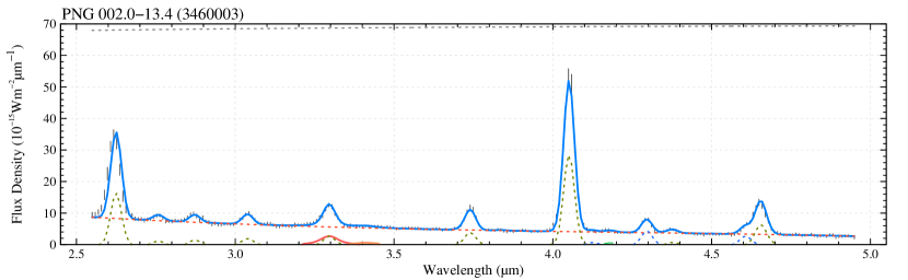
Figure 7: The AKARI/IRC 2.5–5.0$\,\mu$m spectra. Explanations of the lines are shown in the bottom of the figures.

Figure 7: Cont.—

Figure 7: Cont.—

Figure 7: Cont.—

Figure 7: Cont.—

Figure 7: Cont.—

Figure 7: Cont.—

Figure 7: Cont.—

Figure 7: Cont.—

Figure 7: Cont.—

Figure 7: Cont.—

Figure 7: Cont.—

Figure 7: Cont.—

Figure 7: Cont.—

Figure 7: Cont.—

Figure 7: Cont.—

Figure 7: Cont.—

Appendix A Uncertainty in $A_{V}$

There are several hydrogen recombination lines in the $2.5$–$5.0\,\mu$m spectrum. Extinction can be estimated based on the intensity ratio of these lines. The accuracy of the estimated extinction heavily depends on the signal-to-noise ratio (${\rm S/N}$) of the intensity ratio. This chapter describes the method to derive the extinction based on the IRC spectrum and shows that a typical uncertainty in ${\rm A}_{V}$ is ${\sim}1\,{\rm mag}$ for the PNSPC samples.

The observed intensity of the line emission $X$ is given by $I_{X}^{\rm obs}=I_{X}{\rm e}^{-\tau_{X}}$, where $I_{X}$ is the intrinsic intensity and $\tau_{X}$ is the extinction at the line $X$. The observed intensity ratio of the line $X$ to $Y$ is

$$\frac{I_{X}^{\rm obs}}{I_{Y}^{\rm obs}}=\frac{I_{X}}{I_{Y}}\exp\left(-\alpha(X,Y){\rm A}_{V}\right),$$ (A1)

where $\alpha(X,Y)$ is defined by $(\tau_{X}-\tau_{Y})/{{\rm A}_{V}}$, which is a constant value specific to the extinction curve. Thus, the extinction is estimated by

$${\rm A}_{V}=\frac{\log x_{\rm int}-\log x_{\rm obs}}{\alpha(X,Y)},$$ (A2)

where $x_{\rm int}$ is $I_{X}/I_{Y}$ and $x_{\rm obs}$ is $I_{X}^{\rm obs}/I_{Y}^{\rm obs}$. Given that the line $X$ and $Y$ are Brackett-$\alpha$ (Br$\alpha$) and $\beta$ (Br$\beta$), respectively, the intrinsic intensity ratio is about $0.57$ assuming the Case-B condition (Baker & Menzel, 1938) with the electron density of $10^{4}\,$K and the electron density of $10^{4}\,{\rm cm^{-3}}$. The ratio is less sensitive to either the electron temperature or density. We adopt the extinction curve given by Mathis (1990). The value of $\alpha({\rm Br}\beta,{\rm Br}\alpha)$ is about $0.041$. The extinction estimated from the Brackett-$\beta$ to $\alpha$ ratio is

$${\rm A}_{V}({\rm Br}\beta,{\rm Br}\alpha)\simeq{-}24.6\log x_{\rm obs}-13.7.$$ (A3)

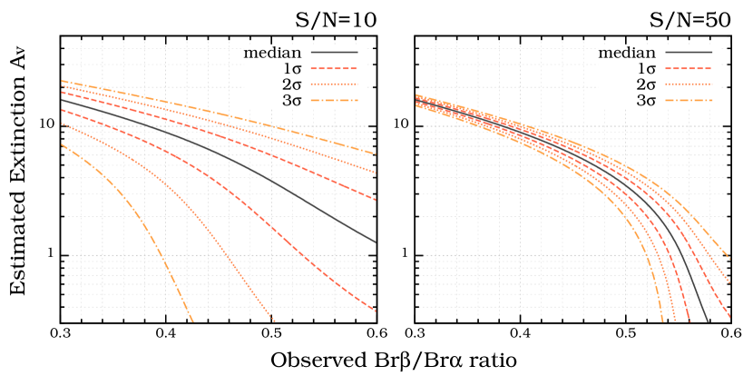
Figure 19: Estimated extinction and uncertainty. The dashed, dotted, and dot-dashed contours show the confidence intervals of the 1-, 2-, and 3-$\sigma$, respectively.

The uncertainty in ${\rm A}_{V}({\rm Br}\beta,{\rm Br}\alpha)$ is investigated. The measured intensity ratio ($x_{\rm obs}$) includes a statistical error. Define the error by $\sigma$. Assuming that the variation in $x_{\rm obs}$ is given by a normal distribution, the posterior probability distribution of the intensity ratio $(\bar{x}_{\rm obs})$ is given by

$${\rm prob}(\bar{x}_{\rm obs}|\,x_{\rm obs},\sigma)\propto\frac{1}{\sqrt{2\pi}\sigma}\exp\left(-\frac{(x_{\rm obs}-\bar{x}_{\rm obs})^{2}}{2\sigma^{2}}\right){\rm prob}(\bar{x}_{\rm obs}),$$ (A4)

where ${\rm prob}(\bar{x}_{\rm obs})$ is the prior distribution of $\bar{x}_{\rm obs}$ assumed to be a uniform distribution from $0$ to $x$. From Equations (A3) and (A4), the posterior distribution of ${\rm A}_{V}({\rm Br}\beta,{\rm Br}\alpha)$ is given by

$${\rm prob}({\rm A}_{V}|\,x_{\rm obs},\sigma)\propto{\rm prob}(\bar{x}_{\rm obs}|\,x_{\rm obs}){\rm prob}(\bar{x}_{\rm obs}).$$ (A5)

The results for ${\rm S/N}=10$ and $50$ are shown in Figure 19. The horizontal axis shows the observed intensity ratio ($x_{\rm obs}$), while the vertical axis is the estimated ${\rm A}_{V}$ value. The gray solid line indicates the median extinction ${\rm A}_{V}$. The red dashed, orange dotted, and yellow dot-dashed contours show the 1-, 2-, and 3-$\sigma$ confidence intervals, respectively. The typical ${\rm S/N}$ for the PNSPC spectrum is about $50$. Figure 19 suggests that the extinction estimated from the Br$\alpha$/Br$\beta$ ratio are quite uncertain when ${\rm A}_{V}\sim 1$–$3\,$mag. Figure 13 shows that the ${\rm A}_{V}$ values are typically less than about $2\,{\rm mag}$ for the PNSPC samples. Thus, it is practically impossible to precisely estimate the extinction of the PNSPC samples without using ancillary data such as the intensity of the H$\beta$ emission. The standard errors on ${\rm A}_{V}$ derived from the Br$\beta$/Br$\alpha$ and H$\beta$/Br$\alpha$ ratios are estimated to be about $0.5$ and $0.02\,$mag., respectively. The intrinsic line ratio may depend on the electron temperature and density. The impact is much larger for the H$\beta$/Br$\alpha$ ratio, but the variations in them can change ${\rm A}_{V}$ at most by $0.3\,$mag. Even though these variations are taken into account, the extinction derived from the H$\beta$/Br$\alpha$ ratio is much more reliable than that from the Br$\beta$/Br$\alpha$ ratio.

References

- Acker (1978) Acker, A. 1978, Astronomy and Astrophysics Supplement Series, 33, 367
- Acker et al. (1992) Acker, A., Marcout, J., Ochsenbein, F., Stenholm, B., & Tylenda, R. 1992, Strasbourg-ESO Catalogue of Galactic Planetary Nebulae, Parts I, II (Garching, Germany: European Southern Observatory)
- Allain et al. (1996a) Allain, T., Leach, S., & Sedlmayr, E. 1996a, Astronomy and Astrophysics, 305, 602
- Allain et al. (1996b) —. 1996b, Astronomy and Astrophysics, 305, 616
- Amnuel et al. (1984) Amnuel, P. R., Guseinov, O. K., Novruzova, K. I., & Rustamov, I. S. 1984, Astrophysics and Space Science, 107, 19
- Baker & Menzel (1938) Baker, J. G., & Menzel, D. H. 1938, The Astrophysical Journal, 88, 52
- Beintema et al. (1996) Beintema, D. A., van den Ancker, M. E., Molster, F. J., et al. 1996, Astronomy and Astrophysics, 315, L369
- Bernard-Salas et al. (2009) Bernard-Salas, J., Peeters, E., Sloan, G. C., et al. 2009, The Astrophysical Journal, 699, 1541
- Bernard-Salas et al. (2008) Bernard-Salas, J., Pottasch, S. R., Gutenkunst, S., Morris, P. W., & Houck, J. R. 2008, The Astrophysical Journal, 672, 274
- Bernard-Salas & Tielens (2005) Bernard-Salas, J., & Tielens, A. G. G. M. 2005, Astronomy and Astrophysics, 431, 523
- Blöcker (1995) Blöcker, T. 1995, Astronomy and Astrophysics, 299, 755
- Boulanger et al. (2011) Boulanger, F., Onaka, T., Pilleri, P., & Joblin, C. 2011, in EAS Publications Series, Vol. 46, PAHs and the Universe: A Symposium to Celebrate the 25th Anniversary of the PAH Hypothesis (Toulouse, France: EAS Publications Series), 399–405
- Cahn et al. (1992) Cahn, J. H., Kaler, J. B., & Stanghellini, L. 1992, Astronomy and Astrophysics Supplement Series, 94, 399
- Cohen et al. (1986) Cohen, M., Allamandola, L., Tielens, A. G. G. M., et al. 1986, The Astrophysical Journal, 302, 737
- Cohen & Barlow (2005) Cohen, M., & Barlow, M. J. 2005, Monthly Notices of the Royal Astronomical Society, 362, 1199
- Cutri et al. (2012) Cutri, R. M., Wright, E. L., Conrow, T., et al. 2012, VizieR Online Data Catalog, 2311
- Delgado-Inglada & Rodríguez (2014) Delgado-Inglada, G., & Rodríguez, M. 2014, The Astrophysical Journal, 784, 173
- Dobashi et al. (2005a) Dobashi, K., Uehara, H., Kandori, R., et al. 2005a, Publications of the Astronomical Society of Japan, 57, 1
- Dobashi et al. (2005b) —. 2005b, Publications of the Astronomical Society of Japan, 57, 417
- Draine & Li (2001) Draine, B. T., & Li, A. 2001, The Astrophysical Journal, 551, 807
- Dwek et al. (1997) Dwek, E., Arendt, R. G., Fixsen, D. J., et al. 1997, The Astrophysical Journal, 475, 565
- Gathier et al. (1986a) Gathier, R., Pottasch, S. R., & Goss, W. M. 1986a, Astronomy and Astrophysics, 157, 191
- Gathier et al. (1986b) Gathier, R., Pottasch, S. R., & Pel, J. W. 1986b, Astronomy and Astrophysics, 157, 171
- Guzman-Ramirez et al. (2014) Guzman-Ramirez, L., Lagadec, E., Jones, D., Zijlstra, A. A., & Gesicki, K. 2014, Monthly Notices of the Royal Astronomical Society, 441, 364
- Guzman-Ramirez et al. (2011) Guzman-Ramirez, L., Zijlstra, A. A., Níchuimín, R., et al. 2011, Monthly Notices of the Royal Astronomical Society, 414, 1667
- Harrington & Feibelman (1983) Harrington, J. P., & Feibelman, W. A. 1983, The Astrophysical Journal, 265, 258
- Joblin et al. (1996) Joblin, C., Tielens, A. G. G. M., Allamandola, L. J., & Geballe, T. R. 1996, The Astrophysical Journal, 458, 610
- Kaler (1976) Kaler, J. B. 1976, The Astrophysical Journal, 210, 843
- Kaler (1978) —. 1978, The Astrophysical Journal, 220, 887
- Kaler & Jacoby (1991) Kaler, J. B., & Jacoby, G. H. 1991, The Astrophysical Journal, 372, 215
- Lumsden et al. (2001) Lumsden, S. L., Puxley, P. J., & Hoare, M. G. 2001, Monthly Notices of the Royal Astronomical Society, 320, 83
- Maciel (1984) Maciel, W. J. 1984, Astronomy and Astrophysics Supplement Series, 55, 253
- Mathis (1990) Mathis, J. S. 1990, Annual Review of Astronomy and Astrophysics, 28, 37
- Mendez et al. (1988) Mendez, R. H., Kudritzki, R. P., Herrero, A., Husfeld, D., & Groth, H. G. 1988, Astronomy and Astrophysics, 190, 113
- Micelotta et al. (2010) Micelotta, E. R., Jones, A. P., & Tielens, A. G. G. M. 2010, Astronomy and Astrophysics, 510, 37
- Mori et al. (2012) Mori, T. I., Sakon, I., Onaka, T., et al. 2012, The Astrophysical Journal, 744, 68
- Noble et al. (2013) Noble, J. A., Fraser, H. J., Aikawa, Y., Pontoppidan, K. M., & Sakon, I. 2013, The Astrophysical Journal, 775, 85
- Ohsawa et al. (2012) Ohsawa, R., Onaka, T., Sakon, I., et al. 2012, The Astrophysical Journal Letters, 760, L34
- Onaka et al. (2007) Onaka, T., Matsuhara, H., Wada, T., et al. 2007, Publications of the Astronomical Society of Japan, 59, 401
- Phillips (2003) Phillips, J. P. 2003, Monthly Notices of the Royal Astronomical Society, 344, 501
- Phillips & Márquez-Lugo (2011) Phillips, J. P., & Márquez-Lugo, R. A. 2011, Revista Mexicana de Astronomia y Astrofisica, 47, 83
- Pottasch (1983) Pottasch, S. R. 1983, in IAU Symposium, Vol. 103, Planetary Nebulae (London, United Kingdom: Dordrecht, D. Reidel Publishing Co.), 391–409
- Pottasch & Bernard-Salas (2006) Pottasch, S. R., & Bernard-Salas, J. 2006, Astronomy and Astrophysics, 457, 189
- Pottasch et al. (1984) Pottasch, S. R., Baud, B., Beintema, D., et al. 1984, Astronomy and Astrophysics, 138, 10
- Preite-Martinez et al. (1989) Preite-Martinez, A., Acker, A., Köppen, J., & Stenholm, B. 1989, Astronomy and Astrophysics Supplement Series, 81, 309
- Preite-Martinez et al. (1991) —. 1991, Astronomy and Astrophysics Supplement Series, 88, 121
- Roche et al. (1996) Roche, P. F., Lucas, P. W., Hoare, M. G., Aitken, D. K., & Smith, C. H. 1996, Monthly Notices of the Royal Astronomical Society, 280, 924
- Sabbadin (1986) Sabbadin, F. 1986, Astronomy and Astrophysics Supplement Series, 64, 579
- Sakon et al. (2008) Sakon, I., Onaka, T., Wada, T., et al. 2008, in Society of Photo-Optical Instrumentation Engineers (SPIE) Conference Series, Vol. 7010, Space Telescopes and Instrumentation 2008: Optical, Infrared, and Millimeter, 88
- Schönberner (1983) Schönberner, D. 1983, The Astrophysical Journal, 272, 708
- Schönberner & Blöcker (1996) Schönberner, D., & Blöcker, T. 1996, Astrophysics and Space Science, 245, 201
- Schönberner et al. (2005) Schönberner, D., Jacob, R., Steffen, M., et al. 2005, Astronomy and Astrophysics, 431, 963
- Schutte et al. (1993) Schutte, W. A., Tielens, A. G. G. M., & Allamandola, L. J. 1993, The Astrophysical Journal, 415, 397
- Skrutskie et al. (2006) Skrutskie, M. F., Cutri, R. M., Stiening, R., et al. 2006, The Astronomical Journal, 131, 1163
- Sloan et al. (1997) Sloan, G. C., Bregman, J. D., Geballe, T. R., Allamandola, L. J., & Woodward, C. E. 1997, The Astrophysical Journal, 474, 735
- Sloan et al. (2003) Sloan, G. C., Kraemer, K. E., Price, S. D., & Shipman, R. F. 2003, The Astrophysical Journal Supplement Series, 147, 379
- Smith & McLean (2008) Smith, E. C. D., & McLean, I. S. 2008, Astrophysical Journal, 676, 408
- Stanghellini et al. (2012) Stanghellini, L., García-Hernández, D. A., García-Lario, P., et al. 2012, The Astrophysical Journal, 753, 172
- Stanghellini et al. (2007) Stanghellini, L., García-Lario, P., García-Hernández, D. A., et al. 2007, The Astrophysical Journal, 671, 1669
- Stanghellini & Haywood (2010) Stanghellini, L., & Haywood, M. 2010, The Astrophysical Journal, 714, 1096
- Storey & Hummer (1995) Storey, P. J., & Hummer, D. G. 1995, Monthly Notices of the Royal Astronomical Society, 272, 41
- Tokunaga et al. (1991) Tokunaga, A. T., Sellgren, K., Smith, R. G., et al. 1991, Astrophysical Journal, 380, 452
- Volk & Cohen (1990) Volk, K., & Cohen, M. 1990, The Astronomical Journal, 100, 485
- Wright et al. (2010) Wright, E. L., Eisenhardt, P. R. M., Mainzer, A. K., et al. 2010, The Astronomical Journal, 140, 1868