Statistics of the stochastically-forced Lorenz attractor by the Fokker-Planck equation and cumulant expansions

Abstract

We investigate the Fokker-Planck description of the equal-time statistics of the three-dimensional Lorenz-63 attractor with additive white noise. The invariant measure is found by computing the zero (or null) mode of the linear Fokker-Planck operator as a problem of sparse linear algebra. Two variants are studied: A self-adjoint construction of the linear operator, and the replacement of diffusion with hyperdiffusion. We also access the low-order statistics of the system by a perturbative expansion in equal-time cumulants. Comparison is made to statistics obtained by the standard approach of accumulation via direct numerical simulation. Theoretical and computational aspects of the Fokker-Planck and cumulant expansion methods are discussed.

I Introduction

Chaotic dynamical systems often have a well-defined statistical steady state. Traditionally statistics are estimated by their accumulation through Direct Numerical Simulation (DNS) starting from an ensemble of initial conditions. If the basin of attraction is ergodic, ensemble averaging can be replaced by time-averaging over a single long trajectory. Rare but large deviations may occur, however, necessitating extremely long integration times. An alternative and more efficient approach solves for the statistics directly. Depending on the question to be answered, such Direct Statistical Simulation (DSS) can focus on various statistical quantities such as the the probability distribution function (PDF) or invariant measure, the low-order equal-time moments, autocorrelations in time, or large deviations.

This paper presents two different types of DSS. The first, the Fokker-Planck equation (FPE), describes the flow of probability density in phase space, respecting the conservation of total probability. Consider a trajectory governed by the differential equation:

$$\frac{d\vec{x}}{dt}=\vec{V}(\vec{x})+\vec{\eta}(t)$$ (1)

where $\vec{\eta}(t)$ is additive stochastic forcing. The FPE for this system is:

$$\frac{\partial P(\vec{x},t)}{\partial t}=-\hat{L}_{FPE}P(\vec{x},t)$$ (2)

where we will call $\hat{L}_{FPE}$ the (linear) FPE operator. The placement of the negative sign in front of the operator $\hat{L}_{FPE}$ in Eq. 2 is for convenience: The operator $\hat{L}_{FPE}$ is then semipositive definite, and the steady-state statistics are determined by the ground state. In the special case where $\vec{\eta}$ is Gaussian additive white noise with no mean and covariance given by

$$\langle\eta_{i}(t)~{}\eta_{j}(t^{\prime})\rangle=2\Gamma_{ij}~{}\delta(t-t^{\prime}),$$ (3)

with angular brackets $\langle\ldots\rangle$ indicating a short time-average, only a finite number of terms appear in the FPE operator pawula1967approximation :

$$\hat{L}_{FPE}P=\vec{\nabla}\cdot(\vec{V}P)-\Gamma\nabla^{2}P.$$ (4)

Additive stochastic forcing smears out the PDF $P$ through diffusion in phase space. A canonical example is the one-dimensional Ornstein-Uhlenbeck process with trajectories governed by

$$\dot{x}=-ax+\eta(t).$$ (5)

The corresponding FPE is

$$\frac{\partial P(x,t)}{\partial t}=\frac{\partial}{\partial x}[axP(x,t)]+\Gamma\frac{\partial^{2}P(x,t)}{\partial x^{2}}$$ (6)

that has a steady-state solution that is readily found to be Gaussian:

$$P(x)=\sqrt{\frac{a}{2\pi\Gamma}}~{}e^{-ax^{2}/2\Gamma}\ .$$ (7)

As we will see, stochastic forcing also needs to be introduced to regulate strange attractors at small scales. As the fractal structure of a strange attractor cannot be resolved on a lattice, it is necessary to smooth the structure at the lattice length scale. We use additive stochastic forcing for this purpose.

Direct solution of the FPE is most commonly carried out for one dimensional systems. Extension to higher dimensions is conceptually straightforward, but numerically challenging pichler2013numerical . The objective of the present paper is to apply the FPE to a three dimensional chaotic system. Numerical solutions have been developed based on finite elements bergman1992robust ; von2000calculation , finite differences kumar2006 , and path integrals naess1994response . Here we depart from these traditional methods by instead directly solving for the zero or null mode of a finite-difference discretized FPE operator, thus obviating the time-consuming and costly steps of computing the transient probability distributions. We illustrate this new method by applying it to the Lorenz-63 system lorenz1963deterministic with additive stochastic forcing. Although a phenomenological FPE has been applied for a quantum system without the addition of stochastic forcing PhysRevLett.110.050401 , we follow previous work thuburn2005climate ; gradivsek2000analysis ; agarwal2016maximal ; PhysRevE.92.062922 ; Kumar20142040 and add small additive white noise to wash out fractal structure below the lattice scale.

Since numerical solution of the FPE in larger numbers of dimensions is stymied by the “curse of dimensionality” it is important to develop alternative forms of DSS. Accordingly we also explore a second type of DSS, an expansion in equal-time cumulants that can be applied to high-dimensional dynamical systems. A cumulant expansion was employed for the Orszag-McLaughlin attractor in Ref. ma2005exact . For the Lorenz attractor we show that low-order statistics are well reproduced at third order truncation.

The paper is organized as follows. Section II briefly describes the Lorenz-63 system with additive stochastic forcing, and its numerical integration. Two different sets of parameters are considered, both of which yield chaotic behavior. Section III describes the FPE and the numerical method that we use to find the invariant measure. Equal-time statistics so obtained are compared to those found through accumulation by DNS. We study the scaling of the spectral gap of the linear FPE operator as the stochastic forcing is varied. Two extensions to the method are also considered: A self-adjoint construction of the linear operator, and the replacement of diffusion with hyperdiffusion. Section IV presents the cumulant expansion technique and its evaluation by comparison to DNS. Some conclusions are presented in Section V.

II Lorenz-63 Attractor With Additive Stochastic Forcing

The Lorenz-63 attractor is a three dimensional, chaotic system that was originally derived by applying a severe Galerkin approximation to the equations of motion (EOMs) for Rayleigh-Bénard convection with stress-free boundary conditions lorenz1963deterministic . We study an extension with additive stochastic forcing thuburn2005climate ; gradivsek2000analysis ; agarwal2016maximal ; PhysRevE.92.062922 ; Kumar20142040 that obeys Eq. 3. Such additive white noise can model fast or unresolved physical processes that are not explicitly described.

$$\dot{x} = \sigma(y-x)+\eta_{1}(t)$$

$$\dot{y} = x(\rho-z)-y+\eta_{2}(t)$$

$$\dot{z} = xy-\beta z+\eta_{3}(t)$$ (8)

In this context $x$ is proportional to convective intensity, $y$ to the difference in temperature between ascending and descending currents, and $z$ to the vertical temperature profile’s deviation from linearity. Parameters $\beta$, $\rho$, and $\sigma$ are a geometric factor, the Rayleigh number, and the Prandtl number respectively. We also choose the covariance of the Gaussian white noise to be diagonal and isotropic: $\Gamma_{ij}=\Gamma~{}\delta_{ij}$.

We study the strange attractor at two different sets of parameters. The conventional (classic) parameters are $\beta=1.0$, $\rho=26.5$, and $\sigma=3.0$. We also examine the case with the geometric factor changed to $\beta=0.16$. This modification enhances layering in the PDF. Since the geometric factor is related to the size of the attractor, a reduction in $\beta$ shrinks the attractor which in turn allows for a reduction in the stochastic forcing whilst keeping the structure sufficiently smooth at the lattice length scale. Each attractor has a slow time scale corresponding to transitions between the wings of the butterfly, and a fast time scale for orbits about each wing. The fast time-scale is $\tau\simeq 1$.

II.1 Direct Numerical Simulation

The Eq. 8 EOMs are integrated forward in time with the fourth-order accurate Runge-Kutta algorithm with fixed time step $\delta t=0.01$. Stochastic forcing, drawn from a normal distribution, is updated at intervals of $\Delta t=0.1$ and interpolated at intermediate times $\delta t$. Note that there is a good separation of time scales with $\tau\gg\Delta t\gg\delta t$ following the reasoning of Ref. lilly1969numerical .

Statistics are accumulated up to a final time $T=2\times 10^{7}$. The PDF is estimated from the histogram that results from binning the trajectory into cubic boxes. The PDF is projected onto a plane by integrating over the direction perpendicular to the plane; for instance:

$$P(x,y)=\int_{-\infty}^{\infty}P(x,y,z)~{}dz\ .$$ (9)

Figures 1, 3 and 5 show that even small stochastic forcing smoothes out the fine structure of the strange attractor Heninger2016 ; in particular the ring-like steps in the PDF disappear.

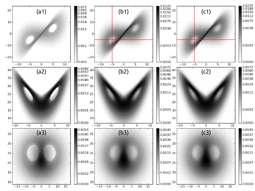
Figure 1: (Color online) (a) PDF of the unforced Lorenz system (binned on a $637^{3}$ grid) accumulated by DNS. Classic Lorenz parameters are used (see Sec. II). (b) Same, but for the stochastically forced $(\Gamma=0.2)$ ($478^{3}$ grid). Note that the fine rings visible in the unforced system are washed out by the noise. (c) PDF of the stochastically forced attractor ($\Gamma=0.2$) as obtained from the zero-mode of $\hat{L}_{FPE}$ on a $160^{3}$ grid and for $x\in[-12.5,~{}12.5]$, $y\in[-24,~{}24]$ and $z\in[1,~{}45]$. The JDQR algorithm is employed. Rows (1), (2) and (3) correspond to the $x-y$, $x-z$ and $y-z$ projections of the PDF respectively. Good agreement between (b) DNS and (c) FPE is evident. Red lines correspond to the cross-sections shown in Figure 2.

III Fokker-Planck Equation

The FPE is an attractive alternative to the accumulation of statistics by DNS. The linear FPE operator for the Lorenz system,

$$\hat{L}_{FPE}P=\vec{\nabla}\cdot[(\sigma(y-x),~{}x(\rho-z)-y,~{}xy-\beta z)P]-\Gamma\nabla^{2}P$$ (10)

is positive-definite in the sense that the real part of the eigenvalues are non-negative (if that were not the case, Eq. 2 would diverge). The equal-time PDF of the FPE is the zero or null mode of $\hat{L}_{FPE}$. By discretizing the operator on a lattice, the problem of finding the zero mode is converted as a problem of sparse linear algebra.

III.1 Numerical Solution

A standard center-difference scheme is used to discretize the derivatives that appear in Eq. 10:

$$f_{i}^{\prime} \approx \frac{f_{i+1}-f_{i-1}}{2\Delta x}$$

$$f_{i}^{\prime\prime} \approx \frac{f_{i+1}-2f_{i}+f_{i-1}}{\Delta x^{2}}\ .$$ (11)

The PDF of the unforced Lorenz attractor has compact support but once stochastic forcing is included the PDF is non-zero but exponentially small throughout phase space. In the numerical calculation, the probability density $P$ is taken to vanish outside of the domain. The zero-mode of $\hat{L}_{FPE}$ is found with the use of a preconditioned Jacobi-Davidson QR (JDQR) algorithm sleijpen2000jacobi ; fokkema1998jacobi that computes the partial Schur decomposition of a matrix with error tolerance set to $10^{-5}$. We have checked that our results do not change appreciably for tighter tolerances. Although the JDQR algorithm is well-suited for sparse matrices, requiring only the action of a matrix multiplying a vector, we were unable to find a suitable sparse preconditioner. A sparse preconditioner would enable a substantial increase in resolution. The Jacobi correction equation is preconditioned following section 3.2 of Ref. fokkema1998jacobi and solved using the generalized minimal residual (GMRES) method using Matlab. The highest resolution we have been able to reach is $160^{3}$ with 500 GB of memory. To the best of our knowledge this is the largest number of grid points for which the Fokker-Planck equation has been simulated (for comparison, more than double the number reached by Kumar and Narayanan (2016) kumar2006 ). This is made possible by re-expressing the time-dependant Fokker-Planck problem to a sparse linear algebra problem. On the $160^{3}$ grid the $\hat{L}_{FPE}$ matrix has $28,518,400$ non-zero elements and a sparsity of $1.70\times 10^{-6}$.

Modes at the maximal wavenumber decay diffusively due to the stochastic forcing with a decay timescale $\tau_{d}$ given by

$$\tau_{d}^{-1}=\frac{\pi^{2}\Gamma}{4}[(\Delta x)^{-2}+(\Delta y)^{-2}+(\Delta z)^{-2}]$$ (12)

Equating this time scale to the timescale of fast dynamics $\tau$ provides an estimate of the effective resolution of the discretized FPE.

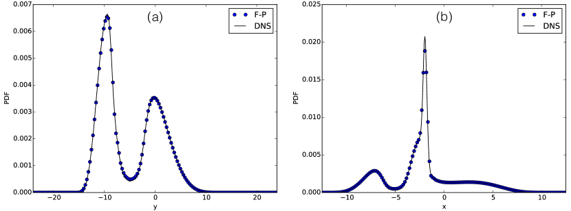
Figure 2: (a) Vertical and (b) horizontal slices along the red lines of the $x-y$ planar projection shown in Fig. 1. The DNS and FPE methods agree quantitatively.

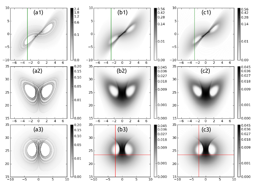
Figure 3: (Color online) (a) PDF of the unforced Lorenz system (binned on a $637^{3}$ grid) accumulated by DNS. Modified parameters are used (see Sec. II). (b) Same, but for the stochastically forced $(\Gamma=0.02)$ ($478^{3}$ grid). Note that the fine rings visible in the unforced system are washed out by the noise. (c) PDF of the stochastically forced attractor ($\Gamma=0.02$) as obtained from the zero-mode of $\hat{L}_{FPE}$ on a $160^{3}$ grid and for $x\in[-7,~{}7]$, $y\in[-10,~{}10]$ and $z\in[15,~{}35]$. Rows (1), (2) and (3) correspond to the $x-y$, $x-z$ and $y-z$ projections of the PDF respectively. Good agreement between (b) DNS and (c) FPE is evident. Red lines correspond to the cross-sections shown in Figure 4 and green lines correspond to the cross-section shown in Figure 5

.

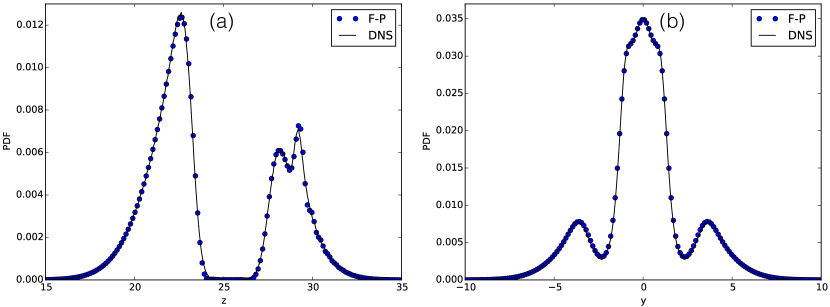
Figure 4: (a) Vertical and (b) horizontal slices along the red lines of the $y-z$ planar projection shown in Fig. 3. The DNS and FPE methods agree quantitatively.

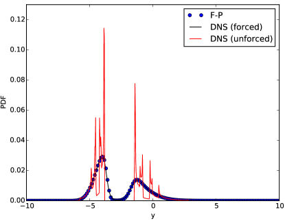
Figure 5: (Color online) Cross-section through the $x-y$ planar projection of the PDF where $x=-2.77$ for unforced DNS, stochastically forced DNS, and stochastically forced FPE (with $\Gamma=0.02$). Modified parameters are used. Sharp peaks in probability seen in the unforced Lorenz system are eliminated by the stochastic forcing.

Figures 1, 2, 3, 4 and 5 show good quantitative agreement between PDFs accumulated by DNS and those obtained from the zero mode of the FPE operator. Fine structure evident in the $x-z$ and $y-z$ projections of the PDF for the Lorenz attractor with modified parameters, Figure 3, is reproduced by the FPE. The modified parameters also demonstrate the sensitivity of the fractal structure to stochastic forcing. Even forcing as small as $\Gamma=0.02$ washes out the ring-like steps in the PDF in Figure 3, also shown by the selected horizonal slice in Figure 5.

III.2 Eigenvalue Spectra of the Fokker-Planck Operator

The gap to the eigenmode with the smallest non-zero real part of its eigenvalue is of interest as it corresponds to the slowest relaxation rate in the statistics towards the statistical steady state. Likewise the imaginary components of the eigenvalues of the linear FPE operator set the quasi-periodic frequency of the dynamical system (see Section II for a discussion of the slow and fast time scales). This interpretation of the real and imaginary components of the eigenvalues can be illustrated analytically with a two-dimensional linear Ornstein-Uhlenbeck system with circular orbits of period $2\pi$ that decay at rate $\alpha$:

$$\dot{x} = y-\alpha x+\eta_{1}(t)$$

$$\dot{y} = -x-\alpha y+\eta_{2}(t).$$ (13)

The eigenvalues of the FPE operator of this system are $\lambda_{n,m}=\alpha n\pm im$ where $m,~{}n$ are non-negative integers that are either both odd, or both even, and $m\leq n$. (The eigenvalues can be found by transforming to polar coordinates and expressing the PDF as a separable solution $P(r,~{}\theta)=R(r)~{}\Theta(\theta)$ with the radial equation solved using generalized Laguerre polynomials.) Because the system of Eq. 13 is linear, the stochastic forcing does not affect the spectra. The real parts of the eigenvalues are determined by the decay rate $\alpha$ whereas the imaginary part is set by the orbital period.

The spectrum of low-lying eigenvalues is shown in Figure 6 with the complex eigenvalues appearing in conjugate pairs because $\hat{L}_{FPE}$ is purely real-valued. Increased stochastic forcing increases the values of the real components of the eigenvalues of the FPE operator, in turn shortening the relaxation timescale. Linear extrapolation to the unforced $(\Gamma=0)$ limit yields a real eigenvalue of $0.0802$ corresponding to a relaxation timescale of about $12$ in accord with expectations.

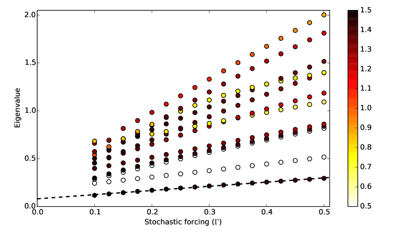
Figure 6: (Color online) Real component of the first 12 non-zero eigenvalues of the linear FPE operator of the Lorenz system (on an $80^{3}$ lattice grid) as a function of stochastic forcing $(\Gamma)$. Modified parameters are used (see Sec. II) with $x\in[-12.5,~{}12.5]$, $y\in[-17.5,~{}17.5]$ and $z\in[7.5,~{}42.5]$. The phase of each eigenvalue is represented by the color of the points with white correspond to a phase of zero. A linear extrapolation of the first non-zero eigenvalue to $\Gamma=0$ is shown. The second and third non-zero eigenvalues are purely real.

Likewise the non-zero imaginary parts of the eigenvalues in Fig. 6 correspond to the oscillation frequency around each of the two wings of the Lorenz attractor as well as the slower rate of transitions between the two wings.

III.3 Extensions

We consider two modifications to the FPE operator. Self-adjoint constructions of the linear operator are considered first, and then the replacement of diffusion with hyperdiffusion.

III.3.1 Self-Adjoint Linear FPE Operators:

We investigate whether or not self-adjoint generalizations of the linear FPE operator have any advantages. One way to construct such an operator is to double the size of the linear space by introducing the operator

$$\hat{H}_{2}=\left(\begin{array}[]{cc}0&\hat{L}_{FPE}\\ \hat{L}_{FPE}^{\dagger}&0\end{array}\right)\$$ (14)

that by construction obeys $\hat{H}_{2}^{\dagger}=\hat{H}_{2}$. $\hat{H}_{2}$ is no longer positive-definite; instead its eigenvalue spectrum is symmetric about 0. Finding the zero mode therefore requires a numerical algorithm that can target the middle of the spectrum. Alternatively the operator

$$\hat{H}_{1}\equiv\hat{L}_{FPE}^{\dagger}~{}\hat{L}_{FPE}$$ (15)

is self-adjoint, positive-definite, and has the same ground state as $\hat{L}_{FPE}$. To see this define $|V\rangle\equiv\hat{L}_{FPE}|\Psi_{0}\rangle$ where $|\Psi_{0}\rangle$ is the zero mode of $\hat{H}_{1}$. Then $\langle\Psi_{0}|\hat{L}_{FPE}^{\dagger}\hat{L}_{FPE}|\Psi_{0}\rangle=\langle V|V\rangle=0$ that implies that $|V\rangle$ must have zero norm, $|V\rangle=|0\rangle$, and $|\Psi_{0}\rangle$ is the zero mode of $\hat{L}_{FPE}$. The ground state of a quantum system has (under rather general conditions) no nodes so $\Psi_{0}(\vec{x})$ automatically produces a non-negative PDF – an added virtue of viewing steady-state solutions of the FPE as a problem of linear algebra.

Because the ground state of $\hat{H}_{1}$ might possibly be found using simulated annealing or quantum annealing / adiabatic quantum computation finnila1994quantum ; santoro2006optimization , it is of interest to investigate its numerical solution. A drawback of $\hat{H}_{1}$ is that the eigenvalues are clustered more tightly around $0$ than those of $\hat{L}$, slowing convergence. We find that the ground state, computed using the Davidson algorithm davidson1975iterative ; davidson1993monster , matches that obtained from $\hat{L}_{FPE}$ alone.

III.3.2 Hyperdiffusion:

Another interesting variant to investigate is to replace diffusion in Eq. 10 with biharmonic hyperdiffusion:

$$-\Gamma\nabla^{2}\rightarrow\Gamma_{2}\nabla^{4}$$ (16)

As hyperdiffusion is more scale selective than ordinary diffusion, it acts to smooth out structure at the lattice scale while leaving larger structures intact. Holding the dissipation rate at the lattice scale fixed, $\Gamma_{2}$ scales inversely with the 4th power of the spacing (contrast with Eq. 12). Unlike ordinary diffusion that has a physical origin in stochastic forcing, hyperdiffusion violates realizability leading to negative probability densities (see for example section 4.3 of Ref. risken1996fokker ). Also hyperdiffusion reduces the sparseness of the discretized linear FPE operator, slowing computation. On an $80^{3}$ grid the PDF shows less fine structure as expected.

IV Cumulant Expansion

Numerical solution of the FPE for dynamical systems of dimension greater than 3 is increasingly difficult. Therefore it is of interest to explore other approaches to DSS. Here we use an expansion in low-order equal-time cumulants to find statistics of the Lorenz attractor. In addition to the Orszag-McLaughlin attractor ma2005exact , it has also been applied to a number of high-dimensional problems in fluids using spatial averaging marstonetal2008 ; tobiasdagonetal2011 ; tobiasmarston2013 ; parkerkrommes2013a ; parkerkrommes2014 ; squirebhattacharjee2014 ; marston2014direct ; aitchaalalmarstonetal2016 although sometimes ensemble averages are employed Bakas:2013bo ; Bakas:2015iy .

The EOMs for equal-time cumulants can be elegantly derived using the Hopf functional formalism frisch1995 ; tobiasdagonetal2011 . However it is also possible to derive them directly from the EOMs of the dynamical system. Consider a general system with quadratic nonlinearities:

$$\dot{q}_{i}=F_{i}+L_{ij}~{}q_{j}+Q_{ijk}~{}q_{j}q_{k}+\eta_{i}.$$ (17)

A Reynolds decomposition,

$$q_{i}=\overline{q_{i}}+q_{i}^{\prime}\ ,$$ (18)

of the dynamical variables $q_{i}$ into a mean and a fluctuation is the starting point. Here (and as discussed below) the average is chosen to be a mean over initial conditions drawn from a Gaussian distribution. The Reynolds decomposition obeys the rules:

$$\overline{\overline{q}_{i}} = \overline{q}_{i}$$

$$\overline{q^{\prime}_{i}} = 0$$

$$\overline{\overline{q}_{i}~{}q_{j}} = \overline{q}_{i}~{}\overline{q}_{j}.$$ (19)

The first cumulant, $c_{i}$, is the mean of $q_{i}$ and the second and third cumulants are given by centered moments of the fluctuations. By contrast the fourth cumulant is not a centered moment:

$$c_{i} \equiv \overline{q_{i}}$$

$$c_{ij} \equiv \overline{q_{i}^{\prime}q_{j}^{\prime}}$$

$$c_{ijk} \equiv \overline{q_{i}^{\prime}q_{j}^{\prime}q_{k}^{\prime}}$$

$$c_{ijk\ell} \equiv \overline{q_{i}^{\prime}q_{j}^{\prime}q_{k}^{\prime}q_{\ell}^{\prime}}-c_{ij}~{}c_{k\ell}-c_{ik}~{}c_{j\ell}-c_{i\ell}~{}c_{jk}\ .$$ (20)

These definitions ensure that the third and higher cumulants of a Gaussian distribution vanish.

The EOMs for the cumulants may be found directly. The equation of motion for the first cumulant is obtained by ensemble averaging Eq. 17 and using the definitions of the first and second cumulants in Eq. 20,

$$\frac{dc_{i}}{dt} = \overline{\frac{dq_{i}}{dt}}$$ (21)

$$= F_{i}+L_{ij}~{}\overline{q_{j}}+Q_{ijk}~{}\overline{q_{j}q_{k}}$$

$$= F_{i}+L_{ij}~{}c_{j}+Q_{ijk}~{}(c_{j}c_{k}+c_{jk}).$$

The tendency of the first cumulant involves the second cumulant. Truncating at first order by discarding the second cumulant, the CE1 approximation, shows that the first cumulant obeys the same EOMs as Eq. 17; hence there is no non-trivial fixed point solution. In general for quadratically nonlinear systems the tendency of the $(n)$-th cumulant requires knowledge of the $(n+1)$-th cumulant, the well-known closure problem. Thus the EOM for the second cumulants requires the first, second and third cumulants:

$$\frac{dc_{ij}}{dt} = 2\left\{\overline{\frac{dq_{i}^{\prime}}{dt}~{}q_{j}^{\prime}}\right\}$$ (22)

$$= 2\left\{\overline{\left(\frac{dq_{i}}{dt}-\frac{d\overline{q_{i}}}{dt}\right)q_{j}^{\prime}}\right\}$$

$$= 2\left\{\overline{\frac{dq_{i}}{dt}q_{j}^{\prime}}\right\}$$

$$= 2\left\{\overline{L_{ik}~{}q_{k}q_{j}^{\prime}+Q_{ik\ell}~{}q_{k}q_{\ell}q_{j}^{\prime}}\right\}+2\Gamma_{ij}$$

$$= \left\{2L_{ik}~{}c_{kj}+Q_{ik\ell}~{}(4c_{k}c_{\ell j}+2c_{k\ell j})\right\}+2\Gamma_{ij}\ .$$

The covariance matrix $\Gamma_{ij}$ of the stochastic forcing appears in the last two lines as (implicitly) a short-time averaging has been carried out in addition to ensemble averaging. The symmetrization operation $\left\{\ldots\right\}$ over all permutations of the free indices has been introduced for conciseness. In the case of a $2$-index variable such as the second cumulant it is defined as $\left\{c_{ij}\right\}=\frac{1}{2}(c_{ij}+c_{ji})$ and similarly for higher cumulants.

Because each higher cumulant carries an additional dimension with it, closure should be performed as soon as possible. Closing the EOMs at second order by discarding the contribution of the third cumulant $c_{ijk}$ (CE2) is sometimes possible marstonetal2008 and yields a realizable approximation (because the PDF is Gaussian that is non-negative everywhere). The CE2 EOMs can then be integrated forward in time by specifying as an initial condition non-zero first and second cumulants, corresponding to a normally distributed initial ensemble. However the Lorenz attractor is so nonlinear that the CE2 EOMs, integrated forward in time, do not reach a fixed point that would characterize a statistical steady state. Therefore we proceed to next order, CE3, by setting the fourth cumulant to zero, $c_{ijkl}=0$. The fourth centered moment may then be expressed in terms of the second and third cumulants:

$$\overline{q_{m}^{\prime}q_{n}^{\prime}q_{j}^{\prime}q_{k}^{\prime}} = c_{mn}c_{jk}+c_{mj}c_{nk}+c_{mk}c_{jn}+c_{mnjk}$$ (23)

$$\simeq c_{mn}c_{jk}+c_{mj}c_{nk}+c_{mk}c_{jn}\ \ \ {\rm(CE3)}$$

and the EOM for the third cumulant now closes:

$$\frac{dc_{ijk}}{dt} = 3\left\{\overline{\frac{dq_{i}^{\prime}}{dt}q_{j}^{\prime}q_{k}^{\prime}}\right\}$$ (24)

$$= 3\left\{\overline{\left(\frac{dq_{i}}{dt}-\frac{d\overline{q_{i}}}{dt}\right)q_{j}^{\prime}q_{k}^{\prime}}\right\}$$

$$= 3\left\{\overline{\frac{dq_{i}}{dt}q_{j}^{\prime}q_{k}^{\prime}}-\frac{dc_{i}}{dt}\overline{q_{j}^{\prime}q_{k}^{\prime}}\right\}$$

$$= 3\left\{L_{im}~{}c_{mjk}+Q_{imn}~{}\left(2c_{m}c_{njk}-c_{mn}c_{jk}+\overline{q_{m}^{\prime}q_{n}^{\prime}q_{j}^{\prime}q_{k}^{\prime}}\right)\right\}$$

$$= \left\{3L_{im}~{}c_{mjk}+6Q_{imn}~{}\left(c_{m}c_{njk}+c_{mj}c_{nk}\right)\right\}-\frac{c_{ijk}}{\tau_{d}}.$$

In the final line of Eq. 24 a phenomenological eddy damping time scale, $\tau_{d}$, has been introduced to model the neglect of the fourth cumulant orszag1974lectures ; marston2014direct . CE2 is recovered in the limit $\tau_{d}\rightarrow 0$ as the third cumulant is suppressed in this limit. As $\tau_{d}$ is increased, contributions from the interactions of two fluctuations that produce another fluctuation begin to be felt. These nonlinear fluctuation + fluctuation $\rightarrow$ fluctuation interactions are dropped at order CE2, which retains only the fluctuation + fluctuation $\rightarrow$ mean and fluctuation + mean $\rightarrow$ fluctuation interactions marston2014direct . This can be seen be examining Eqs. 21 and 22 and observing that the second cumulant only interacts through $Q_{ijk}$ with the first cumulant, and not with itself. Upon increasing $\tau_{d}$ further eventually realizability is lost as the second cumulant develops negative eigenvalues that are unphysical kraichnan1980realizability ; hanggi1980remark ; marston2014direct . Furthermore the appearance of a negative eigenvalue triggers an instability and the time-integrated EOMs diverge. We note that non-zero third cumulants are a mark of a non-Gaussian PDF for which all higher cumulants would generically be non-zero as well. Therefore it is inconsistent to discard the fourth and higher cumulants, and that inconsistency makes itself felt in non-realizability.

An appealing feature of cumulant expansions is that they respect the symmetries of the dynamical system. For instance, the CE3 fixed point exactly respects $\overline{x}=\overline{y}=0$ due to the invariance of the Lorenz system under the reflection $\{x,y,z\}\rightarrow\{-x,-y,z\}$. This statistical symmetry is only approximately obeyed by DNS statistics accumulated over a finite time. Table LABEL:UnforcedCumulants compares the first and second cumulants of the unforced Lorenz attractor as accumulated by DNS to those obtained from CE3 for two different choices of the time scale $\tau_{d}$. Good qualitative agreement is found for both $\tau_{d}=0.1$ and $\tau_{d}=0.5$ demonstrating an insensitivity to the precise choice of the time scale. Table LABEL:ForcedCumulants displays the same cumulants, but now for the stochastically forced attractor. In addition statistics obtained from the FPE zero mode are shown, calculated as the PDF-weighted sums of the desired variable over the domain of the lattice. Though the small stochastic forcing has a large effect on the fine structure of the PDF, it only changes the covariances slightly.

Table 1: Comparison of the low-order statistically steady state cumulants of the unforced Lorenz attractor ($\Gamma=0$) as accumulated by DNS and as calculated with CE3. Modified Lorenz parameters are used (see Sec. II). Entries such as ${\cal O}(10^{-4})$ indicate that these mean values are tending to zero as time-averaging of DNS extends over increasing intervals of time.

Cumulant	DNS	CE3 $(\tau_{d}=0.1)$	CE3 $(\tau_{d}=0.5)$
$\overline{x}$	${\cal O}(10^{-4})$	0	0
$\overline{y}$	${\cal O}(10^{-4})$	0	0
$\overline{z}$	24.796	25.188	25.000
$\overline{x^{\prime}x^{\prime}}$	3.966	4.030	4.000
$\overline{x^{\prime}y^{\prime}}$	3.966	4.030	4.000
$\overline{x^{\prime}z^{\prime}}$	${\cal O}(10^{-5})$	0	0
$\overline{y^{\prime}y^{\prime}}$	5.395	4.392	4.908
$\overline{y^{\prime}z^{\prime}}$	${\cal O}(10^{-5})$	0	0
$\overline{z^{\prime}z^{\prime}}$	8.513	5.592	6.825

Table 2: As in Table LABEL:UnforcedCumulants but with added stochastic forcing ($\Gamma=0.02$).

Cumulant	DNS	FPE	CE3 $(\tau_{d}=0.1)$	CE3 $(\tau_{d}=0.5)$
$\overline{x}$	${\cal O}(10^{-5})$	${\cal O}(10^{-9})$	0	0
$\overline{y}$	${\cal O}(10^{-5})$	${\cal O}(10^{-9})$	0	0
$\overline{z}$	24.834	24.834	25.192	25.004
$\overline{x^{\prime}x^{\prime}}$	3.977	3.978	4.034	4.004
$\overline{x^{\prime}y^{\prime}}$	3.971	3.972	4.031	4.001
$\overline{x^{\prime}z^{\prime}}$	${\cal O}(10^{-5})$	${\cal O}(10^{-8})$	0	0
$\overline{y^{\prime}y^{\prime}}$	5.350	5.349	4.396	4.912
$\overline{y^{\prime}z^{\prime}}$	${\cal O}(10^{-4})$	${\cal O}(10^{-8})$	0	0
$\overline{z^{\prime}z^{\prime}}$	8.150	8.135	5.610	6.829

V Conclusion

Direct Statistical Simulation (DSS) is an attractive alternative to the accumulation of statistics by Direct Numerical Simulation (DNS). Transforming the problem of finding the equal-time statistics of dynamical systems into a problem of sparse linear algebra offers an accurate and elegant alternative to traditional approaches. It would be interesting to employ a sparse preconditioner for the large non-symmetric FPE operator studied here as this should permit even higher resolutions to be reached, possibly revealing the fine ring-like steps in the Lorenz attractor PDF. Galerkin discretizations of the linear operator may also be interesting to explore.

We also show that an expansion in equal-time cumulants through third order (CE3) is able to reproduce the low-order statistics of the attractor, despite its highly nonlinear nature. The cumulant expansion technique is especially good for higher dimensional systems due to its speed. Deterministic chaos and stochastic noise are seen to have similar effects on the low-order statistics knobloch1979statistical ; agarwal2016maximal with both contributing to the variance. By contrast Figure 5 shows that the deterministic dynamics of the strange attractor produces high-order statistics that stochastic forcing erases.

VI Acknowledgments

We are grateful to P. Zucker and D. Venturi for useful discussions. This research was supported in part by NSF DMR-1306806 and NSF CCF-1048701.

References

- [1] Hannes Risken. The Fokker-Planck equation: methods of solution and applications. Springer, 1984.
- [2] R.F. Pawula. Approximation of the linear Boltzmann equation by the Fokker-Planck equation. Physical Review, 162(1):186, 1967.
- [3] L Pichler, A Masud, and L.A. Bergman. Numerical Solution of the Fokker-Planck Equation by Finite Difference and Finite Element Methods - A Comparative Study. In Computational Methods in Stochastic Dynamics, pages 69–85. Springer, 2013.
- [4] L.A. Bergman and B.F. Spencer Jr. Robust numerical solution of the transient Fokker-Planck equation for nonlinear dynamical systems. In Nonlinear Stochastic Mechanics, pages 49–60. Springer, 1992.
- [5] Utz von Wagner and Walter V Wedig. On the calculation of stationary solutions of multi-dimensional Fokker–Planck equations by orthogonal functions. Nonlinear Dynamics, 21(3):289–306, 2000.
- [6] Pankaj Kumar and S. Narayanan. Solution of Fokker-Planck equation by finite element and finite difference methods for nonlinear systems. Sadhana, 31(4):445–461, 2006.
- [7] A Naess and B.K. Hegstad. Response statistics of van der Pol oscillators excited by white noise. Nonlinear Dynamics, 5(3):287–297, 1994.
- [8] Edward N Lorenz. Deterministic nonperiodic flow. Journal of the Atmospheric Sciences, 20(2):130–141, 1963.
- [9] Igor Tikhonenkov, Amichay Vardi, James R. Anglin, and Doron Cohen. Minimal Fokker-Planck Theory for the Thermalization of Mesoscopic Subsystems. Phys. Rev. Lett., 110:050401, Jan 2013.
- [10] J Thuburn. Climate sensitivities via a Fokker–Planck adjoint approach. Quarterly Journal of the Royal Meteorological Society, 131(605):73–92, 2005.
- [11] Janez Gradišek, Silke Siegert, Rudolf Friedrich, and Igor Grabec. Analysis of time series from stochastic processes. Physical Review E, 62(3):3146, 2000.
- [12] Sahil Agarwal and J.S. Wettlaufer. Maximal stochastic transport in the Lorenz equations. Physics Letters A, 380(1):142–146, 2016.
- [13] Jeffrey M. Heninger, Domenico Lippolis, and Predrag Cvitanović. Neighborhoods of periodic orbits and the stationary distribution of a noisy chaotic system. Phys. Rev. E, 92:062922, Dec 2015.
- [14] P. Kumar, S. Narayanan, S. Adhikari, and M.I. Friswell. Fokker–Planck equation analysis of randomly excited nonlinear energy harvester. Journal of Sound and Vibration, 333(7):2040 – 2053, 2014.
- [15] Douglas K Lilly. Numerical Simulation of Two-Dimensional Turbulence. Physics of Fluids (1958-1988), 12(12):II–240, 1969.
- [16] Jeffrey Heninger, Domenico Lippolis, and Predrag Cvitanovic. Perturbation theory for the Fokker-Planck operator in chaos. arXiv:1602.03044, 2016.
- [17] Gerard L.G. Sleijpen and Henk A Van der Vorst. A Jacobi–Davidson iteration method for linear eigenvalue problems. SIAM Review, 42(2):267–293, 2000.
- [18] Diederik R Fokkema, Gerard L.G. Sleijpen, and Henk A Van der Vorst. Jacobi–Davidson Style QR and QZ Algorithms for the Reduction of Matrix Pencils. SIAM Journal on Scientific Computing, 20(1):94–125, 1998.
- [19] A.B. Finnila, M.A. Gomez, C Sebenik, C Stenson, and J.D. Doll. Quantum annealing: a new method for minimizing multidimensional functions. Chemical physics letters, 219(5):343–348, 1994.
- [20] Giuseppe E Santoro and Erio Tosatti. Optimization using quantum mechanics: quantum annealing through adiabatic evolution. Journal of Physics A: Mathematical and General, 39(36):R393, 2006.
- [21] Ernest R Davidson. The iterative calculation of a few of the lowest eigenvalues and corresponding eigenvectors of large real-symmetric matrices. Journal of Computational Physics, 17(1):87–94, 1975.
- [22] Ernest R Davidson, William J Thompson, et al. Monster matrices: their eigenvalues and eigenvectors. Computers in Physics, 7(5):519–522, 1993.
- [23] Ookie Ma and J.B. Marston. Exact equal time statistics of Orszag–McLaughlin dynamics investigated using the Hopf characteristic functional approach. Journal of Statistical Mechanics: Theory and Experiment, 2005(10):P10007, 2005.
- [24] J.B. Marston, E. Conover, and T. Schneider. Statistics of an unstable barotropic jet from a cumulant expansion. Journal of the Atmospheric Sciences, 65:1955–1966, 2008.
- [25] S.M. Tobias, K. Dagon, and J.B. Marston. Astrophysical fluid dynamics via direct statistical simulation. Astrophysical Journal, 727:127–138, 2011.
- [26] S.M. Tobias and J.B. Marston. Direct Statistical Simulation of Out-of-Equilibrium Jets. Phys. Rev. Lett., 110:104502, 2013.
- [27] Jeffrey B. Parker and John A. Krommes. Zonal flow as pattern formation. Physics of Plasmas, 20(10):100703, 2013.
- [28] Jeffrey B Parker and John A Krommes. Generation of zonal flows through symmetry breaking of statistical homogeneity. New Journal of Physics, 16:035006, 2014.
- [29] Jonathan Squire and Amitava Bhattacharjee. Statistical simulation of the magnetorotational dynamo. Physical Review Letters, 114:085002, 2015.
- [30] J.B. Marston, Wanming Qi, and S.M. Tobias. Direct Statistical Simulation of a Jet. arXiv:1412.0381, 2014.
- [31] Farid Ait Chaalal, Tapio Schneider, Bettina Meyer, and J.B. Marston. Cumulant expansions for atmospheric flows. New Journal of Physics, 18:025019, 2016.
- [32] Nikolaos A. Bakas and Petros J Ioannou. Emergence of Large Scale Structure in Barotropic -Plane Turbulence. Physical Review Letters, 110(22):224501, May 2013.
- [33] Nikolaos A. Bakas, Navid C Constantinou, and Petros J Ioannou. S3T Stability of the Homogeneous State of Barotropic Beta-Plane Turbulence. Journal of the Atmospheric Sciences, 72(5):1689–1712, May 2015.
- [34] U. Frisch. Turbulence: The Legacy of A. N. Kolmogorov. Cambridge University Press, Cambridge, 1995.
- [35] Steven A Orszag. Lectures on the statistical theory of turbulence. Flow Research Incorporated, 1974.
- [36] Robert H Kraichnan. Realizability Inequalities and Closed Moment Equations. Annals of the New York Academy of Sciences, 357(1):37–46, 1980.
- [37] P Hänggi and P Talkner. A remark on truncation schemes of cumulant hierarchies. Journal of Statistical Physics, 22(1):65–67, 1980.
- [38] Edgar Knobloch. On the statistical dynamics of the Lorenz model. Journal of Statistical Physics, 20(6):695–709, 1979.