Measurement of the neutral $D$ meson mixing parameters in a time-dependent amplitude analysis of the $D^{0}\rightarrow\pi^{+}\pi^{-}\pi^{0}$ decay

Abstract

We perform the first measurement on the $D^{0}-\kern 1.99997pt\overline{\kern-1.99997ptD}{}^{0}$ mixing parameters using a time-dependent amplitude analysis of the decay $D^{0}\rightarrow\pi^{+}\pi^{-}\pi^{0}$. The data were recorded with the BABAR detector at center-of-mass energies at and near the $\mathchar 28935\relax(4S)$ resonance, and correspond to an integrated luminosity of approximately $468.1\mbox{\,fb}^{-1}$. The neutral $D$ meson candidates are selected from $D^{*}(2010)^{+}\rightarrow D^{0}\pi_{s}^{+}$ decays where the flavor at the production is identified by the charge of the low momentum pion, $\pi_{s}^{+}$. The measured mixing parameters are $x=(1.5\pm 1.2\pm 0.6)\%$ and $y=(0.2\pm 0.9\pm 0.5)\%$, where the quoted uncertainties are statistical and systematic, respectively.

I Introduction

The first evidence for $D^{0}-\kern 1.99997pt\overline{\kern-1.99997ptD}{}^{0}$ mixing, which had been sought for more than two decades since it was first predicted Pais and Treiman (1975), was obtained by BABAR  Aubert et al. (2007a) and Belle Starič et al. (2007) in 2007. These results were rapidly confirmed by CDF Aaltonen et al. (2008). The techniques utilized in those analyses and more recent, much higher statistics LHCb analyses Aaij et al. (2013a, b, 2016) do not directly measure the normalized mass and the width differences of the neutral $D$ eigenstates, $x$ and $y$. In contrast, a time-dependent amplitude analysis of the Dalitz-plot (DP) of neutral $D$ mesons decaying into self-conjugate final states provides direct measurements of both these parameters. This technique was introduced using $D^{0}\rightarrow K^{0}_{S}\pi^{-}\pi^{+}$ decays by the CLEO collaboration Asner et al. (2005), and the first measurement by the Belle Collaboration Abe et al. (2007) provided stringent constraints on the mixing parameters. More recent measurements with this final state by the BABAR and Belle collaborations del Amo Sanchez et al. (2010); Peng et al. (2014) contribute significantly to the Heavy Flavor Averaging Group (HFAG) global fits that determine world average mixing and $C\!P$ violation parameter values Amhis et al. (2014).

This paper reports the first measurement of mixing parameters from a time-dependent amplitude analysis of the singly Cabibbo-suppressed decay $D^{0}\rightarrow\pi^{+}\pi^{-}\pi^{0}$. The inclusion of charge conjugate reactions is implied throughout this paper. No measurement of $C\!P$ violation is attempted as the data set lacks sufficient sensitivity to be interesting. The $D^{0}$ candidates are selected from $D^{*}(2010)^{+}\rightarrow D^{0}\pi^{+}_{s}$ decays where the $D^{0}$ flavor at production is identified by the charge of the slow pion, $\pi^{+}_{s}$.

The $D^{0}$ and $\kern 1.99997pt\overline{\kern-1.99997ptD}{}^{0}$ meson flavor eigenstates evolve and decay as mixtures of the weak Hamiltonian eigenstates $D_{1}$ and $D_{2}$ with masses and widths $m_{1},\Gamma_{1}$ and $m_{2},\Gamma_{2}$, respectively. The mass eigenstates can be expressed as superpositions of the flavor eigenstates, $\Ket{D_{1,2}}=p\Ket{D^{0}}\pm q\Ket{\kern 1.99997pt\overline{\kern-1.99997ptD}{}^{0}}$ where the complex coefficients $p$ and $q$ satisfy $\left|p\right|^{2}+\left|q\right|^{2}=1$. The mixing parameters are defined as normalized mass and width differences, $x\equiv(m_{1}-m_{2})/\Gamma_{D}$ and $y\equiv(\Gamma_{1}-\Gamma_{2})/2\Gamma_{D}$. Here, $\Gamma_{D}$ is the average decay width, $\Gamma_{D}\equiv(\Gamma_{1}+\Gamma_{2})/2$. These mixing parameters appear in the expression for the decay rate at each point $\left(s_{+},s_{-}\right)$ in the $D^{0}$ decay Dalitz-plot at the decay time $t$, where $s_{\pm}\equiv m^{2}(\pi^{\pm}\pi^{0})$. For a charm meson tagged at $t=0$ as a $D^{0}$, the decay rate is proportional to

$$\left|{\cal M}(D^{0})\right|^{2} \propto\frac{1}{2}e^{-\Gamma_{D}t}\left\{\left|A_{f}\right|^{2}\left[\cosh\left(y\Gamma_{D}t\right)+\cos\left(x\Gamma_{D}t\right)\right]\right.$$

$$+\left|\frac{q}{p}\overline{A}_{f}\right|^{2}\left[\cosh(y\Gamma_{D}t)-\cos(x\Gamma_{D}t)\right]$$

$$-2\left[{\rm{Re}}\left(\frac{q}{p}A_{f}^{*}\overline{A}_{f}\right)\sinh(y\Gamma_{D}t)\right.$$

$$\left.\left.-{\rm{Im}}\left(\frac{q}{p}A_{f}^{*}\overline{A}_{f}\right)\sin(x\Gamma_{D}t)\right]\right\}\,,$$ (1)

where $f$ represents the $\pi^{+}\pi^{-}\pi^{0}$ final state that is commonly accessible to decays of both flavor eigenstates, and $A_{f}$ and $\overline{A}_{f}$ are the decay amplitudes for $D^{0}$ and $\kern 1.99997pt\overline{\kern-1.99997ptD}{}^{0}$ to final state $f$. The amplitudes are functions of position in the DP and are defined in our description of the fitting model in Sec. IV.1 Eq. (3). In Eq. (1), the first term is the direct decay rate to the final state $f$ and is always the dominant term for sufficiently small decay times. The second term corresponds to mixing. Initially, the $\cosh(y\Gamma_{D}t)$ and $\cos(x\Gamma_{D}t)$ contributions to this term cancel, but over time the $\cosh(y\Gamma_{D}t)$ contribution can become dominant. The third term is the interference term. It depends explicitly on the real and imaginary parts of $A_{f}^{*}\overline{A}_{f}$ and on the real and imaginary parts of $q/p$. As for the mixing rate, the interference rate is intially zero, but it can become important at later decay times. The variation of the total decay rate from purely exponential depends on the relative strengths of the direct and mixing amplitudes, their relative phases, the mixing parameters $x$ and $y$, and on the magnitude and phase of $q/p$. HFAG reports the world averages to be $x=(0.49^{+0.14}_{-0.15})\%$ and $y=(0.61\pm 0.08)\%$ assuming no $C\!P$ violation Amhis et al. (2014).

In this time-dependent amplitude analysis of the DP, we measure $x$, $y$, $\tau_{D}\equiv 1/\Gamma_{D}$, and resonance parameters of the decay model. At the level of precision of this measurement, $C\!P$ violation can be neglected. Direct $C\!P$ violation in this channel is well constrained Olive et al. (2014), and indirect $C\!P$ violation due to $q/p\neq 1$ is also very small, as reported by HFAG Amhis et al. (2014). We assume no $C\!P$ violation, i.e., $q/p=1$, and $\overline{A}_{f}(s_{+},s_{-})=A_{f}(s_{-},s_{+})$.

This paper is organized as follows: Section II discusses the BABAR detector and the data used in this analysis. Section III describes the event selection. Section IV presents the model used to describe the amplitudes in the DP and the fit to the data. Section V discusses and quantifies the sources of systematic uncertainty. Finally, the results are summarized in Sec. VI.

II The BABAR detector and data

This analysis is based on a data sample corresponding to an integrated luminosity of approximately $468.1$ $\mbox{\,fb}^{-1}$ recorded at, and $40\mathrm{\,Me\kern-1.00006ptV}$ below, the $\mathchar 28935\relax\left(4S\right)$ resonance by the BABAR detector at the PEP-II asymmetric energy $e^{+}e^{-}$ collider Lees et al. (2013). The BABAR detector is described in detail elsewhere Aubert et al. (2002, 2013). Charged particles are measured with a combination of a 40-layer cylindrical drift chamber (DCH) and a 5-layer double-sided silicon vertex tracker (SVT), both operating within the $1.5$ T magnetic field of a superconducting solenoid. Information from a ring-imaging Cherenkov detector is combined with specific ionization $(dE/dx)$ measurements from the SVT and DCH to identify charged kaon and pion candidates. Electrons are identified, and photons measured, with a CsI(Tl) electromagnetic calorimeter. The return yoke of the superconducting coil is instrumented with tracking chambers for the identification of muons.

III Event selection

We reconstruct $D^{*+}\rightarrow D^{0}\pi_{s}^{+}$ decays coming from $e^{+}e^{-}\rightarrow c\overline{c}$ in the channel $D^{0}\rightarrow\pi^{+}\pi^{-}\pi^{0}$. $D^{*+}$ candidates from $B$-meson decays are disregarded due to high background level. The pion from the $D^{*+}$ decay is called the “slow pion” (denoted $\pi_{s}^{+}$) because of the limited phase space available. The mass difference of the reconstructed $D^{*+}$ and $D^{0}$ is defined as $\Delta m\equiv m\left(\pi^{+}\pi^{-}\pi^{0}\pi_{s}^{+}\right)-m\left(\pi^{+}\pi^{-}\pi^{0}\right)$. Many of the selection criteria and background veto algorithms discussed below are based upon previous BABAR analyses Aubert et al. (2006); Aubert et al. (2007b).

To select well-measured slow pions, we require that the $\pi_{s}^{+}$ tracks have at least $10$ hits measured in the DCH; and we reduce backgrounds from other non-pion tracks by requiring that the $dE/dx$ values reported by the SVT and DCH be consistent with the pion hypothesis. The Dalitz decay $\pi^{0}\rightarrow\gamma e^{+}e^{-}$ produces background when we misidentify the $e^{+}$ as a $\pi_{s}^{+}$. We reduce such background by trying to reconstruct an $e^{+}e^{-}$ pair using the candidate $\pi_{s}^{+}$ track as the $e^{+}$ and combine it with a $\gamma$. If the $e^{+}e^{-}$ vertex is within the SVT volume and the invariant mass is in the range $115<m\left(\gamma e^{+}e^{-}\right)<155\mathrm{\,Me\kern-1.00006ptV}$, then the event is rejected. Real photon conversions in the detector material are another source of background in which electrons can be misidentified as slow pions. To identify such conversions, we first create a candidate $e^{+}e^{-}$ pair using the slow pion candidate and an identified electron, and perform a least-squares fit. The event is rejected if the invariant mass of the putative pair is less than $60\mathrm{\,Me\kern-1.00006ptV}$ and the constrained vertex position is within the SVT tracking volume.

We require that the $D^{0}$ and $\pi_{s}^{+}$ candidates originate from a common vertex, and that the $D^{*+}$ candidate originates from the $e^{+}e^{-}$ interaction region (beam spot). A kinematic fit to the entire decay chain is performed with geometric constraints at each decay vertex. In addition, the $\gamma\gamma$ and $\pi^{+}\pi^{-}\pi^{0}$ invariant masses are constrained to be the nominal $\pi^{0}$ and $D^{0}$ masses, respectively Olive et al. (2014). The $\chi^{2}$ probability of the $D^{*+}$ fit must be at least 0.1%. About 15% of events with at least one candidate satisfying all selection criteria (other than the final $D^{0}$ mass and $Deltam$ cuts described below) have at least two such candidates. In these events, we select the candidate with the smallest $\chi^{2}$ value.

To suppress misidentifications from low-momentum neutral pions, we require the laboratory momentum of the $\pi^{0}$ candidate to be greater than 350 $\mathrm{\,Me\kern-1.00006ptV}$. The reconstructed $D^{0}$ proper decay time $t$, obtained from our kinematic fit, must be within the time window $-2<t<3$ ps and have an uncertainty $\sigma_{t}<0.8$ ps. Combinatorial and $B$ meson decay background is removed by requiring $p^{*}(D^{0})>2.8\mathrm{\,Ge\kern-1.00006ptV}$, where $p^{*}$ is the momentum measured in the $e^{+}e^{-}$ center-of-mass frame for the event. The reconstructed $D^{0}$ mass must be within 15 $\mathrm{\,Me\kern-1.00006ptV}$ of the nominal $D^{0}$ mass Olive et al. (2014) and the reconstructed $\Delta m$ must be within 0.6 $\mathrm{\,Me\kern-1.00006ptV}$ of the nominal $D^{*+}$–$D^{0}$ mass difference Olive et al. (2014). After imposing all other event selection requirements as mentioned earlier, these $p^{*}(D^{0})$, $\sigma_{t}$, $m(\pi^{+}\pi^{-}\pi^{0})$, and $\Delta m$ criteria were chosen to maximize the significance of the signal yield obtained from a 2D-fit to the $m,\Delta m$ plane of data, where the significance was calculated as $S/\sqrt{S+B}$ with $S$ and $B$ as the numbers of signal and background events, respectively.

The signal probability density functions (PDFs) in both $m$ and $\Delta m$ are each defined as the sum of two Gaussian functions. The $m(\pi^{+}\pi^{-}\pi^{0})$ background distribution is parameterized by the sum of a linear function and a single Gaussian, which is used to model the $D^{0}\rightarrow K^{-}\pi^{+}\pi^{0}$ contribution when we misidentify the kaon track as a pion. We use a threshold-like function Albrecht et al. (1990) to model the $\Delta m$ background as a combination of real $D^{0}$ mesons with random slow pion candidates near kinematic threshold.

For many purposes, we use “full” Monte Carlo (MC) simulations in which each data set is roughly the same size as that observed in the real data and the background is a mixture of $b\overline{b}$, $c\overline{c}$, $\tau^{+}\tau^{-}$ and $u\overline{u}/d\overline{d}/s\overline{s}$ events scaled to the data luminosity. The signal MC component is generated with four combinations of $x=\pm 1\%,\ y=\pm 1\%$. We create four samples for each set of mixing values except $x=y=+1\%$ which has ten samples.

Based upon detailed study of full MC events, we have identified four specific misreconstructions of the $D^{0}$ candidate that we can safely remove from the signal region without biasing the measured parameters. The first mis-reconstruction creates a peaking background in the corner of the DP when the $K^{-}$ daughter of a $D^{0}\rightarrow K^{-}\pi^{+}$ decay is misidentified as a pion. To veto these events, we assign the kaon mass hypothesis for the $\pi^{+}\pi^{-}$ candidates and calculate the $m(K^{-}\pi^{+})$ invariant mass. We remove more than $95\%$ of these mis-reconstructions by requiring $\left|m(K^{-}\pi^{+})-m(D^{0})\right|>20$ $\mathrm{\,Me\kern-1.00006ptV}$.

The second mis-reconstruction occurs when the $D^{0}$ signal candidate shares one or more tracks with a $D^{0}\rightarrow K^{-}\pi^{+}\pi^{0}$ decay. To veto these decays, we create a list of all $D^{0}\rightarrow K^{-}\pi^{+}\pi^{0}$ candidates in the event that satisfy $\left|m(K^{-}\pi^{+}\pi^{0})-m(D^{0})\right|<20$ $\mathrm{\,Me\kern-1.00006ptV}$, $\left|\Delta m-\Delta m_{\rm PDG}\right|<3$ $\mathrm{\,Me\kern-1.00006ptV}$, and $\chi_{\rm veto}^{2}<1000$, where

$$\chi_{\rm veto}^{2}(m,\Delta m) =\left(\frac{m(K^{-}\pi^{+}\pi^{0})-m_{\rm{PDG}}(D^{0})}{\sigma_{m}}\right)^{2}$$

$$+\left(\frac{\Delta m-\Delta m_{\rm{PDG}}}{\sigma_{\Delta m}}\right)^{2}\,,$$ (2)

where $m_{\rm PDG}$ denotes the nominal value for the mass taken from Ref. Olive et al. (2014) and $\sigma_{m}$ ($\sigma_{\Delta m}$) is the $m$ ($\Delta m$) uncertainty reported by the fit. Such an additional veto is applied for the specific case when the $\pi^{+}\pi^{0}$ from a $D^{0}\rightarrow K^{-}\pi^{+}\pi^{0}$ decay is paired with a random $\pi^{-}$ to form a signal candidate. We can eliminate more than $95\%$ of these mis-reconstructions by finding the $K^{-}$ candidate in the event that yields a $m(K^{-}\pi^{+}\pi^{0})$ invariant mass closest to the nominal $D^{0}$ mass and requiring $\left|m(K^{-}\pi^{+}\pi^{0})-m(D^{0})\right|>40\mathrm{\,Me\kern-1.00006ptV}$. The background from $D^{0}\rightarrow K^{-}\pi^{+}\pi^{0}$ due to misidentifying the kaon track as a pion falls outside the signal region mass window and is negligible.

The third mis-reconstruction is the peaking background when the $\pi^{+}\pi^{-}$ pair from a $D^{0}\rightarrow K^{0}_{\scriptscriptstyle S}\pi^{+}\pi^{-}$ decay is combined with a random $\pi^{0}$ to form a signal candidate. To veto these events, we combine the $\pi^{+}\pi^{-}$ from a $D^{0}\rightarrow\pi^{+}\pi^{-}\pi^{0}$ candidate with $K^{0}_{\scriptscriptstyle S}\rightarrow\pi^{+}\pi^{-}$ candidates in the same event and require $\left|m(K^{0}_{\scriptscriptstyle S}\pi^{+}\pi^{-})-m(D^{0})\right|>20$ $\mathrm{\,Me\kern-1.00006ptV}$ for each.

The fourth mis-reconstruction is pollution from $D^{0}\rightarrow K^{0}_{\scriptscriptstyle S}\pi^{0}\rightarrow(\pi^{+}\pi^{-})\pi^{0}$ decay. Although a real $D^{0}$ decay, its amplitude does not interfere with those for “prompt” $D^{0}\rightarrow\pi^{+}\pi^{-}\pi^{0}$. We eliminate $\sim 99\%$ of these events by removing candidates with $475<m(\pi^{+}\pi^{-})<505\mathrm{\,Me\kern-1.00006ptV}$. The $K^{0}_{\scriptscriptstyle S}$ veto also removes other potential backgrounds associated with $K^{0}_{\scriptscriptstyle S}$ decays.

Figure 1 shows the $m(\pi^{+}\pi^{-}\pi^{0})$ and $\Delta m$ distributions of $D^{0}$ candidates passing all the above requirements except for the requirement on the shown variable. We relax the requirements on $\Delta m$ and $m(\pi^{+}\pi^{-}\pi^{0})$ to perform a 2D-fit in the $m(\pi^{+}\pi^{-}\pi^{0})$–$\Delta m$ plane, whose projections are also shown in Fig. 1. The fit determines that about 91% of the $\sim$ 138,000 candidates satisfying all selection requirements (those between the dashed lines in Fig. 1), including those for $m(\pi^{+}\pi^{-}\pi^{0})$ and $\Delta m$ cuts, are signal.

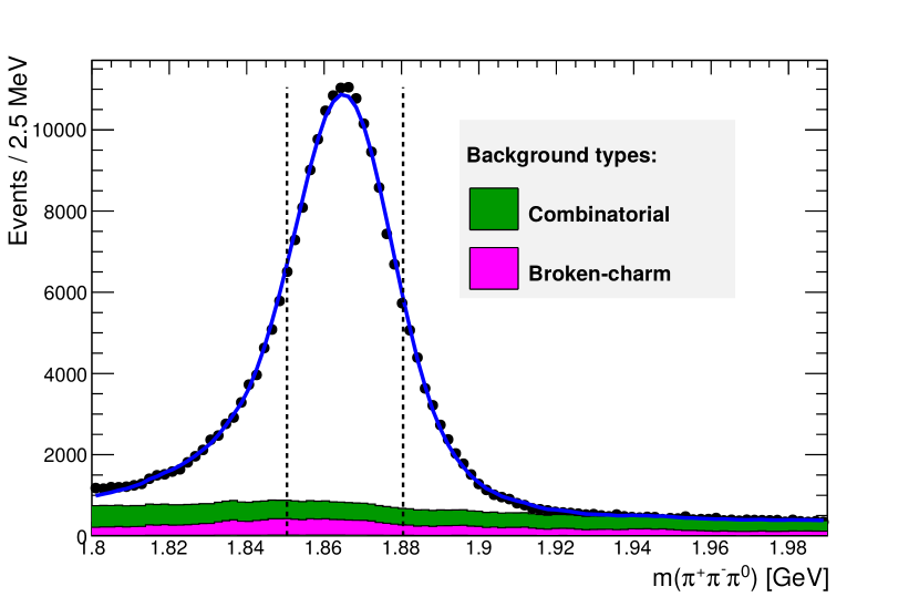
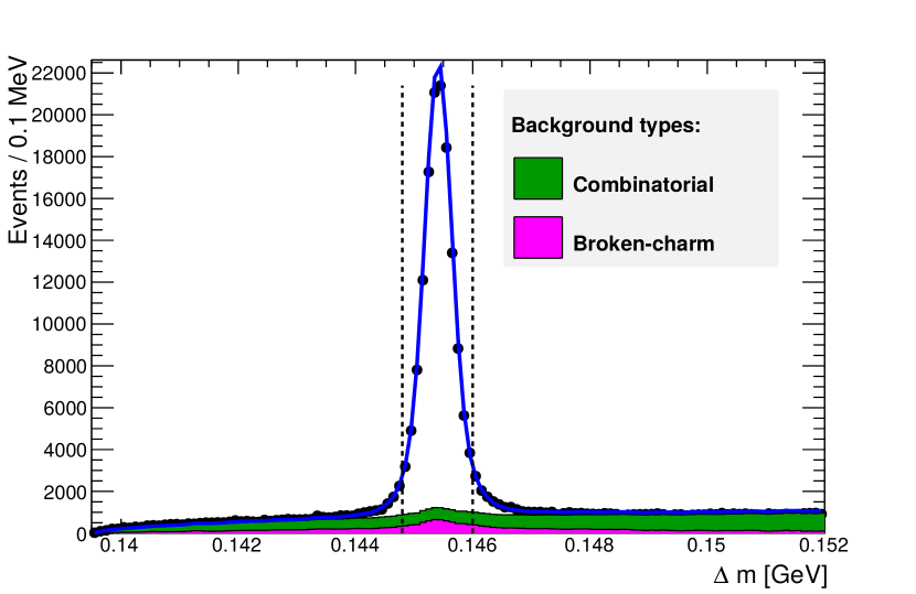
Figure 1: (Color online). (a) The reconstructed $D^{0}$ mass distribution of data (dots) with its fit projection (blue line), requiring $\left|\Delta m-\Delta m_{\rm PDG}\right|<0.6$ $\mathrm{\,Me\kern-1.00006ptV}$; (b) The $\Delta m$ distribution of data (dots) with its fit projection (blue line), requiring $\left|m(\pi^{+}\pi^{-}\pi^{0})-m_{D^{0}}\right|<15$ $\mathrm{\,Me\kern-1.00006ptV}$. The underlying histograms shown in shaded bands represent contributions from different background categories defined in Section IV. The vertical dashed lines mark the actual $m(\pi^{+}\pi^{-}\pi^{0})$ or $\Delta m$ requirement for the DP analysis.

IV Measurement of the mixing parameters

IV.1 Fit Model

The mixing parameters are extracted through a fit to the DP distribution of the selected events as a function of time $t$. The data is fit with a total PDF which is the sum of three component PDFs describing the signal, “broken-charm” backgrounds, and combinatorial background.

The signal DP distribution is parametrized in terms of an isobar model Fleming (1964); Morgan (1968); Herndon et al. (1975). The total amplitude is a coherent sum of partial waves $\mathcal{W}_{k}$ with complex weights $c_{k}$,

$$\overline{A}_{f}(s_{-},s_{+})=A_{f}(s_{+},s_{-})=\sum_{k}{c_{k}\mathcal{W}_{k}(s_{+},s_{-})}\,,$$ (3)

where $A_{f}$ and $\overline{A}_{f}$ are the final state amplitudes introduced in Eq. (1). Our model uses relativistic Breit-Wigner functions each multiplied by a real spin-dependent angular factor using the same formalism with the Zemach variation as described in Ref. Kopp et al. (2001) for $\mathcal{W}_{k}$, and constant $\mathcal{W}_{\rm{NR}}=1$ for the non-resonant term. As in Ref. Kopp et al. (2001), $\mathcal{W}_{k}$ also includes the Blatt-Weisskopf form factors with the radii of $D^{0}$ and intermediate resonances set at 5 $\mathrm{\,Ge\kern-1.00006ptV}^{-1}$ and 1.5 $\mathrm{\,Ge\kern-1.00006ptV}^{-1}$, respectively. The CLEO collaboration modeled the decay as a coherent combination of four amplitudes: those with intermediate $\rho^{+},\rho^{0},\rho^{-}$ resonances and a uniform non-resonant term Cronin-Hennessy et al. (2005). This form works well to describe lower statistics samples. In this analysis we use the model we developed for our higher statistics search for time-integrated $C\!P$ violation Aubert et al. (2007b), which also includes other resonances as listed in Table 1. The partial wave with a $\rho^{+}$ resonance is the reference amplitude. The true decay time distribution at any point in the DP depends on the amplitude model and the mixing parameters. We model the observed decay time distribution at each point in the DP as an exponential with average decay time coming from the mixing formalism (Eq. (1)) convolved with the decay time resolution, modeled as the sum of three Gaussians with widths proportional to $\sigma_{t}$ and determined from simulation. As the ability to reconstruct $t$ varies with the position in the DP, our parameterization of the signal PDF includes $\sigma_{t}$ functions that depend on $m^{2}(\pi^{+}\pi^{-})$, defined separately in six ranges, each as an exponential convolved with a Gaussian. Efficiency variations across the Dalitz-plot are modeled by a histogram obtained from simulated decays generated with a uniformly populated phase space.

In addition to correctly reconstructed signal decay chains, a small fraction of the events, $<\,1$%, contain $D^{0}\rightarrow\pi^{+}\pi^{-}\pi^{0}$ ($\kern 1.99997pt\overline{\kern-1.99997ptD}{}^{0}\rightarrow\pi^{+}\pi^{-}\pi^{0}$) decays which are correctly reconstructed, but then paired with false slow pion candidates to create fake $D^{*+}$ ($D^{*-}$) candidates. As these are real $D^{0}$ decays, their DP and decay time distributions are described in the fit assuming a randomly tagged flavor. The total amplitude for this contribution is $A^{\prime}_{f}(s+,s-)=f_{\rm RS}A_{f}(s+,s-)+(1-f_{\rm RS})A_{f}(s-,s+)$, where $f_{\rm RS}$ is the “lucky fraction” that we have a fake slow pion with the correct charge. As roughly half of these events are assigned the wrong $D$ flavor, we set $f_{\rm RS}=50\%$ in the nominal fit. We later vary this fraction to determine a corresponding systematic uncertainty.

Backgrounds from mis-reconstructed signal decays and other $D^{0}$ decays are referred to as “broken-charm”. In the fit, the Dalitz-plot distribution for this category is described by histograms taken from the simulations. The decay time distributions are described by the sum of two exponentials convolved with Gaussians whose parameters are taken from fits to the simulations.

We use sideband data to estimate combinatorial background. The data are taken from the sidebands with $m\left(\pi^{+}\pi^{-}\pi^{0}\right)<1.80\mathrm{\,Ge\kern-1.00006ptV}$ or $m\left(\pi^{+}\pi^{-}\pi^{0}\right)>1.92\mathrm{\,Ge\kern-1.00006ptV}$, and outside of the region $0.144<\Delta m<0.147$ $\mathrm{\,Ge\kern-1.00006ptV}$, where most of the broken-charm background events reside. The weighted sum of the two sideband regions is used to describe the combinatorial background in the signal region. The sideband weights and their uncertainties are determined from full MC simulation. We model these events in $t$ similarly to the broken-charm category. The decay time is described by the sum of two exponentials convolved with Gaussians. As an ad hoc description of $\sigma_{t}$ between 0 and 0.8 ps, the $\sigma_{t}$ function for the combinatorial background is an exponential convolved with a Gaussian, but we use different values in six ranges of $\left|t\right|$.

The best-fit parameters are determined by an unbinned maximum-likelihood fit. The central values for $x$ and $y$ were blinded until the systematic uncertainties were estimated. Because of the high statistics and the complexity of the model, the fit is computationally intensive. We have therefore developed an open-source framework called GooFit Andreassen et al. (2014) to exploit the parallel processing power of graphical processing units. Both the framework and the specific analysis code used in this analysis are publicly available .

IV.2 Fit Results

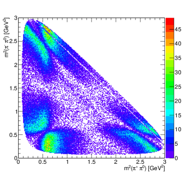
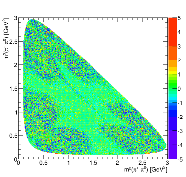
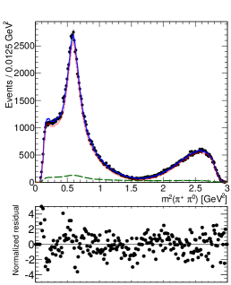
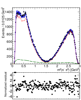
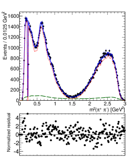
Figure 2: (Color online). The (a) Dalitz-plot and (b) difference between the Dalitz-plot and fit model prediction normalized by the associated statistical uncertainty in each bin, both time-integrated for the data. Also shown underneath are the projections of (c) $m^{2}_{\pi^{+}\pi^{0}}$, (d) $m^{2}_{\pi^{-}\pi^{0}}$, and (e) $m^{2}_{\pi^{+}\pi^{-}}$ for our data (points) and fit model (blue solid lines), together with the fit residuals normalized by the associated statistical uncertainties. The PDF components for signal (red dotted) and background (green dashed) events are shown. Note the narrow gap in (e) due to the $K^{0}_{\scriptscriptstyle S}$ veto.

The time-integrated Dalitz-plot for the signal region data is shown in Fig. 2. The amplitude parameters determined by the fit described above are listed in Table 1. Our amplitude parameters and the associated fractions are generally consistent with the previous BABAR results based on a subset of our data Aubert et al. (2007b). The normalized difference between the signal DP and the model is shown in Fig. 2. The $m^{2}(\pi^{\pm}\pi^{0})$ and $m^{2}(\pi^{+}\pi^{-})$ projections of the data and model are shown in Fig. 2(c)–(e). Differences between the data and the fit model are apparent in both the Dalitz-plot itself and the projections. Large pull values are observed predominantly near low and high values of $m^{2}$ in all projections. However, we understand the origin of these discrepancies, and the systematic uncertainties induced on the mixing parameters are small, as discussed below. Our fit reports the raw mixing parameters as $x=(2.08\pm 1.17)\%$ and $y=(0.14\pm 0.89)\%$. The correlation coefficient between $x$ and $y$ is $-0.6$%. The measured $D^{0}$ lifetime is $\tau_{D}=(410.2\pm 3.8){\rm{\,fs}}$, and agrees with the world average of $(410.1\pm 1.5)$ fs Olive et al. (2014). The central values of $x$ and $y$ are later corrected by the estimated fit biases as discussed in Sec. V.

Table 1: Results of the fit to the $D^{0}\rightarrow\pi^{+}\pi^{-}\pi^{0}$ sample showing each resonance amplitude magnitude, phase, and fit fraction $f_{r}\equiv\int{\left|c_{k}A_{k}\left(s_{+},s_{-}\right)\right|^{2}ds_{-}ds_{+}}$. The uncertainties are statistical only. We take the mass (width) of the $f_{0}(500)$ to be 500 (400) $\mathrm{\,Me\kern-1.00006ptV}$. In the fit, all resonance masses and widths are fixed to the listed values, which are taken from earlier world averages produced by the Particle Data Group Olive et al. (2014).

	Resonance parameters			Fit to data results
State	$J^{PC}$	Mass ($\mathrm{\,Me\kern-1.00006ptV}$)	Width ($\mathrm{\,Me\kern-1.00006ptV}$)	Magnitude	Phase (∘)	Fraction $f_{r}$ (%)
$\rho(770)^{+}$	$1^{--}$	775.8	150.3	1	0	$66.4\pm 0.5$
$\rho(770)^{0}$	$1^{--}$	775.8	150.3	$0.55\pm 0.01$	$16.1\pm 0.4$	$23.9\pm 0.3$
$\rho(770)^{-}$	$1^{--}$	775.8	150.3	$0.73\pm 0.01$	$-1.6\pm 0.5$	$35.6\pm 0.4$
$\rho(1450)^{+}$	$1^{--}$	1465	400	$0.55\pm 0.07$	$-7.7\pm 8.2$	$1.1\pm 0.3$
$\rho(1450)^{0}$	$1^{--}$	1465	400	$0.19\pm 0.07$	$-70.4\pm 15.9$	$0.1\pm 0.1$
$\rho(1450)^{-}$	$1^{--}$	1465	400	$0.53\pm 0.06$	$8.2\pm 6.7$	$1.0\pm 0.2$
$\rho(1700)^{+}$	$1^{--}$	1720	250	$0.91\pm 0.15$	$-23.3\pm 10.3$	$1.5\pm 0.5$
$\rho(1700)^{0}$	$1^{--}$	1720	250	$0.60\pm 0.13$	$-56.3\pm 16.0$	$0.7\pm 0.3$
$\rho(1700)^{-}$	$1^{--}$	1720	250	$0.98\pm 0.17$	$78.9\pm 8.5$	$1.7\pm 0.6$
$f_{0}(980)$	$0^{++}$	980	44	$0.06\pm 0.01$	$-58.8\pm 2.9$	$0.3\pm 0.1$
$f_{0}(1370)$	$0^{++}$	1434	173	$0.20\pm 0.03$	$-19.6\pm 9.5$	$0.3\pm 0.1$
$f_{0}(1500)$	$0^{++}$	1507	109	$0.18\pm 0.02$	$7.4\pm 7.4$	$0.3\pm 0.1$
$f_{0}(1710)$	$0^{++}$	1714	140	$0.40\pm 0.08$	$42.9\pm 8.8$	$0.3\pm 0.1$
$f_{2}(1270)$	$2^{++}$	1275.4	185.1	$0.25\pm 0.01$	$8.8\pm 2.6$	$0.9\pm 0.1$
$f_{0}(500)$	$0^{++}$	500	400	$0.26\pm 0.01$	$-4.1\pm 3.7$	$0.9\pm 0.1$
$NR$				$0.43\pm 0.07$	$-22.1\pm 11.7$	$0.4\pm 0.1$

V Systematic Uncertainties

Table 2: Summary of systematic uncertainties. The various sources are added in quadrature to find the total systematic uncertainty.

Source	$x$ [%]	$y$ [%]
“Lucky” false slow pion fraction	0.01	0.01
Time resolution dependence	0.03	0.02
on reconstructed $D^{0}$ mass
Amplitude-model variations	0.31	0.12
Resonance radius	0.02	0.10
DP efficiency parametrization	0.03	0.03
DP normalization granularity	0.03	0.04
Background DP distribution	0.21	0.11
Decay time window	0.18	0.19
$\sigma_{t}$ cutoff	0.01	0.01
Number of $\sigma_{t}$ ranges	0.11	0.26
$\sigma_{t}$ parametrization	0.05	0.03
Background-model MC time	0.06	0.11
distribution parameters
Fit bias correction	0.29	0.02
SVT misalignment	0.20	0.23
Total	0.56	0.46

Most sources of systematic uncertainty are studied by varying some aspect of the fit, measuring the resulting $x$ and $y$ values, and taking the full differences between the nominal and the varied results as the corresponding systematic uncertainty.

To study instrumental effects that may not be well-simulated and are not covered in other studies, we divide the data into four groups of disjoint bins and calculate $\chi^{2}$ with respect to the overall average for each group for both $x$ and $y$. Within a group, each bin has roughly the same statistics. Four bins of $m(\pi^{+}\pi^{-}\pi^{0})$ give $\chi^{2}=3.9$ (0.2) for $x$ ($y$); five bins of each of $D^{0}$ laboratory momentum $p_{\rm lab}$, $\cos\theta$, and $\phi$ give $\chi^{2}$ values of 1.5, 1.2, and 3.2 (5.9, 5.1, and 6.9) for $x$ ($y$), respectively. Altogether, the summed $\chi^{2}$ is 27.9 for $\nu=37$ degrees of freedom. Ignoring possible correlations, the $p$-value for the hypothesis that the variations are consistent with being purely statistical fluctuations around a common mean value is $\approx 85\%$. Therefore, we assign no additional systematic uncertainties.

Table 2 summarizes the systematic uncertainties described in detail below. Combining them in quadrature, we find total systematic uncertainties of 0.56% for $x$ and 0.46% for $y$.

As mentioned earlier, one source of background comes from events in which the $D^{0}$ is correctly reconstructed, but is paired with a random slow pion. We assume the lucky fraction $f_{\rm RS}$ to be exactly $50\%$ in the nominal fit. To estimate the uncertainty associated with this assumption, we vary the fraction from 40% to 60% and take the largest variations as an estimate of the uncertainty.

The detector resolution leads to correlations between reconstructed $D^{0}$ mass and the decay time, $t$. We divide the sample into four ranges of $D^{0}$ mass with approximately equal statistics and fit them separately; we find the variations consistent with statistical fluctuations. Because the average decay time is correlated with the reconstructed $D^{0}$ mass, we refit the data by introducing separate time resolution functions for each range, allowing the sets of parameters to vary independently. The associated systematic uncertainties are taken as the differences from the nominal values.

The DP distribution of the signal is modeled as a coherent sum of quasi-two-body decays, involving several resonances. To study the sensitivity to the choice of the model, we remove some resonances from the coherent sum. To decide if removing a resonance provides a “reasonable” description of the data, we calculate the $\chi^{2}$ of a fit using an adaptive binning process where each bin contains at least a reasonable number of events so that its statistical uncertainty is well determined. With 1762 bins, the nominal fit has $\chi^{2}=2794$. We separately drop the four partial waves that individually increase $\chi^{2}$ by less than 80 units: $f_{0}(1370)$, $f_{0}(1500)$, $f_{0}(1710)$, and $\rho(1700)$. We take the largest variations as the systematic uncertainties. The other partial waves individually when removed produce $\Delta\chi^{2}>$ 165. Additional uncertainties from our amplitude model due to poor knowledge of the mass and width of $f_{0}(500)$ are accounted for by floating the mass and width of $f_{0}(500)$ in the fit to data and taking the variations in $x$ and $y$. The default resonance radius used in the Breit-Wigner resonances in the isobar components is 1.5 $\mathrm{\,Ge\kern-1.00006ptV}^{-1}$, as mentioned earlier. We vary it in steps of 0.5 $\mathrm{\,Ge\kern-1.00006ptV}^{-1}$ from a radius of 0 to 2.5 $\mathrm{\,Ge\kern-1.00006ptV}^{-1}$ and again take the largest variations.

The efficiency as a function of position in the DP in the nominal fit is modeled using a histogram taken from events generated with a uniform phase space distribution. As a variation, we parameterize the efficiency using a third-degree polynomial in $s_{+},s_{-}$ and take the difference in mixing parameters as the uncertainty in the efficiency model. Normalization over the DP is done numerically by evaluating the total PDF on a $120\times 120$ grid. To find the sensitivity to the accuracy of the normalization integral, we vary the granularity of the grid from $120\times 120$ to $240\times 240$ and take the largest variations as systematic uncertainties. The combinatorial background in the DP is modeled by sideband data summed according to weights taken from simulation. We repeat the fit using a histogram taken from simulation and vary the weights by $\pm 1$ standard deviation. Additionally, we vary the number of bins used in the “broken-charm” histograms.

In the nominal fit, we consider events in the decay time window between $-2$ and $+3$ ps, $\textit{i}.\textit{e}.$ about $-5$ to $+7$ $\tau_{D^{0}}$. To test our sensitivity to high-$|t|$ events, the window is varied, with the low end ranging from $-$3.0 ps to $-$1.5 ps and the high end ranging from 2.0 ps to 3.0 ps. We assign an uncertainty of 0.18% to $x$ and 0.19% to $y$, the largest variations from this source. We vary the maximum allowed uncertainty on the reconstructed decay time $\sigma_{t}$ to study the effect of poorly measured events. The nominal cutoff at 0.8 ps is relaxed to 1.2 ps in steps of 0.1 ps and we use the largest variations as the uncertainties from this source. To account for the variation of $\sigma_{t}$ across the DP, the nominal fit has six different $\sigma_{t}$ distributions, one for each range of $m^{2}(\pi^{+}\pi^{-})$. We reduce the number of ranges to two and increase it to eight, and use the largest difference as the uncertainty associated with the number of ranges. Additionally, instead of using a functional form to describe the $\sigma_{t}$ distribution in each range, we repeat our nominal fit using a histogram taken from simulation. This produces extremely small changes in the measured mixing parameters; we take the full difference as an estimate of the uncertainty.

In the nominal fit, the background components have their decay time dependences modeled by the sums of two exponentials convolved with Gaussians whose parameters are fixed to values found from fits to simulated data. We vary each parameter in sequence by $\pm 1$ standard deviation and take the largest variations as estimates of the systematic uncertainty.

Our fits combine two effects: detector resolution and efficiency. We ignore the migration of events which are produced at one point in the DP and reconstructed at another point; we parameterize detection efficiency from simulated events, generated with a uniformly populated DP using the observed positions, in the numerator. As noted earlier, this leads to discrepancies between fit projections and data for simulated data which are very similar to those observed for real data as observed in Fig. 2. We believe this is due to ignoring the systematic migration of events away from the boundaries of phase space induced by misreconstruction followed by constrained fitting. We have further checked the migration effect by fitting the data in a smaller DP phase space with all the boundaries shifted 0.05 $\mathrm{\,Ge\kern-1.00006ptV}^{2}$ inwards. In addition, detector resolution leads to a correlation between reconstructed $D^{0}$ mass and $t$, also noted earlier. To estimate the level of bias and systematic uncertainty introduced by these factors, we studied the full MC samples described in Section III. The fit results display small biases in $x$ and $y$. From the fit to each sample, we determine the pull values for $x$ and $y$, defined as the differences of fitted and input values. We then correct for fit biases by subtracting $+0.58\%$ from $x$ and $-0.05$% from $y$ where the numerical values are the mean deviations from the generated values. The assigned systematic uncertainties are half the shifts in each variable.

To test the sensitivity of our results to small uncertainties in our knowledge of the precise positions of the SVT wafers, we reconstruct some of our MC samples with deliberately wrong alignment files that produce much greater pathologies than are evident in the data. We again create background mixtures and fit these misaligned samples. Four samples are generated, all with $x=y=+1\%$. Each sample has roughly the same magnitude of effect caused by the five different misalignments considered. As the misalignments used in this study are extreme, we estimate the systematic uncertainties as half of the averages of the absolute values of the shifts in $x$ and $y$.

VI Summary and conclusions

We have presented the first measurement of $D^{0}$–$\kern 1.99997pt\overline{\kern-1.99997ptD}{}^{0}$ mixing parameters from a time-dependent amplitude analysis of the decay $D^{0}\rightarrow\pi^{+}\pi^{-}\pi^{0}$. We find $x=(1.5\pm 1.2\pm 0.6)\%$ and $y=(0.2\pm 0.9\pm 0.5)\%$, where the quoted uncertainties are statistical and systematic, respectively. The dominant sources of systematic uncertainty can be reduced in analyses with larger data sets. Major sources of systematic uncertainty in this measurement include those originating in how we determine shifts for detector misalignment and the choice of decay time window. We estimated conservatively the former as it is already small compared to the statistical uncertainty of this measurement. The latter can be reduced by more carefully determining the signal-to-background ratio as a function of decay time. However, since the systematic uncertainties are already small compared to the statistical uncertainties, we choose not to do so in this analysis. Similar considerations suggest that systematic uncertainties will remain smaller than statistical uncertainties even when data sets grow to be 10 to 100 times larger in experiments such as LHCb and Belle II.

VII Acknowledgments

We are grateful for the extraordinary contributions of our PEP-II colleagues in achieving the excellent luminosity and machine conditions that have made this work possible. The success of this project also relies critically on the expertise and dedication of the computing organizations that support BABAR. The collaborating institutions wish to thank SLAC for its support and the kind hospitality extended to them. This work is supported by the US Department of Energy and National Science Foundation, the Natural Sciences and Engineering Research Council (Canada), the Commissariat à l’Energie Atomique and Institut National de Physique Nucléaire et de Physique des Particules (France), the Bundesministerium für Bildung und Forschung and Deutsche Forschungsgemeinschaft (Germany), the Istituto Nazionale di Fisica Nucleare (Italy), the Foundation for Fundamental Research on Matter (The Netherlands), the Research Council of Norway, the Ministry of Education and Science of the Russian Federation, Ministerio de Economía y Competitividad (Spain), the Science and Technology Facilities Council (United Kingdom), and the Binational Science Foundation (U.S.-Israel). Individuals have received support from the Marie-Curie IEF program (European Union) and the A. P. Sloan Foundation (USA).

References

- Pais and Treiman (1975) A. Pais and S. B. Treiman, Phys. Rev. D 12, 2744 (1975).
- Aubert et al. (2007a) B. Aubert et al. (BABAR Collaboration), Phys. Rev. Lett. 98, 211802 (2007a).
- Starič et al. (2007) M. Starič et al. (Belle Collaboration), Phys. Rev. Lett. 98, 211803 (2007).
- Aaltonen et al. (2008) T. Aaltonen et al. (CDF Collaboration), Phys. Rev. Lett. 100, 121802 (2008).
- Aaij et al. (2013a) R. Aaij et al. (LHCb Collaboration), Phys. Rev. Lett. 110, 101802 (2013a).
- Aaij et al. (2013b) R. Aaij et al. (LHCb Collaboration), Phys. Rev. Lett. 111, 251801 (2013b).
- Aaij et al. (2016) R. Aaij et al. (LHCb Collaboration), arXiv:1602.07224 [hep-ex] (2016).
- Asner et al. (2005) D. M. Asner et al. (CLEO Collaboration), Phys. Rev. D 72, 012001 (2005).
- Abe et al. (2007) K. Abe et al. (Belle Collaboration), Phys. Rev. Lett. 99, 131803 (2007).
- del Amo Sanchez et al. (2010) P. del Amo Sanchez et al. (BABAR Collaboration), Phys. Rev. Lett. 105, 081803 (2010).
- Peng et al. (2014) T. Peng et al. (Belle Collaboration), Phys. Rev. D 89, 091103 (2014).
- Amhis et al. (2014) Y. Amhis et al. (Heavy Flavor Averaging Group (HFAG)), arXiv:1412.7515 [hep-ex] (2014), (May 2015 updated values taken from HFAG website.).
- Olive et al. (2014) K. Olive et al. (Particle Data Group), Chin.Phys. C38, 090001 (2014).
- Lees et al. (2013) J. P. Lees et al. (BABAR Collaboration), Nucl. Instr. Meth. Phys. Res., Sect. A 726, 203 (2013).
- Aubert et al. (2002) B. Aubert et al. (BABAR Collaboration), Nucl. Instr. Meth. Phys. Res., Sect. A 479, 1 (2002).
- Aubert et al. (2013) B. Aubert et al. (BABAR Collaboration), Nucl. Instr. Meth. Phys. Res., Sect. A 729, 615 (2013).
- Aubert et al. (2006) B. Aubert et al. (BABAR Collaboration), Phys. Rev. D 74, 091102 (2006).
- Aubert et al. (2007b) B. Aubert et al. (BABAR Collaboration), Phys. Rev. Lett. 99, 251801 (2007b).
- Albrecht et al. (1990) H. Albrecht et al. (ARGUS), Z. Phys. C48, 543 (1990).
- Fleming (1964) G. N. Fleming, Phys. Rev. 135, B551 (1964).
- Morgan (1968) D. Morgan, Phys. Rev. 166, 1731 (1968).
- Herndon et al. (1975) D. J. Herndon et al., Phys. Rev. D 11, 3165 (1975).
- Kopp et al. (2001) S. Kopp et al. (CLEO), Phys. Rev. D 63, 092001 (2001).
- Cronin-Hennessy et al. (2005) D. Cronin-Hennessy et al. (CLEO Collaboration), Phys. Rev. D 72, 031102 (2005).
- Andreassen et al. (2014) R. Andreassen et al., IEEE Access 2, 160 (2014).