Spontaneous concentrations of solids through
two-way drag forces between gas and sedimenting particles

The behaviour of sedimenting particles depends on the dust-to-gas ratio of the fluid. Linear stability analysis shows that solids settling in the Epstein drag regime would remain homogeneously distributed in non-rotating incompressible fluids, even when dust-to-gas ratios reach unity. However, the non-linear evolution has not been probed before. Here, we present numerical calculations indicating that in a particle-dense mixture solids spontaneously mix out of the fluid and form swarms overdense in particles by at least a factor $10$. The instability is caused by mass-loaded regions locally breaking the equilibrium background stratification. The driving mechanism depends on non-linear perturbations of the background flow and shares some similarity to the streaming instability in accretion discs. The resulting particle-rich swarms may stimulate particle growth by coagulation. In the context of protoplanetary discs, the instability could be relevant for aiding small particles to settle to the midplane in the outer disc. Inside the gas envelopes of protoplanets, enhanced settling may lead to a reduced dust opacity, which facilitates the contraction of the envelope. We show that the relevant physical set up can be recreated in a laboratory setting. This will allow our numerical calculations to be investigated experimentally in the future.

1 Introduction

The study of gas drag on mm to dm-sized particles (pebbles) is essential to understand the formation of planets. Vertical sedimentation due to drag on small particles in the protoplanetary disc is necessary for the creation of a dense midplane of solids from which larger objects can grow (Youdin & Lithwick 2007). Conversely, the same drag force is also responsible for the rapid radial migration of pebbles in the midplane (on $100$ yr time scales in the terrestrial region, Weidenschilling 1977). This is the main barrier for continued growth to larger than cm to m sizes by collisions (Brauer et al. 2008; Birnstiel et al. 2012), unless particles can have extremely low internal densities (Kataoka et al. 2013; Krijt et al. 2015).

The radial drift hurdle can be avoided through two mechanisms that also critically rely on gas drag. Firstly, pebbles can be concentrated hydrodynamically, so that the resulting clouds collapse gravitationally to planetesimals of $\sim$$100$ km in size (for recent reviews on different planetesimal formation models, see Johansen et al. 2014; Chiang & Youdin 2010). Secondly, large planetesimals can accrete the remaining drifting pebbles and grow to planetary sizes (Lambrechts & Johansen 2012, 2014; Guillot et al. 2014).

Not only the drag on the particles is important, but also the backreaction of the particles on the gas. Initially, it was proposed that a secular instability on a settled dust layer could lead to local particle pileups (Goodman & Pindor 2000). The pileup would originate from a process resembling plate drag, where the drag force is assumed to collectively act on a monolithic particle midplane. This assumption is nevertheless questionable (Youdin & Chiang 2004) and numerical studies (Weidenschilling 2006) have not recovered the instability proposed by Goodman & Pindor (2000). Nevertheless, this work paved the way for a further investigation on the role of the backreaction force from gas drag. Youdin & Goodman (2005) identified a linear instability in the disc midplane. Their breakthrough result demonstrated that infinitesimal perturbations grow on an orbital time-scale when the dust-to-gas ratio is around unity or higher. This instability leads to spontaneous particle clumping, triggering the gravitational collapse that results in the formation of planetesimals. In a series of papers (Youdin & Johansen 2007; Johansen & Youdin 2007; Johansen et al. 2009, 2012) the linear and non-linear evolution of this instability were numerically investigated in detail. These results were independently confirmed and further explored by several other groups (Bai & Stone 2010a, b, c; Miniati 2010; Kowalik et al. 2013).

Several criteria for the streaming instability to achieve particle clumping have been identified:

• a disc with slightly supersolar dust-to-gas ratio (Johansen et al. 2009; Bai & Stone 2010c),

• particles of Stokes number $\tau_{\rm f}\sim 0.05$–$0.5$, approximately between mm and dm in size (Johansen & Youdin 2007; Bai & Stone 2010a, c; Carrera et al. 2015) and

• low radial pressure support in the disc (Bai & Stone 2010c).

Further investigations are moving towards a more global understanding of the effects of the streaming instability, by expanding the simulation domain in the azimuthal (Kowalik et al. 2013) or vertical direction (Yang & Johansen 2014). Additionally the streaming instability is placed in a larger context by incorporating magnetized turbulence (Johansen et al. 2007), dust coagulation models (Dra̧żkowska & Dullemond 2014) or vortex formation (Raettig et al. 2015).

In this paper we take a step back and study the general process of particle sedimentation in flows with a dust loading comparable to the gas density. The aim is twofold. Firstly, we hope to gain theoretical insight into particle sedimentation and more complex drag instabilities, such as the streaming instability and the photoelectric instability (Lyra & Kuchner 2013). Secondly, the sedimentation of particles is accessible to laboratory experiments, thus allowing for a potential experimental confirmation of a particle drag instability.

Of specific interest is the question whether any particle clumping will even occur at all in a mass-loaded particle rain. From previous analytic work on the streaming instability, we do not expect a linear instability to be present, because of the lack of rotation in a pure sedimentation problem. This removes the Coriolis force which is deemed necessary for the streaming instability to operate (Jacquet et al. 2011; Youdin & Goodman 2005). Nevertheless, in our physical set up (described in Section 2) a non-linear drafting instability is clearly present. The results are described in Section 3. The implications of this instability are discussed for particle sedimentation in protoplanetary discs, chondrule formation, and the envelopes of giant planets (Section 4). We also place our results in the context of planned laboratory experiments (Section 5.1). We summarise our findings in Section 6.

2 Mass-loaded particle rain

2.1 Model equations

We study the differential motion between particles initially moving with terminal velocity and stationary gas in hydrostatic balance. The dynamics of the gas component is described by

$$\partial_{t}\rho+\nabla\cdot(\rho\mbox{\boldmath{$u$}}) =0,$$ (1)

$$\partial_{t}\mbox{\boldmath{$u$}}+\mbox{\boldmath{$u$}}\nabla\cdot\mbox{\boldmath{$u$}} =-g\mbox{\boldmath{$e$}}_{z}-\frac{1}{\rho}\nabla P+\frac{1}{t_{\rm f}}\epsilon(\mbox{\boldmath{$v$}}-\mbox{\boldmath{$u$}})+\nu\nabla^{2}\mbox{\boldmath{$u$}},$$ (2)

where $\rho$ is the gas density, $u$ the gas velocity, $g$ the gravitational acceleration, $P$ the pressure, $\epsilon=\rho_{\rm p}/\rho$ is the local dust-to-gas ratio, $v$ the particle fluid velocity and $\nu$ the viscosity. The drag term from the particles onto the gas depends on the friction time of the particle (in the Epstein drag regime, Epstein 1924),

$$t_{\rm f}=\frac{\rho_{\bullet}R}{\rho v_{\rm th}}\,,$$ (3)

where $R,\rho_{\bullet}$ are the radius and solid density of the particle. The thermal velocity $v_{\rm th}$ is approximately equal to the local, isothermal gas sound speed $v_{\rm th}=\sqrt{8/\pi}c_{\rm s}$.

We investigate a regime where we assume an efficient coupling between particles and gas. In this case, the viscous diffusion time for momentum transport between an average particle pair located a distance $l_{\rm pair}$ apart is shorter than the friction time of a single particle,

$$t_{\nu,{\rm pair}}=\frac{l_{\rm pair}^{2}}{\nu}=\frac{n_{\rm p}^{-2/3}}{\nu}<t_{\rm f},$$ (4)

with $n_{\rm p}$ the particle number density. The particles can then be described by a pressureless fluid (a formal derivation can be found in Jacquet et al. 2011) with continuity and momentum equation

$$\partial_{t}\rho_{\rm p}+\nabla\cdot(\rho_{\rm p}\mbox{\boldmath{$v$}}) =0,$$ (5)

$$\partial_{t}\mbox{\boldmath{$v$}}+\mbox{\boldmath{$v$}}\nabla\cdot\mbox{\boldmath{$v$}} =-g\mbox{\boldmath{$e$}}_{z}-\frac{1}{t_{\rm f}}(\mbox{\boldmath{$v$}}-\mbox{\boldmath{$u$}}).$$ (6)

In the remainder of the paper we will employ ‘friction units’: the friction time $t_{\rm f}$ as time unit and the friction length $l_{\rm f}=gt_{\rm f}^{2}$ as length unit. Velocities can then be expressed in units of terminal velocity $v_{\rm f}=gt_{\rm f}$. The criterion expressed in Eq. (4), for example, reduces to $n_{\rm p}^{\prime-2/3}/\nu^{\prime}<1$. We will preserve the prime notation in the following sections to explicitly denote quantities expressed in friction units.

The use of the friction time as unit of time is possible for the sedimentation problem, because there are no rotation terms that would necessarily introduce the additional time scale of the orbital Keplerian frequency, as is for example the case for the streaming instability (Youdin & Goodman 2005).

Expressed in friction units the model equations leave us with only three free dimensionless parameters:

• the viscosity, $\nu^{\prime}=\nu/(g^{2}t_{\rm f}^{3})$, which is the inverse of the Reynolds number ($Re$) in terms of the terminal velocity and the friction length,

• the sound speed, $c_{\rm s}^{\prime}=c_{\rm s}/(gt_{\rm f})$, which is the inverse of the Mach number ($Ma$) in terms of the terminal velocity, and

• the dust-to-gas ratio, $\epsilon$.

The latter is arguably the most important, because we desire to work in the incompressible limit ($Ma\ll 1$) and we face a lower bound on the viscosity imposed by the requirement for numerical stability.

A major benefit from this choice of units is that our calculations do not require us to specify a particle size (Eq. 3). Thus our results can be freely scaled to the desired particle size in the context of protoplanetary discs (Section 4) or a laboratory setting (Section 5.1).

2.2 Numerical implementation

In our numerical simulations, performed with the Pencil Code, we do not employ the particle fluid description used for the analytical calculations for our main results, but instead use a Lagrangian super-particle approach. Particles are implemented as super-particles that represent swarms of physical particles. This is important, especially in the non-linear regime where it is desirable to allow particle trajectory crossing and steep density gradients (Youdin & Johansen 2007). We have nevertheless used the particle fluid approach also numerically to verify some of our work in the linear regime. The assignment of drag forces on the particles and on the gas is further described in Youdin & Johansen (2007) and in Johansen & Youdin (2007). Drag is calculated on particles assuming a constant friction time. We have also made use of the block domain decomposition for particle load balancing amongst processors (Johansen et al. 2011).

For the initial condition, we set up a gas column in hydrostatic equilibrium, taking the drag from the particles on the gas into account. Particles are typically distributed randomly, with the possibility to add perturbations (discussed in more detail in Section 3.1) and initiated with with their vertical velocity equal to the terminal velocity. The gas stratification then takes the form

$$\rho =\left(\rho_{p}+\rho_{\rm b}\right)\exp\left(-\frac{g}{c_{s}^{2}}z\right)-\rho_{p},$$ (7)

see Appendix A for more details. This initial condition works well, but we nevertheless find that in heavily elongated simulation domains, the stratification of the gas combined with a uniform particle distribution triggers a vertical gas density wave, that dissipates over time. There is also a small upwards advection of gas as the top of the domain gets cleared of particles. These effects restricts our simulation domain in practice to approximately $20$  $l_{\rm f}$ in the vertical direction (at $c_{\rm s}/v_{\rm f}=10$).

A full list of the performed simulations can be found in Table 1 and Table 2. Below, we describe the nominal numerical set up in detail.

The boundary condition are set to be periodic in the horizontal direction, for both the particle and gas component. In the vertical direction particles are removed from the simulation when crossing the edge of the simulated domain. The vertical boundary condition on the gas is symmetric (vanishing first derivative) in all quantities, except for the vertical gas velocity which is antisymmetric (vanishing value). This boundary condition effectively puts a solid surface at the bottom of the simulation domain, on which the gas is supported.

We use an ideal gas equation of state with adiabatic index $\gamma=5/3$. The sound speed is set to be $c_{\rm s}=10v_{\rm f}$ (unless mentioned otherwise) to approach the incompressible limit. The Pencil Code is a code optimised for both subsonic and mildly transsonic flows, but we found a Mach number of $0.1$ sufficient to probe the incompressible regime of interest.

We found a choice of 16 superparticles per grid cell is sufficiently high to model a coherent fluid and reduce particle noise (see also Appendix C). We have standardly used a physical viscosity treatment, but for runs with extended domain and high mass loading (run1.01, run1.02) we added sixth order ‘artificial viscosity’ (Haugen & Brandenburg 2004). We employed the minimal amount necessary to prevent numerical artefacts from developing. The grid Reynolds number is minimally $32$ times smaller than the Reynolds number in friction units. Most simulations were performed in 2 dimensions, but we have verified our results in 3 dimensions as well (run3d.4, Fig. 2), showing little difference. Nevertheless, such numerically expensive 3D runs are of interest for further study.

Table 1: Parameters of the numerical simulations. All values are given in the friction unit system. Here, $\nu$ is the viscosity, $\epsilon_{0}$ is the background dust-to-gas ratio, $c_{\rm s}$ is the sound speed, $A$ and $\lambda$ are the values of the amplitude and wavelength of the perturbation. The total number of particles is $N_{\rm par}$ and $N_{\rm cells}$ is the total number of grid cells.

Name	$L_{x}\times L_{z}$	Resolution	$\nu$	$\epsilon_{0}$	$c_{\rm s}$	Perturb.	$A$	$\lambda$	$N_{\rm par}/N_{\rm cells}$
run1	$1\times 20$	$32\times 640$	1.0e-4	1	10	rand	–	–	16
run2	$1\times 20$	$64\times 1280$	1.0e-4	1	10	rand	–	–	16
run3	$1\times 20$	$128\times 2560$	1.0e-4	1	10	rand	–	–	16
runRT	$1\times 20$	$32\times 640$	1.0e-4	1	10	$k_{\rm z}$	0.1	4	16
runKH	$2\times 20$	$64\times 640$	1.0e-4	1	10	$k_{\rm x}$	0.1	0.5	16
runEGG	$1\times 20$	$32\times 640$	1.0e-4	1	10	eggbox	0.1	1,4	16
runEGG2	$1\times 20$	$64\times 1280$	1.0e-4	1	10	eggbox	0.1	0.5,2	16
runv2	$1\times 20$	$32\times 640$	1.0e-2	1	10	rand	–	–	16
runv3	$1\times 20$	$32\times 640$	1.0e-3	1	10	rand	–	–	16
runv5	$1\times 20$	$32\times 640$	1.0e-5	1	10	rand	–	–	16
runv6	$1\times 20$	$32\times 640$	1.0e-5	1	10	rand	–	–	16
run1.e4	$1\times 20$	$32\times 640$	1.0e-4	1	10	rand	–	–	16
run2.n4	$1\times 20$	$64\times 1280$	1.0e-4	1	10	rand	–	–	4
run2.n64	$1\times 20$	$64\times 1280$	1.0e-4	1	10	rand	–	–	64
run3d.4	$1\times 1\times 20$	$32\times 32\times 640$	1.0e-4	4	10	rand	–	–	16

Table 2: Parameters of the numerical simulations extended in the vertical domain by $t_{\rm f}=0.1$. Values of variables in friction units (similar to Table 1). Here, art. visc. stands for the value of the artificial viscosity parameter.

Name	$L_{x}\times L_{z}$	Resolution	$\nu$	$\epsilon_{0}$	$c_{\rm s}$	Perturb.	A	$\lambda$	$N_{\rm par}/N_{\rm cells}$	art. visc.
run1.01	$100\times 2000$	$32\times 640$	1.0e-1	1	100	rand	–	–	16	$10$
run2.01	$100\times 2000$	$32\times 640$	1.0e-1	0.25	100	rand	–	–	16	$10$
run3.01	$100\times 2000$	$32\times 640$	1.0e-1	0.1	100	rand	–	–	16	–
run4.01	$100\times 2000$	$32\times 640$	1.0e-1	0.05	100	rand	–	–	16	–

3 Numerical results showing spontaneous particle concentrations

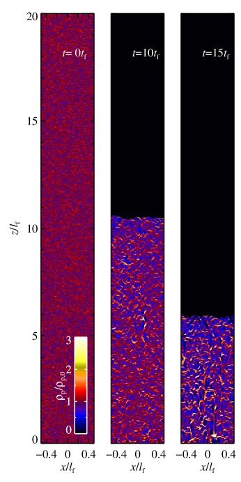
Figure 1: Development of particle swarms by a drafting instability. Displayed is the evolution of the particle density in the two-dimensional simulation run2 (see Table 1). The left-most panel illustrates the initial conditions: a stratified gas column in the vertical directions with particles sedimenting at terminal velocity, placed randomly throughout the simulation domain ($1$ $l_{\rm f}$ wide and $20$ $l_{\rm f}$ high, note that the figure aspect ratio is enlarged in the $x$-direction). In the following panels (time $t=10,15$ $t_{\rm f}$), regions marginally overdense with particles locally break the stratification equilibrium and accelerate downwards, while in particle-poor regions a deceleration from terminal velocity occurs. This leads to continued particle pileups through drafting, originating from gas being dragged by the particles. The particle and fluid components unmix and remain in this state. At the end of the simulation, when most particles have sedimented out of the simulation domain, the maximal particle density has increased by a factor $10$.

3.1 Nonlinear behaviour

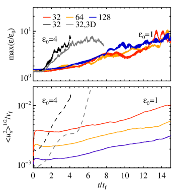
Figure 2: Top panel: Evolution of the particle density (normalized to the background dust-to-gas ratio $\epsilon_{0}$), for three different resolutions in 2D simulations and a 3D simulation (run3d.4, gray). Bottom panel: Evolution of the instability based on the horizontal gas dispersion, $\sqrt{<u_{x}^{2}>}$, (as an alternative tracer to the maximal particle density, which is an intrinsically noisy variable). We have used a similar color coding as top panel. Note for the runs with $\epsilon_{0}$$=$$4$ we have displaced the dashed curves for clarity with a factor 10 downwards.

From previous analytic studies of the streaming instability (Youdin & Goodman 2005; Jacquet et al. 2011), it is well known that rotation is an essential ingredient for the linear phase of particle clumping. The interpretation proposed by Jacquet et al. (2011) is that the Coriolis force is necessary to create a pressure maximum supported by geostrophic balance. We have repeated the analysis in Appendix A for completeness. It demonstrates that the sedimentation model without rotation discussed in this paper is not expected to show a linear instability, under the assumption of incompressible gas.

Our numerical results nevertheless show that even a minimal disturbance of the sedimenting particle component with $\epsilon=1$ leads to spontaneous clumping of material, resulting in the particles to unmix and sediment out of the fluid. Figure 1 illustrates the process. Particles located in initially weakly overdense regions sediment faster, dragging the gas along, resulting in a drafting effect which pulls in more particles. For clarity, the drafting mentioned here is the result of the collective motion of a swarm of particles and the resulting gas drag back reaction, not from individual particle slipstreaming. At the same time, the opposite occurs in regions less dense than the mean particle density. These effects amplify each other, which results in dense swarms of particles to form that can undergo secondary instabilities. For example, one can see in the bottom of the last panel of Fig. 1 a particle cloud resembling a characteristic Rayleigh-Taylor mushroom, which we will discuss in more detail below.

3.2 Particle noise perturbation

We begin by considering the evolution of the sedimenting particles, when they are placed randomly in the simulation domain. This corresponds to a noisy initial condition for the particle distribution, with maximal relative changes in the particle density on the order of $50$ % for our nominal 2D resolution, for more detail see Appendix C.

Figure 2 shows the time evolution of the maximal particle density in the simulated domain (for different background dust-to-gas ratios). Particle overdensities reach $10$ times the average value, although they are still growing slowly towards the end of the simulations when the particles fall out of the box. Over time, particles sediment out of the simulated domain, so at late times fewer and fewer particles are traced. For clarity, we also show the evolution of the horizontal gas velocity dispersion, which is a less noisy measurement than the particle density. This illustrates the exponential nature of the instability as well.

Our numerical results stand in contrast to the stable state predicted by linear stability analysis. It appears that the main driver for the particle clumping is an imbalanced stratification. Recall that the particle loading of the sedimenting particles is taken into account when setting up the equilibrium state (Eq.7). This balance can be broken along the $x$-direction by regions with a higher, or less high, particle density compared to the mean value. Apparently, the fluid and particles have no means of finding a global equilibrium state in the $x$-direction in the response to the particle fluctuation. Instead, the particle components breaks into dense swarms.

This interpretation is supported by the correlation between overdense regions and their increased settling speeds shown in Fig. 3. We have binned the surrounding gas and particle velocity in the grid cell for every particle in the simulation of run2, revealing that on average gas and particles sediment about $1$% of faster or slower for order unity fluctuations in the dust-to-gas ratio.

From inspection of our numerical results at different resolutions and spatial scales, we find that the instability tends to originate on the smallest available scale, near the grid scale in simulations with minimal viscosity (the dependency on the viscosity is discussed in Sec. 3.6 in more detail). This makes it computationally challenging to characterize the instability, as increased resolutions do not necessarily better resolve the characteristic scale of interest. Instead, the instability takes place a little faster and remains quantitatively similar (Fig. 2).

The view of the drafting instability as arising from an imbalanced pressure stratification suggests that the instability is non-linear, as the particle fluctuations that drive the horizontal imbalance must be seeded from the initial condition. This implies that the growth rate of the instability should decrease with increasing particle number, as randomly placed particles have a decreased effective density fluctuation with increased particle number. We show in Appendix C that indeed the fastest growth is found when reducing the particle number to just four per cell. However, we are not able to completely shut off the instability at larger particle number, indicating that the instability may operate even in the limit of very high particle number.

In the next sections we investigate how the sedimenting particles react to different perturbations of the system in order to gain further insight in the non-linear phase. We then propose that a toy model that can capture the dependency of the instability on the metallicity and Reynolds number (Sec. 3.5 – 3.6).

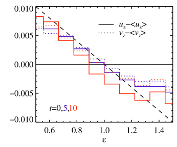
Figure 3: Correlation between the local dust-to-gas ratio $\epsilon$ and the deviations in the velocity of the gas $u_{\rm z}$ (full line) and particles $v_{\rm z}$ (dotted line). To aid interpretation, we subtracted the mean velocity of the sedimenting particles $\left<v_{z}\right>$ from the particle velocity and a small artificial upwards mean gas velocity $\left<u_{z}\right>$ from the gas velocity. Displayed are different times $t=0,5,10$ $t_{\rm f}$, in respectively black, blue and red, based on the region between $z$=$0$–$10$ $l_{\rm f}$ in run2. The standard deviations on the binned averages are relatively large, $\sigma$$\approx$$0.03$–$0.04$ $v_{\rm f}$ for the gas and particle velocities between $t$=$5$–$10$ $t_{\rm f}$. The black dashed line corresponds to $\alpha=0.02$ in the toy model (Sec. 3.5).

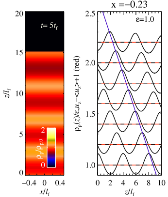
Figure 4: Left panel: Sedimenting particles with a $k_{\rm z}=\pi/2$-mode in the particle density. Represented is a snapshot of runRT at $t=5t_{\rm f}$. No instabilities develop, suggesting that the drafting instability is not directly related to the Rayleigh-Taylor instabilities that should occur in this set up. Right panel: Evolution of the sedimenting particle wave at an arbitrary placed slice at $x=-0.23$. Different curves represent different times ($t=0,1,2,\dots,6$ $t_{\rm f}$), that for clarity are offset by $0.2$. The particle density $\rho_{\rm p}(z)$ is given in black, while the red dashed line gives the gas velocity $u_{z}(z)$. Particle ridges do not approach each other, as indicated by the blue line that tracks the position of a point advected with velocity $v_{\rm f}$. The pressure that is supporting the mass-loaded stratification adapts to compensate for small changes in the particle density. This allows $u_{z}(z)$ to remain zero while the particles sediment.

3.3 Wave perturbation

We now verify numerically that the drafting instability is not related to either the Rayleigh-Taylor instability or the Kelvin-Helmholtz instability by perturbing the system with either a purely vertical or purely horizontal a vertical mode in the particle distribution.

We first present results of vertical wave perturbation of the particle density, which can be seen in Fig. 4. Within the time that particles sediment out of the domain, no instabilities can be detected. The right panel of Fig. 4 shows that the particles simply sediment at terminal velocity. At the same time, the gas component does not react to the perturbation. We have verified that this result even stands when feeding additional particle noise to the simulation. We do not see any Rayleigh-Taylor-like instabilities (that occur in a hydrostatic fluid with a dense layer on a lighter one, Drazin & Reid 2004). This experiment also demonstrates that the mechanism concentrating particles is at least two-dimensional. In 1D simulations with only a vertical perturbation the ridges of increased particle density do not approach each other.

We also experiment with a horizontal wave in the particle distribution. To perturb the interface between the particle rich and poor region we displace the particle initially by giving them a random velocity kick of $v=0.1v_{\rm f}$. The resulting evolution is shown in Fig. 5. The particle dense columns supersediment at an accelerated rate. This differential velocity between particle-poor and particle-rich columns drive an instability reminiscent of the Kelvin-Helmholtz instability (Drazin & Reid 2004). However, in this case the denser fluid that is used in the classical description of the instability is replaced with a fluid containing an overdensity in particles. Such particle-loaded Kelvin-Helmholtz instabilities have been studied before in the context of molecular clouds (Hendrix & Keppens 2014). A characteristic feature of the Kelvin-Helmholtz instability is the emergence of v-shaped wings. These can be identified in the bottom panel of Fig. 5. Similar features are also seen in simulations of the early linear evolution of the streaming instability in unstratified discs (see for example Fig. 2 in Johansen & Youdin 2007). Therefore these wings might be a general feature of particle-gas instabilities.

We expect that this parasitic Kelvin-Helmholtz instability operates in the fully mixed state of our noise simulations when dense regions start sedimenting out. It may thus play an important role in the late non-linear evolution. However, since we only see this type of behaviour resembling Kelvin-Helmholtz instabilities in the case of a large perturbation, we do not believe it is the origin of the instability in the initial noise runs.

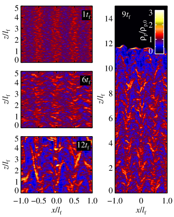
Figure 5: Sedimenting particles with a $k_{\rm x}=\pi/2$-mode in the particle density. We show different details (left) from a larger simulated domain (right), at different times ($t=1,6,9,12$ $t_{\rm f}$), based on runKH. We added initially noise in the particle velocity perturb the boundary between particle rich and poor. We believe that we see a “parasitic” Kelvin-Helmholtz instability appear over time.

3.4 Eggbox perturbation

Finally, we also perturb the system with an eggbox-like perturbation, in order to investigate the formation and evolution of particle swarms, which we will term particle droplets. The initial particle density perturbation is of the form

$$\rho_{\rm p}(x,z)=A\sin(k_{\rm x}x)\sin(k_{\rm z}z)\,,$$ (8)

with $A$ the amplitude of the two-dimensional perturbation. This initial condition can be inspected in Fig.6. The subsequent panels show the evolution of the inserted particle droplets. Initially they go through a phase of contraction without altering the amplitude. This can be seen in further detail in the vertical slices in Fig.7. The droplets remain in terminal velocity. Intriguingly, the wave steepening is scale-independent, as can be seen the right panel of Fig.7, where we have decreased the size of the droplets by a factor 2. Subsequently, the particle transforms in a characteristic mushroom cloud reminiscent of those seen in the standard Rayleigh-Taylor instability.

Figure 8 illustrates how non-linear drafting results in particle concentrations. Initially, the droplets concentrate the material by collapsing onto themselves. However, in the subsequent evolution it is clear that the overdense regions drag gas downwards with their sedimentation flow. Simultaneously, gas moves upwards in between the denser areas. This is an aspect of the unbalanced stratification that we discussed in Sec. 3.2.

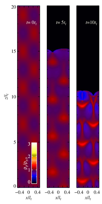
Figure 6: The evolution of particle droplets, at different times ($t=0,5,10$ $t_{\rm f}$), resulting in the emergence of characteristic Rayleigh-Taylor mushroom clouds. The colorbar give the color scale for the shown particle density. Results from runEGG.

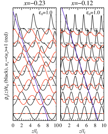
Figure 7: Slices through the evolution of the particle droplets, along the $z$-direction, similar to Fig.4. The droplets sediment at terminal velocity, and the wave steepening is independent of the initial droplet scale. The left panel shows run runEGG with $\lambda_{\rm x}=1,\lambda_{\rm z}=4$ and the right panel runEGG2 with $\lambda_{\rm x}=0.5,\lambda_{\rm z}=2$.

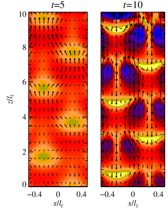
Figure 8: The particle and gas evolution around particle droplets, at times $t=5,10$ $t_{\rm f}$. Streamlines show the gas velocity, while the particle density is color coded as in Fig. 6. Results from runEGG.

3.5 Toy model of the drafting instability

The origin of the instability can be grasped from a simplified stability analysis, that is based on the observation that regions overdense in particles sediment faster than regions that are underdense in particles. Eq. (5) and Eq. (6) describe the behaviour of the particles, which only depends on the gas through the gas drag term. We now assume the gas velocity can be written as

$$u=\alpha(\epsilon-\epsilon_{0})v,$$ (9)

Here, $\alpha$ is a proportionality constant that can be determined numerically and which contains the dependence of the instability on the viscosity and the Mach number. The quantities $u$ and $v$ are the vertical gas and particle velocity. Effectively, we use that the linearised gas velocity $\delta u$ can be expressed proportional to the particle density perturbation $\delta u=\alpha(v_{\rm f}/\rho_{0})\delta\rho_{\rm p}$ (see Appendix B for more details). Physically, it expresses the observation that gas follows overdense particle regions, but locally momentum is conserved by the gas becoming buoyant and moving in the opposite direction in underdense regions.

This assumption allows us to reduce the equations to one dimension, even though the above approximation implicitly assumes two or three dimensions to be present to allow gas to move freely and not be trapped as in our stable one dimensional experiment (Fig.8). We will also approximate the gas density to be constant.

The equilibrium state corresponds to pure sedimentation with $\epsilon=\epsilon_{0}$ and the particles having the terminal velocity $v=-gt_{\rm f}$. The dispersion relation for Fourier modes of the form $\propto\exp\left(\omega t-ikx\right)$ becomes

$$\omega^{\prime}=+ik^{\prime}+\frac{1}{2}\left(-1\pm\sqrt{1-4\alpha\epsilon_{0}k^{\prime}i}\right)\,,$$ (10)

where $\omega^{\prime}$ is the growth amplitude, $k^{\prime}=2\pi/\lambda^{\prime}$ the wave number of wavelength $\lambda^{\prime}$ in friction units. The last term of Eq. (10) is always positive for $\epsilon_{0}>0$, resulting in the exponential growth of the instability. The fastest growing modes are those with the shortest wavelength. This result, although derived somewhat differently (see Appendix B), is identical to that of plate drag (Goodman & Pindor 2000; Chiang & Youdin 2010; Jacquet et al. 2011). The real part of the dispersion relation is illustrated in Fig. 12.

For large $k$, corresponding to short wavelengths ($\lambda\ll 8\pi\alpha\epsilon_{0}t_{f}^{2}g$), the growth rate can be approximated by

$$\omega^{\prime}_{\rm grow}\approx\frac{1}{\sqrt{2}}\sqrt{\alpha\epsilon_{0}k^{\prime}}\,,$$ (11)

by series expansion to leading order. Alternatively, we can express this result no longer in friction units but as

$$\omega_{\rm grow}\approx\sqrt{\alpha\pi\frac{\epsilon_{0}g}{\lambda}}\,.$$ (12)

Interestingly, in this asymptotic limit case the growth rate no longer depends on the particle size (or more accurately the friction time), but only on the spatial scale and the dust-to-gas ratio. On larger scales, the limit expression of the growth rate takes the form

$$\omega^{\prime}_{\rm grow}=\left(\alpha\epsilon_{0}k^{\prime}\right)^{2}\,,$$ (13)

to leading order. Therefore, the growth rate of the drafting instability rapidly decreases with increased spatial scale. In this branch the growth rate does depend on the particle size,

$$\omega_{\rm grow}=(\alpha\epsilon kg)^{2}t_{\rm f}^{3}\,.$$ (14)

3.6 Dependence on the Reynolds number

If the toy model is right, then the growth rate scales as $\omega^{\prime}_{\rm grow}\propto k^{{}^{\prime}2}$ on length scales above the characteristic scale

$$\lambda_{\rm knee}=2^{4/3}\pi\alpha\epsilon_{0}l_{\rm f},$$ (15)

obtained from balancing the fast and slow growth branches (Eq. 11 and 13).

Viscous damping has a similar quadratic dependence on $k^{\prime}$. Therefore a viscosity cut-off exists: at $\nu$ larger than $\nu_{\rm crit}$ growth of the instability is terminated. We find the critical viscosity by equating the large scale growth time scale (Eq. 13) with the viscous time scale ($\lambda^{\prime 2}/{\nu^{\prime}}$),

$$\nu_{\rm crit}^{\prime}=2\pi(\alpha\epsilon)^{2}\,.$$ (16)

The determination of $\alpha$ allows us to scale the growth rates of the toy model. From Fig. 9 we find numerically that above viscosities of around $\nu^{\prime}\sim 10^{-3}$, the instability does not show up. A critical viscosity of $\nu^{\prime}_{\rm crit}$$\sim$$10^{-3}$ would correspond to $\alpha\sim 10^{-2}$. Such an estimate is an approximate agreement with the seen correlation between particle density variations $\epsilon$ and the gas fluid velocity in Fig. 3.

For viscosities below the viscosity cut-off on the small scale branch, the the largest growing wavenumber scales as

$$k_{\rm crit}^{\prime}=\left(2\pi^{2}\frac{\alpha\epsilon_{0}}{\nu^{\prime 2}}\right)^{1/3}$$ (17)

by setting the viscous time scale equal to small scale growth rate (Eq. 11). Therefore the growth rate scales with the viscosity as $\omega^{\prime}\propto\nu^{\prime-1/3}$. This indeed agrees with the results shown in Fig. 9.

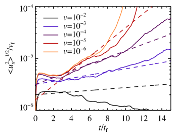
Figure 9: Viscosity dependency on the growth rate of the drafting instability. Dashed lines give the growth time scaling where $\omega\propto\nu^{-1/3}$, as in the toy model. At high viscosities over $\nu^{\prime}\approx 10^{-3}$ we no longer identify growth in the fluid velocity dispersion. Numerical results from runv2, runv3, run2, runv5, runv6.

3.7 Dependence on initial dust-to-gas ratio

The main free parameter in our model is the initial dust-to-gas ratio, also called the metallicity, when setting up the equilibrium stratification $\epsilon_{0}$. Evidently in the limit of negligible dust loading, we do not expect any dust clumping. We therefore study the dependency of the growth rate of the instability on lower than unity initial dust-to-gas ratio (Fig.10). To measure slower growth rates (and possibly the saturation of the instability), we need to extend the vertical domain, which we achieve by numerically scaling the system (runs run1-4.0.1, see Table 2).

We find that the instability does not vanish even at a 10 times reduced metallicity. The growth rate is slower, and there seems to be a longer dormant phase before particle concentrations settle in. The reason of this delay for the instability to kick in is unclear. Between $\epsilon_{0}=0.1$ to $\epsilon_{0}=1$ the growth rates scale approximately proportionally to $\sqrt{\epsilon_{0}}$, as expected form the toy model (Eq. 12).

At even lower metallicities, $\epsilon_{0}=0.05$ we do not recover the instability. Growth rates become too slow to identify any particle clumping in the simulation (run4.01).

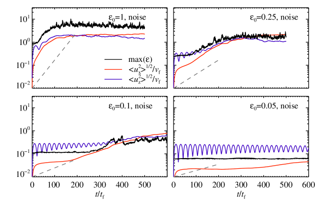
Figure 10: Long term evolution of the dust-to-gas ratio $\rm{max}(\epsilon)$ (black), combined with the horizontal $\sqrt{<u_{x}^{2}>}$ (red) and vertical $\sqrt{<u_{z}^{2}>}$ (blue). The grey dashed lines represent the growth rate scaling with $\sqrt{\epsilon_{0}}$, as found from the toy model (Eq. 11). The growth rate decreases with dust-to-gas ratio, and we are unable to measure growth rates below $\epsilon_{0}=0.05$. The small oscillations seen in vertical velocity dispersion for the low metallicity runs are the result of vertical waves which are due to a slight imbalance in the initial condition in elongated domains. The figure is based on the simulations run1.01,run2.01,run3.01,run4.01 (in order of decreasing metallicity).

4 Enhanced particle concentrations in protoplanetary discs

In this section, we rescale our simulation results to the context of the protoplanetary disc. Because the drafting effect seems to prefer higher dust-to-gas ratios than the percentage level initially expected in a protoplanetary disc, we will consider particle settling in a disc that has already undergone some grain growth, resulting in an already partly settled particle midplane (Sec. 4.1 and 4.2). In mass loaded regions, the swarms created by the drating instability may aid the formation of chondrules, which we explore in Sec. 4.3. Finally we comment on the relevance of the drafting instability in the possibly highly dust-enriched envelopes around protoplanets (Sec. 4.4).

4.1 Rescaling friction units

The friction units employed in our simulations can be readily rescaled to a protoplanetary disc setting, for a given particle size expressed in Stokes number

$$\tau_{\rm f}=t_{\rm f}\Omega_{\rm K},$$ (18)

where $\Omega_{\rm K}$ is the Keplerian frequency (for the definition of the friction time $t_{\rm f}$, see Eq. 3). From this definition, a time $t_{\rm f}$ corresponds to a fraction of a Keplerian time scale, $t_{\rm f}=\Omega_{\rm K}^{-1}\tau_{\rm f}$ . Similarly, the friction length $l_{\rm f}$ can be expressed as

$$l_{\rm f}=gt_{\rm f}^{2}=z\tau^{2}_{\rm f},$$ (19)

when the gravity is expressed as $\Omega^{2}z$. Here, $z$ is the height above the midplane. The friction length in the Minimum Mass Solar Nebula (MMSN, Hayashi 1981) at the top of a particle layer of thickness $H_{\rm p}$ can be written as

$$l_{\rm f}\approx 37\times 10^{3}\left(\frac{H_{\rm p}/H}{0.1}\right)\left(\frac{\tau_{\rm f}}{0.1}\right)^{2}\left(\frac{r}{5\,{\rm AU}}\right)^{5/4}\,{\rm km.}$$ (20)

This scale strongly depends on the particle size ($\tau_{\rm f}=0.1$ corresponds to a $2$ cm particle at an orbital distance of $r\approx 5$ AU). We have here assumed that the particle scale height is a constant fraction of the gas scale height $H$.

The ratio of the terminal velocity to the sound speed, the Mach number

$$Ma=\frac{v_{\rm f}}{c_{\rm s}}=0.01\left(\frac{H_{\rm p}/H}{0.1}\right)\left(\frac{\tau_{\rm f}}{0.1}\right),$$ (21)

reveals the incompressible nature of particle sedimentation.

We can ignore the overall rotation of the protoplanetary disc for the small scales that we consider here. The Rossby number $Ro=v_{\rm f}/(\Omega_{\rm K}l_{\rm f})$ takes the form: $Ro\sim 1/(\Omega_{\rm K}t_{\rm f})$, when using friction scales. Therefore, for particles with small Stokes number $\tau_{\rm f}=\Omega_{\rm K}t_{\rm f}\ll 1$, rotation is not important, and the rotation-free assumption is valid.

The kinematic molecular viscosity depends on the gas mean free path $\lambda$ in the midplane of the protoplanetary disc as

$$\nu=\frac{1}{2}c_{\rm s}\lambda\,.$$ (22)

The viscosity can then be expressed in friction units as

$$\frac{\nu}{g^{2}t_{\rm f}^{3}}=1.6\times 10^{-6}\left(\frac{H_{\rm p}/H}{0.1}\right)^{-2}\left(\frac{\tau_{\rm f}}{0.1}\right)^{-3}\left(\frac{r}{5\,{\rm AU}}\right)^{3/2}\,.$$ (23)

This value does not differ greatly from the nominal value probed in our numerical work [$\nu/(g^{2}t_{\rm f}^{3})=10^{-4}$, see also the list of simulations in Table 1]. The strong scaling with orbital radius becomes much weaker if one considers particles of constant radius, as opposed to constant Stokes number.

Finally, we also verify the viscous particle coupling criterion, given by Eq. (4), holds in the MMSN,

$$\frac{t_{\nu{\rm,pair}}}{t_{\rm f}}\approx 3.0\times 10^{-4}\left(\frac{\epsilon_{0}}{0.1}\right)^{-2/3}\left(\frac{\tau_{\rm f}}{0.1}\right)\left(\frac{r}{5\,{\rm AU}}\right)^{-31/6},$$ (24)

where $\epsilon_{0}$ is the approximate mean dust-to-gas ratio in the particle midplane.

4.2 Applying the toy model

With the help of the toy model we can attempt to further constrain where in the protoplanetary disc the drafting instability can occur. Because growth rates decrease rapidly at large scales, we only expect the instability to take place on the small scale branch, below the characteristic scale $\lambda_{\rm knee}$. From Eq. 15, we get

$$\lambda_{\rm knee} \approx 290\left(\frac{\alpha}{0.01}\right)\left(\frac{\epsilon_{0}}{0.1}\right)\left(\frac{H_{\rm p}/H}{0.1}\right)\left(\frac{\tau_{\rm f}}{0.1}\right)^{2}\left(\frac{r}{5\,{\rm AU}}\right)^{5/4}\,{\rm km}.$$ (25)

The dust-to-gas ratio of $\epsilon_{0}=0.1$ will be relevant in a midplane layer of solids with $H_{p}/H=0.1$, when the overall metallicity of the protoplanetary disc is the canonical $Z=0.01$. However, we have chosen to keep dust-to-gas ratio $\epsilon_{0}$ and the height of the particle layer $H_{\rm p}$ as independent quantities, because we do not necessarily want to study the conditions of a particle layer settled to equilibrium.

A lower limit on the scale of the instability is set by viscous damping of the instability at scales below the knee,

$$\lambda_{\rm visc}= \left(\frac{2^{2}\pi}{\alpha\epsilon_{0}}\right)^{1/3}\left(\frac{\nu}{g^{2}t_{\rm f}^{3}}\right)^{2/3}l_{\rm f}$$

$$\approx 93\left(\frac{\alpha}{0.01}\right)^{-1/3}\left(\frac{\epsilon_{0}}{0.1}\right)^{-1/3}\left(\frac{H_{\rm p}/H}{0.1}\right)^{-1/3}\left(\frac{r}{5\,{\rm AU}}\right)^{9/4}\,{\rm km.}$$ (26)

Note this scale, as opposed to the friction length $l_{\rm f}$ (Eq. 20), does not depend on the particle size.

In Fig. 11 we have illustrated the different relevant scales presented in Eq. (20), (25) and (26), as function of orbital radius. The instability would operate on a scale of the order of $10^{4}$ km in the outer parts of the protoplanetary disc for particles of cm in size, assuming a MMSN model. Note that Fig. 11 shows the scaling for an assumed constant particle size, as opposed to Eq. (20–26) that assume constant Stokes number.

4.3 Chondrules

Chondrules are mm-sized inclusions found in primitive meteorites originating from the asteroid belt. It is generally accepted that a chondrule is the product of a flash heating event. The exact nature of chondrule precursors is unknown. However the heating events likely occurred in particle swarms at least $100$ to $1000$ km wide, with a local number density of about $\sim$10 m^-3. In this way the loss of light isotopes (isotopic fractionation) is prevented by exchanging vapour from chondrule to chondrule (Cuzzi & Alexander 2006). This scenario requires local chondrule densities more than 100 times above a dust-to-gas ratio of unity. Even higher concentrations might be necessary to explain the retention of sodium (Alexander et al. 2008).

Such high chondrule densities are surprising, since small particles are hard to concentrate to the midplane. Even in the absence of other forms of turbulence, particles sediment to a midplane with dust-to-gas ratio not higher than approximately unity, because of the stirring caused by the streaming instability (Bai & Stone 2010a). However, the isotopic constraints on the need to concentrate chondrules weaken if the gas at the chondrule formation sites had a non-solar composition. The atmospheres around planetary embryos have been proposed to be such locations (Morris et al. 2012). Nevertheless, in this scenario, pre-clumping of solids by a factor of at least $10$ over midplane densities remains necessary and the shock waves invoked to melt chondrules lead in fact to destructive collisions (Jacquet & Thompson 2014).

Small particles are difficult to concentrate in the inner protoplanetary disc, because of the strong sensitivity of the preferential scale of the instability on particle size (Eq. 20 and Eq. 25), as can be seen in Fig. 11. Nevertheless the connection to chondrule formation is tantalizing, especially because if clumping conditions are met, the drafting effect only weakly depends on particle size and efficiently clusters particles down to very small sizes (Eq. 12). This is different from, for example, the streaming instability that has a preferred particle size, somewhat above that of chondrules for nominal metallicities (Carrera et al. 2015).

The drafting instability could operate on such small scales, if some form of pre-concentration of solids would occur. Possibly such enhanced particle densities could occur near the Kolmogorov scale of the disc turbulence (Cuzzi et al. 2001). Alternatively, near sublimation lines particle concentrations can dramatically peak (Ros & Johansen 2013). An increase in the dust-to-gas ratio can also occur by accretion of gas onto the star, which depletes the disc relative to the MMSN (Bitsch et al. 2015). Alternatively, growth rates could be increased if the unknown chondrule precursors are much larger than the chondrules they are turned into after the heating event. Even so, it remains to be seen if drafting instabilities can push particle concentrations to the desired high levels, even in such favourable instances.

4.4 Planetary atmospheres

The drafting instability might be important in the atmospheres of giant planets. The opacity in the outer envelope, which regulates the transport of heat, comes from the dust component. Under standardly assumed opacities, it is difficult to cool the envelope and trigger runaway gas accretion (Ikoma et al. 2000; Piso & Youdin 2014). However, clumping of solids and the growth of the accreted dust could significantly reduce the opacity in the upper atmosphere. The friction length for particles sedimenting in a planetary atmosphere is given by

$$l_{\rm f,plan} =\frac{GM}{r_{\rm B}^{2}}t_{\rm f}^{2}$$

$$\approx 7.2\times 10^{3}\left(\frac{R}{1\,{\rm mm}}\right)^{2}\left(\frac{M}{5\,{\rm M}_{\rm E}}\right)^{-1}\left(\frac{r}{5\,{\rm AU}}\right)^{5}\,{\rm km}\,,$$ (27)

where $r_{\rm B}=GM/c_{\rm s}^{2}$ is the thermal Bondi radius of a planet with mass $M$, corresponding to the outer edge of the atmosphere. We have here considered particles on top of the envelope, but deeper in the planet the friction time shrinks due to the increase in density. Applying the toy model, we estimate the knee scale in the upper envelope at

$$\lambda_{\rm knee,plan}\approx 570\left(\frac{\alpha}{0.01}\right)\left(\frac{\epsilon_{0}}{1}\right)\left(\frac{R}{1\,{\rm mm}}\right)^{2}\left(\frac{M}{5\,{\rm M}_{\rm E}}\right)^{-1}\left(\frac{r}{5\,{\rm AU}}\right)^{5}\,{\rm km}\,,$$ (28)

which is above the damping viscosity scale at

$$\lambda_{\rm visc,plan}\approx 13\left(\frac{\alpha}{0.01}\right)^{-1/3}\left(\frac{\epsilon_{0}}{1}\right)^{-1/3}\left(\frac{M}{5\,{\rm M}_{\rm E}}\right)^{1/3}\left(\frac{r}{5\,{\rm AU}}\right)^{2}\,{\rm km.}$$ (29)

The formation of ice giants and super-Earths might be paired with significant amounts of dust in their low-mass gaseous envelopes (Lee et al. 2014). These scaling relations argue that order-of-unity mass loading of atmospheres will lead to clumping and the breakup of the dust component, providing an upper limit on the dust opacity.

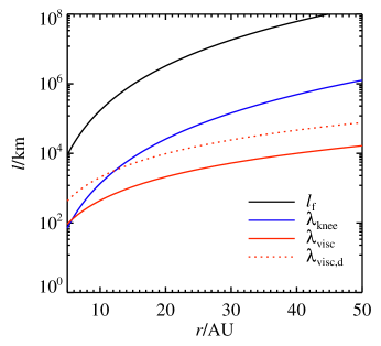
Figure 11: Relevant length scales for the drafting instability in the Minimum Mass Solar Nebula: the friction length ($l_{\rm f}$), the upper scale for fast growth ($\lambda_{\rm knee}$), and the scale at which viscosity dominates ($\lambda_{\rm visc}$). We consider particles located at a particle scale height above the midplane, with $H_{\rm p}/H=0.1$ and the midplane dust-to-gas ratio is $0.1$. We take the toy model parameter to be $\alpha=0.01$. Particles are assumed to be $1$ cm in radius, or $1$ mm in a gas depleted disc with 10 times lower gas surface density (in that case the curves remain the same, but viscous scale $\lambda_{\rm visc,d}$ is now the red dotted line). Likely the instability does not operate in the inner ($<5$ AU) of the protoplanetary disc, unless particles are large or significant pre-concentration occurs.

5 Future outlook

5.1 Laboratory Experiments

This study supports ongoing work to investigate drag instabilities in the laboratory. A full description of the apparatus constructed at the Max Planck Institute for Dynamics and Self-Organisation and first results will be presented in an accompanying paper (Capelo et al, 2016, in prep). Here, we restrict ourselves to highlight some aspects relevant to the understanding of the numerical results presented in this paper.

The experimental apparatus consists of a cylindrical vessel, housing a gas stream operating at pressures in the range of $0.5-10^{3}$ millibar. The axial component of the cylindrical flow is parallel with the direction of Earth’s gravity, similar to the sedimentation configuration in the simulations presented here. The upwards steady-state flow will be seeded with weakly inertial particles, with typical sizes of $20$-$90$ $\mu$m. The range of operational pressures and temperatures, listed in Table 3, will then allow us to span both the Stokes and Epstein drag regimes.

The particle entrainment happens upstream in the fluid flow. There the system is in a brief transient state. The solids are transported and mixed with the gas by the time the flow reaches the steady-state conditions in which the measurements are to be made. This is done to make a fair comparison with the nearly homogeneously mixed initial conditions of the two-fluid dust/gas models.

Table 3 summarises the parameter region in which the experiment operates, including gas state variables, Mach and Reynolds numbers. The flow conditions are incompressible and laminar. The experiment will be the first in its kind probing the Epstein drag regime in a fluid with equal mass loading of gas and particles.

The experiment described here is somewhat analogous to particle suspension experiments in Newtonian fluids with low particle Reynolds number (Guazzelli & Hinch 2011). However, in these studies volume fractions, $\phi=n_{\rm p}R^{3}$ (with $n_{\rm p}$ and $R$ the particle number density and radius), are no lower than $\phi\approx 0.01\%$. Our experiment operates at $\phi\approx 10^{-4}\%$, when the dust-to-gas ratio is unity, for solid spherical particles with densities ranging from that of vitreous carbon ($\rho_{\bullet}$=1.4 g cm^-3) to steel ($\rho_{\bullet}$=8 g cm^-3). The low particle Reynolds number, $Re_{\rm p}$, in such suspension experiments comes from the use of a fluid with high dynamic viscosity. The particles are very buoyant and slowly creep through a thick liquid. Here, on the other hand, the low values of $Re_{\rm p}$ come from the fact that the kinematic viscosity becomes high when the gas density is low. It is encouraging that such experiments, even if in a regime different from the one studied here, show interesting particle dynamics (Batchelor 1972), such as particle Rayleigh-Taylor mushrooms and drafting particle trains (Pignatel et al. 2009; Matas et al. 2004).

Table 3: Parameters of the laboratory experiment. The range of pressure values correspond to different settings used to seed particles of various sizes and densities in the flow. The range in temperature values corresponds to the cooling that occurs as the gas expands to reach steady low-pressure conditions. The Reynolds numbers are calculated using the definition, $Re=\rho vL/\mu$, where $\rho$ is the density of the gas, $v$ the characteristic velocity, $L$ the characteristic length scale, and $\mu_{\rm air}=1.8\times 10^{-5}$ kg m^-1 s^-1 is the dynamic viscosity of air at room temperature. For the particle Reynolds number, we take the characteristic velocity and size to be the terminal velocity and the particle diameters, respectively. The density of the gas is estimated using the measured values of temperature and pressure, assuming a mean molar mass of air $M_{\rm air}=0.02891$ kg mol^-1 and molar gas constant $R=8.314$ m³ Pa K^-1 mol^-1. The global Reynolds number comes from the mean flow velocity and the tube diameter. Similarly, the Mach number is the ratio of the mean flow velocity to the sound speed at the measured temperature, again assuming the same values of $R$ and $M_{\rm air}$.

Property	Value
Working gas	air
Tube height	1.6 m
Tube diameter	9 cm
Friction time	0.05-0.08 s
Friction length	$\approx$ 3-7 cm
Pressure range	10-8000 Pa
Temperature	16-22∘C
Estimated mean flow speed	1.2 m s-1
Global Reynolds number	0.6 - 6
Particle Reynolds number	0.009-0.08
Mach number	0.003
Solid-to-gas ratio	$0.1$–$10$

Time-resolved data on the particle trajectories will be obtained from high-resolution cameras and 3-dimensional Lagrangian particle tracking (Xu 2008; Ouellette et al. 2006). This is a common technique to study both tracer and intertial particles in fluids. The typical measured and derived quantities are the probability density distributions of the particle velocities and accelerations, their statistical moments, and correlation and structure functions.

The obtained data will provide an interesting comparison to the results shown in this paper. The parameter regime is sufficiently similar to the numerical experiments that we expect the drafting instability to manifest itself. Particle tracking would not only allow the detection of particle swarms, but also the individual particle dynamics. For instance, Fig. 2 demonstrates that the growing maximum in particle velocity dispersion traces the increase in maximum particle density. Such statistical measurements of the particles will allow qualitative comparison between the numerical work and the experiments.

5.2 Numerical work

We have here presented several numeric experiments to demonstrate a drafting instability. Future work will refine the estimates made in this paper.

For example, currently the numerical set up is limited to studying sedimentation on rather short timescales, set by the length of the simulation domain. This could be avoided in future work by implementing a form of periodic boundary conditions in the vertical direction, which would recycle particles.

To aid the interpretation of the experimental results, it will be necessary to specifically reproduce the parameter regime in which the apparatus operates. Additionally, refined boundary conditions will be needed to approximate the experimental set-up. Such work is under progress, but evidently awaits the first experiments.

We have also argued that the drafting instability could be of relevance in a protoplanetary disc. To study this connection in more detail, it will be necessary to simulate numerically expensive larger domains encompassing the disc midplane. Additionally, the connection between the drafting and streaming instability could be studied in more detail. Ultimately, the results should be placed in the context of other sources of disc turbulence, such as the magnetorotational instability operating in sufficiently ionised regions or in the penetration of vertical shear instability to the midplane (Turner et al. 2014). Additionally, the growth of particles through coagulation or condensation will need to be taken into account in a self-consistent matter. Future work is needed to understand the possibly constructive interplay of these mechanisms.

6 Summary

In this paper we have demonstrated the presence of a drafting instability when particles sediment through a fluid in hydrostatic balance. On time scales of tens of friction times particle unmix out of a homogeneous mixture and particle concentrations increase by a factor $10$.

The presence of such an instability was not expected because it evades detection in an analytic linear stability analysis. However, our numerical results demonstrate that the system is non-linearly unstable. The exact nature of the instability is difficult to determine. We interpret the instability to be the result of an imbalance in the stratification locally disturbing the hydrostatic balance. We support this hypothesis with a simple toy model that captures some of the main characteristics of the instability. Growth is fastest at the smallest available scales, increases with the square root of the dust-to-gas ratio and a critical scale is identified at which viscosity overwhelms the instability.

By expressing our numerical results in a system of friction units, we can exploit our results by scaling them to either upcoming laboratory experiments or the protoplanetary disc. We argue that an experiment can probe a similar regime with dust-to-gas ratio around unity that is of interest here. In protoplanetary discs the drafting instability may take place in particle-rich layers above the midplane in the outer regions of the disc, on scales smaller than previously studied. In these regions where the conditions for the drafting instability are met, we have shown that sedimenting particles spontaneously form dense clumps. Future work will be needed to investigate to what degree this clumping affects coagulation rates and whether the drafting instability can create the dense environment necessary for chondrule flash heating.

Appendix A Linear stability analysis

We briefly rederive the stability analysis for a particle gas-mixture in a non-rotating flow (Youdin & Goodman 2005; Jacquet et al. 2011). We demonstrate the result in two spatial dimensions, but our conclusions remain valid when generalized to three dimensions.

A.1 Governing equations

We assume the gas to be incompressible, in line with Youdin & Goodman (2005),

$$\frac{\partial u_{x}}{\partial x}+\frac{\partial u_{z}}{\partial z}=0,$$ (30)

and use the standard momentum equations

$$\frac{\partial u_{x}}{\partial t}+u_{x}\frac{\partial u_{x}}{\partial x}+u_{z}\frac{\partial u_{x}}{\partial z} =-\frac{1}{\rho}\frac{\partial P}{\partial x}+\frac{1}{t_{\rm f}}\frac{\rho_{\rm p}}{\rho}\left(v_{x}-u_{x}\right)\,,$$ (31)

$$\frac{\partial u_{z}}{\partial t}+u_{x}\frac{\partial u_{z}}{\partial x}+u_{z}\frac{\partial u_{z}}{\partial z} =-g-\frac{1}{\rho}\frac{\partial P}{\partial z}+\frac{1}{t_{\rm f}}\frac{\rho_{\rm p}}{\rho}\left(v_{z}-u_{z}\right).$$ (32)

Similarly, for the particle fluid we make use of the continuity equation,

$$\frac{\partial\rho_{\rm p}}{\partial t}+\frac{\partial}{\partial x}\left(\rho_{\rm p}v_{x}\right)+\frac{\partial}{\partial z}\left(\rho_{\rm p}v_{z}\right)=0,$$ (33)

and the set of momentum equations

$$\frac{\partial v_{x}}{\partial t}+v_{x}\frac{\partial v_{x}}{\partial x}+v_{z}\frac{\partial v_{x}}{\partial z} =-\frac{1}{t_{\rm f}}\left(v_{x}-u_{x}\right)\,,$$ (34)

$$\frac{\partial v_{z}}{\partial t}+v_{x}\frac{\partial v_{z}}{\partial x}+v_{z}\frac{\partial v_{z}}{\partial z} =-g-\frac{1}{t_{\rm f}}\left(v_{z}-u_{z}\right).$$ (35)

This completes the model with 6 parameters ($\rho_{\rm p},\rho,v_{x},v_{z},u_{x},u_{z}$), and as many equations.

A.2 Equilibrium solution

In equilibrium we have no vertical motion $(u_{x}=0,v_{x}=0)$. Additionally, we assume the gas to be in the rest frame, $u_{z}=0$, and particles to be initially uniformly spread ($\rho_{\rm p}=\rho_{\rm p,0}$ constant). This leaves the particle continuity and $z$-momentum equations as the non-trivial equations determining $v_{z}$ and $\rho,\rho_{\rm p}$,

$$\frac{\partial}{\partial z}\left(\rho_{\rm p}v_{z}\right) =0\,,$$ (36)

$$v_{z}\frac{\partial v_{z}}{\partial z} =-g-\frac{1}{t_{\rm f}}v_{z}\,,$$ (37)

$$0 =-g-\frac{c_{\rm s}^{2}}{\rho}\frac{\partial\rho}{\partial z}+\frac{1}{t_{\rm f}}\frac{\rho_{\rm p}}{\rho}v_{z}.$$ (38)

In the last equation we have assumed an isothermal gas, $P=\rho c_{\rm s}^{2}$. The equilibrium solution then takes the form

$$v_{z} =-gt_{\rm f}\,,$$ (39)

$$\rho =\left(\rho_{\rm p}+\rho_{\rm b}\right)\exp\left(-\frac{g}{c_{\rm s}^{2}}z\right)-\rho_{\rm p},$$ (40)

where $\rho_{\rm b}$ is the gas density at the $z=0$ boundary.

A.3 Dispersion relation

We now consider a first order perturbation of this equilibrium state. For the gas we find

$$\frac{\partial u_{x}^{\prime}}{\partial x}+\frac{\partial u_{z}^{\prime}}{\partial z} =0\,,$$ (41)

$$\frac{\partial u_{x}^{\prime}}{\partial t} =-\frac{c_{\rm s}^{2}}{\rho_{0}}\frac{\partial\rho^{\prime}}{\partial x}+\frac{1}{t_{\rm f}}\frac{\rho_{\rm p,0}}{\rho_{0}}\left(v_{x}^{\prime}-u_{x}^{\prime}\right)\,,$$ (42)

$$\frac{\partial u_{z}^{\prime}}{\partial t} =-\frac{c_{\rm s}^{2}}{\rho_{0}}\frac{\partial\rho^{\prime}}{\partial z}-\frac{g}{\rho_{0}}\rho^{\prime}-\frac{g}{\rho_{0}}\rho_{p}^{\prime}+\frac{1}{t_{\rm f}}\frac{\rho_{\rm p,0}}{\rho_{0}}\left(v_{z}^{\prime}-u_{z}^{\prime}\right).$$ (43)

For the particles we get

$$\frac{\partial\rho_{\rm p}^{\prime}}{\partial t}+\rho_{\rm p,0}\frac{\partial v_{x}^{\prime}}{\partial x}+\rho_{\rm p,0}\frac{\partial v_{z}^{\prime}}{\partial z}+v_{z,0}\frac{\partial\rho_{\rm p}^{\prime}}{\partial z} =0\,,$$ (44)

$$\frac{\partial v_{x}^{\prime}}{\partial t}+v_{z,0}\frac{\partial v_{x}^{\prime}}{\partial z} =-\frac{1}{t_{\rm f}}\left(v_{x}^{\prime}-u_{x}^{\prime}\right)\,,$$ (45)

$$\frac{\partial v_{z}^{\prime}}{\partial t}+v_{z,0}\frac{\partial v_{z}^{\prime}}{\partial z} =-\frac{1}{t_{\rm f}}\left(v_{z}^{\prime}-u_{z}^{\prime}\right).$$ (46)

For modes of the form $A^{\prime}\propto\exp(\omega t-ik_{x}-ik_{z})$, we find that the system only has non-zero solutions when the determinant is zero,

$$\left(\omega-iv_{z}k_{z}\right)\left(\omega-iv_{z}k_{z}+t_{\rm f}^{-1}\right)\\ \left(\omega^{2}+\left((1+\epsilon)t_{\rm f}^{-1}-ik_{z}v_{z,0}\right)\omega-\epsilon t_{\rm f}^{-1}ik_{z}v_{z,0}\right)=0\,.$$ (47)

The first term represents a pure particle mode falling at the terminal velocity, while the second term represents particle motion damped by gas drag. The last factor of this expression has the solutions

$$\omega =\frac{v_{z}k_{z}}{2}i+\frac{(1+\epsilon)t_{\rm f}^{-1}}{2}\left(-1\pm\sqrt{1-\frac{k_{z}^{2}v_{z,0}^{2}t_{\rm f}^{2}}{(1+\epsilon)^{2}}+2\frac{(\epsilon-1)k_{z}v_{z,0}t_{\rm f}}{(1+\epsilon)^{2}}i}\right).$$ (48)

The real part of the square root term is always below unity (${\rm Re}\left(\sqrt{1-ix}\right)<1$ for any $x$), so the perturbation is damped.

In summary, this analysis shows that there are no growing modes under the assumption of incompressibility. Possibly, unstable modes could be found when relaxing the assumption of incompressibility, or by using more realistic equations of state or by exploring non-local perturbation techniques. We leave this for future work, given the complexity of such investigations.

Appendix B Toy model dispersion relation

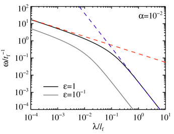
Figure 12: Linear behaviour of the toy model. In black, the real solution to the dispersion relation is given (Eq. 10, with $\alpha=0.01$). The knee, the largest scale for fast growth, is located at $\lambda_{\rm knee}\approx 0.08$. The gray curve is the result for a dust-to-gas ratio of $0.1$ as opposed to unity. The dashed red line gives the high $k$ approximation (Eq. 11) and the dashed blue line gives the low $k$ approximation (Eq. 13).

We start with making the ansatz that

$$u=\alpha(\epsilon-\epsilon_{0})v\,,$$ (49)

which removes the explicit dependency on the equations for the gas component. Here $\alpha$ is a proportionality parameter that encapsulates the viscosity dependency and remains to be determined through numerical simulations. We also, for simplicity, assume a constant gas density, $\rho=\rho_{0}$. Subsequently, the drag term in the particle momentum equation takes the form

$$-\frac{1}{t_{\rm f}}\left(v-u\right)=-\frac{v}{t_{\rm f}}\left[1-\alpha(\epsilon-\epsilon_{0})\right]\,.$$ (50)

In equilibrium, the dust-to-gas ratio, $\epsilon=\rho_{\rm p}/\rho$, is constant. The momentum equation then shows that particles move, as desired, with terminal velocity,

$$v_{0} =-gt_{\rm f}\,.$$ (51)

We now linearize the system of particle equations

$$\partial_{t}\rho_{\rm p}^{\prime}+\rho_{\rm p,0}\partial_{z}v^{\prime}+v_{0}\partial_{z}\rho_{\rm p}^{\prime} =0\,,$$ (52)

$$\partial_{t}v^{\prime}+v_{0}\partial_{z}v^{\prime} =-g-\frac{v_{0}+v^{\prime}}{t_{\rm f}}(1-\alpha\epsilon^{\prime})\,.$$ (53)

The last two terms simplify to

$$-g-\frac{v_{0}+v^{\prime}}{t_{\rm f}}(1-\alpha\epsilon^{\prime}) =-\frac{v^{\prime}}{t_{\rm f}}-g\alpha\frac{\rho_{\rm p}^{\prime}}{\rho_{0}}\,.$$ (54)

Taking now modes of the form $A^{\prime}\propto\exp\left(\omega t-ikz\right)$ we are left with the following system of equations

$$\begin{pmatrix}\omega-ikv_{0}&-ik\rho_{\rm p,0}\\ \alpha\frac{g}{\rho_{0}}&\omega-ikv_{0}+\frac{1}{t_{\rm f}}\end{pmatrix}\begin{pmatrix}\rho_{\rm p}^{\prime}\\ v^{\prime}\end{pmatrix}=\begin{pmatrix}0\\ 0\end{pmatrix}.$$ (55)

Non-zero solutions are found when

$$\beta^{2}+\frac{\beta}{t_{\rm f}}+i\alpha\epsilon_{0}gk=0,$$ (56)

where $\beta=\omega-ikv_{0}$. Thus we find

$$\beta=\frac{1}{2t_{\rm f}}\left(-1\pm\sqrt{1-4\alpha\epsilon_{0}gt_{\rm f}^{2}ki}\right)$$ (57)

where the last term has a positive real part larger than $1$, for any product $\alpha\epsilon_{0}gt_{\rm f}^{2}$ different from $0$. This reproduces Eq. (10), allowing the approximation of the two limit cases, Eq. (11) at small scales and Eq. (13) at large scales. The shape of the dispersion relation and the two limit cases can be inspected in Fig. 12.

Appendix C Particle number test

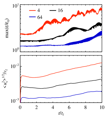
Figure 13: Evolution of the maximal particle density (top) and the horizontal gas dispersion (bottom), for 4, 16, and 32 particles per gridcell (respectively red, black, and blue curves). The initial maximal particle overdensity is reduced from $\epsilon/\epsilon_{0}=2.4$ to $1.6$ and finally $1.3$, when increasing the particle number by a factor of $4$ each time. The lowest particle number simulation shows fastest growth. In higher particle number runs the initial dormant phase persists longer and growth rates become lower. Results from run2.n4, run2, run2.n64.

Particle numbers of 16 superparticles per gridcell are sufficient to capture correctly the evolution of the particle–gas mixture. However, increased particle numbers decrease the noise amplitude that is initially injected. In Fig. 13 we show the evolution of the maximal particle density and gas velocity dispersion, as function of the particle number. Because of the non-linear nature of the drafting instability one can see that the decreased noise amplitude with increased particle number prolongs a dormant state before the instability comes fully into effect and growth rates decrease moderately. However, if one ignores the protracted dormant phase, growth rates between $16$ (our nominal value) and $64$ particles per gridcells are undistinguishable, although slower than the $4$ particles per gridcell case.

References

- Alexander et al. (2008) Alexander, C. M. O. ., Grossman, J. N., Ebel, D. S., & Ciesla, F. J. 2008, Science, 320, 1617
- Bai & Stone (2010a) Bai, X.-N. & Stone, J. M. 2010a, ApJ, 722, 1437
- Bai & Stone (2010b) Bai, X.-N. & Stone, J. M. 2010b, ApJS, 190, 297
- Bai & Stone (2010c) Bai, X.-N. & Stone, J. M. 2010c, ApJ, 722, L220
- Batchelor (1972) Batchelor, G. K. 1972, Journal of Fluid Mechanics, 52, 245
- Birnstiel et al. (2012) Birnstiel, T., Klahr, H., & Ercolano, B. 2012, A&A, 539, A148
- Bitsch et al. (2015) Bitsch, B., Johansen, A., Lambrechts, M., & Morbidelli, A. 2015, A&A, 575, A28
- Brandenburg (2003) Brandenburg, A. 2003, Computational aspects of astrophysical MHD and turbulence, ed. A. Ferriz-Mas & M. Núñez, 269
- Brandenburg & Dobler (2002) Brandenburg, A. & Dobler, W. 2002, Computer Physics Communications, 147, 471
- Brauer et al. (2008) Brauer, F., Dullemond, C. P., & Henning, T. 2008, A&A, 480, 859
- Carrera et al. (2015) Carrera, D., Johansen, A., & Davies, M. B. 2015, ArXiv e-prints
- Chiang & Youdin (2010) Chiang, E. & Youdin, A. N. 2010, Annual Review of Earth and Planetary Sciences, 38, 493
- Cuzzi & Alexander (2006) Cuzzi, J. N. & Alexander, C. M. O. 2006, Nature, 441, 483
- Cuzzi et al. (2001) Cuzzi, J. N., Hogan, R. C., Paque, J. M., & Dobrovolskis, A. R. 2001, ApJ, 546, 496
- Drazin & Reid (2004) Drazin, P. G. & Reid, W. H. 2004, Hydrodynamic Stability
- Dra̧żkowska & Dullemond (2014) Dra̧żkowska, J. & Dullemond, C. P. 2014, A&A, 572, A78
- Epstein (1924) Epstein, P. S. 1924, Physical Review, 23, 710
- Goodman & Pindor (2000) Goodman, J. & Pindor, B. 2000, Icarus, 148, 537
- Guazzelli & Hinch (2011) Guazzelli, É. & Hinch, J. 2011, Annual Review of Fluid Mechanics, 43, 97
- Guillot et al. (2014) Guillot, T., Ida, S., & Ormel, C. W. 2014, A&A, 572, A72
- Haugen & Brandenburg (2004) Haugen, N. E. L. & Brandenburg, A. 2004, Phys. Rev. E, 70, 026405
- Hayashi (1981) Hayashi, C. 1981, Progress of Theoretical Physics Supplement, 70, 35
- Hendrix & Keppens (2014) Hendrix, T. & Keppens, R. 2014, A&A, 562, A114
- Ikoma et al. (2000) Ikoma, M., Nakazawa, K., & Emori, H. 2000, ApJ, 537, 1013
- Jacquet et al. (2011) Jacquet, E., Balbus, S., & Latter, H. 2011, MNRAS, 415, 3591
- Jacquet & Thompson (2014) Jacquet, E. & Thompson, C. 2014, ApJ, 797, 30
- Johansen et al. (2014) Johansen, A., Blum, J., Tanaka, H., et al. 2014, Protostars and Planets VI, 547
- Johansen et al. (2011) Johansen, A., Klahr, H., & Henning, T. 2011, A&A, 529, A62
- Johansen et al. (2007) Johansen, A., Oishi, J. S., Mac Low, M.-M., et al. 2007, Nature, 448, 1022
- Johansen & Youdin (2007) Johansen, A. & Youdin, A. 2007, ApJ, 662, 627
- Johansen et al. (2009) Johansen, A., Youdin, A., & Mac Low, M.-M. 2009, ApJ, 704, L75
- Johansen et al. (2012) Johansen, A., Youdin, A. N., & Lithwick, Y. 2012, A&A, 537, A125
- Kataoka et al. (2013) Kataoka, A., Tanaka, H., Okuzumi, S., & Wada, K. 2013, A&A, 557, L4
- Kowalik et al. (2013) Kowalik, K., Hanasz, M., Wóltański, D., & Gawryszczak, A. 2013, MNRAS, 434, 1460
- Krijt et al. (2015) Krijt, S., Ormel, C. W., Dominik, C., & Tielens, A. G. G. M. 2015, A&A, 574, A83
- Lambrechts & Johansen (2012) Lambrechts, M. & Johansen, A. 2012, A&A, 544, A32
- Lambrechts & Johansen (2014) Lambrechts, M. & Johansen, A. 2014, A&A, 572, A107
- Lee et al. (2014) Lee, E. J., Chiang, E., & Ormel, C. W. 2014, ApJ, 797, 95
- Lyra & Kuchner (2013) Lyra, W. & Kuchner, M. 2013, Nature, 499, 184
- Matas et al. (2004) Matas, J.-P., Glezer, V., Guazzelli, É., & Morris, J. F. 2004, Physics of Fluids, 16, 4192
- Miniati (2010) Miniati, F. 2010, Journal of Computational Physics, 229, 3916
- Morris et al. (2012) Morris, M. A., Boley, A. C., Desch, S. J., & Athanassiadou, T. 2012, ApJ, 752, 27
- Ouellette et al. (2006) Ouellette, N., Xu, H., & Bodenschatz, E. 2006, Experiments in Fluids, 40, 301
- Pignatel et al. (2009) Pignatel, F., Nicolas, M., Guazzelli, É., & Saintillan, D. 2009, Physics of Fluids, 21, 123303
- Piso & Youdin (2014) Piso, A.-M. A. & Youdin, A. N. 2014, ApJ, 786, 21
- Raettig et al. (2015) Raettig, N., Klahr, H., & Lyra, W. 2015, ArXiv e-prints
- Ros & Johansen (2013) Ros, K. & Johansen, A. 2013, A&A, 552, A137
- Turner et al. (2014) Turner, N. J., Fromang, S., Gammie, C., et al. 2014, Protostars and Planets VI, 411
- Weidenschilling (1977) Weidenschilling, S. J. 1977, MNRAS, 180, 57
- Weidenschilling (2006) Weidenschilling, S. J. 2006, Icarus, 181, 572
- Xu (2008) Xu, H. 2008, Measurement Science and Technology
- Yang & Johansen (2014) Yang, C.-C. & Johansen, A. 2014, ApJ, 792, 86
- Youdin & Johansen (2007) Youdin, A. & Johansen, A. 2007, ApJ, 662, 613
- Youdin & Chiang (2004) Youdin, A. N. & Chiang, E. I. 2004, ApJ, 601, 1109
- Youdin & Goodman (2005) Youdin, A. N. & Goodman, J. 2005, ApJ, 620, 459
- Youdin & Lithwick (2007) Youdin, A. N. & Lithwick, Y. 2007, Icarus, 192, 588