Isotope effect on gyro-fluid edge turbulence and zonal flows

Abstract

The role of ion polarisation and finite Larmor radius on the isotope effect on turbulent tokamak edge transport and flows is investigated by means of local electromagnetic multi-species gyro-fluid computations. Transport is found to be reduced with the effective plasma mass for protium, deuterium and tritium mixtures. This isotope effect is found for both cold and warm ion models, but significant influence of finite Larmor radius and polarisation effects are identified. Sheared flow reduction of transport through self generated turbulent zonal flows and geodesic acoustic modes in the present model (not including neoclassical flows) is found to play only a minor role on regulating isotopically improved confinement.

Keywords: isotope effect, edge turbulence, zonal flows, particle transport

1 Introduction

The isotope effect in tokamak plasmas refers to experimentally measured improved confinement properties with increasing ion mass $m_{i}$, as observed from hydrogen (H) to deuterium (D) and tritium (T) plasmas [1, 2]. While most present tokamak experiments for practical reasons run with deuterium, actual fusion plasmas like in ITER will consist of the D-T plasma fuel mixed with the Helium ash.

Whether specific theory based transport scaling models could, for certain underlying instabilities e.g. driven by trapped electron modes (TEM), roughly account for the experimental scalings has been controversial [3, 4, 5]. In any case the observed improvement in confinement is apparently inconsistent with primitive mixing length approximations of the turbulent gyro-Bohm cross-field diffusivities $\chi\sim\rho_{i}\sim\sqrt{m_{i}}$, where $\rho_{i}\sim\sqrt{m_{i}}$ is the ion gyro-radius.

A region of particular interest for transport in tokamaks is the plasma edge around the last closed magnetic flux surface. Turbulence and transport in the edge pedestal region crucially determine the low-to-high confinement transition, the pedestal width, and further transport of particles and heat across the scrape-off layer onto plasma facing components.

The isotope effect on computations of three-dimensional tokamak edge turbulence has been studied initially with a drift-Alfvén fluid model, where the turbulent particle and heat transport have been found to be only weakly dependent on ion mass [6]. This was attributed to two competing mechanisms: a higher ion mass leads to more adiabatic electron dynamics [7] and consequently a weaker radial transport (for a collisional coupling coefficient $C\sim 1/m_{i}$). This effect more or less cancels the basic gyro-Bohm transport which is proportional to $\sqrt{m_{i}}$. The sensitivity was found to be larger for collisional electrostatic drift wave transport compared to electromagnetic drift-Alfvén transport [6].

Initial computations on the isotope effect on ion temperature gradient (ITG) core turbulence revealed a trend for favourable isotope scaling for the ion thermal diffusivity, which had partly been attributed to the ITG growth rate decreasing with isotope mass [8, 9].

Recent experiments [10], theoretical work [11] and gyro-kinetic computations of ITG and TEM turbulence [12, 13] have investigated the isotope effect on turbulent and/or neoclassical zonal flows, and on geodesic acoustic modes (GAMs) [14]. Increasing isotope mass has been found to lead to stronger zonal flows and GAMs, which in turn reduce the radial turbulent particle transport magnitude.

In this work we specifically focus on the influences of ion polarisation and ion temperature through finite Larmor radius (FLR) effects on drift-Alfvén edge turbulence, zonal flows and GAMs by means of three-dimensional isothermal gyro-fluid multi-species simulations for various isotopic compositions.

We introduce the model and numerical code employed in Section 2. The mass dependence of our model is discussed in Section 3. Results form numerical simulations are presented in Section 4, where we start with a general observation of the isotope effect which is then studied more systematically by considering various parts of the model independently. Conclusions and an outlook are presented in Section 5.

2 Local isothermal gyro-fluid model and code

In the local (delta-f) isothermal multi-species gyro-fluid model, the normalised equations for the fluctuating gyro-center densities $n_{s}$ are [16]

$$\frac{\rmd_{s}n_{s}}{\rmd t}=-g_{s}\frac{\partial\phi}{\partial y}-\nabla_{\shortparallel}u_{s\shortparallel}+\mathcal{K}\left(\phi_{s}+\tau_{s}n_{s}\right),$$ (1)

where the index $s$ denotes the species with $s\in(\mathrm{e},i,j)$ for the main plasma components (electrons with index $\mathrm{e}$ and main ions with index $i$) plus one or more additional ion species with index $j$ (for simulations of mixtures of e.g. $i=$ deuterium and $j=$ tritium).

The parallel velocities $u_{s\shortparallel}$ and the vector potential $A_{\shortparallel}$ evolve according to [16]

$$\widehat{\beta}\frac{\partial A_{\shortparallel}}{\partial t} +\epsilon_{s}\frac{\rmd_{s}u_{s\shortparallel}}{\rmd t}=-\nabla_{\shortparallel}\left(\phi_{s}+\tau_{s}n_{s}\right)+2\epsilon_{s}\tau_{s}\mathcal{K}\left(u_{s\shortparallel}\right)+\widehat{\beta}\tau_{s}g_{s}\frac{\partial A_{\shortparallel}}{\partial y}-CJ_{\shortparallel},$$ (2)

and are closed by the gyro-fluid polarisation equation

$$\sum_{s}a_{s}\left[\Gamma_{1}n_{s}+\frac{\Gamma_{0}-1}{\tau_{s}}\phi\right]=0,$$ (3)

and Ampere’s law

$$-\nabla_{\perp}^{2}A_{\shortparallel}=J_{\shortparallel}=\sum_{s}a_{s}u_{s\shortparallel}.$$ (4)

The gyro-screened electrostatic potential acting on the ions is given by

$$\phi_{s}=\Gamma_{1}\left(\rho_{s}^{2}k_{\perp}^{2}\right)\widehat{\phi}_{\mathbf{k}},$$

where $\widehat{\phi}_{\mathbf{k}}$ are the Fourier coefficients of the electrostatic potential. The gyro-average operators $\Gamma_{0}(b)$ and $\Gamma_{1}(b)=\Gamma_{0}^{1/2}(b)$ correspond to multiplication of Fourier coefficients by $I_{0}(b)e^{-b}$ and $I_{0}(b/2)e^{-b/2}$, respectively, where $I_{0}$ is the modified Bessel function of zero’th order and $b=\rho_{s}^{2}k_{\perp}^{2}$. We here use approximate Padé forms with $\Gamma_{0}(b)\approx(1+b)^{-1}$ and $\Gamma_{1}(b)\approx(1+b/2)^{-1}$ [26].

The perpendicular $\mathbf{E}\times\mathbf{B}$ advective and the parallel derivative operators for species $s$ are given by

$$\frac{\rmd_{s}}{\rmd t}=\frac{\partial}{\partial t}+\left\{\phi_{s},~{}\right\},$$

$$\nabla_{\shortparallel}=\frac{\partial}{\partial z}-\widehat{\beta}\left\{A_{\shortparallel},~{}\right\},$$

where we have introduced the Poisson bracket as

$$\left\{f,g\right\}=\left(\frac{\partial f}{\partial x}\frac{\partial g}{\partial y}-\frac{\partial f}{\partial y}\frac{\partial g}{\partial x}\right).$$

In local three-dimensional flux-tube co-ordinates $\{x,y,z\}$, $x$ is a (radial) flux-surface label, $y$ is a (perpendicular) field-line label and $z$ is the position along the magnetic field-line. In circular toroidal geometry with major radius $R$, the curvature operator is given by

$$\mathcal{K}=\omega_{B}\left(\sin z\;\frac{\partial}{\partial x}+\cos z\;\frac{\partial}{\partial y}\right),$$

where $\omega_{B}=2L_{\perp}/R$, and the perpendicular Laplacian is given by

$$\nabla_{\perp}^{2}=\left(\frac{\partial^{2}}{\partial x^{2}}+\frac{\partial^{2}}{\partial y^{2}}\right).$$

Flux surface shaping effects in more general tokamak or stellarator geometry [27, 28] are here neglected for simplicity.

Spatial scales are normalised by the drift scale $\rho_{0}=\sqrt{T_{\rme}m_{i0}}/\rme B$, where $T_{\rme}$ is a reference electron temperature, $B$ is the reference magnetic field strength and $m_{i0}$ is a reference ion mass, for which we use the mass of deuterium $m_{i0}=m_{\mathrm{D}}$. The temporal scale is normalized by $c_{0}/L_{\perp}$, where $c_{0}=\sqrt{T_{\rme}/m_{i0}}$, and $L_{\perp}$ is the generalized profile gradient scale length.

The main species dependent parameters are

$$a_{s}=\frac{Z_{s}n_{s0}}{n_{\rme 0}},\quad\tau_{s}=\frac{T_{s}}{Z_{s}T_{\rme}},\quad\mu_{s}=\frac{m_{s}}{Z_{s}m_{i0}},$$

$$\rho_{s}^{2}=\mu_{s}\tau_{s}\rho_{0}^{2},\quad\epsilon_{s}=\mu_{s}\left(\frac{qR}{L_{\perp}}\right)^{2},$$

setting the relative concentrations, temperatures, mass ratios and FLR scales of the respective species. $Z_{s}$ is the charge state of the species $s$ with mass $m_{s}$ and temperature $T_{s}$.

The gradient scale lengths for all species, $g_{s}=\left|\partial\ln n_{s0}/\partial x\right|=1/L_{ns}$ where $n_{s0}(x)$ is the respective background density, satisfy the electrically neutral equilibrium condition $\sum_{s}a_{s}g_{s}=0$.

The plasma beta parameter

$$\widehat{\beta}=\frac{4\pi p_{\rme}}{B^{2}}\left(\frac{qR}{L_{\perp}}\right)^{2},$$

controls the shear-Alfvén activity, and

$$C=0.51\frac{\nu_{\rme}L_{\perp}}{c_{0}}\frac{m_{\rme}}{m_{i0}}\left(\frac{qR}{L_{\perp}}\right)^{2},$$

mediates the collisional parallel electron response for $Z=1$ charged hydrogen isotopes. The present computational study is based on the isothermal electromagnetic multi-species gyro-fluid code [15, 16]. This code features a globally consistent geometry [17] with a shifted metric treatment of the coordinates [18]. The theoretical and computational basis of plasma edge turbulence models and simulations is for example reviewed in [19].

We use an Arakawa-Karniadakis numerical scheme for the computations [20, 21, 22]. The present multi-species code [23] has been cross-verified in the local cold-ion limit with the tokamak edge turbulence standard benchmark case of Falchetto et al [24], and with the results of finite Larmor radius SOL blob simulations of Madsen et al [25].

3 Ion isotope mass dependence in the multi-species gyro-fluid model

The isotope masses enter the multi-species gyro-fluid equations in several terms. The term with the advective derivative of the parallel velocity in (2) is proportional to $\mu_{s}$ via $\epsilon_{s}$. The different ion masses also enter via the gyro-radius $\rho_{s}=\sqrt{\mu_{s}\tau_{s}}\;\rho_{0}$. This sets the magnitude of gyro-averaging operators depending on $b=\rho_{s}^{2}k_{\perp}^{2}=-\mu_{s}\tau_{s}\nabla_{\perp}^{2}$. Explicitly, mass dependent effects in the polarisation equation (3) can be seen when expanding $\Gamma_{0}-1=(1+b)^{-1}-1=-b/(1+b)=\mu_{s}\tau_{s}\nabla_{\perp}^{2}\Gamma_{0}$. For cold ions the polarisation equation thus reduces to

$$\sum_{s}a_{s}\left[n_{s}+\mu_{s}\nabla_{\perp}^{2}\phi\right]=0,$$ (5)

or

$$\mu_{\mathrm{eff}}\nabla_{\perp}^{2}\phi=-\sum_{s}a_{s}n_{s},$$ (6)

which depends on the effective mass $\mu_{\mathrm{eff}}=\sum_{s}a_{s}\mu_{s}$. For a single-ion plasma $\mu_{\mathrm{eff}}=a_{e}\mu_{e}+a_{i}\mu_{i}\approx a_{i}\mu_{i}=1$, when this ion mass is taken as the reference mass. In a multi-ion-species plasma the relative ion masses and concentrations determine the effective polarisation through $\mu_{\mathrm{eff}}$.

For illustration of the isoptope effect on polarisation we construct a multi-species quasi-2D gyro-fluid model, which corresponds to the classic Hasegawa-Wakatani (HW) model [29]. Here we assume a constant magnetic field, ignore curvature and electromagnetic effects and consider cold ions. The parallel response then reduces to $CJ_{\shortparallel}=\nabla_{\shortparallel}(n_{e}-\phi)$. The multi-species gyro-fluid density equations in this limit are

$$\frac{\rmd}{\rmd t}n_{s}=-g_{s}\frac{\partial\phi}{\partial y}-\nabla_{\shortparallel}u_{s\shortparallel}.$$ (7)

We multiply (7) each with $a_{s}$ and sum up all equations:

$$\frac{\rmd}{\rmd t}\left(\sum_{s}a_{s}n_{s}\right)=-\left(\sum_{s}a_{s}g_{s}\right)\frac{\partial\phi}{\partial y}-\left(\sum_{s}a_{s}\nabla_{\shortparallel}u_{s\shortparallel}\right).$$

Using $\sum_{s}a_{s}g_{s}=0$, inserting (6) and neglecting parallel ion dynamics yields ($u_{s\shortparallel}=0$)

$$\mu_{\mathrm{eff}}\frac{\rmd}{\rmd t}\nabla_{\perp}^{2}\phi\approx\nabla_{\shortparallel}(a_{\rme}u_{\rme\shortparallel})\approx\nabla_{\shortparallel}J_{\shortparallel}.$$

Defining $D\equiv k_{\shortparallel}^{2}/C$ as HW dissipative coupling coefficient (where $C$ is normalised to the reference ion mass) and the electric drift vorticity $\Omega=\nabla_{\perp}^{2}\phi$, the reduced model equations read:

$$\frac{\rmd}{\rmd t}n_{\rme}=D(\phi-n_{\rme})-g_{\rme}\frac{\partial\phi}{\partial y},$$ (8a)

$$\mu_{\mathrm{eff}}\frac{\rmd}{\rmd t}\Omega=D(\phi-n_{\rme}).$$ (8b)

The remaining gyro-fluids are passively advected while the potential $\phi$ can be determined from $\Omega$. The mass of the secondary ion species thus enters via the effective polarisation mass in the vorticity equation: higher effective mass reduces the perpendicular inertial response and weakens the turbulent vorticity drive maintained by parallel dissipative coupling. The perpendicular wave number spectrum is rescaled by $k_{\perp}^{2}\rightarrow\mu_{\mathrm{eff}}k_{\perp}^{2}\equiv K^{2}$, as $\widehat{\Omega}_{\mathbf{k}}\rightarrow\widehat{\Omega}_{\mathbf{k}{\mathrm{eff}}}=\mu_{\mathrm{eff}}\widehat{\Omega}_{\mathbf{k}}=-K^{2}\widehat{\phi}_{\mathbf{k}}$, adapting to the drift scale given by the effective mass.

This can be illustrated by linear analysis of the multi-species HW equations, which results in a real drift wave frequency of $\omega=gk_{y}/(1+K^{2})$ and an approximate growth rate (in the weakly nonadiabatic limit) $\gamma\approx(\omega/\omega_{d})^{2}$ with $\omega_{d}^{2}=D(1+K^{2})/K^{2}$. The drift wave frequency is reduced and the growth rate enhanced for increasing effective mass.

Similar to this inertial isotope mass effect on polarisation through the drift scale, we can expect gyro-screening and gyro-averaging FLR effects for warm ions through the gyro-scales.

In summary, the ion isotope mass enters into the isothermal 3-dimensional gyro-fluid equations in three ways: ($\rmi$) Re-scaling of the effective drift scale $\rho_{0}\rightarrow\sqrt{\mu_{\mathrm{eff}}}\;\rho_{0}$ in the ion polarisation entering through the term $(\Gamma_{0}-1)/\tau_{s}$ in (3). ($\rmi\rmi$) Re-scaling of the ion gyro-scales $\rho_{s}=\sqrt{\mu_{s}\tau_{s}}\;\rho_{0}$ in the gyro-screening and gyro-averaging FLR operators for finite ion temperatures $\tau_{s}>0$. ($\rmi\rmi\rmi$) Parallel ion response scaled by $\epsilon_{s}\sim\mu_{s}$ in (2).

As for any (of arbitrary multiple) ion species $|\mu_{\rme}|\ll|\mu_{i}|$ the adiabatic and electromagnetic response is mainly carried by the electrons, we do not expect the third effect to be of major relevance.

In the following we numerically study the relative importance of isotope polarisation and FLR effects with the complete 3-dimensional isothermal gyro-fluid model in order to identify their roles on turbulence, transport and flows.

4 Computational results

Nominal reference simulation, and roughly corresponding physical, parameters are listed in Table 1.

Table 1: Numerical and physical parameters.

• -$\widehat{\beta}$	-$\widehat{s}$	-$\omega_{B}$	-$\tau_{s}$	-$C$	-$\left(qR/L_{\perp}\right)^{2}$
  -$1$	-$1$	-$0.05$	-$1$	-$5$	-$\hbox{\phantom{\footnotesize\rm 0}}18,500$
  -$n_{\rme}~{}[\mathrm{cm}^{-3}]$	-$T_{\rme}~{}[\mathrm{\rme V}]$	-$B~{}[\mathrm{T}]$	-$R~{}[\mathrm{cm}]$	-$L_{\perp}~{}[\mathrm{cm}]$	-$\hbox{\phantom{\footnotesize\rm 0}}q$
  -$\hbox{\phantom{\footnotesize\rm 0}}3\times 10^{13}$	-$\hbox{\phantom{\footnotesize\rm 0}}\hbox{\phantom{\footnotesize\rm 0}}70$	-$\hbox{\phantom{\footnotesize\rm 0}}2.5$	-$\hbox{\phantom{\footnotesize\rm 0}}165$	-$\hbox{\phantom{\footnotesize\rm 0}}4.25$	-$3.5$

To neglect electromagnetic effects, we also perform simulations with $\widehat{\beta}=0$. All simulations are initialised with the same turbulent bath given by the sum over multiple small-amplitude sinusoidal modes in density fluctuations. All simulations are carried deeply into the non-linearly satured state which, depending on plasma composition, typically sets in at $t\sim 200$ normalized time units. Statistics are sampled over at least $8,000$ time units in the turbulent state. In the subsequent plots the standard deviation of fluctuations around the mean of the respective time series is used as error bars. Numerical dissipation of the form $\nu_{\shortparallel}\partial_{zz}^{2}-\nu_{\perp}\nabla_{\perp}^{4}$ with $\nu_{\shortparallel}=0.01$ and $\nu_{\perp}=0.02$ is added to each advective derivative.

4.1 Transport scaling with effective mass

We consider two ion species with mass ratios $\mu_{i},\mu_{j}$ and concentrations $a_{i},a_{j}$ and compare results of turbulence computations with respect to the effective mass $\mu_{\mathrm{eff}}=a_{i}\mu_{i}+a_{j}\mu_{j}$ both for cold ions ($\tau_{i}=\tau_{j}=0$) and warm ions ($\tau_{i}=\tau_{j}=1$).

The range of $\mu_{\mathrm{eff}}=0.6$ to $\mu_{\mathrm{eff}}=1.4$ includes protium-tritium-deuterium mixtures ranging from almost pure protium to almost pure tritium, see Table 2.

Table 2: Values of effective mass with corresponding plasma compositions.

• -$\mu_{\mathrm{eff}}$	-$0.6$	-$0.9$	-$1.1$	-$1.4$
  $\mathrm{H}:\mathrm{D}$	$80:20$	$20:80$	-—	-—
  $\mathrm{D}:\mathrm{T}$	-—	-—	$80:20$	$20:80$

In Figure 1 the average radial particle flux $\langle\Gamma\rangle=\langle{n_{\rme}}v_{x}\rangle$, averaged both spatially over the simulation domain and temporally, is shown as a function of the effective mass $\mu_{\mathrm{eff}}$ in a plasma with two ion species. Normalisation is with respect to the reference ion mass, in our case deuterium. The transport clearly decreases with increasing effective mass for both, cold and warm ions. Increased transport levels for warm ions relative to the cold ion case are caused by the additional ion diamagnetic contribution to the curvature coupling term ${\cal K}(\tau_{i}n_{i})$ in (1). Reduction of transport with effective mass is stronger for warm ions, which points to a pronounced role of the isotope mass on gyro-screening through FLR effects. Transport reduction for heavier plasmas shows little dependence on finite $\widehat{\beta}$.

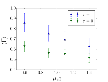
(a)

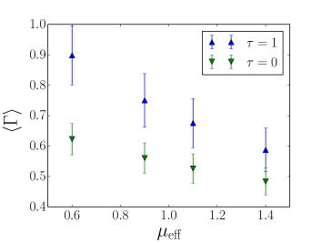
(b)

Figure 1: Average radial particle flux $\langle\Gamma\rangle$ for varying effective ion mass $\mu_{\mathrm{eff}}$, with and without FLR effects for warm and cold ions, respectively. Electrostatic $\widehat{\beta}=0$ (top) and electromagnetic $\widehat{\beta}=1$ (bottom).

We now test that the isotope mass effect found above is actually robust with variation of the collisionality parameter $C$ from $1$ to $7$. Results are shown in Figure 2. Plasma compositions considered are close to pure cases, i.e. H denotes a 99 % protium plasma with 1 % deuterium. D is pure deuterium and T denotes 99 % tritium with 1 % deuterium. It can be seen that transport levels for each species increase with larger collisionality $C$, which is consistent with standard benchmark cases [24]. The isotope effect is present throughout this range of collisionalities, which indicates that the collisional response, which mainly governs the parallel electron dynamics for the present range of parameters is not the only and major mechanism acting on transport reduction with respect to isotope mass.

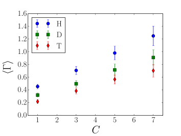
(a)

Figure 2: Average radial particle flux $\langle\Gamma\rangle$ as a function of electron-ion collisionality parameter $C$ for pure H, D and T plasmas.

4.2 Mass effects on zonal flows and GAMs

We next examine the role of zonal flows on the reduction of turbulent transport with increasing effective mass.

In Figure 3 (top) the ratio between zonal flow (ZF) energy $U=\sum_{s}a_{s}\int\mathrm{d}x\langle\phi_{s}\rangle\langle n_{s}\rangle/2$, where $\langle\cdot\rangle=\int\mathrm{d}y\mathrm{d}z$ is the flux-surface average, and total turbulent kinetic energy $E=\sum_{s}a_{s}\int\mathrm{d}x\rmd y\rmd z\phi_{s}n_{s}/2$ as a measure for the zonal flow strength is plotted as a function of the effective mass. While the ZF strength is generally larger for the warm ion case, both cold and warm ion cases show little dependence of the ZF strength on the effective mass: for $\tau_{i}=0$ the ZF energy ratio is nearly unaffected, and for $\tau_{i}=1$ it increases by approximately 5 $\%$ when varying from $\mu_{\mathrm{eff}}=0.6$ to $1.4$.

Another mechanism by which ZFs may reduce radial transport is by poloidal flow shear. Here, the shearing rate $\omega_{E}$ is defined as the inverse auto-correlation time of $\partial_{x}^{2}\langle\phi\rangle(x_{p})$, averaged over six distinct radial positions $x_{p}$. This is shown in Figure 3 (bottom), again for cold and warm ions. While the shearing rates on average are about 40 $\%$ stronger for the warm ion case compared to cold ion case, they are again nearly unchanged (within statistical uncertainties) for variations of the effective mass.

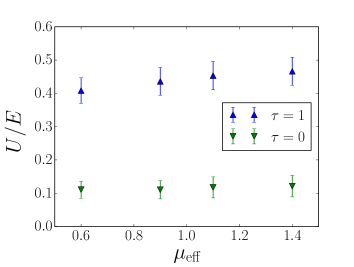
(a)

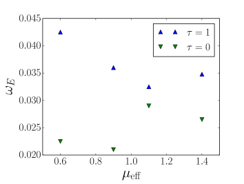
(b)

Figure 3: Top: Relative zonal flow energy intensity $U/E$ as a function of effective ion mass $\mu_{\mathrm{eff}}$ for warm and cold ions. Bottom: Zonal flow shearing rate $\omega_{E}$ for cold- and warm-ions.

We have conducted analyses of a number of further statistical quantities as a function of the effective mass.

Characteristic time scales $\tau_{c}$ can be deduced from auto-correlation functions, where state variables are sampled at each time step to produce time-series at $x_{p}$. Figure 4 shows, both for density (top) and potential (bottom) auto-correlation times, the general trend of longer time scales as the effective plasma mass increases. This trend is in approximate agreement with the shift of the drift wave frequency $\omega\sim 1/(1+\mu_{\mathrm{eff}})$ for the wave number scale $(\rho_{0}k_{\perp})=1$, and thus $\tau_{c}\sim 1+\mu_{\mathrm{eff}}$: the time scale increases by around 50 $\%$ when varying the effective mass from $\mu_{\mathrm{eff}}=0.6$ to $1.4$.

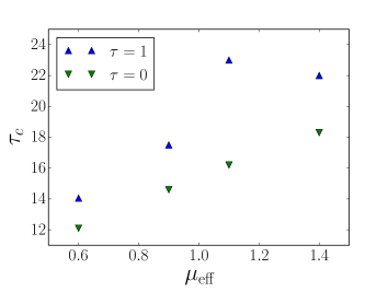
(a)

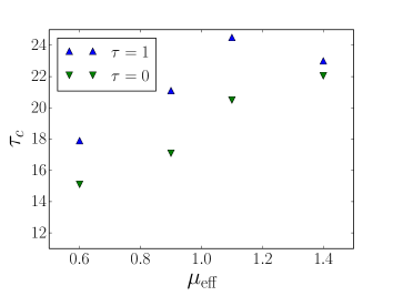
(b)

Figure 4: Correlation times for density (top) and potential (bottom).

As shown in Figure 5, we also find an increase in the maximum of the cross-correlation between density and potential fluctuations for warm ions, but not for the cold ion case. Values stem from averages of correlation times and cross-correlations over two time series at two distinct locations on the outboard midplane.

Typical values of the cross-correlation coefficient computed for the warm ion case are approximately a third weaker than in the cold ion case, but increase with effective mass as opposed to the cold ion case. From these trends we can infer that, first, the general reduction of cross-correlation for warm ions is a result of the $\tau_{i}$ dependence in the diamagnetic curvature coupling, which facilitates a trend towards a more interchange-like phase shift distribution and thus weaker cross-correlation. Second, the increase of the cross correlation with effective mass for the warm ions then can be attributed to warm ion dynamics, which by gyro-averaging counteract the phase shift.

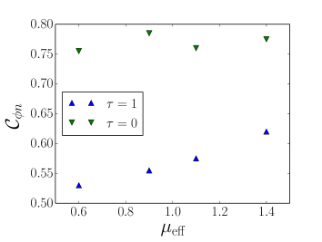
(a)

Figure 5: Maximum cross-correlation between density and potential for cold and warm ions.

Figure 6 shows correlation lengths $L_{y}$ in the perpendicular $y$-direction of the density, electric potential, and vorticity fields. For all cases we find that $L_{y}$ increases by approximately 20 $\%$ when varying the effective mass from $0.6$ to $1.4$. As the scaling is similar for both cold and warm ions, we infer that this trend could be based on the drift-scaling (which is independent of $\tau_{i}$ in contrast to direct FLR effects) by the effective mass acting on the polarisation.

On the other hand, an increase of perpendicular correlation lengths could also be attributed to stronger zonal flows. Here, the results allow no unambiguous conclusion: while the relative ZF strength and the shearing rate both only show weak dependence on the effective mass for warm ions and not at all for cold ions, the perpendicular (“poloidal”) correlation length increases for both cold and warm ions by around 20 $\%$.

In the context of the present (isothermal) gyro-fluid model, turbulence driven zonal flows thus only play a rather minor role as cause for the overall isotope effect on turbulent transport reduction.

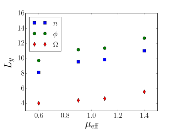
(a)

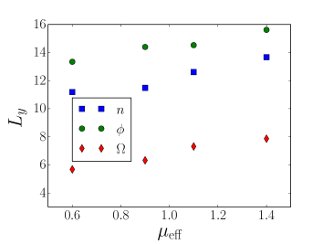
(b)

Figure 6: Correlation lengths for cold- (top) and warm ions (bottom).

Regarding the influence of isotope mass on GAMs, we have found no dependence of the GAM intensity (quantified by the spectral power of $\langle\phi\rangle$ at the GAM frequency) in our isothermal gyro-fluid simulations for the reference parameters.

We observe that in regions of strong flow shear, i.e. close to the radial boundaries, the ZFs are strong and the GAM activity is weak, whereas the ZF activity is weak in the center of the radial domain and GAMs are strong, consistent with energetic exchange of flux-surface averaged kinetic flow energy between zonal flows and GAMs.

4.3 Mass effects through finite Larmor radius and polarisation

In order to separate the mass effects acting through FLR terms or the drift scaling of polarisation, we set up a number of computations with artificially modified equations.

First, we study the effect of mass on transport through polarisation by modifying the standard cold ion case. Set one of simulations is run with the usual effective mass defined by $\mu_{\mathrm{eff}}=a_{i}\mu_{i}+a_{j}\mu_{j}$ given by separate mass ratios $\mu_{i}$ and $\mu_{j}$, here taken for hydrogen and deuterium masses, respectively. Set two is run with artificially setting $\mu_{i}=\mu_{j}$ in the effective mass entering in the polarisation. We perform both sets of runs with ion concentrations $a_{\mathrm{H}}:a_{\mathrm{D}}=80:20$ and $a_{\mathrm{H}}:a_{\mathrm{D}}=20:80$, denoted by ”light” and ”heavy”, respectively. The resulting transport rates are given in Figure 7 (data points are shifted slightly for better visibility). We find that the modified mass dependence in the vorticity term of the polarisation equation effectively annihilates the isotope effect, confirming the above assumptions. This now is not surprising any more, since for cold ions this term is the only mass-dependent term of relevance in the equations.

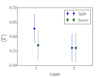
(a)

Figure 7: Average radial particle flux $\langle\Gamma\rangle$ for standard model ($\rmi$) and modified model ($\rmi\rmi$).

Performing similar modifications in order to focus on specific FLR effects only is a bit more tedious for the warm ion case, since both gyro-averaging operators are mass dependent. We recall the warm ion gyro-screening term, $(\Gamma_{0,s}-1)/\tau_{s}=-\mu_{s}k_{\perp}^{2}/(1+\mu_{s}\tau_{s}k_{\perp}^{2})$, occuring in the polarisation equation with the vorticity; and the gyro-averaging operator, $\Gamma_{1,s}=1/(1+\mu_{s}\tau_{s}k_{\perp}^{2})$, present in the averaging of density as part of the polarisation equation and acting on the potential in curvature and parallel terms. The latter is most significantly as part of the $\mathbf{E}\times\mathbf{B}$ advection.

We introduce three modifications of the model to artificially enhance and study the relative importance of each of these FLR effects.

• Case 1 denotes the original model.

• In case 2 we set $\Gamma_{0,i}=\Gamma_{0,j}$ in the “vorticity” term without modifying the FLR operators elsewhere.

• Case 3 leaves $\Gamma_{0,s}$ unaltered, but sets $\Gamma_{1,i}=\Gamma_{1,j}$ on the gyro-fluid densities in the polarisation equation (and also in the ”vorticity-free” boundary condition). Other occurences of $\Gamma_{1,s}$ are left unchanged.

• Finally, case 4 considers the impact of the gyro-averaged potential in the advective terms by setting $\Gamma_{1,i}=\Gamma_{1,j}$ there without modifying it in the polarisation equation and vorticity boundary conditions.

Results for the particle transport for all cases are given in Figure 8, with data points shifted slightly for improved visibility where necessary. The stronger the separation of the results between the “light” and “heavy” cases deviates from the standard case 1 in Figure 8, the more pronounced is the mass effect in the three different modified cases 2–4, which highlight the relative importance in the FLR terms.

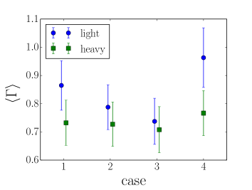
(a)

Figure 8: Average radial particle flux $\langle\Gamma\rangle$ for the warm ion standard model 1 and cases 2–4 as described in the text.

It can be seen that both mass-dependent FLR terms in the polarisation equation contribute significantly to the isotope effect. The main contribution is apparently caused by gyro-averaging on the gyro-fluid densities, whereas modification of gyro-screened advective terms actually leads to enhancement of the isotope effect.

4.4 Mass effects on ion inertia

We filter out inertia mass effects by introducing artifical electron-ion mass ratios for single-ion (D) computations, similar as in Bustos et al [13]. The electron mass is adjusted such that the ion-electron mass ratio is the same as for the regular cases discussed above. In this case the gyro-operators $\Gamma_{0}$ and $\Gamma_{1}$ are evaluated at $b=\rho_{0}^{2}k_{\perp}^{2}$, but the electron mass is varied according to $\mu_{\rme}\rightarrow\mu_{\rme}/\mu_{\mathrm{eff}}$, such that an isotope mass scaling is introduced in the inertia only. Results are shown in Figure 9.

For the cold ion case, there are no FLR effects and the only source for differences in transport levels is due to the plasma inertia.

We consider cases with $\mu_{\mathrm{eff}}=0.6$ and $\mu_{\mathrm{eff}}=1.4$ resulting from $\mathrm{H}:\mathrm{D}=80:20$ and $\mathrm{H}:\mathrm{D}=20:80$, respectively. In Figure 9 data points are shifted slightly around these values for better visibility.

For cold ions, both the adapted electron mass model and the reference model as expected yield comparable transport scaling, as expected.

For warm ions, we find that the relative inertia is only of rather minor importance compared to resolving the true gyro-radii. The isotope effect solely based on plasma inertia with identical Larmor radii is far weaker than the fully resolved case, indicating that the underlying mechanism is maintained from both inertia and FLR effects.

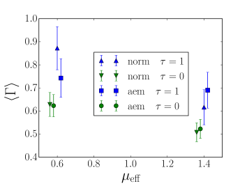
(a)

Figure 9: Average radial particle flux $\langle\Gamma\rangle$ for adapted electron masses (aem) compared to runs of the full model (norm).

4.5 Mass-adapted box and grid size test

Since a species Larmor radius $\rho_{s}^{2}=\mu_{s}\tau_{s}\rho_{0}^{2}\sim\mu_{\mathrm{eff}}$ we adapt the perpendicular simulation box size to yield the same number of gyro-radii per drift plane. This effectively increases the perpendicular resolution for $\mu_{\mathrm{eff}}<1$ and decreases it for $\mu_{\mathrm{eff}}>1$. Figure 10 shows results for $\mu_{\mathrm{eff}}=0.6$ and $\mu_{\mathrm{eff}}=1.4$ (data points are shifted where necessary for better visibility). These runs feature drift plane dimensions of $\{38\times 154\}\rho_{0}$ and $\{90\times 358\}\rho_{0}$ respectively. For all runs the number of nodes is $n_{x}\times n_{y}=64\times 256$.

Resulting transport levels in Figure 10 can be compared with the reference results labelled ’norm $\tau=0$’ and ’norm $\tau=1$’ in Figure 9, which are obtained from the standard resolution $\{96\times 256\}\rho_{0}\times 2\pi$ on $64\times 256\times 16$ nodes.

The mass-adapted resolution yields slightly higher transport levels for the light plasma and slightly lower transport levels for the heavy plasma (compared to the standard resolution). However, the isotope effect is still clearly visible. Hence the results shown in the previous subsections are not artificially modified by box size effects.

(a)

Figure 10: Average radial particle flux $\langle\Gamma\rangle$ for adapted simulation domain according to effective plasma mass.

The box size variations have taken into account possible effects of the vortex and zonal flow scales which fit into the computational domain.

Further computational or numerical artefacts could occur through the radial (Dirichlet) boundary conditions and through insufficient spatial resolution. We have also analysed the dependence of such computational errors on the isotope mass by means of the energy theorem. These results have confirmed that the employed resolution and treatment of boundary conditions do not significantly modify the overall isotope effects found in this work.

5 Discussion and conclusions

We have discussed ion isotope mass effects on electromagnetic gyro-fluid tokamak edge turbulence and zonal flows. The simulations show reduced transport amplitudes in heavier plasmas in terms of the reduced radial particle flux.

Zonal flow activity is found to be slightly enhanced with the isotope mass, but not to an extent to be able to (fully) explain the observed transport reduction. In the present model (isothermal, without mass dependent ion-ion collisions) we do not find any significant influence of isotope mass on GAM amplitudes.

The isotope effect is stronger for warm ions ($\tau_{i}=1$) but persists also for cold ion cases ($\tau_{i}=0$), which suggests that not FLR effects are the main mechanism for transport reduction, but ion inertia effects in the polarisation mediated by the mass-dependent drift scale. This is also supported by artificially adapting the electron mass relative to the ion mass to enhance pure ion inertia effects.

In the presented simulations with finite collisionality, electromagnetic flutter effects show no significant dependence on isotopes. However we note that in our present gyro-fluid model implementation the parallel magnetic vector potential is not subject to gyro-averaging operators, and thus electromagnetic FLR effects are neglected [16].

While the isotope effect is thus clearly present in the local isothermal gyro-fluid model, we still find a weaker influence on transport reduction and zonal flow enhancement compared to experimental results. This discrepancy could be caused by the neglect of thermal fluctuations and ion temperature gradient (ITG) and trapped electron mode (TEM) turbulence in the present model. Isotope mass effects on zonal flow damping via ion-ion collisionality and on neoclassical flows can be studied with full thermal models. In the future our delta-f gyro-fluid model is going to be extended to 6 moments including temperature fluctuations and a full-f approach, including consistent coupling of edge turbulence with scrape-off layer (SOL) fluctuations and filamentary transport.

References

References

- [1] Bessenrodt-Weberpals M et al1993 \NF33 1205
- [2] Hawryluk R J 1998 Rev. Mod. Phys.70 537
- [3] Tokar M Z, Kalupin D and Unterberg B 2004 Phys. Rev. Lett.92 215001
- [4] Waltz R 2004 Phys. Rev. Lett.93 239501
- [5] Tokar M Z 2004 Phys. Rev. Lett.93 239502
- [6] Scott B D 1997 Plasma Phys. Control. Fusion39 1635
- [7] Scott B D 1992 Plasma Phys. Control. Fusion35 1977
- [8] Dong J Q, Horton W and Dorland W 1997 Phys. Plasmas 1 3635
- [9] Lee W W and Santoro R A 1997 Phys. Plasmas 4 169
- [10] Xu Y et al2013 Phys. Rev. Lett.110 265005
- [11] Hahm T S, Wang L, Wang W X, Yoon E S and Duthoit F X 2013 \NF53 072002
- [12] Pusztai I, Candy J and Gohill P 2011 Phys. Plasmas 18 122501
- [13] A. Bustos A, Banon Navarro A, Görler T, Jenko F and Hidalgo C 2015 Phys. Plasmas 22 012305
- [14] Gurchenko A D et al2016 Plasma Phys. Control. Fusion58 044002
- [15] Scott B D 2003 Plasma Phys. Control. Fusion45 A385
- [16] Scott B D 2005 Phys. Plasmas 12 102307
- [17] Scott B D 1998 Phys. Plasmas 5 2334
- [18] Scott B D 2001 Phys. Plasmas 8 447
- [19] Scott B D 2007 Plasma Phys. Control. Fusion49 S25
- [20] Arakawa A 1966 J. Comput. Phys. 1 119
- [21] G.E. Karniadakis G E, Israeli M and Orszag S A 1991 J. Comput. Phys. 97 414
- [22] Naulin V and Nielsen A 2003 J. Sci. Comput. 25 104
- [23] Kendl A 2014 Int. J. Mass Spectrometry 365/366 106–113
- [24] Falchetto G L et al2008 Plasma Phys. Control. Fusion50 124015
- [25] Madsen J et al2011 Phys. Plasmas 18 112504
- [26] Dorland W et al1993 \PFB 5.3 812–835
- [27] Kendl A and Scott B D 2006 Phys. Plasmas 13 012504
- [28] Kendl A, Scott B D, Ball R and Dewar R L 2003 Phys. Plasmas 10 3684
- [29] Hasegawa A and Wakatani M 1983 Phys. Rev. Lett.50 682