Self-consistent continuum random-phase approximation with finite-range interactions for charge-exchange excitations

Abstract

The formalism of the continuum random-phase approximation theory which treats, without approximations, the continuum part of the single-particle spectrum, is extended to describe charge-exchange excitations. Our approach is self-consistent, meaning that we use a unique, finite-range, interaction in the Hartree-Fock calculations which generate the single-particle basis and in the continuum random-phase approximation which describes the excitation. We study excitations induced by the Fermi, Gamow-Teller and spin-dipole operators in doubly magic nuclei by using four Gogny-like finite-range interactions, two of them containing tensor forces. We focus our attention on the importance of the correct treatment of the continuum configuration space and on the effects of the tensor terms of the force.

I Introduction

The understanding of astrophysical nucleosynthesis, especially that induced by r processes, requires knowledge of charge-exchange excitations in unstable nuclei which, at least at the moment, have not been experimentally investigated arn07 . For this reason, there is a remarkable effort to construct nuclear structure models that can be applied in all the regions of nuclear chart, even to those nuclei where the experimental information is absent.

The random-phase approximation (RPA) theory boh52 , is one of the approaches more often used to describe nuclear collective excitations, and the original formulation for its application to nuclear systems row70 has been extended to study charge-exchange excitations hal67 ; lan80 ; aue81 ; aue83 . The largest part of the first applications of the RPA used phenomenological inputs. In the spirit of the Landau-Migdal theory of finite Fermi systems mig67 , the parameters of the mean-field potential, generating single-particle (s.p.) wave functions and energies, and those characterizing the interaction were suitably chosen to reproduce some experimentally known properties of the nucleus under study. Despite its success ost92 ; har01 ; ich06 , the application of this phenomenological approach is limited to those nuclei whose ground state properties are experimentally known.

The so-called self-consistent approaches overtake these limitations. The s.p. wave functions and energies are produced by Hartree-Fock (HF) calculations which use the same effective interaction employed in the RPA. The only input here is the effective interaction, and the values of the parameters characterizing the force are chosen once forever in a global fit of ground state properties involving a large set of nuclei distributed in the various regions of the nuclear chart cha07t . Once the force parameters have been selected by the fit procedure, the self-consistent calculations are parameter free and they can be applied to evaluate, and predict, the properties of every nucleus, independently of the experimental information about it.

Self-consistent studies of charge-exchange excitations have been conducted mainly with zero-range interactions of Skyrme type ham00 ; fra07 . Recently, these interactions have been implemented with tensor terms, and the effects of these new terms on charge-exchange excitations have been studied bai09a ; bai09b ; bai10 ; bai11a ; bai11b ; min13 . Zero-range effective interactions have the great merit of simplifying the calculations. There are, however, various drawbacks in their use, many of them discussed already in Ref. dec80 where the D1 parametrization of the finite-range Gogny interaction was proposed.

From the physics point of view, the present article is the natural continuation of the work of Ref. don14b where we presented results of charge-exchange responses calculated within the HF plus RPA (HF+RPA) framework with finite-range interactions. In that work, the s.p. configuration space was artificially discretized by setting boundary conditions at the edge of the radial integration box in the HF calculation. The RPA calculations were carried out by using this discrete s.p. configuration space whose dimensions are large enough such as the results obtained are independent on the eventual enlargement of this space. We call this type of calculations discrete RPA (DRPA) .

In Ref. don14b we applied our DRPA model to study charge-exchange excitations in ⁴⁸Ca, ⁹⁰Zr, and ²⁰⁸Pb nuclei, and we obtained satisfactory results in the description of the experimental centroid energies of these excitations. Since part of the charge-exchange strength lies above the particle emission threshold, we wonder whether the use of a discrete configuration space could affect our results. This worry is more relevant for neutron-rich nuclei where the particle emission threshold is lower than in the doubly closed shell nuclei we had investigated.

From the theoretical point of view the present work is the natural extension of Ref. don11a , where we introduced an RPA formalism that fully considers the continuum s.p. configuration space in the description of charge-conserving excitations. In the present article, for the reasons discussed above, we extend this continuum RPA (CRPA) method to the description of charge–exchange excitation modes. To the best of our knowledge, these are the first self-consistent CRPA calculations for charge-exchange excitations carried out with finite-range interactions.

In Sec. II we present the set of equations which defines our HF+CRPA model for charge-exchange excitations. The technical details of the calculations and the effective interactions used in our investigation are described in Sec. III. In Sec. IV we show, and discuss, the results we have obtained by applying our model to a set of medium-heavy nuclei, and we address particular attention to the role played by the tensor force. Finally, in Sec. V we summarize the main results of our investigation and we draw our conclusions.

II The model

The CRPA formalism presented in Refs. don08t ; don09 ; don11a ; don11b ; co13 is constructed to handle the continuum s.p. configuration space without approximation, even when finite-range interactions are used. Its extension to charge-exchange excitations does not require new hypotheses, or approximations; however, it is not straightforward and it deserves to be presented with some detail.

The basic idea of our formalism is to rewrite the usual RPA secular equations rin80 , where the unknown variables are the $X$ and $Y$ amplitudes, in terms of new unknowns called channel functions defined as

$$f^{{p_{0}h_{0}}}_{ph}(r)\,=\,\sum\!\!\!\!\!\!\!\!\int_{\epsilon_{p}}\,X^{{p_{0}h_{0}}}_{ph}(\epsilon_{p})\,R_{p}(r,\epsilon_{p})\,=\,R_{p_{0}}(r,\epsilon_{p_{0}})\,\delta_{pp_{0}}\,\delta_{hh_{0}}\,+\,\sum_{\mu}\,c^{\mu+}_{ph}\,\widetilde{\Phi}^{\mu+}_{p}(r)$$ (1)

and

$$g^{{p_{0}h_{0}}}_{ph}(r)\,=\,\sum\!\!\!\!\!\!\!\!\int_{\epsilon_{p}}\,\left[Y^{{{p_{0}h_{0}}}}_{ph}(\epsilon_{p})\right]^{*}\,R_{p}(r,\epsilon_{p})\,=\,\sum_{\mu}\,c^{\mu-}_{ph}\,\widetilde{\Phi}^{\mu-}_{p}(r)\,.$$ (2)

The definition of the $f$ and $g$ functions is given by the first equalities where the symbol $\sum\!\!\!\!\!\!\displaystyle\int$ indicates the sum on discrete s.p. energies and the integration on the continuum part of the spectrum, and $R_{p}$ is the radial part of the particle wave function. The label $p_{0}h_{0}$ indicates the elastic channel, defined as the specific channel where the particle is emitted. The number of elastic channels does not, usually, coincide with that of the particle-hole ($ph$) pairs, since the particle channel must be open; in other words, in an elastic channel the energy of the particle state must be positive, i.e. in the continuum. This implies that the excitation energy $\omega$ of the full system must be larger, in absolute value, than the energy of the hole state $\epsilon_{h}$. The CRPA equations are solved by imposing, every time, that the particle is emitted in a different elastic channel.

The second equalities of Eqs. (1) and (2) indicate that, in our approach, we expand the channel function on a basis. Specifically, we use a set of orthonormal Sturm functions raw82

$$\widetilde{\Phi}^{\mu}_{p}(r)\,=\,\Phi^{\mu}_{p}(r)\,-\,\sum_{\epsilon_{i}<\epsilon_{\rm F}}\,\delta_{l_{i},l_{p}}\,\delta_{j_{i},j_{p}}\,R^{*}_{i}(r)\,\int{\rm d}r^{\prime}\,r^{\prime 2}\,R_{i}(r^{\prime})\,\Phi^{\mu}_{p}(r^{\prime})\,$$ (3)

In Eqs. (1) and (2) the superscripts $+$ and $-$ indicate that the Sturm functions are calculated for $\epsilon_{p}=\epsilon_{h}+\omega$ or $\epsilon_{p}=\epsilon_{h}-\omega$, respectively, and we have dropped the explicit dependence on the open channel label $p_{0}h_{0}$ of all the $c^{\mu}_{ph}$ expansion coefficients to simplify the writing.

The charge-exchange excitations can be classified as isospin lowering $T_{-}$, when the hole is a neutron and the particle is a proton, and isospin rising $T_{+}$, in the opposite case. We use the convention of indicating with $\pi$ and $\nu$ a proton and a neutron state, respectively, and with a bar a hole state. Therefore, we have $\pi\overline{\nu}$ pairs in $T_{-}$  , and $\nu\overline{\pi}$ pairs in $T_{+}$  excitations.

We show in the Appendix A that charge-exchange CRPA ($pn$-CRPA) secular equations for $T_{-}$  excitations can be expressed as

$$\begin{bmatrix}A^{\mu+}_{\pi\overline{\nu},\pi^{\prime}\overline{\nu}^{\prime}}&-B^{\mu+}_{\pi\overline{\nu},\nu^{\prime}\overline{\pi}^{\prime}}\\ -(B^{\mu-}_{\nu\overline{\pi},\pi^{\prime}\overline{\nu}^{\prime}})^{*}&(A^{\mu-}_{\nu\overline{\pi},\nu^{\prime}\overline{\pi}^{\prime}})^{*}\\ \end{bmatrix}\begin{bmatrix}c^{\mu+}_{\pi^{\prime}\overline{\nu}^{\prime}}\\ (c^{\mu-}_{\nu^{\prime}\overline{\pi}^{\prime}})^{*}\\ \end{bmatrix}=\begin{bmatrix}C_{\pi\overline{\nu},\pi_{0}\overline{\nu}_{0}}\\ (D_{\nu\overline{\pi},\pi_{0}\overline{\nu}_{0}})^{*}\\ \end{bmatrix}\,,$$ (4)

and for $T_{+}$  excitations as

$$\begin{bmatrix}A^{\mu+}_{\nu\overline{\pi},\nu^{\prime}\overline{\pi}^{\prime}}&-B^{\mu+}_{\nu\overline{\pi},\pi^{\prime}\overline{\nu}^{\prime}}\\ -(B^{\mu-}_{\pi\overline{\nu},\nu^{\prime}\overline{\pi}^{\prime}})^{*}&(A^{\mu-}_{\pi\overline{\nu},\pi^{\prime}\overline{\nu}^{\prime}})^{*}\\ \end{bmatrix}\begin{bmatrix}c^{\mu+}_{\nu^{\prime}\overline{\pi}^{\prime}}\\ (c^{\mu-}_{\pi^{\prime}\overline{\nu}^{\prime}})^{*}\\ \end{bmatrix}=\begin{bmatrix}C_{\nu\overline{\pi},\nu_{0}\overline{\pi}_{0}}\\ (D_{\pi\overline{\nu},\nu_{0}\overline{\pi}_{0}})^{*}\\ \end{bmatrix}\,.$$ (5)

The explicit expressions of the $A$ and $B$ interaction matrix elements of the above equations are given in Appendix A, where it is shown that they depend on the excitation energy. Since Eqs. (4) and (5) are, separately, inhomogeneous sets of linear algebraic equations, they have solutions, different from the trivial one, for each value of $\omega$ above the nucleon emission threshold. As already stated, these equations are solved for each elastic channel, whose number is always equal to that of the open channels. The knowledge of the expansion coefficients $c^{\mu\pm}$ allows us to reconstruct the channel functions, as indicated by Eqs. (1) and (2). In particular, for a $T_{-}$  excitation we have $c^{\mu+}_{\nu^{\prime}\overline{\pi}^{\prime}}=c^{\mu-}_{\pi^{\prime}\overline{\nu}^{\prime}}=0$, therefore only $f_{\pi^{\prime}\overline{\nu}^{\prime}}^{\pi_{0}\overline{\nu}_{0}}$ and $g_{\nu^{\prime}\overline{\pi}^{\prime}}^{\pi_{0}\overline{\nu}_{0}}$ are different from zero. In contrast, if the reaction is of $T_{+}$  type, we have $c^{\mu+}_{\pi^{\prime}\overline{\nu}^{\prime}}=c^{\mu-}_{\nu^{\prime}\overline{\pi}^{\prime}}=0$, consequently only $f_{\nu^{\prime}\overline{\pi}^{\prime}}^{\nu_{0}\overline{\pi}_{0}}$ and $g_{\pi^{\prime}\overline{\nu}^{\prime}}^{\nu_{0}\overline{\pi}_{0}}$ are different from zero.

For a given excitation energy, and for each elastic channel, the full set of CRPA function channels $f$ and $g$ allows us to calculate the nuclear response induced by an external operator ${\cal Q}^{{\cal N}\pm}_{J^{\Pi},M}$. In our calculations, we consider one-body operators of the form

$${\cal Q}^{{\cal N}\,\pm}_{J^{\Pi},M}({\bf r})\,=\,\sum_{i=1}^{A}\,\kappa^{\cal N}_{J}(r_{i})\,\theta^{\cal N}_{J^{\Pi},M}(\Omega_{i})\,\delta({\bf r}_{i}-{\bf r})\,t_{\pm}(i)\,,$$ (6)

where the dependence on the radial, angular-spin, and isospin quantum numbers is factorized. For the transition matrix element we obtain the expression

$$\Gamma_{J^{\Pi}}^{{\cal N}\,\pm}(\omega) = \,\sum_{p_{0}h_{0}}\Big{|}\sum_{ph}\,\left[\langle j_{p}\|\theta^{\cal N}_{J^{\Pi}}\|j_{h}\rangle\,\langle\frac{1}{2}t_{p}|t_{\pm}|\frac{1}{2}t_{h}\rangle\,\int{\rm d}r\,r^{2}\,(f^{{p_{0}h_{0}}}_{ph}(r))^{*}\,\kappa^{\cal N}_{J}(r)\,R_{h}(r)\right.$$

$$\left.+\,(-1)^{J+j_{p}-j_{h}}\,\langle j_{h}\|\theta^{\cal N}_{J^{\Pi}}\|j_{p}\rangle\,\langle\frac{1}{2}t_{h}|t_{\pm}|\frac{1}{2}t_{p}\rangle\,\int{\rm d}r\,r^{2}\,R^{*}_{h}(r)\,\kappa^{\cal N}_{J}(r)\,g^{{p_{0}h_{0}}}_{ph}(r)\right]\Big{|}^{2}\,,$$

where with the double bar we indicate the reduced matrix elements, as defined in edm57 . In the previous equations we used $t_{\pm}=\tau_{\pm}/2$, where $\tau_{+}$ and $\tau_{-}$ are the isospin operators transforming, in our convention, a proton into a neutron and vice versa.

In the present work we consider the Fermi (${\cal N}\equiv{\rm F}$),

$${\cal Q}_{0^{+},0}^{{\rm F}\pm}\,=\,\sum_{i=1}^{A}\,t_{\pm}(i)\,,$$ (8)

and the Gamow-Teller (${\cal N}\equiv{\rm GT}$),

$${\cal Q}_{1^{+},M}^{{\rm GT}\pm}\,=\,\sum_{i=1}^{A}\,\mbox{\boldmath$\sigma$}_{M}(i)\,t_{\pm}(i)\,=\,\sqrt{4\pi}\,\sum_{i=1}^{A}\,[Y_{0}(i)\otimes\mbox{\boldmath$\sigma$}(i)]^{1}_{M}\,t_{\pm}(i)\,,$$ (9)

operators that excite $0^{+}$ and $1^{+}$ states, respectively. In the above equation we have indicated with $Y_{L}$ the spherical harmonics and with $\sigma$ the Pauli matrix operator acting on the spin variable. The symbol $\otimes$ indicates the usual tensor product between irreducible spherical tensors edm57 .

Finally, we have also studied the excitations induced by the spin dipole (${\cal N}\equiv{\rm SD}$) operator

$${\cal Q}_{J^{-},M}^{{\rm SD}\pm}\,=\,\sum_{i=1}^{A}\,r_{i}\,[Y_{1}(i)\otimes\mbox{\boldmath$\sigma$}(i)]^{J}_{M}\,t_{\pm}(i)\,,$$ (10)

which excites the multipoles $0^{-}$, $1^{-}$ and $2^{-}$. In this case, we calculate the strength functions corresponding to each individual multipolarity and also the total SD strength

$$\Gamma^{{\rm SD}\pm}(\omega)\,=\,\sum_{J^{\Pi}=0^{-},1^{-},2^{-}}\Gamma_{J^{\Pi}}^{{\rm SD}\pm}(\omega)\,\,.$$ (11)

In our study we have verified the sum-rule exhaustion, an important tool to investigate the global properties of the charge-exchange excitations. For this purpose, we have defined the sum-rule exhaustion function

$${\rm SR}_{J^{\Pi}}^{{\cal N}\,\pm}(\omega)\,=\,\int_{0}^{\omega}{\rm d}\omega^{\prime}\,\Gamma_{J^{\Pi}}^{{\cal N}\,\pm}(\omega^{\prime})\,.$$ (12)

We also found convenient to formulate the sum rules in terms of energy moments defined as

$$m_{\lambda}^{{\cal N}\,\pm}\,=\,\sum_{J^{\Pi}}\,m_{\lambda}(\Gamma^{{\cal N}\,\pm}_{J^{\Pi}})\,,$$ (13)

with

$$m_{\lambda}(\Gamma^{{\cal N}\,\pm}_{J^{\Pi}})\,=\,\int_{0}^{\infty}{\rm d}\omega\,\omega^{\lambda}\,\Gamma_{J^{\Pi}}^{{\cal N}\,\pm}(\omega)\,.$$ (14)

According to these expressions, we define the centroid energy of an excitation induced by the ${\cal N}$-type operator as

$${\omega}_{\rm cen}^{{\cal N}\,\pm}\,=\,\frac{m_{1}^{{\cal N}\,\pm}}{m_{0}^{{\cal N}\,\pm}}\,,$$ (15)

and the corresponding variance as

$${\cal V}^{{\cal N}\,\pm}\,=\,\frac{m_{2}^{{\cal N}\,\pm}}{m_{0}^{{\cal N}\,\pm}}\,-\,\left(\frac{m_{1}^{{\cal N}\,\pm}}{m_{0}^{{\cal N}\,\pm}}\right)^{2}\,.$$ (16)

In the case of the SD transitions, we have calculated the centroid of the distributions of the individual multipolarities,

$${\omega}_{{\rm cen},J^{\Pi}}^{{\rm SD}\pm}\,=\,\frac{m_{1}(\Gamma^{{\rm SD}\pm}_{J^{\Pi}})}{m_{0}(\Gamma^{{\rm SD}\pm}_{J^{\Pi}})}\,,$$ (17)

and also their corresponding variances. We carried out the numerical evaluations of Eq. (14) in a restricted energy range of which we shall indicate the minimum $(E_{<})$, and the maximum $(E_{>})$ values.

III Details of the calculations

The only input required by our self-consistent approach is the effective nucleon-nucleon force. In our calculations we consider a two-body nucleon-nucleon (NN) interaction of the form

$$V({\bf r}_{i},{\bf r}_{j})\,=\,\sum_{\eta}v_{\eta}(|{\bf r}_{i}-{\bf r}_{j}|)\,O^{\eta}_{i,j}\,,$$ (18)

where $v_{\eta}$ are scalar functions of the distance between the two interacting nucleons, and $O^{\eta}$ indicates the type of operator dependence:

$$O^{\eta}_{i,j} : 1\,,\,\,\mbox{\boldmath$\tau$}(i)\cdot\mbox{\boldmath$\tau$}(j)\,,\,\,\mbox{\boldmath$\sigma$}(i)\cdot\mbox{\boldmath$\sigma$}(j)\,,\,\,\mbox{\boldmath$\sigma$}(i)\cdot\mbox{\boldmath$\sigma$}(j)\,\mbox{\boldmath$\tau$}(i)\cdot\mbox{\boldmath$\tau$}(j)\,,$$ (19)

$$S(i,j)\,,\,\,S(i,j)\mbox{\boldmath$\tau$}(i)\cdot\mbox{\boldmath$\tau$}(j)\,,\,\,{\bf l}_{ij}\cdot{\bf s}_{ij}\,,\,\,{\bf l}_{ij}\cdot{\bf s}_{ij}\,\mbox{\boldmath$\tau$}(i)\cdot\mbox{\boldmath$\tau$}(j)\,.$$

In the above expression we have indicated with $\tau$ the Pauli matrix operator acting on the isospin variable, with ${\bf s}_{ij}$ the total spin of the interacting nuclear pair, with ${\bf l}_{ij}$ its orbital angular momentum, and with

$$S(i,j)\,=\,3\,\frac{[\mbox{\boldmath$\sigma$}(i)\cdot({\bf r}_{i}-{\bf r}_{j})]\,[\mbox{\boldmath$\sigma$}(j)\cdot({\bf r}_{i}-{\bf r}_{j})]}{({\bf r}_{i}-{\bf r}_{j})^{2}}\,-\,\mbox{\boldmath$\sigma$}(i)\cdot\mbox{\boldmath$\sigma$}(j)$$ (20)

the usual tensor operator. The terms $\eta=7,8$ include the spin-orbit contributions of the force.

In this work we carried out calculations with four Gogny-like interactions: the D1M force gor09 , the more traditional D1S ber91 parametrization, and also with other two forces, D1MT2c and D1ST2c don14b , which we built by adding tensor terms to the two basic parametrizations.

For complete self-consistent calculations, also the Coulomb and spin-orbit terms of the interaction should be considered in both steps of our approach, i.e., the HF and the CRPA calculations. The Coulomb term is obviously not active in charge-exchange excitations. The spin-orbit term is neglected in our CRPA calculations. We have recently studied the relevance of these two terms of the interaction in charge-conserving HF+DRPA calculations and we found that their contribution is very small don14a .

The first step of our calculations consists of constructing the s.p. basis by solving the HF equations with the bound-state boundary conditions at the edge of the discretization box. The technical details concerning the iterative procedure used to solve the HF equations for a density-dependent finite-range interaction can be found in Refs. co98b ; bau99 . In our HF+CRPA formalism, we solve the HF equations only for those states under the Fermi surface.

The second step is the solution of the CRPA equations. The formalism developed in the previous section leads to a set of algebraic equations whose unknowns are the expansion coefficients $c^{\pm}_{ph}$. The number of coefficients, and therefore the dimensions of the complex matrix to diagonalize, is a numerical input of our approach. Since the expansion on a basis of Sturm functions is a technical artifact, the solution of the CRPA secular equations must be independent of the number of expansion coefficients. We tested the convergence of our results by controlling the values of the total photoabsorption cross section in ¹⁶O and ⁴⁰Ca nuclei. We reached stability up to the fifth significant figure with ten expansion coefficients, independently of the multipolarity and of the energy of the excitation don09 .

With this HF+CRPA model, we have carried out calculations for the ¹²C, ¹⁶O, ²²O, ²⁴O, ⁴⁰Ca, ⁴⁸Ca, ⁵⁶Ni, and ⁶⁸Ni. In these nuclei the hole s.p. levels are fully occupied and this fact eliminates deformations and minimizes pairing effects.

	proton					neutron
nucleus	s.p. level	D1M	D1Mt2c	exp		s.p. level	D1M	D1Mt2c	exp
12C	$1p_{3/2}$	13.82	13.56	15.96		$1p_{3/2}$	16.36	16.09	18.72
16O	$1p_{1/2}$	11.94	12.66	12.13		$1p_{1/2}$	15.14	15.88	15.66
22O	$1p_{1/2}$	23.67	25.49	23.26		$1d_{5/2}$	6.38	6.80	6.67
24O	$1p_{1/2}$	25.69	27.65	28.64		$2s_{1/2}$	4.11	4.07	4.19
40Ca	$1d_{3/2}$	8.86	9.58	8.32		$1d_{3/2}$	15.74	16.49	15.65
48Ca	$1d_{3/2}$	16.69	18.38	15.81		$1f_{7/2}$	9.33	9.72	9.94
56Ni	$1f_{7/2}$	6.86	6.54	7.16		$1f_{7/2}$	16.00	15.67	16.62

Table 1: Energy thresholds, in MeV, for proton and neutron emission of the nuclei considered in this work. The experimental values have been obtained as explained in the text by using the binding energies values taken from the compilations of Refs. bnlw ; aud03 .

IV Results

In this section we present some results obtained in our investigation of charge-exchange excitations induced by the F, GT, and SD operators in the aforementioned nuclei. We shall be concerned about the part of the strength lying above the emission particle threshold.

We give in Table 1 the energy thresholds for proton and neutron emission, for the various nuclei we have considered in the present work. In our model, these values are those of the s.p. energies of the last occupied level. By using the physical interpretation of s.p. energies given by Koopman’s theorem rin80 , we have calculated the experimental values as differences between the binding energies of the indicated nucleus and those of the nuclei with one fewer nucleon. The binding energies have been taken from the compilations of Refs. bnlw ; aud03 . This comparison with the experimental values gives an idea of the level of accuracy of our mean-field model in the description of measured quantities. The quality of our approach in the description of the ground state properties of the nuclei under investigation is discussed in detail in Ref. co12b .

Before discussing the RPA results, we point out some features of our approach related to the need of the proper treatment of the continuum part of the s.p. configuration space. All the calculations have been carried out by using the four interactions presented in Sec. III, but, to simplify the discussion, we present here only the results obtained with the D1M and D1MT2c forces, since the results obtained with the other two forces do not show relevant differences.

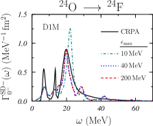
Figure 1: The contribution of the 0^- multipole to the $T_{-}$  SD response in ²⁴O, calculated in DRPA for different values of the s.p cut off energy $\epsilon_{\rm max}$ compared with the CRPA result shown by the full black line. The DRPA results are folded with a Lorentz function of 3 MeV width.

Figure 2: Energy distributions of the $T_{-}$  SD strengths for the ²⁴O nucleus obtained with the D1M interaction. In the upper panels we show, separately, the strengths of the $0^{-}$, $1^{-}$ and $2^{-}$ excitations, and in the two lowest panels, (g) and (h), their sums. The CRPA results are represented by the black solid curves. The vertical dotted blue lines show the DRPA results that generate the dashed red lines after a folding with a Lorentz function. The results obtained by using, in the folding procedure, a 3 MeV width are shown in the left panels, i.e. the (a), (c), (e) and (g) panels, and the results obtained with 1.2 MeV width are shown in the right panels.

blablablabla

We show in Fig. 1 the strength function for the $T_{-}$  excitation of the $0^{-}$ state induced by the SD operator in ²⁴O. This is a typical situation we have encountered. The full line represents the CRPA results obtained with the D1M interaction, and all the other lines the DRPA results folded with a Lorentz function of 3 MeV width. The various lines show the sensitivity of the DRPA results to the choice of the maximum energy of the s.p. configuration space, $\epsilon_{\rm max}$. The figure clearly shows that the convergence of the DRPA results is reached already for $\epsilon_{\rm max}$ = 40 MeV. The folding of the DRPA results cannot reproduce the smooth behavior of the CRPA strength above 20 MeV.

The limitations of the folding procedure are clarified in Fig. 2 where we show the results related to all the multipole excitations induced by the SD operator in the ²⁴O nucleus. In this figure, we indicate the original DRPA results, at convergence, with dotted vertical lines, to be compared with the full black curves representing the CRPA results. For each multipolarity, the position of the DRPA main peaks coincides with the maxima of the CRPA results. The two descriptions are rather similar in the lower energy region, but above 20 MeV, the DRPA produces peaks, while the CRPA responses have a rather smooth behavior. These peaks are clearly a consequence of the use of discrete s.p. basis.

The dashed red lines of the figure have been obtained by folding the DRPA with Lorentz functions. In the left panels the results have been obtained by using a width of 3 MeV, chosen to reproduce at best the CRPA $0^{-}$ response, while in the right panels the width is of 1.2 MeV because this value is more adequate to reproduce the CRPA $2^{-}$ response. The first choice generates a too large smoothing for the $2^{-}$ state, which is the dominant contribution, therefore the total SD^- response is much more spread than that of the CRPA. The second choice produces a global strength more similar to that of the CRPA, but fails in describing the CRPA results of the $0^{-}$ and $1^{-}$ excitations.

After having clarified the relation between the DRPA and CRPA results, we shall discuss, in order, the GT, F and SD excitations of the nuclei under investigation. In an extreme independent particle model (IPM), $N=Z$ nuclei with all the spin-orbit partner levels occupied cannot produce GT excitations. In our approach, which considers 1p-1h excitations only, the GT excitations for these nuclei are not prohibited but strongly hindered. The GT strength measured in ¹⁶O mer94 is about one order of magnitude larger than our RPA strength. As pointed out in Ref. bro94 only calculations considering, at least, 4p-4h excitations can produce the correct amount of strength.

Figure 3: Spectrum of the ¹⁶F nucleus as obtained from charge-exchange experimental experiments faz82 ; mer94 ; mad97 ; fuj09 . The energies are relative to the ¹⁶O ground state.

In Fig. 3 we compare the results of our RPA calculations with the spectrum of ¹⁶F obtained in charge-exchange experiments on the ¹⁶O target faz82 ; mer94 ; mad97 ; fuj09 . The order of magnitude of the excitation energies is reproduced, but the detailed structure of this spectrum is not well described. This requires the inclusion of excitations beyond 1p-1h.

Our RPA calculations are more adequate for nuclei where the GT excitation is related mainly to a 1p-1h excitation. We show in Fig. 4 the energy distribution of the $T_{-}$  GT for ⁴⁸Ca. The experimental data are those of Ref. yak09 . The full blue and dashed vertical lines show the DRPA results for the D1M and D1MT2c forces, respectively.

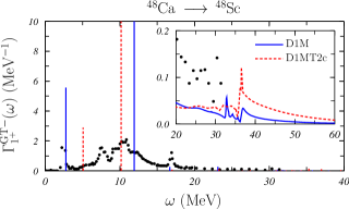
Figure 4: Energy distributions of the $T_{-}$  GT strength for the ⁴⁸Ca nucleus. The vertical lines show the results of the DRPA calculations carried out with the D1M (full blue lines) and D1MT2c (dashed red lines) interactions, respectively. In the inset we show the CRPA results. The full blue and dashed red curves indicate the CRPA results for the D1M and D1MT2c interactions, respectively. The experimental data are taken from Ref. yak09 .

The GT responses are dominated by the peaks shown in the main part of the figure. The strengths in the region above these main peaks are much smaller. We present in the inset of Fig. 4, the responses of the CRPA calculation in the region above 20 MeV, by using a different scale. The CRPA results obtained with D1M and D1MT2c interactions are indicated by the full blue and dashed red curves, respectively.

The DRPA calculations exhaust the so-called Ikeda sum rule at 1% level for the D1MT2c force and much better, to one part in over 100000, when the D1M interaction is used. For each of the two interactions, the DRPA calculations generate two peaks. The peak located at the lower energy, below the emission particle threshold, is dominated by the transition from the neutron $1f_{7/2}$ level to the bound proton $1f_{7/2}$ level. The second peak, whose excitation energy is above the emission particle threshold, is dominated by the transition from the neutron $1f_{7/2}$ level to the proton $1f_{5/2}$ level, which, in our calculations, is bound. Such RPA solutions with energy eigenvalues in the continuum but dominated by bound s.p. transitions are not well described by our CRPA formalism, tailored for the continuum. A meaningful comparison between DRPA and CRPA results should be done in the region beyond the two main peaks. In the region above 20 MeV, the DRPA and CRPA total strengths are very similar. The global DRPA strength of the $T_{-}$  GT transition for the D1M interaction is 24.17. The contribution of the region above the main peak is 1.05 to be compared with the CRPA integrated strength of 1.08. The agreement between DRPA and CRPA results for the D1MT2c interaction is not so precise. The total DRPA $T_{-}$  GT strength is 24.04 of which 1.18 is beyond the main peak. In this region, the CRPA total strength is 1.58.

The width of the experimental strength is much larger than that of the RPA calculations. We have already encountered this kind of problems in the comparison of our charge-conserving CRPA results with total photoabsorption cross sections don11a . It is a common feature of the RPA description of the giant resonances spe91 and it is attributed to its intrinsic limitation of considering one-particle one-hole excitations only. It is evident that the RPA strength needs a redistribution which will be provided by the inclusion of 2p-2h degrees of freedom gam12 . The results presented in the inset show a sudden increase of the CRPA responses above the 35 MeV due to the opening of the channels related to the emission of neutrons from the $1s_{1/2}$ s.p. level. This sharp peak of the CRPA response would be, probably, smoothed by the inclusion of 2p-2h excitations.

The total experimental strength is $15.36\pm 2.16$, corresponding to about 60% of the theoretical strength only. The measurements stop at an excitation energy of about 30 MeV, and our calculations indicate that there is GT strength above this energy. The presence of strength above the maximum energy measured in the experiment is probably the explanation of the missing GT strength. For example, analysis of the ⁹⁰Zr (p,n) ⁹⁰Nb data ich06 indicates that all the GT strength is present in the excitation, much of it above the main peak.

The difference between the positions of the main peaks of the DRPA results in ⁴⁸Ca, calculated with the D1M and D1MT2c forces is essentially due to the effect of the tensor force on the energy of the proton $1f_{5/2}$ level. Otsuka and collaborators ots05 pointed out that the tensor force when acting on s.p. levels with different isospin lowers the energy of the state with $j=l-1/2$ and increases that of the state with $j=l+1/2$. In this case the energy of the proton $1f_{5/2}$ level is lowered, and that of the $1f_{7/2}$ is enhanced by the tensor force. The RPA results shown in Fig. 4 are clearly affected by this effect. The energy of the first excited state, where the main p-h transition is on the proton $1f_{7/2}$ level, is increased, while that of the second state, that with the $1f_{5/2}$ level, is lowered. The effect of the tensor force on the RPA calculation in itself is negligible as compared with the effect on the s.p. energies.

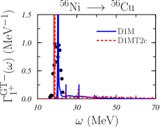
Figure 5: Energy distributions of the $T_{-}$  GT strength for the ⁵⁶Ni nucleus. The meaning of the lines is the same as that of Fig. 4. The data are taken from Ref. sas11 .

The points discussed for the GT excitation in ⁴⁸Ca can also be considered for the ⁵⁶Ni nucleus. We show in Fig. 5 the energy distribution of the $T_{-}$  GT strengths obtained with our DRPA and CRPA calculations and we compare them with the experimental data of Ref. sas11 . The meaning of the various lines is as in the previous figure.

In contrast to ⁴⁸Ca, the ⁵⁶Ni nucleus is a $N=Z$ nucleus, and, differently from ¹⁶O and ⁴⁰Ca , not all the spin-orbit partner levels are occupied. For this reason there are large GT excitation strengths from the $1f_{7/2}$ hole to the $1f_{5/2}$ particle state, in both the neutron-proton and proton-neutron cases. In effect the zero value predicted by the Ikeda sum rule for the $N=Z$ nuclei is obtained by subtracting the $T_{-}$  and $T_{+}$  total strengths which are about 12, much larger than the values $\sim 0.05$ and $\sim 0.1$ we found in ¹⁶O and ⁴⁰Ca , respectively.

Differently from the ⁴⁸Ca case, we observe in Fig. 5 that also the CRPA strength distributions present large peaks coinciding with the main peaks of the DRPA results. This is because the $1f_{5/2}$ s.p. states are unbound for both protons and neutrons, independently of the interaction, considered. Our CRPA formalism treats these states in the continuum, even though they appear as sharp resonances and produce rather narrow peaks in the energy distributions.

The comparison with the data indicates the need to consider in the calculations also the spreading width. The integrated experimental strength is about 3.6, i.e roughly the 30% of our RPA strength. On the other hand, the results of the figure show that there is considerable strength above the maximum measured energy. In our calculations this strength is about 10% of the total one in calculations both with and without tensor. Finally, we should recall that in our model ⁵⁶Ni is a doubly closed shell nucleus, but there are indications that pairing effects could be relevant bai13 .

In analogy with what we have already discussed for the GT transitions, also the F transitions are hindered in $N=Z$ nuclei. For nuclei with neutron excess the main peak is concentrated in the transition between the occupied neutron s.p. state and the empty isobaric analog proton state. Our DRPA calculations identify strong 0⁺ states at 3.35, 3.28, and 6.96 MeV in ²²O , ²⁴O and ⁴⁸Ca nuclei, respectively. All these states are below the continuum energy threshold. Unfortunately, in the low-energy spectra of the ²²F, ²⁴F and ⁴⁸Sc nuclei these states have not been identified. In the nuclei with neutron excess we have investigated, the $T_{-}$  F strength allocated in the continuum region is less than 1% of the total one. For the $N=Z$ nuclei studied, all the $T_{-}$  F strengths appear above the continuum threshold, and their total values are comparable to those found in the continuum part of strength of the nuclei with neutron excess.

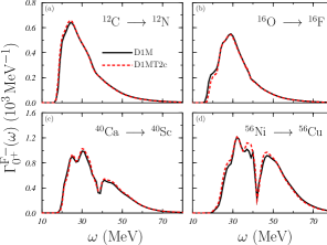
Figure 6: Energy distributions of the $T_{-}$  F responses obtained in CRPA calculations with the D1M (full black lines) and D1MT2c (dashed red lines) interactions.

As example of our results, we show in Fig. 6 the $T_{-}$  F responses for the ¹²C , ¹⁶O , ⁴⁰Ca and ⁵⁶Ni nuclei which have the same number of protons and neutrons. The responses of the ⁴⁰Ca and ⁵⁶Ni nuclei show two large peaks. These are due to the importance of different particle-hole transitions in the RPA response. In ⁵⁶Ni the lower energy peak is characterized by a p-h pair related to the $f_{7/2}$ s.p. states, while the peak at higher energy by a p-h pair related to the $d_{3/2}$ hole. In the case of the ⁴⁰Ca, both peaks are dominated by the $d_{5/2}$ p-h pair. The residual interaction in the RPA theory mixes this pair with the $d_{3/2}$ p-h pair in the lower energy peak and with the $p_{3/2}$ p-h pair in the higher energy peak. In the figure the full black lines show the F strengths obtained with the D1M interaction and the dashed red lines those found with D1MT2c. In this case, the tensor force does not produce remarkable effects.

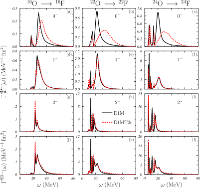
Figure 7: Energy distributions of the $T_{-}$  $\Gamma_{J^{\Pi}}^{{\rm SD}}(\omega)$ and $\Gamma^{{\rm SD}}(\omega)$ strengths for ¹⁶O , ²²O and ²⁴O nuclei obtained in CRPA calculations. The solid black curves have been obtained with the D1M interaction while the dashed red curves with the D1MT2c force.

We show in Figs. 7, 8, and 9 the $T_{-}$  SD strength distributions for all the nuclei we have considered. We present separately the contribution of each multipole, and also the total strength. As in the previous figures, the full black lines show the results obtained with the D1M interaction, while the dashed red lines show those obtained with D1MT2c. In these cases the size of the strength is comparable with that obtained in DRPA calculations don14b , since the main part of the strength is above the particle emission threshold. All the cases investigated indicate that the largest contribution to the total strength comes from the $2^{-}$ excitation, which is about one order of magnitude larger than that of the $0^{-}$, with the only exception being the ⁶⁸Ni nucleus, where it is three times larger.

The inclusion of the tensor force has a small influence on the $1^{-}$ and $2^{-}$ strength distributions, while the changes on the $0^{-}$ strength, the smallest one, are remarkable. In all the $0^{-}$ cases considered, the tensor force moves the peak of the resonance toward higher energies. In order to present a more quantitative information of this effect, we show in Table 2 the values of the centroid energies and of the variances of the $0^{-}$ main resonances shown in Figs. 7, 8 and 9. In general, the shift of the centroid energies is relevant and reaches a value of about $9\,$MeV, in the case of the ²²O, and ²⁴O nuclei. The effects on the variance, indicating a larger spreading of the $0^{-}$ width, are significant only in the oxygen isotopes.

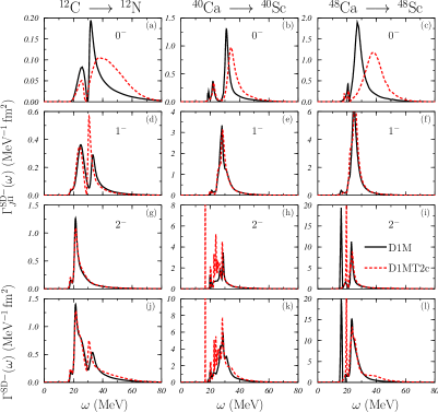
Figure 8: The same as in Fig. 7 for ¹²C , ⁴⁰Ca , and ⁴⁸Ca nuclei.

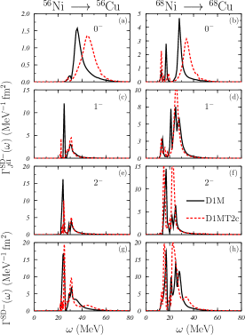
Figure 9: The same as in Fig. 7 for ⁵⁶Ni , and ⁶⁸Ni nuclei.

In our calculations with the D1MT2c interaction, the tensor is active in both HF and RPA calculations. In order to disentangle these two effects, in Fig. 10, we show the $0^{-}$ excitations for all the nuclei we have investigated. The dashed red curves have been obtained by using the D1MT2c interaction in both HF and CRPA calculations, and they coincide with those shown in Figs. 7, 8, and 9. The solid black curves indicate the results obtained in CRPA calculations by using the D1MT2c interaction but with the HF s.p. wave functions generated with the D1M force. The comparison between these results and the full lines of the $0^{-}$ excitations of Figs. 7, 8, and 9, indicates that the effect of the tensor is mainly present in the RPA, rather than in the modification of the s.p. wave functions.

			${\omega}_{{\rm cen},0^{-}}^{{\rm SD}-}$ (MeV)			${\cal V}_{0^{-}}^{{\rm SD}-}$ (MeV)
nucleus	$E_{<}$ (MeV)	$E_{>}$ (MeV)	D1M	D1MT2c		D1M	D1MT2c
16O	20.0	60.0	32.82	36.45		7.00	7.34
22O	16.7	60.0	26.35	35.28		7.57	8.67
24O	15.0	60.0	24.18	33.44		7.68	9.15
12C	29.6	60.0	38.67	43.62		7.38	7.64
40Ca	26.0	60.0	34.32	37.57		5.68	5.80
48Ca	21.4	60.0	30.63	39.12		6.42	6.79
56Ni	30.0	60.0	39.43	45.36		5.86	5.69
68Ni	20.0	50.0	30.33	35.24		4.62	4.60

Table 2: Values of the centroid energies and variances, as given by Eqs. (17) and (16), respectively, for the T_- SD, $J^{\Pi}=0^{-}$ multipole excitations, for the D1M and D1MT2c interactions. We have indicated with $E_{<}$ and $E_{>}$, in MeV, the extremes of the energy integral in Eq. (14).

A crucial test of the validity of the theoretical results is to check if the sum rules, obtained for the F, GT, and SD excitations by evaluating Eq. (12) for large values of the excitation energy, are satisfied according to the expected values. In Ref. don14b , we have shown that our DRPA self-consistent approach satisfies the sum rules within 0.1%. An analogous test with the CRPA calculations is more difficult, since a large part of the strength is distributed below the emission particle threshold, where this approach is not applicable. For this reason, we have added to the CRPA sum-rule exhaustion functions (12) the contribution of the DRPA below threshold and compared the result with the DRPA asymptotic values.

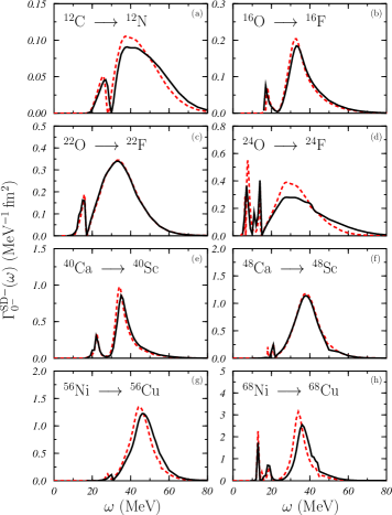
Figure 10: Energy distributions of the $T_{-}$  $\Gamma_{0^{-}}^{{\rm SD}}(\omega)$ obtained in CRPA calculations for the various nuclei studied. The dashed red curves correspond to the D1MT2c force. The solid black lines have been obtained by using the D1M s.p. wave functions together with the D1MT2c interaction in the CRPA calculations.

Figure 11: SD sum rule exhaustion, as given by Eq. (12), obtained in CRPA calculations for the ²²O nucleus. Left (right) panels correspond to the T_- (T₊) transitions. The full red curves show the results obtained with the D1M force and the dashed red curves those obtained with the D1MT2c force. The full and dashed horizontal black lines indicated the asymptotic values of the analogous DRPA results taken from Ref. don14b .

As example of this procedure, we show in Fig. 11 the results obtained with the three multipole excitations of the SD operator for the ²²O nucleus. The curves show the CRPA sum rule exhaustion functions (12) as a function of $\omega$, the upper limit of the integral. The full red curve was obtained with the D1M interaction while the dashed red curve was obtained with the D1MT2c interaction. The horizontal black lines indicate the asymptotic values we have obtained with the analogous DRPA calculations.

The agreement between the results of the two calculations is remarkable, even though we observe a slight overshooting in the $T_{+}$  responses for $1^{-}$ and $2^{-}$. For the $0^{-}$ multipolarity, the asymptotic value is reached more quickly in the D1M case than in the D1MT2c one. This is due to the shift of the peak of the resonance towards larger energy and to the bigger spreading of the strengths when tensor terms of the interactions are active, as we have already stressed and shown in Fig. 7 . It is remarkable the increase of the $T_{-}$  and $T_{+}$  strengths generated by the tensor term. We recall that the theoretical sum rule asymptotic value limiting the strength is obtained as a difference between the $T_{-}$  and $T_{+}$  strengths, which is conserved in all the $0^{-}$ calculations, with or without tensor force.

V Summary and conclusions

We have extended the CRPA formalism of Ref. don11a , which handles finite-range interactions and continuum s.p. configuration space without any approximation, to the description of charge-exchange excitations. In our calculations we used four Gogny-like finite-range interactions, two of them containing tensor terms, and we applied our formalism to describe the F, GT, and SD excitations in the ¹²C, ¹⁶O, ²²O, ²⁴O, ⁴⁰Ca, ⁴⁸Ca, ⁵⁶Ni, and ⁶⁸Ni nuclei. The goals of our work were:

1. the presentation of the non trivial extension of the charge-conserving CRPA formalism to treat charge-exchange excitations;

2. the comparison of CRPA results with those obtained in DRPA calculations;

3. the study of the effects of the tensor interaction in charge-exchange excitations, and

4. the comparison with the available experimental data.

Concerning the first goal, we have shown that it is possible to formulate the $pn$-CRPA secular equations in a form which allows us to obtain simultaneous solution of proton-neutron and neutron-proton excitations. This is analogous to the commonly used formulation of the $pn$-DRPA hal67 , as it has been used, for example, in Ref. don14b .

The comparison between CRPA and DRPA results has been carried out to test the stability of the DRPA calculations against the dimensions of the s.p. configuration space. We have obtained a very good agreement between the position of the DRPA peaks and that of the maxima of the CRPA strength. For a given multipole excitation, by using a folding procedure with a Lorentz function of appropriate width, we obtained agreement also with the CRPA strength distribution. Furthermore, we have also verified that the two types of calculations satisfy the sum rules with the same degree of accuracy.

We have pointed out the ambiguities of the folding procedure commonly used to generate continuous responses out of DRPA solutions. We have shown that the three CRPA components of the SD response cannot be simultaneously described by using a single Lorentz function. Having established the agreement between CRPA and DRPA results, we are confident on the use of DRPA calculations in situations where we cannot carry out CRPA calculations. These are, for example, the cases of excitations below the particle emission threshold, and the calculations for nuclei heavier than those treated in the present article.

Our formalism allows the use of effective nucleon-nucleon interactions of finite-range type which include tensor terms. In Ref. don14b we presented charge-exchange results obtained with the same interactions used here. The results shown in this reference have been obtained within the DRPA framework. The present work can be considered to complement that of Ref. don14b by considering the continuum.

The tensor force does not produce remarkable effects on the continuum part of the F and GT strengths, which, for nuclei with neutron excess, is only a small part of the total strength. The situation is different for the SD excitations whose strength develops mainly in the continuum. We have analyzed the $0^{-}$, $1^{-}$, and $2^{-}$ multipoles composing the SD responses for various nuclei and we found that the $2^{-}$ excitation is the most important of the three, dominating the total response. On the other hand, the $0^{-}$ strength is extremely sensitive to the tensor term. Its inclusion in the CRPA calculations moves the maxima of the $0^{-}$ responses towards higher energies. This shift is particularly remarkable in the oxygen isotopes where we found changes of the centroid energies of up to 9 MeV, and a significant widening of the width. We have verified that this large sensitivity of the $0^{-}$ to the tensor force is mainly related to the RPA calculations, and not to the modifications of the s.p. energies.

The fourth, and last, goal of our work was the comparison with the available data, which we have found mainly for the GT transitions. In our approach, which considers only 1p-1h excitations, the GT excitations are strongly hindered in nuclei with equal number of protons and neutrons and with spin-orbit partner levels fully occupied. The experimental strength of ¹⁶O mer94 is one order of magnitude larger than that of our CRPA calculations. Also the experimental spectrum of ¹⁶F obtained in charge-exchange experiments on the ¹⁶O target faz82 ; mer94 ; mad97 ; fuj09 is not described in detail by our approach, even though the order of magnitude of the excitation energies is reproduced. These are indications of the need to include higher order particle-hole excitations to improve the description of these data.

The comparison with the GT data in ⁴⁸Ca and ⁵⁶Ni shows the need to include the spreading width to obtain a detailed description of the experiment. On the other hand, the position of the main peaks of the resonance is rather well reproduced. The experimentally measured strengths in these two nuclei satisfy only part of the sum rule. Our calculations indicate that the GT strength above the measured highest excitation energy is not negligible. This finding is in agreement with the study of ⁹⁰Zr (p,n) ⁹⁰Nb data ich06 , where, by considering the strength lying beyond the main resonance, all the expected GT strength has been found.

Despite the limitations we have pointed out, our CRPA model, which considers all the continuum s.p. space without the need of artificial cuts, is a further step towards the construction of a parameter free mean-field approach describing nuclei in all the regions of the nuclear chart. We do not aim for a detailed description of low-lying spectra and strength distributions; however peak positions and global strengths can be well predicted by our approach, which can be applied also to unstable nuclei. This offers a great potential for the study of neutrino cross sections in the energy region around the emission particle threshold, in analogy to what has been done in Ref. bot05 for stable nuclei.

Appendix A $pn$-CRPA matrix elements.

In this Appendix we obtain the $pn$-CRPA equations. First we recall here the basic equations of our CRPA formalism. A more detailed description can be found in Refs. don08t ; don09 ; don11a .

For each excited state $|\alpha\rangle\equiv|J,\Pi,\omega\rangle$, characterized by its total angular momentum $J$, parity $\Pi$ and excitation energy $\omega$, we write a set of algebraic equations whose unknowns are the $c^{\mu}_{ph}$ expansion coefficients don08t ; don09

$$\sum_{\mu}\,\sum_{p^{\prime}h^{\prime}}\,\Bigg{\{}\Bigg{[}\delta_{pp^{\prime}}\,\delta_{hh^{\prime}}\Big{(}\delta_{\mu\alpha}\,-\,\langle(\Phi_{p}^{\alpha+})^{*}|{\cal U}|\Phi_{p}^{\mu+}\rangle\,+\,\langle(\Phi_{p}^{\alpha+})^{*}\,{\mathbb{I}}|{\cal W}|{\mathbb{I}}\,\Phi^{\mu+}_{p}\rangle$$ (21)

$$+\,\sum_{\epsilon_{i}<\epsilon_{\rm F}}\,\delta_{ip}\,(\epsilon_{i}-\epsilon_{h}-\omega)\,\langle(\Phi_{p}^{\alpha+})^{*}|R_{i}\rangle\langle(R_{i})^{*}|\Phi_{p}^{\mu+}\rangle\Big{)}$$

$$-\,\Big{(}\langle(\widetilde{\Phi}_{p}^{\alpha+})^{*}R_{h^{\prime}}|V^{J,{\rm dir}}_{ph,p^{\prime}h^{\prime}}|R_{h}\widetilde{\Phi}^{\mu+}_{p^{\prime}}\rangle\,-\,\langle(\widetilde{\Phi}_{p}^{\alpha+})^{*}R_{h^{\prime}}|V^{J,{\rm exc}}_{ph,p^{\prime}h^{\prime}}|\widetilde{\Phi}^{\mu+}_{p^{\prime}}R_{h}\rangle\Big{)}\Bigg{]}\,c^{\mu+}_{p^{\prime}h^{\prime}}\,$$

$$-\,\Big{(}\langle(\widetilde{\Phi}_{p}^{\alpha+})^{*}\widetilde{\Phi}^{\mu-}_{p^{\prime}}|U^{J,{\rm dir}}_{ph,p^{\prime}h^{\prime}}|R_{h}R_{h^{\prime}}\rangle\,-\,\langle(\widetilde{\Phi}_{p}^{\alpha+})^{*}\widetilde{\Phi}^{\mu-}_{p^{\prime}}|U^{J,{\rm exc}}_{ph,p^{\prime}h^{\prime}}|R_{h^{\prime}}R_{h}\rangle\Big{)}\,(c^{\mu-}_{p^{\prime}h^{\prime}})^{*}\Bigg{\}}\,=\,$$

$$=\,\langle(\widetilde{\Phi}_{p}^{\alpha+})^{*}R_{h_{0}}|V^{J,{\rm dir}}_{ph,p_{0}h_{0}}|R_{h}R_{p_{0}}(\epsilon_{p_{0}})\rangle\,-\,\langle(\widetilde{\Phi}_{p}^{\alpha+})^{*}R_{h_{0}}|V^{J,{\rm exc}}_{ph,p_{0}h_{0}}|R_{p_{0}}(\epsilon_{p_{0}})R_{h}\rangle$$

and

$$\sum_{\mu}\,\sum_{p^{\prime}h^{\prime}}\,\Bigg{\{}\Bigg{[}\delta_{pp^{\prime}}\,\delta_{hh^{\prime}}\Big{(}\delta_{\mu\alpha}\,-\,\langle(\Phi_{p}^{\alpha-})^{*}|{\cal U}|\Phi_{p}^{\mu-}\rangle\,+\,\langle(\Phi_{p}^{\alpha-})^{*}\,{\mathbb{I}}|{\cal W}|{\mathbb{I}}\,\Phi^{\mu-}_{p}\rangle$$ (22)

$$+\,\sum_{\epsilon_{i}<\epsilon_{\rm F}}\,\delta_{ip}\,(\epsilon_{i}-\epsilon_{h}+\omega)\,\langle(\Phi_{p}^{\alpha-})^{*}|R_{i}\rangle\langle(R_{i})^{*}|\Phi_{p}^{\mu-}\rangle\Big{)}$$

$$-\,\Big{(}\langle(\widetilde{\Phi}_{p}^{\alpha-})^{*}R_{h^{\prime}}|V^{J,{\rm dir}}_{ph,p^{\prime}h^{\prime}}|R_{h}\widetilde{\Phi}^{\mu-}_{p^{\prime}}\rangle\,-\,\langle(\widetilde{\Phi}_{p}^{\alpha-})^{*}R_{h^{\prime}}|V^{J,{\rm exc}}_{ph,p^{\prime}h^{\prime}}|\widetilde{\Phi}^{\mu-}_{p^{\prime}}R_{h}\rangle\Big{)}\Bigg{]}\,c^{\mu-}_{p^{\prime}h^{\prime}}\,$$

$$-\,\Big{(}\langle(\widetilde{\Phi}_{p}^{\alpha-})^{*}\widetilde{\Phi}^{\mu+}_{p^{\prime}}|U^{J,{\rm dir}}_{ph,p^{\prime}h^{\prime}}|R_{h}R_{h^{\prime}}\rangle\,-\,\langle(\widetilde{\Phi}_{p}^{\alpha-})^{*}\widetilde{\Phi}^{\mu+}_{p^{\prime}}|U^{J,{\rm exc}}_{ph,p^{\prime}h^{\prime}}|R_{h^{\prime}}R_{h}\rangle\Big{)}\,(c^{\mu+}_{p^{\prime}h^{\prime}})^{*}\Bigg{\}}\,=\,$$

$$=\,\langle(\widetilde{\Phi}_{p}^{\alpha-})^{*}R_{p_{0}}(\epsilon_{p_{0}})|U^{J,{\rm dir}}_{ph,p_{0}h_{0}}|R_{h}R_{h_{0}}\rangle\,-\,\langle(\widetilde{\Phi}_{p}^{\alpha-})^{*}R_{p_{0}}(\epsilon_{p_{0}})|U^{J,{\rm exc}}_{ph,p_{0}h_{0}}|R_{h_{0}}R_{h}\rangle\,.$$

In the above equations we have indicated, respectively, as ${\cal U}$ and ${\cal W}$ the Hartree and Fock-Dirac potentials as they are commonly defined in the HF formalism rin80 . The symbols $U$ and $V$ indicate the matrix elements of the nucleon-nucleon interaction, $R_{h}$ the s.p. radial wave function of a hole state of $\epsilon_{h}$ energy, and $R_{p}(\epsilon_{p})$ the s.p. radial wave function of a continuum particle state.

We simplify the writing of Eqs. (21) and (22) by defining the following quantities:

$$A^{\mu\pm}_{ph,p^{\prime}h^{\prime}} = \delta_{pp^{\prime}}\,\delta_{hh^{\prime}}\Big{(}\delta_{\mu\alpha}\,-\,\langle(\Phi_{p}^{\alpha\pm})^{*}|{\cal U}|\Phi_{p}^{\mu\pm}\rangle\,+\,\langle(\Phi_{p}^{\alpha\pm})^{*}\,{\mathbb{I}}|{\cal W}|{\mathbb{I}}\,\Phi^{\mu\pm}_{p}\rangle$$ (23)

$$\hskip 65.44142pt+\,\sum_{\epsilon_{i}<\epsilon_{\rm F}}\,\delta_{ip}\,(\epsilon_{i}-\epsilon_{h}\mp\omega)\,\langle(\Phi_{p}^{\alpha\pm})^{*}|R_{i}\rangle\langle(R_{i})^{*}|\Phi_{p}^{\mu\pm}\rangle\Big{)}$$

$$\hskip 2.84544pt-\,\left(\langle(\widetilde{\Phi}_{p}^{\alpha\pm})^{*}R_{h^{\prime}}|V^{J,{\rm dir}}_{ph,p^{\prime}h^{\prime}}|R_{h}\widetilde{\Phi}^{\mu\pm}_{p^{\prime}}\rangle\,-\,\langle(\widetilde{\Phi}_{p}^{\alpha\pm})^{*}R_{h^{\prime}}|V^{J,{\rm exc}}_{ph,p^{\prime}h^{\prime}}|\widetilde{\Phi}^{\mu\pm}_{p^{\prime}}R_{h}\rangle\right)$$

$$B^{\mu\pm}_{ph,p^{\prime}h^{\prime}} = \langle(\widetilde{\Phi}_{p}^{\alpha\pm})^{*}\widetilde{\Phi}^{\mu\mp}_{p^{\prime}}|U^{J,{\rm dir}}_{ph,p^{\prime}h^{\prime}}|R_{h}R_{h^{\prime}}\rangle\,-\,\langle(\widetilde{\Phi}_{p}^{\alpha\pm})^{*}\widetilde{\Phi}^{\mu\mp}_{p^{\prime}}|U^{J,{\rm exc}}_{ph,p^{\prime}h^{\prime}}|R_{h^{\prime}}R_{h}\rangle$$ (24)

$$C_{ph,p_{0}h_{0}} = \langle(\widetilde{\Phi}_{p}^{\alpha+})^{*}R_{h_{0}}|V^{J,{\rm dir}}_{ph,p_{0}h_{0}}|R_{h}R_{p_{0}}(\epsilon_{p_{0}})\rangle\,-\,\langle(\widetilde{\Phi}_{p}^{\alpha+})^{*}R_{h_{0}}|V^{J,{\rm exc}}_{ph,p_{0}h_{0}}|R_{p_{0}}(\epsilon_{p_{0}})R_{h}\rangle$$ (25)

$$D_{ph,p_{0}h_{0}} = \langle(\widetilde{\Phi}_{p}^{\alpha-})^{*}R_{p_{0}}(\epsilon_{p_{0}})|U^{J,{\rm dir}}_{ph,p_{0}h_{0}}|R_{h}R_{h_{0}}\rangle\,-\,\langle(\widetilde{\Phi}_{p}^{\alpha-})^{*}R_{p_{0}}(\epsilon_{p_{0}})|U^{J,{\rm exc}}_{ph,p_{0}h_{0}}|R_{h_{0}}R_{h}\rangle\,,$$ (26)

and we obtain

$$\begin{bmatrix}A^{\mu+}_{ph,p^{\prime}h^{\prime}}&-B^{\mu+}_{ph,p^{\prime}h^{\prime}}\\ -(B^{\mu-}_{ph,p^{\prime}h^{\prime}})^{*}&(A^{\mu-}_{ph,p^{\prime}h^{\prime}})^{*}\\ \end{bmatrix}\begin{bmatrix}c^{\mu+}_{p^{\prime}h^{\prime}}\\ (c^{\mu-}_{p^{\prime}h^{\prime}})^{*}\\ \end{bmatrix}=\begin{bmatrix}C_{ph,p_{0}h_{0}}\\ (D_{ph,p_{0}h_{0}})^{*}\\ \end{bmatrix}\,,$$ (27)

where the sums over $\mu$ and $(p^{\prime}h^{\prime})$ are understood.

In the case of charge-exchange excitations, the $ph$ pairs may be either $\pi\overline{\nu}$, for $T_{-}$, or $\nu\overline{\pi}$, for $T_{+}$. The extended expression of Eq. (27) is:

$$\begin{bmatrix}A^{\mu+}_{\pi\overline{\nu},\pi^{\prime}\overline{\nu}^{\prime}}&A^{\mu+}_{\pi\overline{\nu},\nu^{\prime}\overline{\pi}^{\prime}}&-B^{\mu+}_{\pi\overline{\nu},\pi^{\prime}\overline{\nu}^{\prime}}&-B^{\mu+}_{\pi\overline{\nu},\nu^{\prime}\overline{\pi}^{\prime}}\\ A^{\mu+}_{\nu\overline{\pi},\pi^{\prime}\overline{\nu}^{\prime}}&A^{\mu+}_{\nu\overline{\pi},\nu^{\prime}\overline{\pi}^{\prime}}&-B^{\mu+}_{\nu\overline{\pi},\pi^{\prime}\overline{\nu}^{\prime}}&-B^{\mu+}_{\nu\overline{\pi},\nu^{\prime}\overline{\pi}^{\prime}}\\ -(B^{\mu-}_{\pi\overline{\nu},\pi^{\prime}\overline{\nu}^{\prime}})^{*}&-(B^{\mu-}_{\pi\overline{\nu},\nu^{\prime}\overline{\pi}^{\prime}})^{*}&(A^{\mu-}_{\pi\overline{\nu},\pi^{\prime}\overline{\nu}^{\prime}})^{*}&(A^{\mu-}_{\pi\overline{\nu},\nu^{\prime}\overline{\pi}^{\prime}})^{*}\\ -(B^{\mu-}_{\nu\overline{\pi},\pi^{\prime}\overline{\nu}^{\prime}})^{*}&-(B^{\mu-}_{\nu\overline{\pi},\nu^{\prime}\overline{\pi}^{\prime}})^{*}&(A^{\mu-}_{\nu\overline{\pi},\pi^{\prime}\overline{\nu}^{\prime}})^{*}&(A^{\mu-}_{\nu\overline{\pi},\nu^{\prime}\overline{\pi}^{\prime}})^{*}\\ \end{bmatrix}\begin{bmatrix}c^{\mu+}_{\pi^{\prime}\overline{\nu}^{\prime}}\\ c^{\mu+}_{\nu^{\prime}\overline{\pi}^{\prime}}\\ (c^{\mu-}_{\pi^{\prime}\overline{\nu}^{\prime}})^{*}\\ (c^{\mu-}_{\nu^{\prime}\overline{\pi}^{\prime}})^{*}\\ \end{bmatrix}=\begin{bmatrix}C_{\pi\overline{\nu},p_{0}h_{0}}\\ C_{\nu\overline{\pi},p_{0}h_{0}}\\ (D_{\pi\overline{\nu},p_{0}h_{0}})^{*}\\ (D_{\nu\overline{\pi},p_{0}h_{0}})^{*}\\ \end{bmatrix}\,.$$ (28)

The requirement of charge-conservation implies

$$A^{\mu\pm}_{\pi\overline{\nu},\nu^{\prime}\overline{\pi}^{\prime}}\,=\,B^{\mu\pm}_{\pi\overline{\nu},\pi^{\prime}\overline{\nu}^{\prime}}\,=\,A^{\mu\pm}_{\nu\overline{\pi},\pi^{\prime}\overline{\nu}^{\prime}}\,=\,B^{\mu\pm}_{\nu\overline{\pi},\nu^{\prime}\overline{\pi}^{\prime}}\,=\,0\,,$$ (29)

therefore Eq. (28) reduces to

$$\begin{bmatrix}A^{\mu+}_{\pi\overline{\nu},\pi^{\prime}\overline{\nu}^{\prime}}&0&0&-B^{\mu+}_{\pi\overline{\nu},\nu^{\prime}\overline{\pi}^{\prime}}\\ 0&A^{\mu+}_{\nu\overline{\pi},\nu^{\prime}\overline{\pi}^{\prime}}&-B^{\mu+}_{\nu\overline{\pi},\pi^{\prime}\overline{\nu}^{\prime}}&0\\ 0&-(B^{\mu-}_{\pi\overline{\nu},\nu^{\prime}\overline{\pi}^{\prime}})^{*}&(A^{\mu-}_{\pi\overline{\nu},\pi^{\prime}\overline{\nu}^{\prime}})^{*}&0\\ -(B^{\mu-}_{\nu\overline{\pi},\pi^{\prime}\overline{\nu}^{\prime}})^{*}&0&0&(A^{\mu-}_{\nu\overline{\pi},\nu^{\prime}\overline{\pi}^{\prime}})^{*}\\ \end{bmatrix}\begin{bmatrix}c^{\mu+}_{\pi^{\prime}\overline{\nu}^{\prime}}\\ c^{\mu+}_{\nu^{\prime}\overline{\pi}^{\prime}}\\ (c^{\mu-}_{\pi^{\prime}\overline{\nu}^{\prime}})^{*}\\ (c^{\mu-}_{\nu^{\prime}\overline{\pi}^{\prime}})^{*}\\ \end{bmatrix}=\begin{bmatrix}C_{\pi\overline{\nu},p_{0}h_{0}}\\ C_{\nu\overline{\pi},p_{0}h_{0}}\\ (D_{\pi\overline{\nu},p_{0}h_{0}})^{*}\\ (D_{\nu\overline{\pi},p_{0}h_{0}})^{*}\\ \end{bmatrix}\,.$$ (30)

This equation can be separated in two matrix equations:

$$\begin{bmatrix}A^{\mu+}_{\pi\overline{\nu},\pi^{\prime}\overline{\nu}^{\prime}}&-B^{\mu+}_{\pi\overline{\nu},\nu^{\prime}\overline{\pi}^{\prime}}\\ -(B^{\mu-}_{\nu\overline{\pi},\pi^{\prime}\overline{\nu}^{\prime}})^{*}&(A^{\mu-}_{\nu\overline{\pi},\nu^{\prime}\overline{\pi}^{\prime}})^{*}\\ \end{bmatrix}\begin{bmatrix}c^{\mu+}_{\pi^{\prime}\overline{\nu}^{\prime}}\\ (c^{\mu-}_{\nu^{\prime}\overline{\pi}^{\prime}})^{*}\\ \end{bmatrix}=\begin{bmatrix}C_{\pi\overline{\nu},p_{0}h_{0}}\\ (D_{\nu\overline{\pi},p_{0}h_{0}})^{*}\\ \end{bmatrix}$$ (31)

and

$$\begin{bmatrix}A^{\mu+}_{\nu\overline{\pi},\nu^{\prime}\overline{\pi}^{\prime}}&-B^{\mu+}_{\nu\overline{\pi},\pi^{\prime}\overline{\nu}^{\prime}}\\ -(B^{\mu-}_{\pi\overline{\nu},\nu^{\prime}\overline{\pi}^{\prime}})^{*}&(A^{\mu-}_{\pi\overline{\nu},\pi^{\prime}\overline{\nu}^{\prime}})^{*}\\ \end{bmatrix}\begin{bmatrix}c^{\mu+}_{\nu^{\prime}\overline{\pi}^{\prime}}\\ (c^{\mu-}_{\pi^{\prime}\overline{\nu}^{\prime}})^{*}\\ \end{bmatrix}=\begin{bmatrix}C_{\nu\overline{\pi},p_{0}h_{0}}\\ (D_{\pi\overline{\nu},p_{0}h_{0}})^{*}\\ \end{bmatrix}\,.$$ (32)

For $T_{-}$ transitions, the elastic channel is $p_{0}h_{0}\equiv\pi_{0}\overline{\nu}_{0}$ and $c^{\mu+}_{\nu^{\prime}\overline{\pi}^{\prime}}=c^{\mu-}_{\pi^{\prime}\overline{\nu}^{\prime}}=0$, therefore only Eq. (31) survives. For the $T_{+}$ transition, we have $p_{0}h_{0}\equiv\nu_{0}\overline{\pi}_{0}$ and $c^{\mu+}_{\pi^{\prime}\overline{\nu}^{\prime}}=c^{\mu-}_{\nu^{\prime}\overline{\pi}^{\prime}}=0$, therefore only Eq. (32) must be considered.

- (1) M. Arnould, S. Goriely, and K. Takahashi, Phys. Rep. 450 (2007) 97.
- (2) D. Bohm and D. Pines, Phys. Rev. 92 (1952) 609.
- (3) D. J. Rowe, Nuclear Collective Motion, Methuen, London, 1970.
- (4) J. A. Halbleib and R. A. Sorensen, Nucl. Phys. A 98 (1967) 542.
- (5) A. M. Lane and J. Martorell, Ann. Phys. (N.Y.) 129 (1980) 273.
- (6) N. Auerbach, A. Klein, and N. V. Giai, Phys. Lett. B 106 (1981) 347.
- (7) N. Auerbach and A. Klein, Nucl. Phys. A 395 (1983) 77.
- (8) A. Migdal, Theory of Finite Fermi Systems and Applications to Atomic Nuclei (Interscience, London, 1967).
- (9) F. Osterfeld, Rev. Mod. Phys. 64 (1992) 491.
- (10) M. N. Harakeh and A. van der Woude, Giant Resonances (Clarendon press, Oxford, 2001).
- (11) M. Ichimura, H. Sakai, and T. Wakasa, Prog. Part. Nucl. Phys. 56 (2006) 446.
- (12) F. Chappert, Ph.D. thesis, Université de Paris-Sud XI (France), 2007, http://tel.archives-ouvertes.fr/tel-001777379/en/.
- (13) I. Hamamoto and H. Sagawa, Phys. Rev. C 62 (2000) 024319.
- (14) S. Fracasso and G. Colò, Phys. Rev. C 76 (2007) 044307.
- (15) C. L. Bai, H. Sagawa, H. Q. Zhang, X. Z. Zhang, G. Colò, and F. R. Xu, Phys. Lett. B 675 (2009) 28.
- (16) C. L. Bai, H. Q. Zhang, X. Z. Zhang, F. R. Xu, H. Sagawa, and G. Colò, Phys. Rev. C 79 (2009) 041301(R).
- (17) C. L. Bai, H. Q. Zhang, H. Sagawa, X. Z. Zhang, G. Colò, and F. R. Xu, Phys. Rev. Lett. 105 (2010) 072501.
- (18) C. L. Bai, H. Q. Zhang, H. Sagawa, X. Z. Zhang, G. Colò, and F. R. Xu, Phys. Rev. C 83 (2011) 054316.
- (19) C. L. Bai, H. Sagawa, G. Colò, H. Q. Zhang, and X. Z. Zhang, Phys. Rev. C 84 (2011) 044329.
- (20) F. Minato and C. L. Bai, Phys. Rev. Lett. 110 (2013) 122501.
- (21) J. Dechargè and D. Gogny, Phys. Rev. C 21 (1980) 1568.
- (22) V. De Donno, G. Co’, M. Anguiano, and A. M. Lallena, Phys. Rev. C 90 (2014) 024326.
- (23) V. De Donno, G. Co’, M. Anguiano, and A. M. Lallena, Phys. Rev. C 83 (2011) 044324.
- (24) V. De Donno, Ph.D. thesis, Università del Salento (Italy), 2008, http://www.fisica.unisalento.it/ gpco/stud.html.
- (25) V. De Donno, G. Co’, C. Maieron, M. Anguiano, A. M. Lallena, and M. Moreno-Torres, Phys. Rev. C 79 (2009) 044311.
- (26) V. De Donno, M. Anguiano, G. Co’, and A. M. Lallena, Phys. Rev. C 84 (2011) 037306.
- (27) G. Co’, V. De Donno, M. Anguiano, and A. M. Lallena, Phys. Rev. C 87 (2013) 034305.
- (28) P. Ring and P. Schuck, The Nuclear Many-Body Problem (Springer, Berlin, 1980).
- (29) G. Rawitscher, Phys. Rev. C. 25 (1982) 2196.
- (30) A. R. Edmonds, Angular Momentum in Quantum Mechanics (Princeton University Press, Princeton, 1957).
- (31) S. Goriely, S. Hilaire, M. Girod, and S. Péru, Phys. Rev. Lett. 102 (2009) 242501.
- (32) J. F. Berger, M. Girod, and D. Gogny, Comp. Phys. Commun. 63 (1991) 365.
- (33) V. De Donno, G. Co’, M. Anguiano, and A. M. Lallena, Phys. Rev. C 89 (2014) 014309.
- (34) G. Co’ and A. M. Lallena, Nuovo Cimento A 111 (1998) 527.
- (35) A. R. Bautista, G. Co’, and A. M. Lallena, Nuovo Cimento A 112 (1999) 1117.
- (36) Brookhaven National Laboratory, National Nuclear Data Center, http://www.nndc.bnl.gov/.
- (37) G. Audi, A. H. Wapstra, and C. Thibault, Nucl. Phys. A 729 (2003) 337.
- (38) G. Co’, V. De Donno, M. Anguiano, and A. M. Lallena, Phys. Rev. C 85 (2012) 034323.
- (39) D. J. Mercer, et al., Phys. Rev. C 49 (1994) 3104.
- (40) B. A. Brown, Nucl. Phys. A 577 (1994) 13c.
- (41) A. Fazely, et al., Phys. Rev. C 25 (1982) 1760.
- (42) R. Madey, et al., Phys. Rev. C 56 (1997) 3210.
- (43) H. Fujita, et al., Phys. Rev. C 79 (2009) 024314.
- (44) K. Yako, et al., Phys. Rev. Lett. 103 (1994) 012503.
- (45) J. Speth and J. Wambach, in Electric and Magnetic Giant Resonances in Nuclei, edited by J. Speth (World Scientific, Singapore, 1991).
- (46) D. Gambacurta, M. Grasso, V. De Donno, G. Co’, and F. Catara, Phys. Rev. C 86 (2012) 021304(R).
- (47) T. Otsuka, T. Suzuki, R. Fujimoto, H. Grawe, and Y. Akaishi, Phys. Rev. Lett. 95 (2005) 232502.
- (48) M. Sasano, et al., Phys. Rev. Lett. 107 (2011) 202501.
- (49) C. L. Bai, et al., Phys. Lett. B 719 (2013) 116.
- (50) A. Botrugno and G. Co’, Nucl. Phys. A 761 (2005) 203.