GAL: A Global-Attributes Assisted Labeling System for Outdoor Scenes

Abstract

An approach that extracts global attributes from outdoor images to facilitate geometric layout labeling is investigated in this work. The proposed Global-attributes Assisted Labeling (GAL) system exploits both local features and global attributes. First, by following a classical method, we use local features to provide initial labels for all super-pixels. Then, we develop a set of techniques to extract global attributes from 2D outdoor images. They include sky lines, ground lines, vanishing lines, etc. Finally, we propose the GAL system that integrates global attributes in the conditional random field (CRF) framework to improve initial labels so as to offer a more robust labeling result. The performance of the proposed GAL system is demonstrated and benchmarked with several state-of-the-art algorithms against a popular outdoor scene layout dataset.

I Introduction

Automatic 3D geometric labeling or layout reasoning from a single scene image is one of the most important and challenging problems in scene understanding. It offers the mid-level information for other high-level scene understanding tasks such as 3D world reconstruction[1], [2], [3], [4], [5], [6], depth map estimation [7], [8], [9], scene classification [10], [11], [12] and content-based image retrieval [13], [14], [15].

Recovering the 3D structure from a single image using a local visual pattern recognition approach was studied in early geometric labeling research, including [2], [7], [16], [17], [18], [19], [20], [21]. To give an example, Hoiem et al. [17] defined seven labels (i.e., sky, support, planar left/right/center, porous and solid) and classified super-pixels to one of these labels according to their local visual appearances. Features such as color, position, texture pattern and segment shape were used to describe local visual properties. Since the same surface (e.g., a building facade) may take a different geometric role in different images, the performance of all local-patch-based labeling methods is limited.

To improve the performance of local-patch-based methods, researchers incorporated the global constraints or context rules in recent years. Gupta et al. [22], [23] proposed a qualitative physical model for outdoor scenes by assuming that objects are composed by blocks of volume and mass. If a scene image fits the underlying 3D model, better surface layout estimation can be achieved. However, their model is not generic enough to cover a wide range of scenes. Liu et al. [24], and Pan et al. [25] focused on images containing building facades and developed multiple global 3D context rules using their distinctive geometric cues such as vanishing lines. Furthermore, recovering the 3D structure from depth estimation algorithms was examined in [8] and [9].

Recently, researchers applied the convolutional neural networks (CNN) to the semantic segmentation task [26], [27], [28], [29], [30], [31], [32] and [33]. Some improvement over traditional machine learning based methods are observed for object-centric images and road images. However, we have so far not yet seen a robust performance of the CNN-based solution to semantic outdoor scene labeling. This is probably due to the fact that it demands a large number of labeled scene images to do the training and such a dataset is still not available.

Being motivated by recent trends, we exploit both local and global attributes for layout estimation and propose a Global-attributes Assisted Labeling (GAL) system in this work. GAL uses local visual pattern to provide initial labels for all pixels and extracts global attributes such as sky lines, ground lines, horizon, vanishing lines, etc. Then, it uses global attributes to improve initial labels. Our work contributes to this field in two folds. First, it provides a new framework to address the challenging geometric layout labeling problem, and this framework is supported by encouraging results. Second, as compared with previous work, GAL can handle images of more diversified contents using inference from global attributes. The performance of the GAL system is benchmarked with several state-of-the-art algorithms against a popular outdoor scene layout dataset, and significant performance improvement is observed.

The rest of this paper is organized as follows. We first give a review on previous work in Sec. II. The GAL system is described in Sec. III. Experimental results are shown in Sec. IV, which includes analysis of several poor results. Finally, concluding remarks are given in Sec. V.

II Review of Previous Work

II-A Local-Patch-based Labeling

Hoiem et al. [17] designed super-pixel level features and used boosted decision tree classifiers to find the most likely label to each super-pixel. The super-pixel segmentation has two limitations in the geometric labeling problem. Fist, different regions with weak boundaries subject to under-segmentation while texture regions subject to over-segmentation. Second, since one segment is only annotated with a single semantic label, if a wrong decision is made, the loss is huge.

One segmentation result cannot be perfect in geometric labeling as pointed in [17]. To overcome this problem, an algorithm using the weighted sum of decisions from multiple segmentation results was proposed in [17]. Specifically, given an image, a popular graph-based segmentation algorithm [34] was applied using several different parameter settings, leading to multiple super-pixels. Then, an algorithm was proposed to merge them into different segmentation numbers. The labeling accuracy can improve by considering the weighted sum of decisions from different segments.

The super-pixel learning method attempts to establish the relation between local super-pixel appearance and the desired label. However, due to the lack of global information and global physical constraints, the super-pixel learning algorithm may not give meaningful results.

II-B Blocks World Modeling

To overcome the limitation of local-patch based labeling, researchers incorporated the global constraints or context rules in recent years. Gupta et al. [22, 23] proposed a qualitative physical model for outdoor scene images. In the inference process, each segment was fitted into one of the eight block-view classes. Other constraints included geometric constraints, contact constraints, intra-class and stability constraints and depth constraints. The geometric constraints were obtained from the initial labeling result in [17]. The contact constraints were employed to measure the agreement of geometric properties with ground and sky contact points. The intra-class and stability constraints were introduced to measure physical stability within a single block and against other blocks, respectively. The depth constraints were used to measure the agreement of projection of blocks in the 2D image plane with the estimated depth ordering. Given a candidate block, $B_{i}$, its associated geometric properties and its relationship with other blocks was estimated by minimizing the cost function defined by the constrains. By fitting blocks into a physical world, the global information can be added into geometric labeling so that the local patch labeling error can be reduced. However, these algorithms suffer from the limited number of block models, which fails to cover all possibilities in the real world. In addition, if a segment is fitted to a wrong block model, its label could be totally wrong.

II-C Grammar-based Parsing and Mergence

Liu et al. [24] proposed a Bayesian framework and five merge rules to merge super-pixels in a bottom-up fashion for geometric labeling of urban scenes. The algorithm found the straight lines, estimated the vanishing points in the image, and partitioned the image into super-pixels. The inference was done based on Composite Cluster Sampling (CCS). The initial covering was obtained using the K-means algorithm. Then, at each iteration, it made proposals based on five grammar rules: layering (rule 1), siding (rule 2), supporting (rule 3), affinity (rule 4) and mesh (rule 5). The five grammar rules are used to maximize the posterior probability in Bayesian formulation. The layering rule includes the focal length and camera height and describes the connection between the scene node and other super-pixels. Siding rule describes the spatial connection of two super-pixels and the contact line. Supporting rule states one super-pixel is supporting another if their surface normals are orthogonal. The affinity rule states that two super-pixels are likely to belong to the same surface if they have similar appearance. Mesh rule statues that multiple super-pixels are arranged in a mesh structure described by two orthogonal vanishing points. The Bayesian inference consisted of two stages. In the first stage, proposals were made using rule 4 and rule 5. In the second stage, proposals were made based on all five grammar rules. Since this algorithm heavily relies on the Manhattan world assumption as well as accurate vanishing point detection results, it cannot handle most nature scenes well.

II-D 3D Building Layout Inference

Pan et al. [25] focused on images containing building facades. Given an urban scene image, they first detected a set of distinctive facade planes and estimated their 3D orientations and locations. Being different from previous methods that provided coarse orientation labels or qualitative block approximations, their algorithm reconstructed building facades in the 3D space quantitatively using a set of planes mutually related via 3D geometric constraints. Each plane was characterized by a continuous orientation vector and a depth distribution, and an optimal solution was searched through inter-planar interaction. It inferred the optimal 3D layout of building facades by maximizing a defined objective function. The data term was the product of two scores, indicating the image feature compatibility and the geometric compatibility, respectively. The former measured the agreement between the 2D location of a facade plane and image features while the latter measured the probability of a ground contact line position. The smoothness term included the convex-corner constraint, the occlusion constraint and the alignment constraint. By exploiting quantitative plane-based geometric reasoning, this solution is more expressive and informative than other methods. However, it does not provide suitable models for the labeling of the ground, sky, porous and solid classes in general scenes.

Figure 1: The flow chart of the proposed GAL system.

III Proposed GAL System

III-A System Overview

The flow chart of the GAL system is given in Figure1.

• Stage 1: Initial Pixel Labeling (IPL);

• Stage 2: Global Attributes Extraction (GAE);

• Stage 3: Layout Reasoning and Label Refinement (LR2).

For a given outdoor scene image, we can obtain initial pixel labeling results using pixel-wise labeling method in the first stage. Here, we trained seven class labels use SegNet architecture [27]. The reason that we use SegNet over other CNN based segmentation approaches[26, 28] because of the balance of segmentation accuracy and efficiency[27]. The labeling performance of the IPL stage is however not satisfactory due to the lack of global scene information. To address this issue, we pose the following seven questions for each scene image and would like to answer them based on all possible visual cues (e.g., color, edge contour, defocus degree, etc.) in the second stage:

1. Is there sky in the image? If yes, where?

2. Is there ground in the image? If yes, where?

3. Does the image contain a horizon? If yes, where?

4. Are there planar surfaces in the image? If yes, where and what are their orientations?

5. Is there any building in the image? If yes, where and what is its orientation?

6. Is there solid in the image? If yes, where is it?

7. Is there porous in the image? if yes, where is it?

The answers to the first part of each question lead to a 7D global attribute vector (GAV) with binary values (YES or NO), where we set “YES” and “NO” to “1” and “0”, respectively. If the value for an entry is “1”, we need to provide more detailed description for the corresponding global attribute. The knowledge of the GAV is helpful in providing a robust labeling result. Based on extracted global attributes, we conduct layout reasoning and label refinement in the third stage. Layout reasoning can be greatly simplified based on global attributes. Then, the label of each pixel can be either confirmed or adjusted based on inference. The design and extraction of global attributes in the GAE stage and the layout reasoning and label refinement in the LR2 stage are two novel contributions. They will be elaborated in Sec. III-C and Sec. III-D, respectively.

III-B Initial Pixel Labeling (IPL)

The method proposed by Hoiem in [16] offers an excellent candidate in the first stage to provide initial pixel-level labels of seven geometric classes (namely; sky, support, planar left/right/center, porous and solid). This method extracts color, texture and location features from super-pixels, and uses a learning-based boosted decision tree classifier. We also tried the CNN approach [26], [27], [28] to initialize pixel labels. However, due to lacking enough training data, the CNN solution provides results much worse than those in [16].

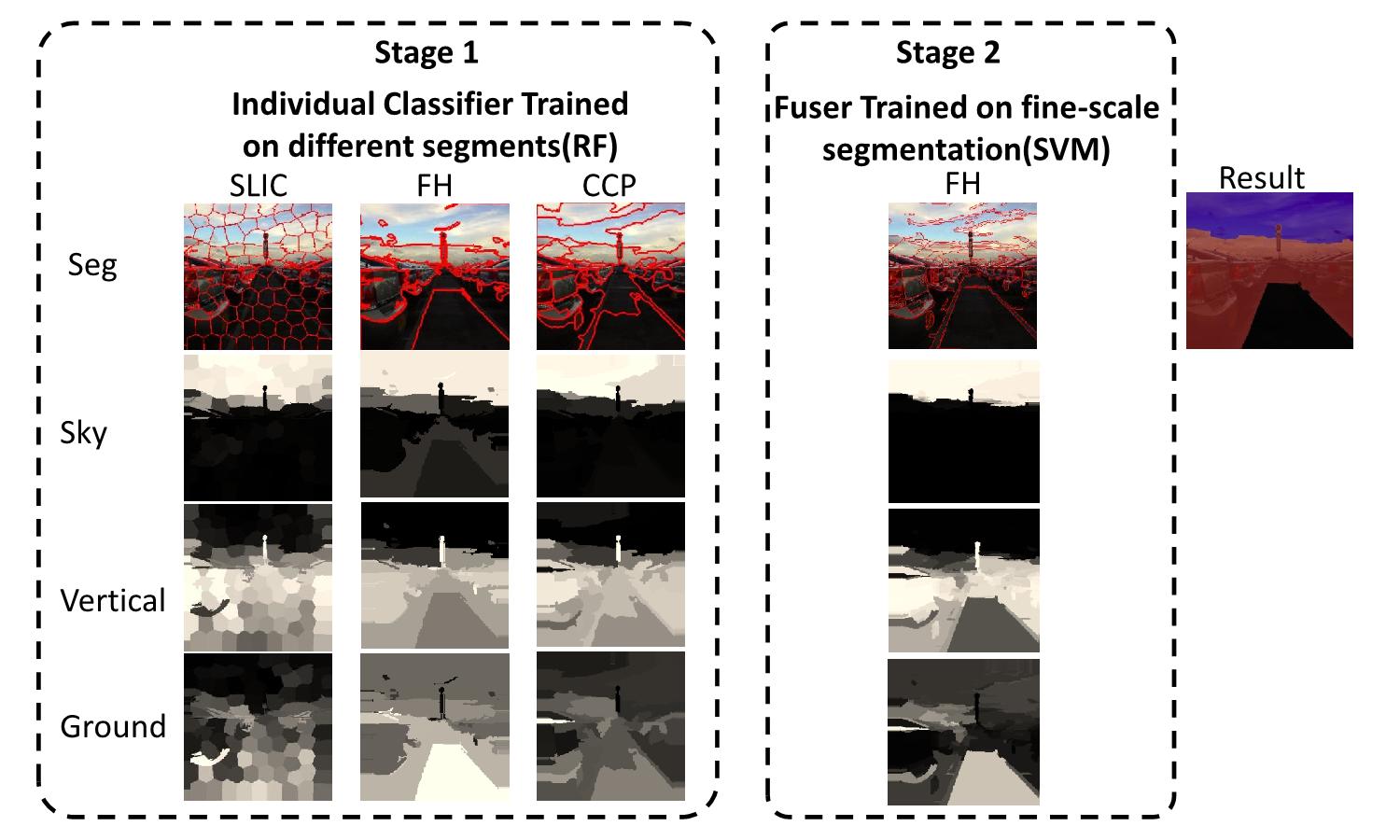
To enhance the prediction accuracy for sky and support in [16], we develop a 3-class labeling scheme that classifies pixels to three major classes; namely, “support”, “vertical” and “sky”, where planar left/right/center, porous and solid are merged into one “vertical” mega-class. This 3-class classifier is achieved by integrating segmentation results from SLIC [35], FH [34], and CCP [36] with a random forest classifier [37] in a two-stage classification system. Figure2 shows the proposed two-stage system. In the first stage, we train individual classifiers for “support”,“vertical” and “sky” and get their probability maps using the SLIC, FH and CCP segmentations. In the second stage, since the segmentation units are not the same, we transfer all segments into smaller segmentation units using the FH method to obtain the fine-scale segmentation boundaries. Then, we fuse the probability output from the first stage to get the final decision.

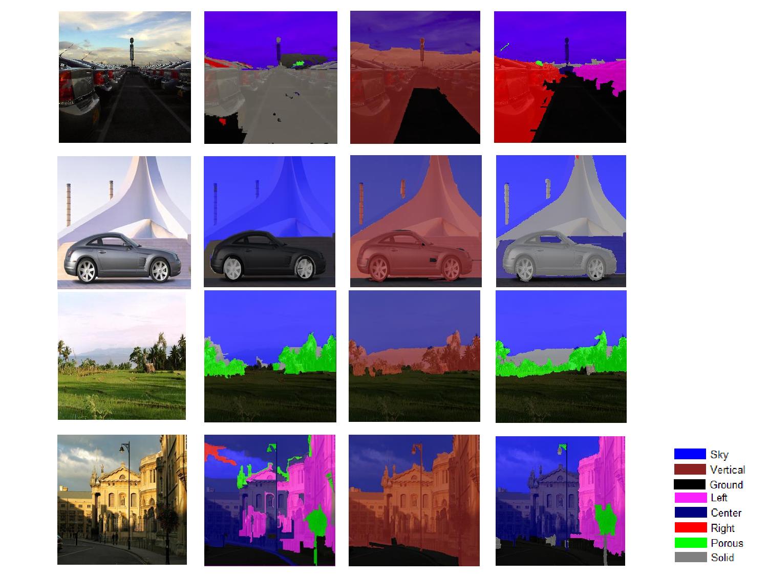
The reason of combining different segmentation schemes is that different segmentation methods capture different levels of information. For example, the SLIC method [35] provides more segments in the “support” region than the FH and CCP methods in the first stage. Thus, the SLIC segmentation has better location information and a higher chance to get the correct result for “support”. The performance of our 3-class labeling scheme is 88.7%, which is better than that of [16] by 2%. Several visual comparisons are shown in Figure3. We see that our 3-class labeling system can segment the low contrast “support” and “sky” well. After the 3-class labeling, initial labels of the five classes inside the vertical region come directly from [16].

The accuracy of the IPL stage is highly impacted by three factors: 1) a small number of training samples, 2) the weak discriminant power of local features, and 3) lacking of a global scene structure. They are common challenges encountered by all machine learning methods relying on local features with a discriminative model. To overcome these challenges, we design global attributes vectors and integrate them into a graphical model, which is elaborated in the next subsection.

Figure 2: Fusion of 3-class labeling algorithms. Stage 1: Three individual random forest classifiers trained by segments from SLIC [35], FH [34] and CCP [36], respectively, where the gray images show the probability output of each individual classifier under different segmentation methods and different geometric classes. Stage 2: The three probability outputs from Stage 1 are cascaded into one long feature vector for each intersected segmentation unit and an SVM classifier is trained to get the final decision.

Figure 3: Comparison of initial pixel labeling results (from left to right): the original image, the 7-class labeling result from [16], the proposed 3-class labeling result, the ground truth 7-class labeling. Our scheme offers better “support” and “sky” labels.

III-C Global Attributes Extraction (GAE)

In the second GAE stage, we attempt to fill out the 7D binary-valued GAV and find the related information associated with an existing element. The 7 global attributes are: 1) the sky/ground line, 2) the horizon, 3) the planar surface, 4) the vertical line, 5) the vanishing line, 6) the solid object, and 7) the porous material. Take image $I$ with dimension $H\times W\times 3$ as an example. In the GAE stage, its 7D GAV will be extracted to generate 7 probability maps denoted by $P_{k}$, $k=1,\cdots,7$, where the dimension of $P_{k}$ is $H\times W$ and $k$ represents one of the 7 global attributes. Furthermore, we use $P_{k}(s_{i},l_{j})$ to denote the probability for segment $s_{i}$ to be labeled as $l_{j}$, where $j$ denotes one of the 7 classes (support, left, center, right, porous, solid and sky) based on global attribute $k$.

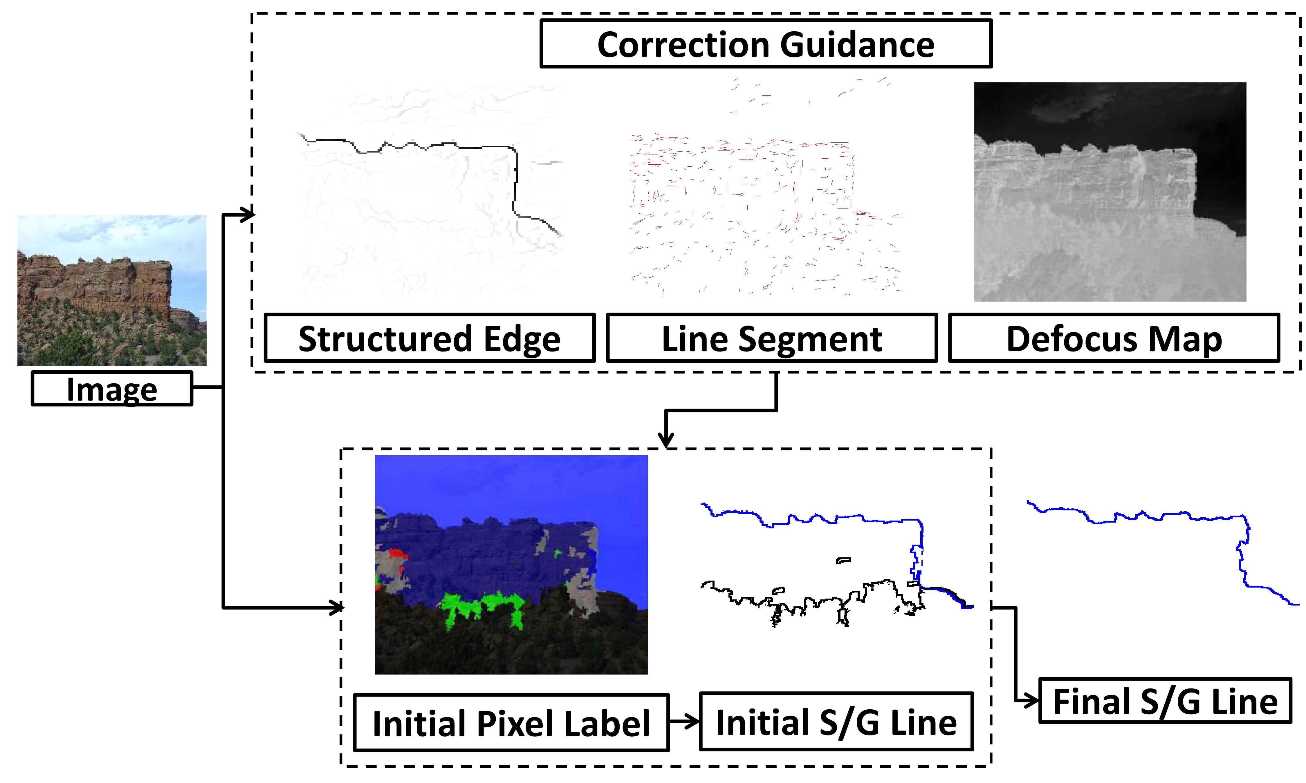
Sky and Ground Lines Detection. Sky and ground regions are important ingredients of the geometrical layout of both natural and urban scenes. To infer their existence and correct locations is critical to the task of scene understanding. We develop a robust procedure to achieve this goal as illustrated in Figure4. Based on initial pixel labels obtained in the first stage, we obtain initial sky and ground lines, which may not be correct due to erroneous initial labels.

To finetune initial sky and ground lines, we exploit the following three cues from the input scene image for sky and ground line validation:

• the line segment map denoted by $P_{LS}$ [38], where $P_{LS}=1$ for line pixels, $P_{LS}=0$ for non-line pixels;

• the probability edge map of structured edges denoted by $P_{SE}$, [39], [40], [41]; and

• the probability edge map of the defocus map denoted by $P_{DF}$ [42].

The final probability is defined as

$$P_{\text{sky/ground line}}(s_{i},l_{\text{sky/ground}})=P_{LS}\times P_{SE}\times P_{DF}.$$ (1)

An example is given in Figure4, where all three maps have higher probability for the sky line but lower probability scores for the ground line. As a result, the erroneous ground line is removed.

After obtaining the sky and ground lines, we check whether there is any vertical region above the sky line or below the ground line using the 3-class labeling scheme, where the vertical region is either solid or porous. The new 3-class labeling scheme can capture small vertical regions well and, after that, we will zoom into each vertical region to refine its subclass label.

Figure 4: The process of validating the existence of the sky/ground lines and their location inference.

Horizon Detection. When the ground plane and the sky plane meet, we see a horizon. This occurs in ocean scenes or scenes with a flat ground. The horizon location helps reason the ground plane, vertical plane and the sky plane. For example, the ground should not be above the horizon while the sky should not be below the horizon. Generally speaking, 3D layout estimation accuracy can be significantly enhanced if the ground truth horizon is available for layout reasoning[16]. Research on horizon estimation from building images was done before, e.g., [43], [44]. That is, it can be inferred by connecting horizontal vanishing points. However, the same technique does not apply to natural scene images where the vanishing point information is lacking.

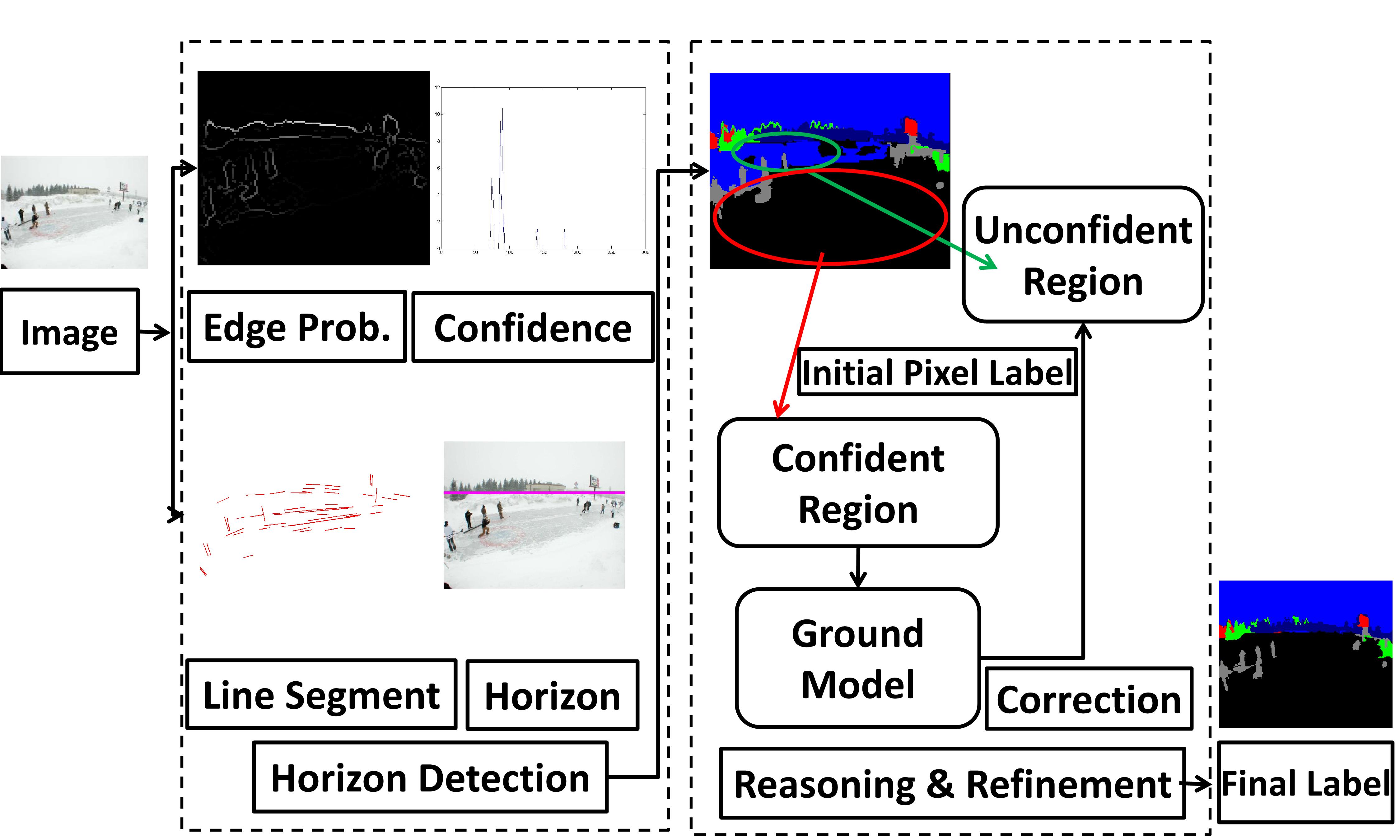
In our implementation, we use two different methods to estimate the horizon in two different outdoor scenes. For images containing buildings as evidenced by strong vertical line segments, their horizon can be estimated by fitting the horizontal vanishing points[44]. For natural scene images that do not have obvious vanishing points, we propose a horizon estimation algorithm as shown in Figure5. First, we extract multiple horizontal line segments from the input image using the LSD algorithm [38]. Besides, we obtain the edge probability map based on [39], [40], [41] and use it as well as a location prior to assign a probability to each pixel in the line segments. Then, we build a histogram to indicate the probability of the horizon location. Finally, we will select the most likely horizonal line to be the horizon.

After detecting the horizon, we perform layout reasoning to determine the sky and support regions. One illustrative example is given in Figure5. We can divide the initial labeled segments into two regions. If a segment above (or below) the horizon is labeled as sky (or support), it belongs to the confident region. On the other hand, if a segment above (or below) the horizon is labeled as support (or sky), it belongs to the unconfident region. The green circled region in Figure5 is labeled as sky due to its white color. Thus, it lies in the unconfident region. There exists a conflict between the local and global decisions. To resolve the conflict, we use the Gaussian Mixture Model (GMM) to represent the color distribution in the confident region above and below the horizon. Then, we conclude that the white color under the horizon can actually be the support (or ground) so that its label can be corrected accordingly. We use $P_{\text{horizon}}(s_{i},l_{j})$ to denote the probability output from the GMM.

Figure 5: Horizon detection and its application to layout reasoning and label refinement.

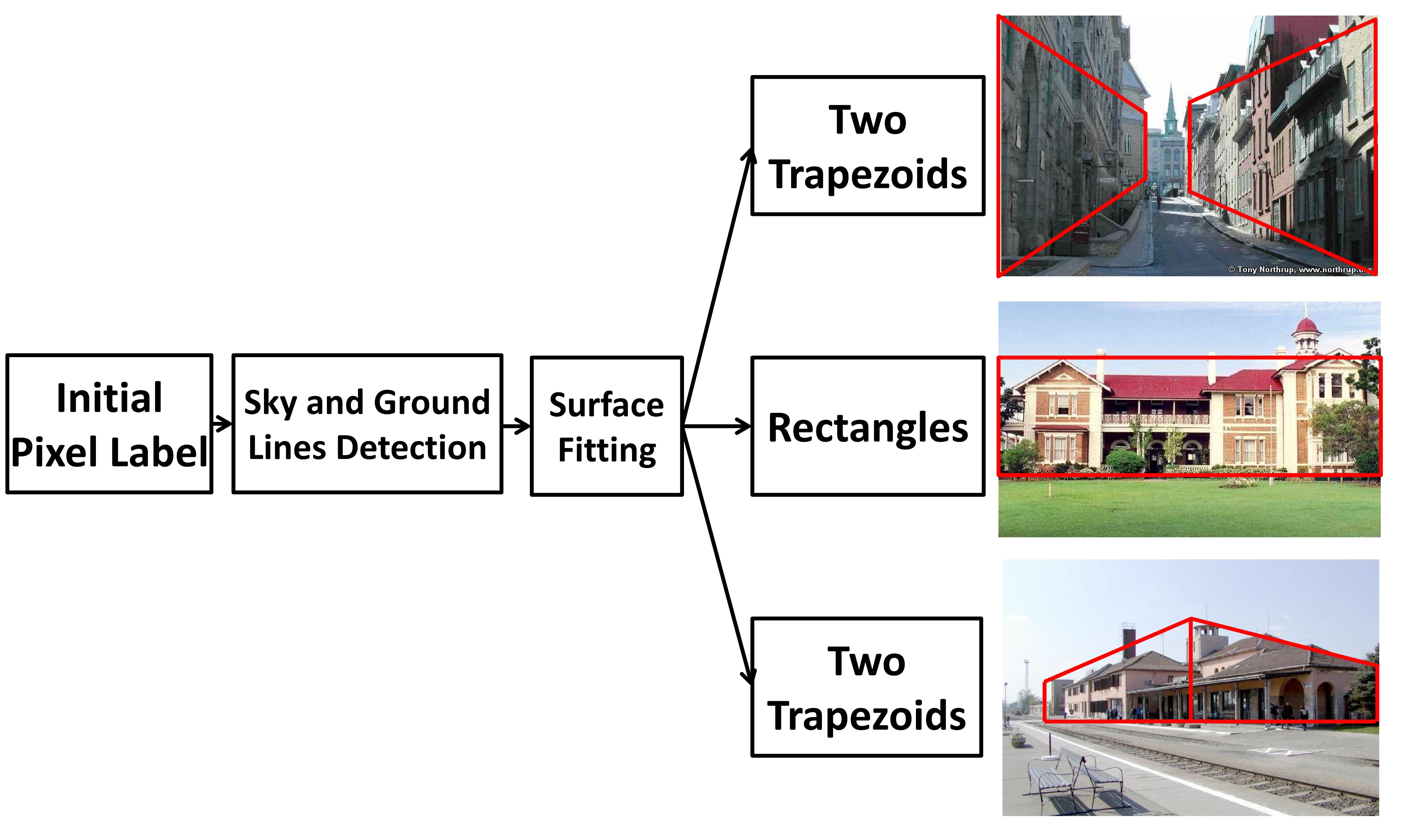
Planar Surfaces Detection. An important by-product of sky/ground line localization is the determination of planar surface orientation in the vertical region. This is feasible since the shapes of sky and ground lines provide useful cues for planar surface orientation inference in natural or urban scenes. To be more specific, we check the trapezoidal shape fitting scheme (including triangles and rectangles as special cases) for the vertical region, where the top and the bottom of the trapezoidal shape are bounded by the sky and ground lines while its left and right are bounded by two parallel vertical lines or extends to the image boundary. We set $P_{\text{planar surface}}(s_{i},l_{j})=1$, where $j\in{\text{(left,center,right)}}$, if the corresponding surface orientation is detected. Otherwise, we set $P_{\text{planar surface}}(s_{i},l_{j})=0$.

Three trapezoidal region shape fitting examples are shown in Figure6. Clearly, different fitting shapes indicate different planar surface orientations. For example, two trapezoidal regions with narrow farther sides indicate an alley scene as shown in the top example. A rectangle shape indicates a front shot of a building as shown in the middle example. The two trapezoidal regions with one common long near side indicates two building facades with different orientations as given in the bottom example. Thus, the shapes of sky and ground lines offer important cues to planar surface orientations.

Figure 6: Trapezoidal shape fitting with the sky line in the top and the ground line in the bottom.

Vertical Line Detection. A group of parallel vertical line segments provides a strong indicator of a building structure in scene images. It offers a valuable cue in correcting wrongly labeled regions in building scene images. The probability of surface orientation from the vertical line is denoted by $P_{\text{verticall}}(s_{i},l_{j})$, where $j\in{\text{(left, center, right)}}$. In our implementation, we use the vertical line percentage in a region as the attribute to generate the probability map for the building region. An example of using vertical lines to correct wrongly labeled regions is illustrated in Figure7. The top region of the building is wrongly labeled as “sky” because of the strong location and color cues in the initial labeling result. However, the same region has a strong vertical line structure. Since the “sky” region should not have this structure, we can correct its wrong label.

Figure 7: An example of vertical line detection and correction.

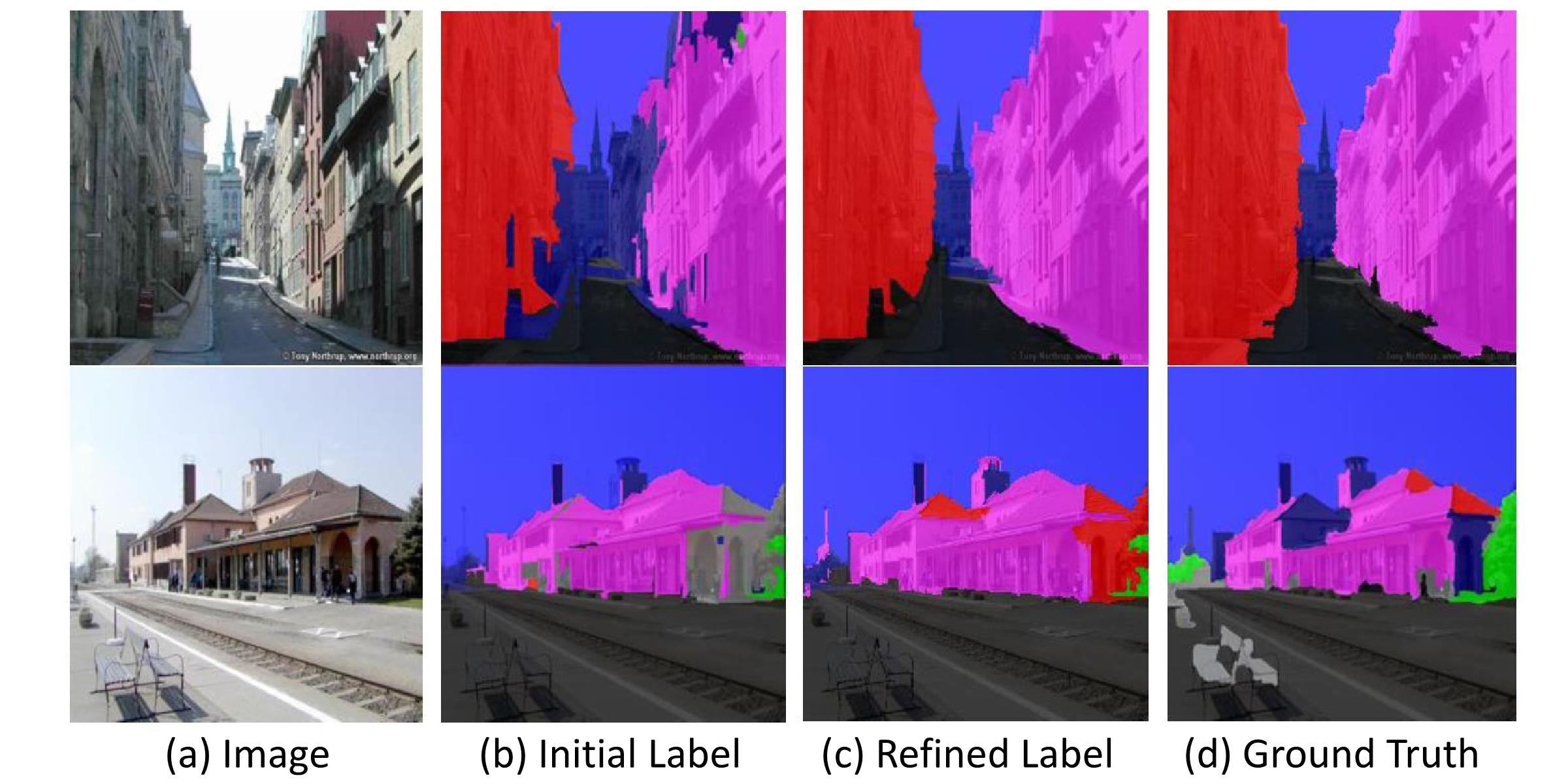
Vanishing Line Detection. A group of vanishing lines offers another global attribute to indicate the surface orientation. In our implementation, we first use the vertical line detection technique to obtain a rough estimate of the left and right boundaries of a building region and then obtain its top and bottom boundaries using the sky line and the ground line. After that, we apply the vanishing line detection algorithm in [3] and use the obtained vanishing line result to adjust the orientation of a building facade. We set $P_{\text{vanishingl}}(s_{i},l_{j})=1$, where $j\in{\text{(left,center,right)}}$, if the corresponding surface orientation is detected. Otherwise, we set $P_{\text{vanishingl}}(s_{i},l_{j})=0$. Note that the surface orientation of a planar surface can be obtained from its shape and/or vanishing lines. If it is not a building, we cannot observe vanishing lines and the shape is the only cue. If it is a building we can observe both its shape and vanishing lines. The two cues are consistent with each other based on our experience. Two examples of using the shape and vanishing lines of a building region to correct erroneous initial labels are given in Figure8. The initial surface orientation provided by the IPL stage contains a large amount of errors due to the lack of global view. They are corrected using the global attributes.

Figure 8: Examples of surface orientation refinement using the shape and the vanishing line cues.

Solid Detection. The non-planar solid class is typically composed by foreground objects (such as people, car, etc.) rather than the background scene. The bottom of an object either touches the ground or extends to the image bottom boundary. For example, objects (say, pedestrians and cars) may stand on the ground in front of the building facade in an urban scene while objects are surrounded by the ground plane in a typical natural scene. Object detection is an active research field by itself. Actually, the object size has an influence on the scene content, i.e. whether it is an object-centric or scene-centric image. The object size is big in an object-centric image. It occupies a large portion of the image, and most of the background is occluded. The scene layout problem is of less interest since the focus is on the object rather than the background. In contrast, there is no dominant object in a scene-centric image and the scene layout problem is more significant. On one hand, it is better to treat the object detection problem independently from scene analysis. On the other hand, a scene image may still contain some objects while the background scene is occluded by them. For examples, the existence of objects may occlude some part of sky and ground lines, thus increasing the complexity of scene layout estimation. In order to simplify the scene understanding problem, it is desired to identify and remove objects first.

In our implementation, we apply two object detectors (namely, the person detector and the car detector) from [45] [46]. We first obtain the bounding boxes of detected objects and, then, adopt the grab cut method [47] to get their exact contours. The grab cut method uses a binary value to indicate whether a pixel belong to object or not. Mathematically, we have $P_{\text{solid}}(s_{i},l_{\text{solid}})=1$ for the location where solid is detected, and $P_{\text{solid}}=0$, otherwise. Two examples are shown in Figure9. To achieve a better layout estimation, detected and segmented objects are removed from the scene image to allow more reliable sky and ground line detection.

Figure 9: Examples of obtaining the object mask using the person and the car object detectors and the grab cut segmentation method: (a) the bounding boxes result of the person detector, (b) the person segmentation result, (c) the bounding box result of the car detector, and (d) the car segmentation result.

Figure 10: Two examples of initially labeled porous regions where the top (trees) is correctly labeled while the bottom (mountain) is wrongly labeled.

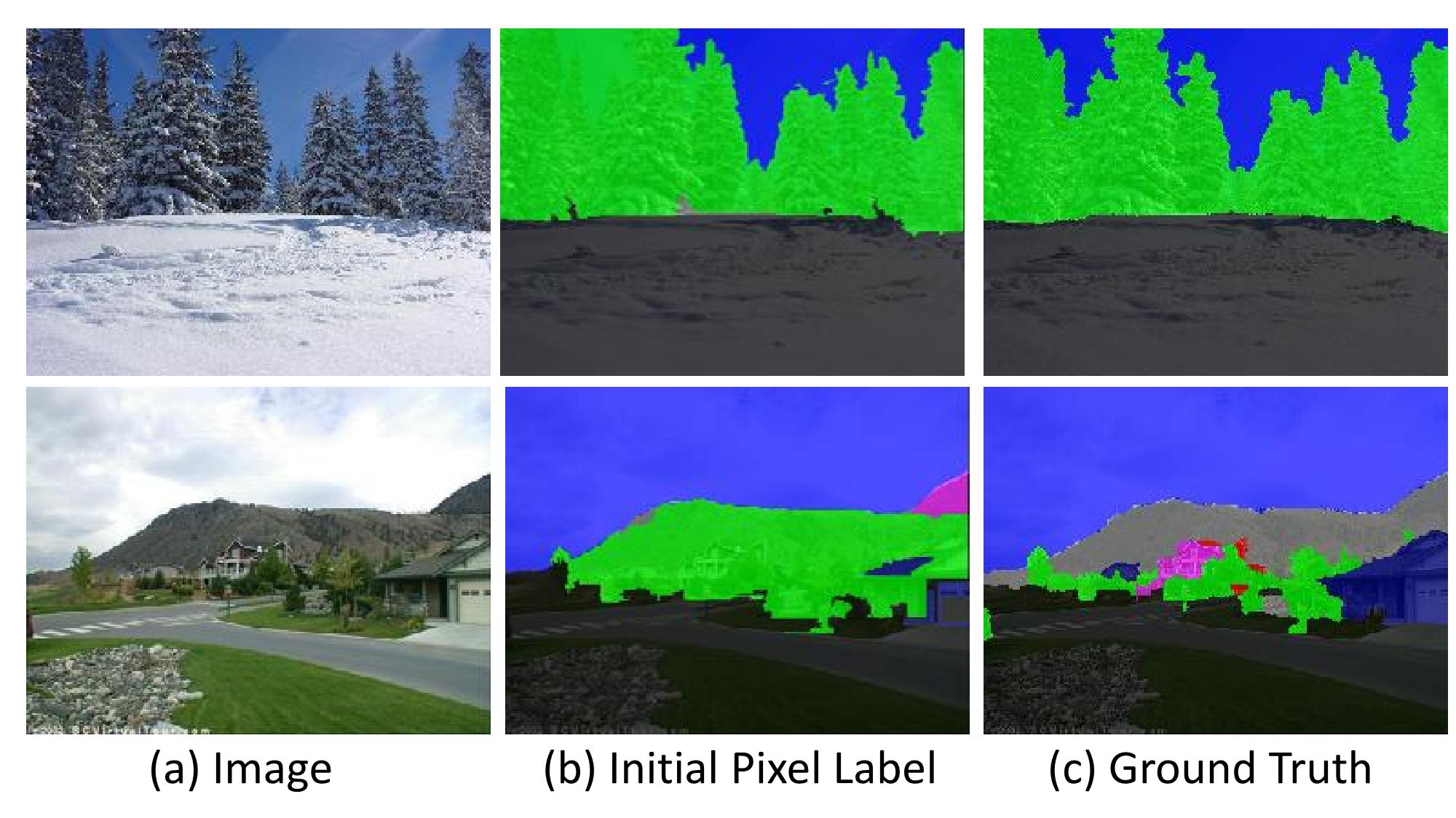
Porous Detection. As shown in the bottom subfigure of Figure10, the mountain region, which belongs to the solid class, is labeled as porous by mistake. This is due to the fact that the super-pixel segmentation method often merges the porous region with its background. Thus, it is difficult to split them in the classification stage. To overcome this difficulty, we add the contour randomness feature from the structured edge result [39], [40], [41] to separate the porous and the solid regions. Note that $P_{\text{porous}}(s_{i},l_{\text{porous}})$ is proportional to contour randomness. By comparing the two examples in Figure10, we see that there exist irregular contours inside the true porous region (trees) but regular contours inside the solid region (mountain). In our implementation, we double check regions labeled by solid or porous initially and use the contour smoothness/randomness to separate solid/porous regions.

III-D Layout Reasoning and Label Refinement (LR2)

The 7D GAV can characterize a wide range of scene images. In this section, we focus on layout reasoning using the extracted global attribute vector. We first analyze the outdoor scenes from the simplest setting to the general setting as shown in Figure11. Then, we propose a Conditional Random Field (CRF) minimization framework for outdoor layout reasoning.

Figure 11: A proposed framework for geometric layout reasoning: (a) the simplest case, (b) the background scene only, and (c) a general scene, where SL, GL, H, O denote the sky line, the ground line, the horizon and the occluder, respectively.

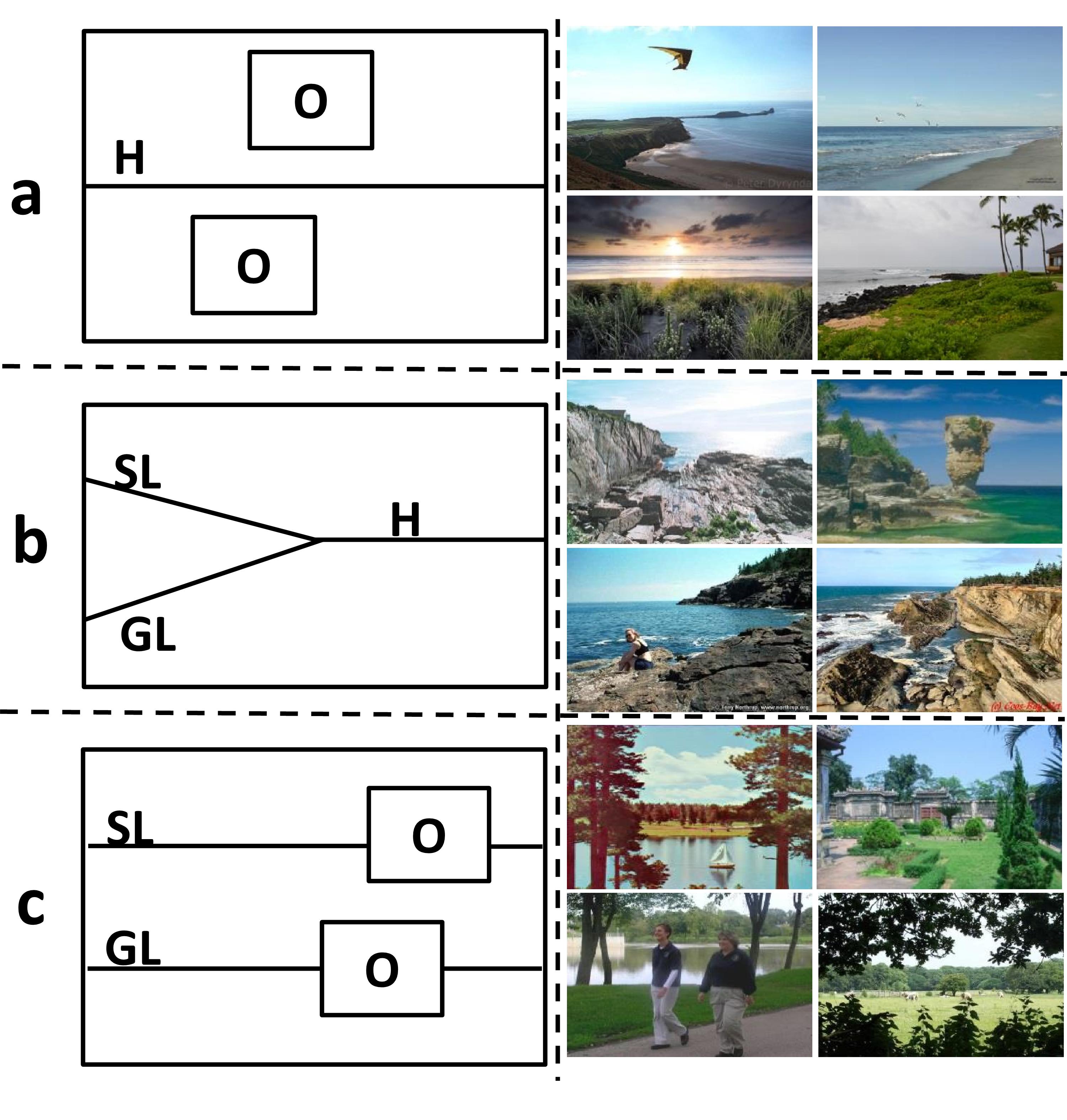
The simplest case of our interest is a scene with a horizon as shown in Figure11(a). This leads to sky and support two regions and the support could be ocean or ground. The existence of occluders makes this case slightly more complicated. The sky may have two occluders - solid (e.g., balloon, bird, airplane, kite, parashoot) and porous (e.g., tree leaves near the camera). The ocean/ground may also have occluders - solid (e.g, boat in the ocean, fence/wall near the camera) and porous (e.g. bushes near the camera). Although there are rich scene varieties, our layout reasoning framework can remove segments labeled with planar center/left/right in the simplest case confidently.

The horizon will be split into individual sky and ground lines if there exist large planar surfaces that completely or partially block the horizon as shown in Figure11(b). It is a background scene only, if there is no occluder. The large planar surfaces can be buildings in urban scenes and mountains in natural scenes. Generally speaking, any region between the sky and ground lines is a strong candidate for planar surfaces. We can further classify them into planar left/right/center based on vanishing lines or the outer contour of the surface region. A general scene may have all kinds of solid/porous occluders (e.g. people, car, trees, etc.) in front of a background scene as shown in Figure11(c). The occluders may block the ground line, the planar surface and other solid/porous objects to make layout inference very challenging. In the following, we exploit initial pixel labeling and all attributes and formulate layout reasoning as a Conditional Random Field (CRF) [48], [49] optimization problem.

Problem Formulation: We model each image as a graph denoted by $G(S,E)$, where each node is the super-pixel segment and a member of $S$ and two adjacent vertices are connected by an edge which is a member of $E$. Our goal is to minimize the following energy function given the adjacency graph $G(S,E)$ and a weight $\lambda$:

$$E(\mathbf{L}) =\sum_{s_{i}\in S}\Psi(l_{i}|s_{i})+\lambda\sum_{(s_{i},s_{j})\in E}\Phi(l_{i},l_{j}|s_{i},s_{j}),$$ (2)

where $S$ is the segmentation of consideration, $l_{i}$ is the class label assigned to the $i^{th}$ segment $s_{i}$, $\Psi$ is the unary potential function, $\Phi$ is the pairwise potential function, and $\lambda$ is a tradeoff between the unary potential and the pairwise potential. Empirically, we set $\lambda=0.1$.

We classify the seven proposed global attributes into two major groups. The first group consists of the horizon, the vertical line, the solid and the porous. Their probability maps are determined by the appearance properties of segments rather than the context relationship among adjacent segments. It is proper to adopt the unary potential as their probability outputs. The second group consists of the sky/ground line, the vanishing line, the left or right-oriented surfaces, which describe the relationship among adjacent segments. Thus, we consider the pairwise potential of these attributes. Specifically, we have the following definitions of the unary potential and the pairwise potential.

We define the unary potential for each segment $s_{i}$ as

$$\Psi(l_{i}|s_{i})=-\log(P(l_{i}|s_{i})),$$ (3)

where

$$P(l_{i}|s_{i})={\textbf{w}^{\intercal}}\left(\begin{array}[]{c}P_{\text{initial}}(l_{i}|s_{i})\\ P_{\text{porous}}(l_{i}|s_{i})\\ P_{\text{solid}}(l_{i}|s_{i})\\ P_{\text{horizon}}(l_{i}|s_{i})\\ P_{\text{verticall}}(l_{i}|s_{i})\\ \end{array}\right)$$ (4)

is the probability that segment $s_{i}$ is predicted with label $l_{i}$. In words, probability $P(l_{i}|s_{i})$ is the weighted average of five components: 1) initial label probability $P_{\text{initial}}(l_{i}|s_{i})$ which comes from the label probability from our 3 class classifier and vertical class classifier from [50]; 2) porous detector $P_{\text{porous}}(l_{i}|s_{i})$; 3) solid detector $P_{\text{solid}}(l_{i}|s_{i})$; 4) horizon line inference $P_{\text{horizon}}(l_{i}|s_{i})$; and 5) vertical line inference $P_{\text{verticall}}(l_{i}|s_{i})$. The weight vector w is a 5D vector that determines the contributions of the five components in the unary potential.

We define the pairwise potential for pairwise segments $s_{i}$ and $s_{j}$ as

$$\Phi(l_{i},l_{j}|s_{i},s_{j})=(\Phi_{s}+\Phi_{v}+\Phi_{p})[l_{i}\neq l_{j}],$$ (5)

where $[\cdot]$ is a zero-one indicator function and

$$\Phi_{s}=-\log(P_{\text{sky/ground line}_{\text{b}}}(s_{i},s_{j})),$$ (6)

$$\Phi_{v}=-\log(\|P_{\text{vanishing line}}(s_{i},l_{i})-P_{\text{vanishing line}}(s_{j},l_{j})\|),$$ (7)

$$\Phi_{p}=-\log(\|P_{\text{planar surfance}}(s_{i},l_{i})-P_{\text{planar surface}}(s_{j},l_{j})\|)$$ (8)

where $P_{\text{sky/ground line}_{\text{b}}}(s_{i},s_{j})$, $P_{\text{vanishing line}}(s_{i},l_{i})$, and $P_{\text{planar surfance}}(s_{i},l_{i})$ denote averaged probability along the shared boundary of $s_{i}$ and $s_{j}$, probability of $s_{i}$ is labeled as $l_{i}$ from vanishing line information, and probability of $s_{i}$ is labeled as $l_{i}$ from planar surface information, respectively, and $\|\cdot\|$ is the norm of the probability difference between segments $s_{i}$ and $s_{j}$.

In Eq. 6, when there is neither sky nor ground line across $s_{i}$ and $s_{j}$, $P_{\text{sky/ground line}_{\text{b}}}(s_{i},s_{j})$ should be small. However, $\Phi_{s}$ would be large if $s_{i}$ and $s_{j}$ are with different labels. To minimize potential function in Eq. 2, $\Phi_{s}$ forces $s_{i}$ and $s_{j}$ to be with the same label. This explains how the ground line is removed in the example given in Fig. 4. Furthermore, $\Phi_{v}$ and $\Phi_{p}$ are the pairwise potentials computed from the probability map of vanishing lines and the probability map of planar surface orientation as shown in Eqs. 7 and 8, respectively. A smoothness constraint is imposed by $\Phi_{v}$ (or $\Phi_{p}$). $\Phi_{v}$ (or $\Phi_{p}$) penalizes more if $s_{i}$ and $s_{j}$ have different labels yet their vanishing line (or planar surface orientation) difference at location $s_{i}$ and $s_{j}$ is small. This explains how the surface orientation smoothness can be achieved in the examples given in Figure8.

We first learn the parameters, w and $\lambda$, from the CRF model by maximizing their conditional likelihood through cross-validation on the training data. Then, the multi-label graph cut optimization method [48] is used to minimize the energy function in Eq. 2.

IV Experimental Results

In contrast to the object detection problem, very few datasets are available for geometric layout algorithms evaluation. The dataset in [16] is the largest benchmarking dataset in the geometric layout research community. There are larger geometric layout datasets but for indoor images which doesn’t fit our problem [1], [3]. The dataset in [16] consists of 300 images of outdoor scenes with labeled ground truth. The first 50 images are used for training the surface segmentation algorithm as done in previous work [16], [22]. The remaining 250 images are used for evaluation. We follow the same procedure in our experiments. To test our generalized global attributes and reasoning system, we use the same 250 testing images in our experiment.

It is not a straightforward task to label the ground truth for outdoor scene images in this dataset. It demands subjects to reason the functionalities of different surfaces in the 3D real world (rather than recognizing objects in images only), e.g., where is the occlusion boundary? what is the surface orientation? whether there is depth difference? etc. To get a consistent ground truth, subjects should be very well trained. Note that we do not agree with the labeled ground truth of several images, and will report them in the supplemental material. In this section, we will present both qualitative and quantitative evaluation results and analyze several poorly labeled images.

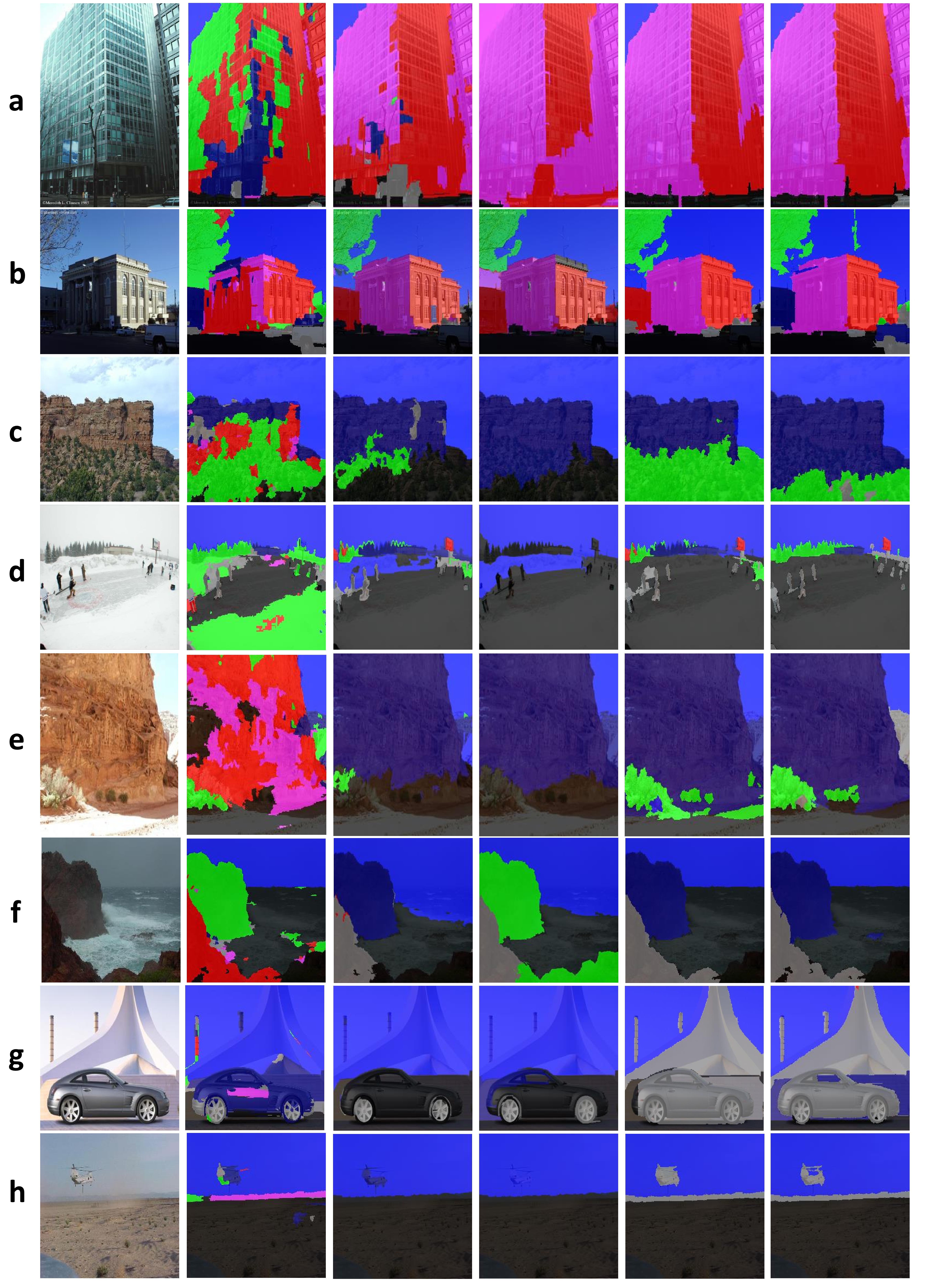
Qualitative Analysis. Figure12 shows eight representative images (the first column) with their labeled ground truths (the last column). We show results obtained by CNN method [27](the second column), Hoiem et al. [16] (the third column), Gupta et al. [22] (the fourth column), the proposed GAL (the fifth column). To apply the CNN to this problem, we retrained the CNN use the training data with initialized weights from the VGG network [27]. We call the methods proposed in Hoiem et al. [16] and Gupta et al. [22] the H-method and the G-method, respectively, in the following discussion for convenience.

In Figure12 (a), the building is tilted and its facade contains multiple surfaces with different orientations. Because of the similarity of the local visual pattern (color and texture), the CNN method got confused between surface and porous. The H-method is confused by upper and lower parts in the planar-left facade, and assigns them to planar left and right two opposite oriented surfaces. This error can be corrected by the global attribute (ie building’s vertical lines). The G-method loses the detail of surface orientation in the upper left corner so that the sky and the building surface are combined into one single planar left surface. It also loses the ground support region. These two errors can be corrected by sky-line and ground-line detection. GAL infers rich semantic information about the image from the 7D GAV. Both the sky and the ground exist in the image. Furthermore, it is a building facade due to the existence of parallel vertical lines. It has two strong left and right vanishing points so that it has two oriented surfaces - one planar left and the other planar right. There is a problem remaining in the intersection region of multiple buildings in the right part of the image. Even humans may not have an agreement on the number of buildings in that area (two, three, or four?) The ground truth also looks strange. It demands more unambiguous global information for scene layout inference.

For Figure12 (b), the ground truth has two problems. One is in the left part of the image. It appears to be more reasonable to label the building facade to “planar left” rather than “planar center”. Another is in the truck car region. The whole truck should have the same label; namely, gray (non-planar solid). This example demonstrates the challenging nature of the geometric layout problem. Even human can make mistakes easily. Other observed human-labeling mistakes in ground truth are reported in the supplemental file.

Figure12 (c)-(f) show the benefit of getting an accurate sky line and/or an accurate ground line. One powerful technique to find the sky line and the ground line is to use defocus estimation. Once these two lines are detected, the inference becomes easier so that GAL yields better results.

Being constrained by the limited model hypothesis, the G-method chooses to have the ground (rather than the porous) to support the physical world. However, this model does not apply to the image in (c), images with bushes in the bottom as an occluder, etc. Also, the ground truth in (c) is not consistent in the lower region. The result obtained by GAL appears to be more reasonable.

Figure12 (d) was discussed earlier. Both the H-method and the G-method labeled part of the ground as the sky by mistake due to color similarity. GAL can fix this problem using horizon line detection. All three methods work well for Figure12 (e). GAL performs slightly better due to the use of the horizon detection and label refinement stage. The right part of the image is too blurred to be of interest. GAL outperforms the CNN-method, the H-method and the G-method due to an accurate horizon detection in Figure12 (f). Figure12 (g) demonstrates the power of the sky line detection and object (car) detector. Figure12 (h) demonstrates the importance of an accurate sky line detection.

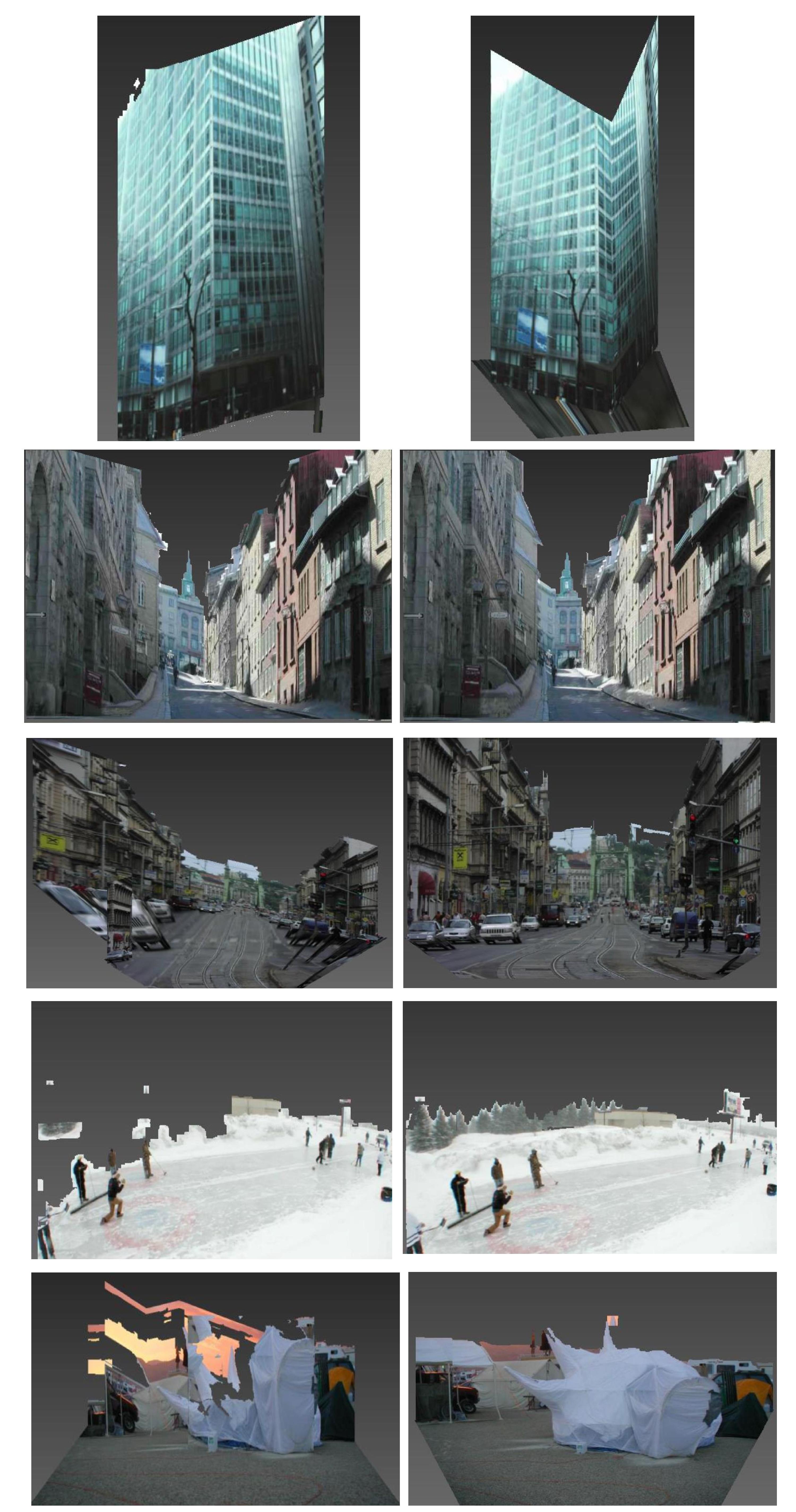
We also compare the “pop-up” view of the H-method and GAL in Figure13 using a 3D view rendering technique given in [2], [17]. It is clear that GAL offers a more meaningful result.

Figure 12: Qualitative comparisons of three geometric layout algorithms (from left to right): the original Image, CNN-method[27], Hoiem et al. [16], Gupta et al. [22], the GAL and the ground truth. The surface layout color codes are magenta (planar left), dark blue (planar center), red (planar right), green (non-planar porous), gray (non-planar solid), light blue (sky), black (support).

Based on the above discussion, we can draw several concluding points. First, there are not enough examples for the CNN to learn the visual pattern. The CNN is a data driven approach that extract visual patterns from training data. For the geometric labeling problem, labels cannot be fully determined by visual patterns. For example, the left and right surface of a building have similar color and texture visual pattern locally, but their orientations are different. In contrast, the orientation can be captured by the global information such as shapes and lines. With very little training data, CNN’s power is somehow limited. Second, the local-patch-based machine learning algorithm (e.g., the H-method) lacks the global information for 3D layout reasoning. It is difficult to develop complete outdoor scene models to cover a wide diversity of outdoor images (e.g., the G-method). GAL attempts to find key global attributes from each outdoor image. As long as these global attributes can be determined accurately, we can combine the local properties (in form of initial labels) and global attributes for layout reasoning and label refinement. Third, the proposed methodology can handle a wider range of image content. As illustrated above, it can provide more satisfactory results to quite a few difficult cases that confuses prior art such as the H-method and the G-method.

Figure 13: Comparison of 3D rendered views based on geometric labels from the H-method (left) and GAL (right).

Quantitative Analysis. For quantitative performance evaluation, we use the metric used in [17, 22] by computing the percentage of overlapping of labeled pixel and ground truth pixel (called the pixel-wise labeling accuracy). We use the original ground truth given in [50] for fair comparison between all experimental results reported below (with only one exception which will be clearly stated).

Figure 14: Comparison of labeling accuracy between the CNN methods, the H-method, the G-method and GAL with respect to seven individual labels.

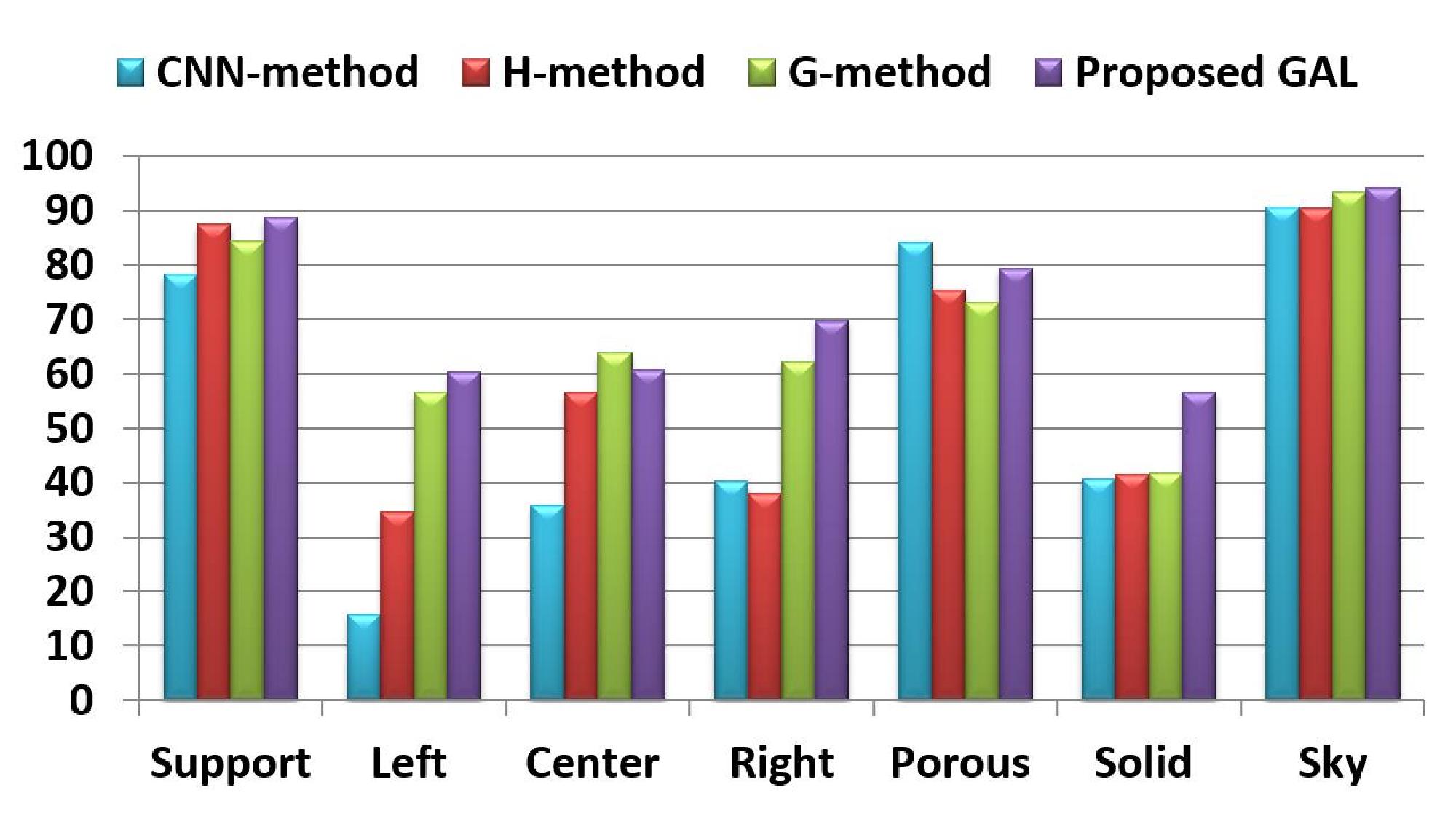
We first compare the labeling accuracy of the CNN-method, the H-method, the G-method and GAL for seven geometric classes individually in Figure14. We see clearly that GAL outperforms the H-method in all seven classes by a significant margin. The gain ranges from 1.27% (support) to more than 25% (planar left and right). GAL also outperforms the G-method in 6 classes. The gain ranges from 0.81% (sky) to 14.9% (solid). The G-method and GAL have comparable performance with respect to the “planar center” class. All methods do well in sky and ground labeling. The solid class is the most challenging one among all seven classes since it has few common geometric structures to exploit.

The complete performance benchmarking (in terms of pixel-wise labeling accuracy) of five different methods are shown in Table I. The L-method in [24] and the P-method in [25] were dedicated to building facade labeling and their performance were only evaluated on subsets of the full dataset in [50]. The L-method in [24] use the subset which contains 100 images images where the ground truth of both occlusion boundaries and surface orientation are provided [16]. P-method in [25] use the subset which contains 55 building images.

We use B1, B2, F and F/R to denote the subset used in [24], the subset used in [25], the full dataset and the full dataset with relabeled ground truth in the table, respectively. The two numbers within the parenthesis (7 and 5) denote results for all “seven” classes and for the “five” vertical classes (i.e., excluding sky and support), respectively. For the F(7) column in Table I, we compare the performance for all seven classes in the full set. Accurate labeling for this dataset is actually very challenging as pointed out in [51], [52]. This is also evidenced by the slow performance improvement over the last seven years - a gain of 2.35% from the H-method to the G-method. GAL offers another gain of 4.95% over the G-method [22], which is significant. For the B1(5) column, we compare the performance for five classes in the building subset which contains 100 images. GAL outperforms the CNN-method and the L-method by 21.24% and 3.39%, respectively. For the B2(7) column, we compare the performance against the building subset which contains 55 images. GAL outperforms the CNN-method, the H-method, the G-method and the P-method by 20.4%, 8.8%, 8.08% and 6.85%, respectively. For the F(5) column, we compare the performance for five classes in the full set. GAL outperforms the CNN-method, the H-method, the G-method by 19.64%, 7.14% and 2.22%. Finally, for the F/R(7) column, we show the labeling accuracy of GAL against the modified ground truth. The labeling accuracy can go up to 80.26%.

TABLE I: Comparison of the averaged labeling accuracy (%) of six methods with respect to the building subset (B), the full set (F) and the full set with relabeled ground truth (F/R), where 7 and 5 mean all seven classes and the five classes belonging to the vertical category, respectively.Results are updated

	Dataset (Class No.)
	B1(5)	B2(7)	F(5)	F(7)	​F/R(7)​
CNN-method [27]	58.33	61.27	56.33	68.21	N/A
H-method [16]	N/A	72.87	68.80	72.41	N/A
G-method [22]	N/A	73.59	73.72	74.76	N/A
L-method [24]	76.34	N/A	N/A	N/A	N/A
P-method [25]	N/A	74.82	N/A	N/A	N/A
Proposed GAL	79.73	81.67	75.94	79.71	80.26

To further analyze the performance gain of proposed GAL system, we add the global attributes one by one to our proposed GAL system and analyze performance gain from individual global attribute, which is shown in Table.2. The initial result for 7 class tested in the full set is 74.88% which is obtained by our 3 class labeling result and the labels in vertical region from [50]. When compute the performance gain from global attribute horizon, $P_{\text{horizon}}$ is first computed and $P_{\text{horizon}}$ is included in the unary term in CRF model. As there is no global attributes contribute to pairwise term, we simply apply the same pairwise edge potentials defined in [48]. As both attribute planar surface and attribute vanishing line contribute to surface orientation accuracy improvement, we include both of them to see their performance gain together. The table shows that all global attributes contributes to the performance gain significantly.

TABLE II: The performance gain from each individual attribute.

	porous	solid	horizon
Performance Gain	+0.12%	+ 0.80%	+ 1.08%
	vertical	sky/ground	vanishing line
	line	line	planar surface
Performance Gain	+ 1.00%	+ 0.48%	+ 0.95%

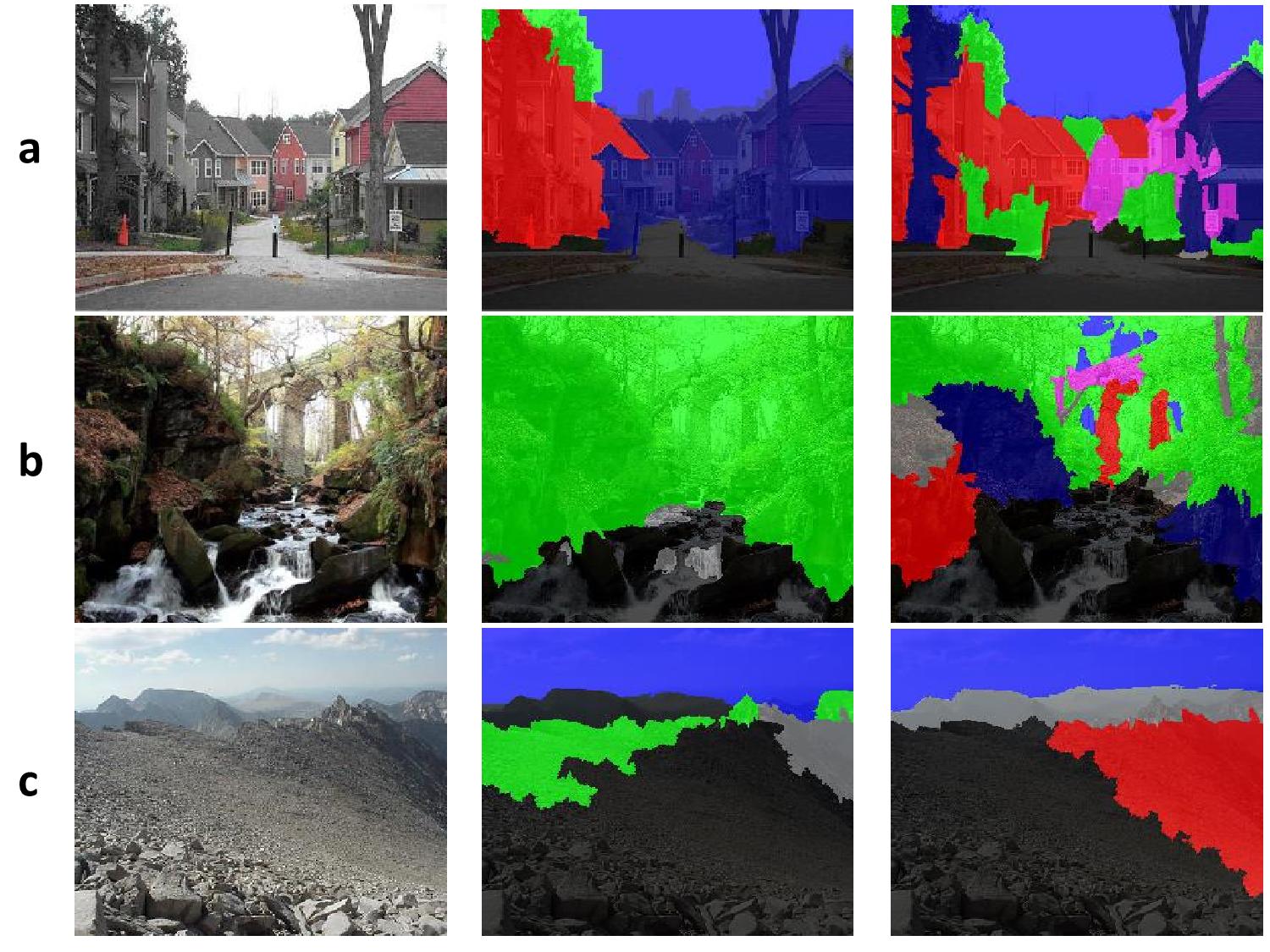
Error Analysis. Three exemplary images that have large labeling errors are shown in Figure15. Figure15 (a) is difficult due to the complexity in the middle region of multiple houses. We feel that the labeled “planar center” result by GAL for this region is still reasonable although it is not as refined as that offered by the ground truth. Figure15 (b) is one of the most challenging scenes in the dataset since even humans may have disagreement. The current ground truth appears to be too complicated to be useful. GAL can find the ground line but not the sky line due to the tree texture in the top part of the image. GAL made a labeling mistake in porous in Figure15 (c) due to dominant texture in the corresponding region. We need a better porous detector to fix this problem. The global attributes will not be able to help much. There is a planar right region in the ground truth. Although this label is accurate to human eyes by looking at the local surface, the transition from support (or ground) to planar right is not natural. It could be an alternative to treat the whole region in the bottom part as support. As shown in this image, it is extremely difficult to find an exhaustive set of scene models to fit all different situations.

Figure 15: Error analysis of the proposed GAL system with three exemplary images (one example per row and from left to right): the original image, the labeled result of GAL and the ground truth.

V Conclusion

A novel GAL geometric layout labeling system for outdoor scene images was proposed in this work. GAL exploits both local and global attributes to achieve higher accuracy and it offers a major advancement in solving this challenging problem. Its performance was analyzed both qualitatively and quantitatively. Besides, several error cases were studied to reveal the limitations of the proposed GAL system.

Clearly, there are still many interesting problems remaining, including the development of better global attributes extraction tools, its integration with CNN detectors, and the design of more powerful and more general inference rules. Furthermore, due to major differences between indoor and outdoor scene images, the key global attributes of indoor scene images will be different from those of outdoor scene images. So, more research needs to be done to develop a GAL system for indoor scenes. Future research is planned to determine important global attributes of indoor scene images and to study their geometric layout.

References

- [1] W. Choi, Y.-W. Chao, C. Pantofaru, and S. Savarese, “Understanding indoor scenes using 3d geometric phrases,” in Proceedings of the IEEE Conference on Computer Vision and Pattern Recognition, 2013, pp. 33–40.
- [2] D. Hoiem, A. A. Efros, and M. Hebert, “Automatic photo pop-up,” ACM Transactions on Graphics (TOG), vol. 24, no. 3, pp. 577–584, 2005.
- [3] V. Hedau, D. Hoiem, and D. Forsyth, “Recovering the spatial layout of cluttered rooms,” in Computer vision, 2009 IEEE 12th international conference on. IEEE, 2009, pp. 1849–1856.
- [4] A. Gupta, S. Satkin, A. Efros, and M. Hebert, “From 3d scene geometry to human workspace,” in Computer Vision and Pattern Recognition (CVPR), 2011 IEEE Conference on. IEEE, 2011, pp. 1961–1968.
- [5] H. Mobahi, Z. Zhou, A. Y. Yang, and Y. Ma, “Holistic 3d reconstruction of urban structures from low-rank textures,” in Computer Vision Workshops (ICCV Workshops), 2011 IEEE International Conference on. IEEE, 2011, pp. 593–600.
- [6] S. Park, H. Lee, S. Lee, and H. S. Yang, “Line-based single view 3d reconstruction in manhattan world for augmented reality,” in Proceedings of the 14th ACM SIGGRAPH International Conference on Virtual Reality Continuum and its Applications in Industry. ACM, 2015, pp. 89–92.
- [7] B. Liu, S. Gould, and D. Koller, “Single image depth estimation from predicted semantic labels,” in Computer Vision and Pattern Recognition (CVPR), 2010 IEEE Conference on. IEEE, 2010, pp. 1253–1260.
- [8] D. Eigen, C. Puhrsch, and R. Fergus, “Depth map prediction from a single image using a multi-scale deep network,” in Advances in neural information processing systems, 2014, pp. 2366–2374.
- [9] L. Ladicky, J. Shi, and M. Pollefeys, “Pulling things out of perspective,” in Proceedings of the IEEE Conference on Computer Vision and Pattern Recognition, 2014, pp. 89–96.
- [10] J. Zou, W. Li, C. Chen, and Q. Du, “Scene classification using local and global features with collaborative representation fusion,” Information Sciences, vol. 348, pp. 209–226, 2016.
- [11] M. Zang, D. Wen, K. Wang, T. Liu, and W. Song, “A novel topic feature for image scene classification,” Neurocomputing, vol. 148, pp. 467–476, 2015.
- [12] C. Chen, Y. Ren, and C.-C. J. Kuo, “Outdoor scene classification using labeled segments,” in Big Visual Data Analysis. Springer, 2016, pp. 65–92.
- [13] C. Gururaj, D. Jayadevappa, and S. Tunga, “An effective implementation of exudate extraction from fundus images of the eye for a content based image retrieval system through hardware description language,” in Emerging Research in Computing, Information, Communication and Applications. Springer, 2016, pp. 279–290.
- [14] J. Johnson, R. Krishna, M. Stark, L.-J. Li, D. A. Shamma, M. S. Bernstein, and L. Fei-Fei, “Image retrieval using scene graphs,” in Computer Vision and Pattern Recognition (CVPR), 2015 IEEE Conference on. IEEE, 2015, pp. 3668–3678.
- [15] M. Paulin, M. Douze, Z. Harchaoui, J. Mairal, F. Perronin, and C. Schmid, “Local convolutional features with unsupervised training for image retrieval,” in Proceedings of the IEEE International Conference on Computer Vision, 2015, pp. 91–99.
- [16] D. Hoiem, A. Efros, and M. Hebert, “Closing the loop in scene interpretation,” in Computer Vision and Pattern Recognition, 2008. CVPR 2008. IEEE Conference on. IEEE, 2008, pp. 1–8.
- [17] D. Hoiem, A. A. Efros, and M. Hebert, “Recovering surface layout from an image,” International Journal of Computer Vision, vol. 75, no. 1, pp. 151–172, 2007.
- [18] P. Koutsourakis, L. Simon, O. Teboul, G. Tziritas, and N. Paragios, “Single view reconstruction using shape grammars for urban environments,” in Computer Vision, 2009 IEEE 12th International Conference on. IEEE, 2009, pp. 1795–1802.
- [19] D. C. Lee, M. Hebert, and T. Kanade, “Geometric reasoning for single image structure recovery,” in Computer Vision and Pattern Recognition, 2009. CVPR 2009. IEEE Conference on. IEEE, 2009, pp. 2136–2143.
- [20] A. Saxena, M. Sun, and A. Y. Ng, “Make3d: Learning 3d scene structure from a single still image,” Pattern Analysis and Machine Intelligence, IEEE Transactions on, vol. 31, no. 5, pp. 824–840, 2009.
- [21] W. Choi, Y.-W. Chao, C. Pantofaru, and S. Savarese, “Understanding indoor scenes using 3d geometric phrases,” in Computer Vision and Pattern Recognition (CVPR), 2013 IEEE Conference on. IEEE, 2013, pp. 33–40.
- [22] A. Gupta, A. A. Efros, and M. Hebert, Blocks world revisited: Image understanding using qualitative geometry and mechanics, ser. Computer Vision–ECCV 2010. Springer, 2010, pp. 482–496.
- [23] A. Gupta, M. Hebert, T. Kanade, and D. M. Blei, “Estimating spatial layout of rooms using volumetric reasoning about objects and surfaces,” in Advances in Neural Information Processing Systems, 2010, pp. 1288–1296.
- [24] X. Liu, Y. Zhao, and S.-C. Zhu, “Single-view 3d scene parsing by attributed grammar,” in Computer Vision and Pattern Recognition (CVPR), 2014 IEEE Conference on. IEEE, 2014, pp. 684–691.
- [25] J. Pan, M. Hebert, and T. Kanade, “Inferring 3d layout of building facades from a single image,” in Proceedings of the IEEE Conference on Computer Vision and Pattern Recognition, 2015, pp. 2918–2926.
- [26] J. Long, E. Shelhamer, and T. Darrell, “Fully convolutional networks for semantic segmentation,” in Proceedings of the IEEE Conference on Computer Vision and Pattern Recognition, 2015, pp. 3431–3440.
- [27] V. Badrinarayanan, A. Kendall, and R. Cipolla, “Segnet: A deep convolutional encoder-decoder architecture for image segmentation,” arXiv preprint arXiv:1511.00561, 2015.
- [28] S. Zheng, S. Jayasumana, B. Romera-Paredes, V. Vineet, Z. Su, D. Du, C. Huang, and P. H. Torr, “Conditional random fields as recurrent neural networks,” in Proceedings of the IEEE International Conference on Computer Vision, 2015, pp. 1529–1537.
- [29] C. Farabet, C. Couprie, L. Najman, and Y. LeCun, “Learning hierarchical features for scene labeling,” Pattern Analysis and Machine Intelligence, IEEE Transactions on, vol. 35, no. 8, pp. 1915–1929, 2013.
- [30] P. H. Pinheiro and R. Collobert, “Recurrent convolutional neural networks for scene parsing,” arXiv preprint arXiv:1306.2795, 2013.
- [31] D. J. Im, C. D. Kim, H. Jiang, and R. Memisevic, “Generating images with recurrent adversarial networks,” arXiv preprint arXiv:1602.05110, 2016.
- [32] H. Noh, S. Hong, and B. Han, “Learning deconvolution network for semantic segmentation,” in Proceedings of the IEEE International Conference on Computer Vision, 2015, pp. 1520–1528.
- [33] J. Dai, K. He, and J. Sun, “Instance-aware semantic segmentation via multi-task network cascades,” arXiv preprint arXiv:1512.04412, 2015.
- [34] P. F. Felzenszwalb and D. P. Huttenlocher, “Efficient graph-based image segmentation,” International Journal of Computer Vision, vol. 59, no. 2, pp. 167–181, 2004.
- [35] R. Achanta, A. Shaji, K. Smith, A. Lucchi, P. Fua, and S. Susstrunk, “Slic superpixels compared to state-of-the-art superpixel methods,” Pattern Analysis and Machine Intelligence, IEEE Transactions on, vol. 34, no. 11, pp. 2274–2282, 2012.
- [36] X. Fu, C.-Y. Wang, C. Chen, C. Wang, and C.-C. Jay Kuo, “Robust image segmentation using contour-guided color palettes,” in Proceedings of the IEEE International Conference on Computer Vision, 2015, pp. 1618–1625.
- [37] A. Liaw and M. Wiener, “Classification and regression by randomforest,” R news, vol. 2, no. 3, pp. 18–22, 2002.
- [38] R. G. von Gioi, J. Jakubowicz, J.-M. Morel, and G. Randall, “Lsd: A fast line segment detector with a false detection control,” IEEE Transactions on Pattern Analysis & Machine Intelligence, no. 4, pp. 722–732, 2008.
- [39] P. Dollár and C. L. Zitnick, “Fast edge detection using structured forests,” 2014.
- [40] C. L. Zitnick and P. Dollár, “Edge boxes: Locating object proposals from edges,” in Computer Vision–ECCV 2014. Springer, 2014, pp. 391–405.
- [41] P. Dollár and C. L. Zitnick, “Structured forests for fast edge detection,” in Computer Vision (ICCV), 2013 IEEE International Conference on. IEEE, 2013, pp. 1841–1848.
- [42] S. Zhuo and T. Sim, “Defocus map estimation from a single image,” Pattern Recogn., vol. 44, no. 9, pp. 1852–1858, Sep. 2011.
- [43] F. Han and S.-C. Zhu, “Bottom-up/top-down image parsing with attribute grammar,” Pattern Analysis and Machine Intelligence, IEEE Transactions on, vol. 31, no. 1, pp. 59–73, 2009.
- [44] O. Barinova, V. Lempitsky, E. Tretiak, and P. Kohli, Geometric image parsing in man-made environments, ser. Computer Vision–ECCV 2010. Springer, 2010, pp. 57–70.
- [45] R. B. Girshick, P. F. Felzenszwalb, and D. McAllester, “Discriminatively trained deformable part models, release 5,” http://people.cs.uchicago.edu/ rbg/latent-release5/.
- [46] P. F. Felzenszwalb, R. B. Girshick, D. McAllester, and D. Ramanan, “Object detection with discriminatively trained part-based models,” Pattern Analysis and Machine Intelligence, IEEE Transactions on, vol. 32, no. 9, pp. 1627–1645, 2010.
- [47] C. Rother, V. Kolmogorov, and A. Blake, “Grabcut: Interactive foreground extraction using iterated graph cuts,” ACM Transactions on Graphics (TOG), vol. 23, no. 3, pp. 309–314, 2004.
- [48] B. Fulkerson, A. Vedaldi, S. Soatto et al., “Class segmentation and object localization with superpixel neighborhoods.” in ICCV, vol. 9. Citeseer, 2009, pp. 670–677.
- [49] D. Song, W. Liu, T. Zhou, D. Tao, and D. A. Meyer, “Efficient robust conditional random fields,” Image Processing, IEEE Transactions on, vol. 24, no. 10, pp. 3124–3136, 2015.
- [50] D. Hoiem, A. Efros, M. Hebert et al., “Geometric context from a single image,” in Computer Vision, 2005. ICCV 2005. Tenth IEEE International Conference on, vol. 1. IEEE, 2005, pp. 654–661.
- [51] S. Lazebnik and M. Raginsky, “An empirical bayes approach to contextual region classification,” in Computer Vision and Pattern Recognition, 2009. CVPR 2009. IEEE Conference on. IEEE, 2009, pp. 2380–2387.
- [52] S. Ramalingam, P. Kohli, K. Alahari, and P. H. Torr, “Exact inference in multi-label crfs with higher order cliques,” in Computer Vision and Pattern Recognition, 2008. CVPR 2008. IEEE Conference on. IEEE, 2008, pp. 1–8.