Statistical QoS Analysis of Full Duplex and Half Duplex Heterogeneous Cellular Networks

Abstract

In this paper, statistical Quality of Service provisioning in next generation heterogeneous mobile cellular networks is investigated. To this aim, any active entity of the cellular network is regarded as a queuing system, whose statistical QoS requirements depend on the specific application. In this context, by quantifying the performance in terms of effective capacity, we introduce a lower bound for the system performance that facilitates an efficient analysis. We exploit this analytical framework to give insights about the possible improvement of the statistical QoS experienced by the users if the current heterogeneous cellular network architecture migrates from a Half Duplex to a Full Duplex mode of operation. Numerical results and analysis are provided, where the network is modeled as a Matérn point processes with a hard core distance. The results demonstrate the accuracy and computational efficiency of the proposed scheme, especially in large scale wireless systems.

I Introduction

The ever increasing demand for mobile data traffic continues with the advent of smart phones, tablets, mobile routers, and cellular M2M devices. This is accompanied by user behavioral changes from web browsing towards video streaming, social networking, and online gaming with distinct QoS requirements [1]. To handle this challenging scenario, researchers are examining different enabling technologies for 5G, including mmWave communications for wider bandwidth, extreme densification of the network via low power base stations (known as heterogenous networks), the use of large–scale antenna systems (known as Massive MIMO), and wireless Full Duplex entities [2].

The new cellular architecture known as Heterogeneous Cellular Networks (HCNs) refers to a scenario in which the macro cellular network is overlaid by heterogeneous low–power base stations (BSs). Such low power BSs have small coverage areas and are characterized by their own transmit power and named accordingly as micro, pico and femto cells. They are used to increase the capacity of the network while eliminating coverage holes [3].

The Full Duplex (FD) radio technology enhances spectrum efficiency by enabling a node to transmit and receive in the same frequency band at the same time. This new emerging technology has the potential to double the physical layer capacity and enhance the performance even more, when higher layer protocols are redesigned accordingly [4].

Due to the hurdles of canceling self–interference (SI) in FD devices via active and passive suppression mechanisms, FD operations are more reliable in low power wireless nodes. For instance in [5] the authors have implemented an FD WiFi radio operating in an unlicensed frequency band with 20 dBm transmit power while the same trend is followed in other works like [6] where the maximum transmit power is 15 dBm. All these implementations suggest FD technology as a very good candidate to be used in the low power BSs deployed within HCNs. Moreover, the increased spectral efficiency of the FD systems, combined with that of HCNs, provides another strong motivation in attempting to analyze an FD HCN.

From another perspective, next generation mobile networks (5G) will aim not only to increase the network capacity but also to enhance several other performance metrics, including lower latency, seamless connectivity, and increased mobility [2]. These enhancements can be generally referred to as an improvement in the Quality of Service (QoS) experienced by the network entities. According to a forecast by Ericsson mobility report, approximately 55 percent of all the mobile data traffic in 2020 will account for mobile video traffic while another 15 percent will account for social networking [1]. These multimedia services require a bounded delay. Generally the delay requirements of time sensitive services in 5G will vary extremely, from milliseconds to a few seconds [7]. Consequently, the analysis of statistical QoS in HCNs will become extremely important in the near future.

The objective of this paper is to analyze and compare FD and HD HCNs in provisioning statistical QoS guarantees to the users in the network. The QoS is assessed statistically in terms of Effective Capacity (EC) as the maximum throughput under a delay constraint [8].

Our goal is to provide insights on possible improvements in the QoS experience of end users if the current architecture migrates from conventional HD to FD. To this end, we propose a lower bound for the EC which greatly reduces the complexity of the analysis while tightly approximating the system performance, especially in large scale systems. Our results will be validated through numerical simulations.

The rest of the paper is organized as follows. Some basic explanations on FD, statistical QoS provisioning, and stochastic geometry are provided in Section II. The system model is described in Section III. Section IV presents the proposed lower bound for the system performance and the corresponding theoretical analysis, whose results are validated through simulations in Section V. Finally, Section VI concludes this paper.

II Preliminaries

II-A Full Duplex

In–band Full Duplex (IBFD) devices are capable of transmitting and receiving data in the same frequency band at the same time. In traditional wireless terminals, the ratio of SI power with respect to that of the received intended signal is very high, making any reception infeasible while a transmission is ongoing. To overcome this issue, FD terminals are equipped with active and passive cancellation mechanisms to suppress their own SI in the received signal [4]. However, in practice, because of the many imperfections in transceiver operations, full cancellation of the SI signal is not possible. Therefore, some residual self–interference (RSI) always remains after all cancellation steps and results in a degraded system performance.

The RSI signal represents the main obstacle for a perfect FD communication and, similar to noise, is essentially uncorrelated with the original transmitted signal. We model the RSI signal at the FD transceiver as a complex Gaussian random variable [9]

$$\mathrm{RSI}\sim\mathbb{CN}\left({0,\eta{P^{\kappa}}}\right),$$ (1)

where $P$ is the transmit power, while $\eta$ and $\kappa$ are parameters to model the SI cancellation performance. Specifically, $\eta$ is the linear SI cancellation parameter, while $\kappa$ models non–linear SI cancellation, $0\leq\eta,\kappa\leq 1$. When no SI cancellation is performed $\eta,\kappa=1$, while $\eta=0$ represents the ideal case of perfect SI cancellation.

II-B Statistical QoS guarantees

Real–time multimedia services like video streaming require bounded delays. In this context, a received packet that violates its delay bound requirement is considered useless and discarded. Due to the wireless nature of the access links in a mobile cellular network, providing deterministic delay bound guarantees is not possible. Thus, the concept of EC, defined as the maximum throughput under a given delay constraint, has been used to analyze multimedia wireless systems [10]. Any active entity in a cellular network can be regarded as a queueing system: it generates packets according to an arrival process, stores them in a queue and transmits them according to a service process. For stationary and ergodic arrival and service processes, the probability that the queue size, $Q$, exceeds a certain threshold, $B$, decays exponentially fast as the threshold increases [10], i.e.,

$$\Pr\left\{{Q>B}\right\}\sim{e^{-\theta B}}\qquad\textrm{as}\,B\rightarrow\infty,$$ (2)

where $\theta$ denotes the decaying rate of the QoS violation probability. The smaller $\theta$, the looser the QoS requirement.

Define the service provided by the channel until time slot $t$ as

$$C\left({0,t}\right)=\sum\limits_{k=1}^{t}{R\left[k\right]},$$ (3)

where $R[k]$ denotes the number of bits served in time slot $k$. The effective capacity of the channel is defined as [8]

$${\rm{EC}}\left(\theta\right)=-\frac{{{\Lambda_{C}}\left({-\theta}\right)}}{\theta}$$ (4)

where $\Lambda_{C}\left(-\theta\right)=\lim\limits_{t\to\infty}\frac{1}{t}\log\operatorname{\mathbb{E}}\left\{e^{-\theta C(0,t)}\right\}$ is the Gärtner - Ellis limit of the service process $C(0,t)$.

If the instantaneous service process, $R[k]$, is independent in time, EC can be simplified to

$${\rm{EC}}\left(\theta\right)=-\frac{1}{\theta}\log{\operatorname{\mathbb{E}}\left\{{{e^{-\theta R[k]}}}\right\}}$$ (5)

It is worth mentioning that, for $\theta\rightarrow 0$, the EC tends to the average service rate [10].

II-C Stochastic Geometry

Stochastic geometry is a powerful mathematical tool that has recently been proposed to model and analyze the performance of wireless networks [11]. In particular, Poisson Point Processes (PPPs) have been vastly used to model the positions of the network entities in HCNs. This approach has enabled the study of realistic scenarios where the BSs are not placed on a hexagonal grid but are instead spread randomly in the network. The use of a PPP to model the system has become popular because of its tractability and its ability to give simple expressions for some network performance metrics like coverage probabilities and mean transmission rates [11], [12], and [13]. However, in a real cellular network, the adoption of a simple PPP to model the locations of the BSs does not capture an important characteristic of the network, namely the constraints on the minimum distance between any two BSs or UEs imposed by the MAC layer, network planning or spectrum access policies [11]. Consequently, spatial correlation among different network entities should be taken into account. According to these considerations, a repulsive point process with a hard core distance such as the Matérn hard core point process (HCPP), despite its higher complexity, represents a better candidate to model a HCN compared to a simple PPP [11].

III System Model

We refer to Fig. 1 as our system model in both HD and FD scenarios. When the system is HD a conventional HCN is assumed, while in the FD case we consider a completely FD HCN where all the network entities are assumed to be (imperfect) FD devices. In our model we consider a circular macro cell, overlaid by different tiers of small cells, each with its own characteristics including transmit power, path loss exponent, and coverage range. Each tier is assumed to have a circular coverage area provided by an omnidirectional antenna to serve any user within its coverage range.

In addition, we assume a Matérn Point Process with hard core distance to model the location of non–overlapping small cells and the distribution of the user equipments (UEs) within each small cell. In our FD HCN system model, the nodes communicate in bidirectional FD mode, as depicted in Fig. 1. The small cells are assumed to use out of band resources like fiber optics, wire, or microwave links for backhauling.

In our analysis, we assume that the positions of the BSs are known by the network operator. This assumption is not far from reality since, when the network operator wants to give service to a BS, the location of the BS must be communicated to the operator. The locations of the users of each BS are assumed to be uniformly distributed in the coverage area of that BS, resulting in a Matérn PP but with known locations for the cluster heads.

In the FD scenario, a UE in the network experiences three different types of interference: (1) RSI, due to concurrent transmission and reception in the same frequency band at the same time; (2) interference from BSs that are transmitting in the same resource blocks (RBs) in which the UE is served; and (3) interference from other UEs in the network that are transmitting in the same RBs in which the UE is served. In an HD scenario, instead, the UE will not face RSI and interference from other UEs. However, the interference from other BSs will still be present and can be even greater than in the FD case, according to the adopted scheduling policy. To consider the worst case, in both the FD and HD scenarios, we have assumed that all the BSs in the network are transmitting in the same RB where the UE is served.

We analyze the system on a resource block basis. In fact the scheduling decisions in an LTE–Advanced cellular network are made on a 1 ms basis and each time the scheduler in the BS grants an arbitrary combination of 180 kHz $\times$ 0.5 ms wide RBs to a UE based on the Buffer Status Report (BSR) and Channel State Information (CSI) obtained by measuring the reference signals in both time and frequency [14]. This allows the scheduler to track the variations of the channel in time and frequency in order to schedule resources efficiently.

Figure 1: System model: an HCN with one macrocell and several LPNs.

III-A Interference from UEs and BSs

We consider a Rayleigh fading, path loss dominated, AWGN channel model. With this model, the interference at the desired UE from another entity of the network located at distance $x$ is given by $Ph{\left\|x\right\|^{-\alpha}}$ where $P$ is transmit power of the interferer, $h$ is an exponential random variable modeling Rayleigh fading, $h\sim\exp\left(1\right)$, and $\alpha$ represents the path loss exponent.

Considering all the above mentioned terms, the Signal–to–Interference plus Noise Ratio (SINR) at the desired FD UE is expressed as [12]

$$\textrm{SINR}=\frac{{{P_{i}}{h_{{x_{i}}}}{\left\|x_{i}\right\|}{{}^{-\alpha_{i}}}}}{{\sum\limits_{k}{\sum\limits_{x\in{\Phi_{k}^{\textrm{BS}}}}{{P_{k}}{h_{x}}\left\|x\right\|{{}^{-{\alpha_{k}}}}}}+\sum\limits_{k}{\sum\limits_{y\in{\Phi_{k}^{\textrm{UE}}}}{{P_{\textrm{UE}}}}}{h_{y}}\left\|y\right\|{{}^{-{\alpha_{k}}}}+\eta{P^{\kappa}}+{\sigma^{2}}}}.$$

In this notation, the numerator represents the desired signal power received from a BS in the $i^{th}$ tier which serves the UE. Here, a tier defines the set of the BSs that have the same characteristics including average transmit powers, supported data rate, coverage areas, BSs density [12]. The first and second term in the denominator represent the interference from other BSs and UEs in the network operating in the same RBs as the desired UE. Specifically, $\Phi_{k}^{\textrm{BS}}$ and $\Phi_{k}^{\textrm{UE}}$ indicate sets containing the positions of all interfering BSs and UEs in the $k^{\textrm{th}}$ tier, and the summation is over all possible tiers. The third term is the RSI signal power as modeled in (1). Finally, $\sigma^{2}$ is the additive noise power.

We recall that the number of bits delivered to a UE during an interval, $T_{f}$, in a given bandwidth, $BW$, if capacity achieving modulation and coding are used, can be represented as

$$R=T_{f}\cdot BW\cdot\log_{2}\left(1+\textrm{SINR}\right)\textrm{.}$$ (7)

Therefore, the effective capacity of the desired UE based on (5) can be expressed as

$$\textrm{EC}\left(\theta\right) =-\frac{1}{\theta}\log\left(\mathbb{E}\left\{\textrm{exp}\left(-\theta\cdot T_{f}\cdot BW\cdot\log_{2}\left(1+\textrm{SINR}\right)\right)\right\}\right)$$

$$=-\frac{1}{\theta}\log\left(\mathbb{E}\left(\left(1+\textrm{SINR}\right)^{-\theta\cdot T_{f}\cdot BW\cdot\log_{2}e}\right)\right),$$ (8)

where the expectation is taken with respect to the SINR.

In an HD scenario, a 1/2 scaling factor is needed and, also, the SINR would become

$$\textrm{SINR}=\frac{{{P_{i}}{h_{{x_{i}}}}{\left\|x_{i}\right\|}{{}^{-\alpha_{i}}}}}{{\sum\limits_{k}{\sum\limits_{x\in{\Phi_{k}^{\textrm{BS}}}}{{P_{k}}{h_{x}}\left\|x\right\|{{}^{-{\alpha_{k}}}}}}+{\sigma^{2}}}}.$$ (9)

IV Theoretical analysis

We aim at computing the QoS experienced by a generic UE, that can be placed anywhere in the coverage area of its own small cell with uniform distribution. To find the exact EC in a given topology, one needs to solve (8) either through extensive simulations or by mathematical analysis. It is worth mentioning that, if there are $M$ small cells within the macro cell, the associated integrals would be in a $2M+1$ dimensional parameter space, when a worst case scenario is assumed, i.e., any other small cell and the macro cell present one active UE operating in the same RB as our desired UE. On the other hand, if a simulation approach is pursued, the length of simulations in order to achieve a given confidence level will increase at least linearly with $M$. This scaling may represent a prohibitive factor in finding the exact EC in a real scenario.

IV-A Approximating EC

Let us define a generic function $g$ of $s,I,a,$ and $\beta$ as follows

$$g(s,I)=\left(1+\frac{s}{I+a}\right)^{-\beta}.$$ (10)

This function has the same structure of the expectation argument in (8), where $s$ models the received signal power, $I$ represents the overall interference from other BSs and UEs in the network, $a$ represents the RSI and noise, and $\beta=\theta\cdot T_{f}\cdot BW\cdot\log_{2}e$. Based on this definition, the EC can be rewritten as

$$EC(\theta)=-\frac{1}{\theta}\log\left(\operatorname{\mathbb{E}}\limits_{s,I}g\left(s,I\right)\right).$$ (11)

Lemma 1.

For $0\leq\beta\leq 1$, $g$ is always a concave function of $I$.

Proof.

By assuming $s$ as a constant, taking the second derivative of $g$ with respect to $I$ leads to

$$\frac{{{\partial^{2}}g(s,I)}}{{{\partial}{I^{2}}}}=\frac{{\beta s}}{{{{\left({I+a}\right)}^{4}}}}{\left({1+\frac{s}{{I+a}}}\right)^{-\left({\beta+2}\right)}}\left({-2\left({I+a}\right)+\left({\beta-1}\right)s}\right),$$ (12)

which is negative (i.e., $g$ is a concave function of $I$) for any value of $0\leq\beta<1+\frac{2}{{\textrm{SINR}}}$. But since SINR is a random variable depending on the instantaneous values of signal power, $s$, and interference plus noise, $I+a$, we can only be sure that $g$ is always a concave function of $I$ for any $0\leq\beta\leq 1$. ∎

The concavity of $g$ helps to find a tight lower bound for the EC with greatly decreased complexity. To this end, by exploiting Jensen’s inequality, we obtain

$$EC_{\textrm{LB}}\left(\theta\right)=\frac{{-1}}{\theta}\log{\operatorname{\mathbb{E}}_{s}}\left[{{{\left({1+\frac{s}{{\bar{I}+a}}}\right)}^{-\beta}}}\right]\leq EC\left(\theta\right).$$ (13)

Here, $\bar{I}=\operatorname{\mathbb{E}}_{I}(I)$ is the average interference experienced by the UE, and the remaining expectation only applies to the desired signal power. The advantage of this lower bound is its extremely reduced computational complexity. Indeed, calculating this lower bound only requires a 1–dimensional integral with respect to the desired signal power. Therefore, the proposed bound makes this calculation scalable with the size of the network, at the possible cost of losing some precision.

It must be noted that the constraint on $\beta$, $0\leq\beta\leq 1$, imposes a constraint on $\theta$, namely

$$0\leq\theta\leq\frac{1}{T_{f}BW\log_{2}e}\approx 10^{-2}.$$ (14)

While this range generally includes all the meaningful values of the QoS exponent, in the simulations we will show that our method gives a good approximation for EC in an even wider range of $\theta$.

Figure 2: Structure of interference in the system.

IV-B Average Interference on a UE

In order to efficiently compute the lower bound $EC_{\textrm{LB}}\left(\theta\right)$, one has to calculate analytically the average interference, $\bar{I}$. We propose here a mathematical analysis that could serve as a building block for this goal.

Recalling the expression of the interference from Section III-A, the average interference from an interferer located at distance $x$ from the considered UE can be found as

$$\operatorname{\mathbb{E}}[Ph\|x\|^{-\alpha}]\mathop{=}\limits^{\rm{(a)}}P\operatorname{\mathbb{E}}(h)\operatorname{\mathbb{E}}[\|x\|^{-\alpha}]\mathop{=}\limits^{\rm{(b)}}P\operatorname{\mathbb{E}}[\|x\|^{-\alpha}],$$ (15)

where (a) follows from the fact that the channel coefficient and distance between the interferer and the desired UE are independent random variables and (b) holds because the random variable $h$, which accounts for channel fading, has unit mean. Consequently, all our efforts will be focused on finding the average path loss from the desired UE to the interferers.

Fig. 2 depicts a deployment of two small cells and their corresponding coverage areas within a macro cell. This is an example of a Matérn HCPP with two cluster heads (BSs) and a hard core distance $r_{h}\geq{R_{1}+R_{2}}$. This assumption for the hard core distance makes the two small cells non–overlapping. The probability density functions (PDFs) of the interferer and desired UE locations, expressed in polar coordinates, are, respectively, $f_{i}(r_{i},\theta_{i})=\frac{r_{i}}{\pi R_{i}^{2}}$, $i={1,2}$ within their coverage area and zero outside.

We can find the squared distance between the desired UE and the interferer as

$${x^{2}}={c^{2}}+r_{2}^{2}-2c{r_{2}}\cos\left(\gamma\right),$$ (16)

where ${c^{2}}=r_{1}^{2}+{d^{2}}-2{r_{1}}d\cos\left({{\theta_{1}}}\right)$, $\gamma\,\,=\pi-\theta_{2}-\psi$ and $\psi$ is also a random variable depending on the interferer’s position.

Our goal is to compute the average path loss between the considered UE and the interferers

$$\operatorname{\mathbb{E}}\left[{{{\left\|x\right\|}^{-\alpha}}}\right]=\operatorname{\mathbb{E}}\left[{{{\left({{{{{c^{2}}+r_{2}^{2}+2c{r_{2}}\cos\left({{\theta_{2}}+\psi}\right)}}}}\right)}^{-\frac{\alpha}{2}}}}\right]\ ,$$ (17)

which is challenging to compute in general. To this end, we first compute the expectation in (17) by assuming a fixed position for the interferer, i.e., fixed $(r_{1},\theta_{1})$. Subsequently, we compute the expectation of the resulting quantity with respect to all possible values of $(r_{1},\theta_{1})$.

Regarding the first step, since we assumed $(r_{1},\theta_{1})$ is fixed, $c$ and $\psi$ become constants, thus facilitating the analysis

$$\operatorname{\mathbb{E}}\limits_{\left({{r_{2}},{\theta_{2}}}\right)}\left[{\left.{{{\left({{c^{2}}+r_{2}^{2}+2c{r_{2}}\cos\left({{\theta_{2}}+\psi}\right)}\right)}^{-\frac{\alpha}{2}}}}\right|\left({{r_{1}},{\theta_{1}}}\right)}\right]$$ (20)

$$=\int\limits_{0}^{2\pi}{\int\limits_{0}^{R_{2}}{{c^{-\alpha}}{{\left({1+{{\left({\frac{{{r_{2}}}}{c}}\right)}^{2}}+2\left({\frac{{{r_{2}}}}{c}}\right)\cos\left({{\theta_{2}}+\psi}\right)}\right)}^{-\frac{\alpha}{2}}}}}.\frac{1}{\pi}\frac{{{r_{2}}}}{{{R_{2}^{2}}}}{\mkern 1.0mu}{\mkern 1.0mu}d{r_{2}}d{\theta_{2}}$$

$$\mathop{\simeq}\limits^{(a)}{c^{-\alpha}}\left[{1+\frac{{{{\alpha^{2}}}}}{8}\left({\frac{{{R_{2}^{4}}}}{{3{c^{4}}}}+\frac{{{R_{2}^{2}}}}{{{c^{2}}}}}\right)+\frac{{\alpha}}{4}{\frac{{{R_{2}^{4}}}}{{3{c^{4}}}}}}\right]$$

where in (a) we used the first three terms of the Taylor series expansion of ${\left({1+x}\right)^{-\omega}}=1-\omega x+\frac{{\omega\left({\omega+1}\right)}}{2!}{x^{2}}+\dots$. The Taylor approximation is legitimate if $x<1$ $(c>R_{2})$ which is already satisfied considering the repulsive point process we have assumed for the small cells, characterized by the hard core distance $r_{h}\geq{R_{1}+R_{2}}$.

We recall that this result holds for any fixed values of $\left(r_{1},\theta_{1}\right)$. In particular, by setting $r_{1}\rightarrow 0$ (i.e., $c\rightarrow d$ in (20)), we obtain the average path loss component between a randomly deployed UE and the BS. Therefore, the average interference that an external BS causes to the considered UE uniformly placed in any point within the coverage area of its small cell is

$${I_{{\rm{BS-UE}}}}=P_{BS}{d^{-\alpha}}\left[{1+\frac{{{{\alpha^{2}}}}}{8}\left({\frac{{{R_{2}^{4}}}}{{3{d^{4}}}}+\frac{{{R_{2}^{2}}}}{{{d^{2}}}}}\right)+\frac{{\alpha}}{4}{\frac{{{R_{2}^{4}}}}{{3{d^{4}}}}}}\right].$$ (21)

To find the average interference generated by another UE we have to take the expectation of (20) with respect to $(r_{1},\theta_{1})$

$$\,\,{I_{{\textrm{UE - UE}}}}={P_{UE}}\cdot$$ (22)

$$\left({\mathop{\operatorname{\mathbb{E}}}\limits_{\left({{r_{1}},{\theta_{1}}}\right)}\left[{{c^{-\alpha}}}\right]+\frac{{{\alpha^{2}}{R_{2}^{2}}}}{8}\mathop{\operatorname{\mathbb{E}}}\limits_{\left({{r_{1}},{\theta_{1}}}\right)}\left[{{c^{-(\alpha+2)}}}\right]+\frac{{\alpha\left({\alpha+2}\right){R_{2}^{4}}}}{{24}}\mathop{\operatorname{\mathbb{E}}}\limits_{\left({{r_{1}},{\theta_{1}}}\right)}\left[{{c^{-(\alpha+4)}}}\right]}\right).$$

To compute the quantity in (22), one needs to calculate only $\operatorname{\mathbb{E}}\limits_{\left({{r_{1}},{\theta_{1}}}\right)}\left[c^{-\alpha}\right]$, since the other two expectations can be immediately obtained by replacing $\alpha$ with $\alpha+2$ and $\alpha+4$. We further observe that this expectation corresponds to the average path loss component between the interferer and the desired UE’s BS. This quantity can be derived from (21) by setting $P_{BS}=1$ and changing $R_{2}$ to $R_{1}$.

The proposed relations in (21) and (22) can hence be used as a basic mathematical tool to investigate the system performance.

V Simulations and Results

In the simulations we considered a single cell scenario where the macro BS is located at the center, overlaid with randomly placed small cells. The simulation parameters are reported in Tab. I. The system for the HD scenario is assumed to be frequency–division duplexing (FDD). In addition, we should note that the only source of interference that does not follow the structure provided in Fig. 2 is the UE connected to the macro BS. For this specific UE we assume that the network operator grants different RBs in UL transmission compared to our desired UE (in other words, we assume this UE is in HD mode of operation).

The results for the network realizations reported in Figs. 3.a and 4.a are shown in Figs. 3.b and  4.b, respectively. The dashed small cell is the one under investigation and UEs are uniformly deployed around their corresponding BSs’. The curves of the EC perceived by a typical UE in the dashed small cell is computed according to different methods, for both cases of an HD and an entirely FD system. Specifically, the exact EC for HD and FD (red curves) is obtained by simulating (11) in the given HCN realization for randomly placed UEs in the network while the analytical–simulation results (green curves) are based on the lower bound provided in (13) where the average interference is calculated by using the relations given in (21) and (22) and the remaining expectation with respect to the signal power is obtained through simulation. Finally, to validate our analytical calculation of the average interference on the desired UE, we plotted the lower bound in (13) obtained by computing the average interference through simulation rather than using our theoretical analysis (LB–Simulation black curves).

TABLE I: System and Simulation Parameters

Description	Parameter	Value
Macro BS TX Power	$P_{\text{M-BS}}$	46 dBm
Pico BS TX Power	$P_{\text{P-BS}}$	35 dBm
User TX Power	$P_{\text{UE}}$	23 dBm
Path loss exponent	$\alpha$	3
Noise Power	$\sigma^{2}$	-120 dBm
Pico–Pico BSs Minimum Distance	-	180 meters
Coverage Radii of Pico cells	-	90 meters

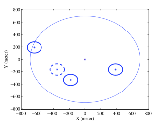
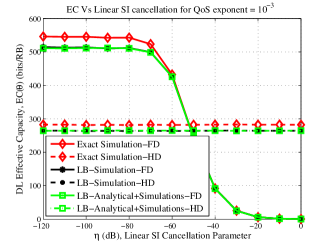
Figure 3: A specific instance of sparse small cell deployment as obtained using a Hard Core Matérn PP with density $\lambda=5\,\textrm{small cell/km}$² (a), and corresponding DL effective capacity experienced by a typical UE (uniformly distributed in the dashed small–cell) vs. linear self–interference suppression ratio, for HD and FD (exact and lower bounds) (b). QoS exponent $\theta=10^{-3}$ (1/bit), non linear self–interference cancellation parameter $\kappa=1$.

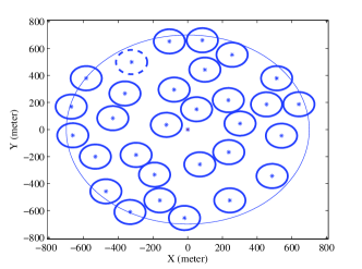
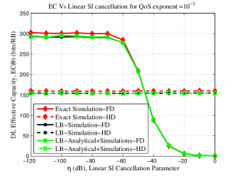
Figure 4: A specific instance of dense small cell deployment as obtained using a Hard Core Matérn PP with density $\lambda=50\,\textrm{small cell/km}$² (a), and corresponding DL effective capacity experienced by a typical UE (uniformly distributed in the dashed small–cell) vs. linear self–interference suppression ratio, for HD and FD (exact and lower bounds) (b). QoS exponent $\theta=10^{-3}(1/bit)$, non linear self–interference cancellation parameter $\kappa=1$.

Fig. 3 refers to a sparse system, with $\lambda=5$ small cells per km², and reports the downlink (DL) effective capacity versus the linear SI cancellation parameter, for QoS exponent $\theta=10^{-3}$. For the given QoS exponent, it can be inferred that a maximum gain of 1.93X can be achieved with the help of a perfect FD system. A similar maximum gain of 1.89X is reported in Fig. 4, this time for the realization of a denser Matérn HCPP with $\lambda=50$ small cells per km² and a QoS exponent $\theta=10^{-3}$. In both cases, a trade–off value for the linear SI cancellation parameter at which the FD operation mode outperforms HD in terms of downlink EC can be found, namely $-50$ dB for the former scenario and $-45$ dB for the latter. Moreover, most of the maximum FD gain obtainable can already be achieved for $\eta=-80$ dB in the first scenario and $\eta=-70$ dB for the second one, which are readily provided by current technology. In both scenarios, the non linear SI cancellation parameter was set to $\kappa=1$.

The second important result that can be observed from these figures is the fact that the lower bound proposed in (13) is tight. Specifically, the black curves, for the lower bound computed through simulations, and the green ones, for the lower bound computed through analysis and simulations, are practically overlapped and very close to the red curves that report the exact value of EC.

It is worth observing that the lower bound is closer to the exact values if the system becomes more crowded, i.e., for a higher density of BSs. In addition, as tabulated in Table II and discussed in Section IV, the analytical approach has a complexity almost independent of the network size and significantly lower with respect to the exact computation of EC. Thus, our method to analyze statistical QoS performance of HCN is scalable with the network size.

TABLE II: Time Elapsed in Analyzing the System Performance

Scenario	Exact Analysis	Proposed Lower Bound
Fig. 3	370 s	17 s
Fig. 4	2220 s	21 s

VI Conclusions

In this paper we introduced a lower bound for the evaluation of the effective capacity in a generic wireless scenario. Based on the proposed lower bound we built a scalable mathematical framework to analyze the statistical QoS performance of dense next generation HCNs. Our proposed scheme helped us analyze HD and imperfect FD HCNs from an EC perspective with very good accuracy at only a fraction of the complexity needed for an exact analysis.

References

- [1] Ericsson Press Release, “Ericsson mobility report,” February 2015.
- [2] J. Andrews, S. Buzzi, W. Choi, S. Hanly, A. Lozano, A. Soong, and J. Zhang, “What will 5G be?” IEEE Journal on Selected Areas in Communications, vol. 32, no. 6, pp. 1065–1082, June 2014.
- [3] A. Ghosh, N. Mangalvedhe, R. Ratasuk, B. Mondal, M. Cudak, E. Visotsky, T. Thomas, J. Andrews, P. Xia, H. Jo, H. Dhillon, and T. Novlan, “Heterogeneous cellular networks: From theory to practice,” IEEE Communications Magazine, vol. 50, no. 6, pp. 54–64, June 2012.
- [4] A. Sabharwal, P. Schniter, D. Guo, D. Bliss, S. Rangarajan, and R. Wichman, “In-band full-duplex wireless: Challenges and opportunities,” IEEE Journal on Selected Areas in Communications, vol. 32, no. 9, pp. 1637–1652, Sept 2014.
- [5] D. Bharadia, E. McMilin, and S. Katti, “Full duplex radios,” in ACM SIGCOMM Computer Communication Review, vol. 43, no. 4, 2013, pp. 375–386.
- [6] M. Duarte, C. Dick, and A. Sabharwal, “Experiment-driven characterization of full-duplex wireless systems,” IEEE Transactions on Wireless Communications, vol. 11, no. 12, pp. 4296–4307, December 2012.
- [7] X. Zhang, W. Cheng, and H. Zhang, “Heterogeneous statistical QoS provisioning over 5G mobile wireless networks,” IEEE Network, vol. 28, no. 6, pp. 46–53, Nov 2014.
- [8] D. Wu and R. Negi, “Effective capacity: a wireless link model for support of quality of service,” IEEE Transactions on Wireless Communications, vol. 2, no. 4, pp. 630–643, July 2003.
- [9] D. Ramirez and B. Aazhang, “Optimal routing and power allocation for wireless networks with imperfect full-duplex nodes,” IEEE Transactions on Wireless Communications, vol. 12, no. 9, pp. 4692–4704, September 2013.
- [10] X. Zhang, J. Tang, H.-H. Chen, S. Ci, and M. Guizani, “Cross-layer-based modeling for quality of service guarantees in mobile wireless networks,” IEEE Communications Magazine, vol. 44, no. 1, pp. 100–106, January 2006.
- [11] H. ElSawy, E. Hossain, and M. Haenggi, “Stochastic geometry for modeling, analysis, and design of multi-tier and cognitive cellular wireless networks: A survey,” IEEE Communications Surveys Tutorials, vol. 15, no. 3, pp. 996–1019, March 2013.
- [12] H. Dhillon, R. Ganti, F. Baccelli, and J. Andrews, “Modeling and analysis of K-tier downlink heterogeneous cellular networks,” IEEE Journal on Selected Areas in Communications, vol. 30, no. 3, pp. 550–560, April 2012.
- [13] J. Andrews, F. Baccelli, and R. Ganti, “A tractable approach to coverage and rate in cellular networks,” IEEE Transactions on Communications, vol. 59, no. 11, pp. 3122–3134, November 2011.
- [14] E. Dahlman, S. Parkvall, and J. Skold, 4G: LTE/LTE-advanced for mobile broadband. Academic press, 2013.