Josephson effects in an alternating current biased transition edge sensor

Abstract

We report the experimental evidence of the ac Josephson effect in a transition edge sensor (TES) operating in a frequency domain multiplexer and biased by ac voltage at MHz frequencies. The effect is observed by measuring the non-linear impedance of the sensor. The TES is treated as a weakly-linked superconducting system and within the resistively shunted junction model framework. We provide a full theoretical explanation of the results by finding the analytic solution of the non-inertial Langevian equation of the system and calculating the non-linear response of the detector to a large ac bias current in the presence of noise.

Superconducting transition-edge sensors (TESs) are highly sensitive thermometers widely used as radiation detectors over an energy range from near infrared to gamma rays. In particular we are developing TES-based detectors for the infrared SAFARI/SPICARoelfsema et al. (2014) and the X-ray XIFU/AthenaRavera et al. (2014) instruments. TESs are in most cases low impedance devices that operate in the voltage bias regime while the current is generally read-out by a SQUID current amplifier. Both a constant or an alternating bias voltage can be used Irwin and Hilton (2005); van der Kuur et al. (2002). In the latter case changes of the TES resistance induced by the thermal signal modulate the amplitude of the ac bias current. The small signal detector response is modelled in great details both under dc and ac bias Swetz et al. (2012); van der Kuur et al. (2011). Those models however do not fully explain all the physical phenomena recently observed in TESs. It has been recently demonstrated that TES-based devices behave as weak-links due to longitudinally induced superconductivity from the leads via the proximity effect Sadleir et al. (2010) and a detailed experimental investigation of the weak-link effects in dc biased x-ray microcalorimeters has been reported Smith et al. (2013). Evidence of weak-link effects in ac biased TES microcalorimeters has been given Gottardi et al. (2012), but an adequate experimental and theoretical investigation is still missing. We previously proposed a theoretical framework Kozorezov et al. (2011) based on the resistively shunted junction model (RSJ) that can be used to describe the resistive state of a TES under dc bias. In this letter, we extend the model to calculate the stationary non-linear response of a TES to a large ac bias current in the presence of noise and we compare it to the experimental data obtained with a TES-based bolometer. We report a clear signature of the ac-Josephson effect in the TES biased at MHz frequencies.

The general equation for the Frequency Domain Multiplexing (FDM) electrical circuit, simplified for a single resonator isvan der Kuur et al. (2011)

$$V(t)=I(t)Z_{TES}(T,I(t))+L\frac{dI(t)}{dt}+\frac{1}{C}\int I(t)dt+r_{s}I(t)$$ (1)

where $V(t)$ is the total voltage across the TES, $L$ and $C$ are respectively the inductance and the capacitance of the bias circuit, $r_{s}$ is the total stray resistance in the circuit and $Z_{TES}$ is the TES impedance, which depends on temperature $T$ and current $I(t)$. As previously reported Sadleir et al. (2011); Smith et al. (2013), the superconducting leads proximitize the TES bilayer film over a distance defined by the coherence length $\xi$. As a result, the superconducting order parameter $|\Psi|$ is spatially dependent over the length of the bilayer, as shown in the cross section of Fig. (1)(b) . The TES can be seen then as an $SS^{\prime}S$ proximity induced weak-link where the electrical bias leads and the Ti/Au bilayer are the $S$ and $S^{\prime}$ materials respectively.

The electrical scheme of the ac bias read-out and the TES representation as a weak-link are shown in Fig. (1). We describe the TES using the RSJ model in which the resistance is replaced by an ideal junction shunted by the TES normal resistance $R_{N}$ Likharev (1979); Kozorezov et al. (2011).

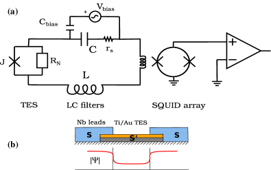
Figure 1: (a) Electrical circuit of the ac-bias read-out where the TES is modelled as a resistively shunted junction. (b) Cross section of the TES bilayer with Nb leads and the dependence on the superconducting order parameter over the TES length.

Within this model, the total current $I(t)$ flowing between two weakly connected superconductors can be described by the two Josephson equations as

$$I(t)+\mathcal{L}(t)=I_{c}\sin\varphi+\frac{V(t)}{R_{N}},\;\;\;\frac{\partial\varphi}{\partial t}=\frac{2e}{\hbar}V(t)$$ (2)

where $\varphi$ is the gauge-invariant phase difference between the wave functions of the two superconductors and $I_{c}$ is the critical current. $\mathcal{L}(t)$ is a thermal fluctuation noise current superimposed on the bias current generated by the fact that the weak-link operates at temperature $T$ above absolute zero Ambegaokar and Halperin (1969); Coffey, Dejardin, and Kalmykov (2000). $\mathcal{L}(t)$ is assumed to be Gaussian white noise with $\overline{\mathcal{L}(t)}=0$ and $\overline{\mathcal{L}(t)\mathcal{L}(t^{\prime})}=\frac{2kT}{R_{N}}\delta(t-t^{\prime})$.

It follows from the second of the Josephson Eqs. (2) that in a TES under ac bias voltage $V(t)=V_{ac}\cos\omega_{0}t$ the superconducting phase $\varphi$ oscillates at the same bias frequency $\omega_{o}$, but $\pi/2$-out-of-phase with respect to the voltage. The total current flowing in the TES is then a superposition of a supercurrent and a normal current caused by the flow of quasiparticle across the junction.

Within this context we evaluate the stationary nonlinear response of a TES for a large ac bias current and in the presence of noise. For a given ac bias current $I(t)=I_{ac}\cos\omega_{0}t$, from Eqs. (2), we can derive $\varphi$ by solving the non-inertial Langevin equation for the RSJ model with noise:

$$\frac{\tau}{\gamma}\frac{\partial\varphi}{\partial t}+\sin\varphi=\zeta\cos\omega_{0}t+I_{c}^{-1}\mathcal{L}(t),$$ (3)

where $\tau=\left(\hbar/2e\right)^{2}/R_{N}k_{B}T$ is the averaged time a particle takes to diffuse one period of a tilted washing board potential, $\zeta=I_{ac}/I_{c}$ and $\gamma=\hbar I_{c}/\left(2ek_{B}T\right)$ is the normalised Josephson coupling energy, a parameter which also characterises the noise strength with $\gamma=\infty$ corresponding to the noiseless limit. The total phase difference across the weak-link $\varphi$ depends as well on the external magnetic flux coupled into the TES and its expression can be generalised as $\varphi_{tot}=\varphi+2\pi\frac{\Phi(t)}{\Phi_{0}}$. In the first approximation $\Phi(t)=A_{eff}(B_{\perp,DC}+B_{\perp,AC}(t))$ where $A_{eff}$ is the effective weak-link area and $B_{\perp,DC}$ and $B_{\perp,AC}(t)$ the dc and ac perpendicular magnetic field crossing the TES respectively.

The solution of Eq. (3) for the stationary state can be found analytically in terms of matrix continued fraction Coffey, Dejardin, and Kalmykov (2000). The non-linear admittance of the weakly superconductive TES at the carrier frequency $f_{0}=\omega_{0}/2\pi$ can be derived in the form

$$\frac{1}{Z_{TES}}=\frac{1}{R_{TES}}-j\frac{1}{\omega_{0}L_{J}}=\frac{1}{R_{N}\left(1-j\zeta\left[c^{1}_{1}(\omega)-c^{1*}_{1}(-\omega)\right]\right)},$$ (4)

with the non-linear Josephson inductance $L_{J}$ in parallel with the TES resistance $R_{TES}$.

The elements of the vector ${\bf c_{n}}$ can be calculated from the following equations

$$\begin{array}[]{lll}{\bf c}_{n}&=&{\bf S}_{n}^{21}{\bf c}_{0},\\ \\ {\bf S}^{21}_{n}&=&({\bf q}_{2n-1}+({\bf q}_{2n}+{\bf S}^{21}_{n+1})^{-1})^{-1},\end{array}$$ (5)

where the tridiagonal infinite matrices ${\bf q_{n}}$ can be written as

$$\begin{array}[]{lll}{\bf q}_{n}&=&j\left(\begin{matrix}\ddots&\vdots&\vdots&\vdots&\vdots&\vdots&\iddots\\ \ldots&z_{n}^{-2}&\zeta&0&0&0&\ldots\\ \ldots&\zeta&z_{n}^{-1}&\zeta&0&0&\ldots\\ \ldots&0&\zeta&z_{n}^{0}&\zeta&0&\ldots\\ \ldots&0&0&\zeta&z_{n}^{1}&\zeta&\ldots\\ \ldots&0&0&0&\zeta&z_{n}^{2}&\ldots\\ \iddots&\vdots&\vdots&\vdots&\vdots&\vdots&\ddots\end{matrix}\right)\end{array}$$ (6)

and the vector ${\bf c}_{0}=\left(\ldots\;0\;1\;0\;\ldots\right)^{T}$. The diagonal elements in Eq. (6) are defined as

$$z_{n}^{m}(\omega)=2\left(m\omega\tau/\left(n\gamma\right)-jn/\gamma\right),$$ (7)

with $m=\{\ldots,-1,0,1,\ldots\}$ and $n=\{1,2,\ldots\}.$

We assume the TES to be ac biased with the bias current derived from the temperature and current dependent resistance $R_{TES}(T,I)$ and the effective power balance equation.

The FDM read-out of TESs measures naturally the resistive $R_{TES}$ and reactive $X=\omega_{o}L_{J}$ components of the TES non-linear impedance in Eq. (4) by performing the in-phase and quadrature detection of the TES current. By measuring both the amplitude $I_{ac}$ and the phase $\theta$ of the TES current with respect to the applied voltage $V_{ac}$ we obtain the TES non-linear impedance $Z_{TES}=V_{ac}/I_{ac}e^{-j\theta}$. The effective power of a TES with resistance $R_{TES}(T,I)$ under ac bias is given byvan der Kuur et al. (2011)

$$\frac{V_{ac}I_{ac}}{2}\cos\theta=\frac{1}{2}I_{ac}^{2}R_{TES}(T,I)\cos^{2}\theta=k(T^{n}-T^{n}_{b}),$$ (8)

where $k=G/n(T^{n-1})$ with $G$ the differential thermal conductance, $n$ is the thermal conductance exponent and $T_{b}$ is the bath temperatureIrwin and Hilton (2005).

The vectors ${\bf c}_{n}$ can be calculated numerically by computing the matrix continued fraction in Eq. (5) and solving simultaneously the power balance equation Eq. (8). The convergence is rapidly achieved for the parameters discussed below.

The set-up used for the experiments presented in this paper is an FDM system working in the frequency range from 1 to 5 MHz, based on an open-loop or baseband feedback read-out of a linearised two-stage SQUID amplifier and high$-Q$ lithographic $LC$ resonators Gottardi et al. (2014). Here below we report the results for a TES ac biased at frequencies of $1.4\,\text{and}\,2.4\,\mathrm{MHz}$. The device under test is a bolometer based on a square Ti/Au (16/60 nm) bilayer TES $L\times L=50\times 50\,\mu\mathrm{m^{2}}$ in size. It has a critical temperature at zero magnetic field of $T_{c}=85.5\,\mathrm{mK}$, a normal state resistance of $R_{N,tes}=98\,\mathrm{m\Omega}$, a thermal conductance to the bath $G=0.3\,\mathrm{pW/K}$ and a measured NEP under ac bias of $3.5\times 10^{-19}\,\mathrm{W/\sqrt{Hz}}$ Gottardi et al. (2014). The electrical contact to the bolometer is realised by $90\,\mathrm{nm}$ thick Nb leads deposited on the edges of the bilayer as shown in Fig. (1). We report strong evidence of proximity induced weak-link behaviour of our TES-based bolometer measured under ac bias. The three main experimental observations are: the modulation of the TES critical current $I_{c}$ under applied magnetic field $B$, showing the typical Fraunhofer-like pattern of a Josephson junction; the exponential dependence on the critical current on temperature $T$ and the presence of a non-linear reactance modulated by the TES bias voltage.

The measured critical current $I_{c}(T,B)$ is shown in Fig. (2) as a function of temperature $T$ and the applied perpendicular dc magnetic field $B_{\perp,DC}$.

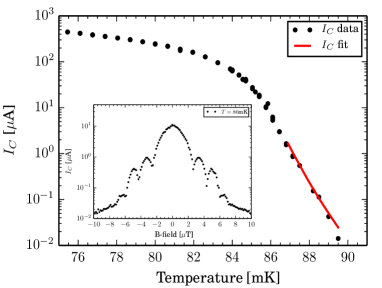
Figure 2: TES critical current as a function of the bath temperature at zero magnetic field and (inset) as a function of the applied perpendicular magnetic field at $T=86\,\mathrm{mK}$. The TES is ac biased at a frequency of $2.4\,\mathrm{MHz}$. The model Sadleir et al. (2010); Likharev (1979) fit the data in the TES $R(T,I)$ sharp transition range (red line).

For $T\geq T_{c}$ the critical current of the TES shows an exponential dependence on $T$ and can be fitted (see red line in Fig. (2)) by the approximated formula $I_{c}(L,T)\propto e^{-\frac{L_{wl}}{\xi_{0}}|\frac{T}{T_{Ci}}-1|^{1/2}}$ to estimate the Josephson contribution to $I_{c}$ from the weak-link model Sadleir et al. (2010); Likharev (1979). Here $L_{wl}\leq L$ is the effective size of the TES along the current flow operating as a weak-link, $\xi_{0}$ is the zero temperature coherence length and $T_{Ci}$ is the intrinsic critical temperature of the laterally unproximised TiAu bilayer.

The periodicity of the oscillations in the Fraunhofer pattern of $I_{c}(B)$ is defined as $\Delta B_{min}=\Phi_{0}/LL_{wl}$ where $\Delta B_{min}$ is the magnetic field difference between the local minima in $I_{c}(B)$. From the data we inferred that only a fraction $f=\frac{\Delta B_{min}L^{2}}{\Phi_{0}}=\frac{L_{wl}}{L}=0.67$ of the geometrical TES area $L^{2}$ behaves as a weak-link. The explanation for this experimental result requires a detailed study of the electrodynamics of long junctions and goes beyond the scope of this paper. The fact that the magnetic field penetrates only part of the TES has implication for the choice of the value of the normal resistance used in the RSJ model presented below.

The TES resistive state is calculated by simulating the resistive transition within the RSJ model for dc-biased TES Kozorezov et al. (2011) and using as input parameters the experimental critical current curve $I_{c}(T)$ and the TES normal resistance. The use of the functional dependence $R(T,I)$ calculated for the dc bias case is justified by the our previous results Gottardi et al. (2014) where we have shown that the IV curves measured under ac and dc bias are identical within the experimental errors. Because only $67\%$ of the TES area is proximized we assume the normal resistance of the weak-link to be $R_{N}=0.67R_{N,tes}$.

The use of the general formalism of continued fraction matrices to solve Eq. (3) requires self-consistent numerical solution of the balance equation Eq. (8). We developed the code which allows to implement this procedure and calculate the in-phase and quadrature components of the TES current and the non-linear impedance of the weakly superconducting TES as given in Eq. (4). The experimental in-phase and quadrature TES current components are plotted in Fig. (3) versus the TES bias voltage for $1.4$ and $2.4\,\mathrm{MHz}$ bias frequencies. The curves calculated using the RSJ model are also shown.

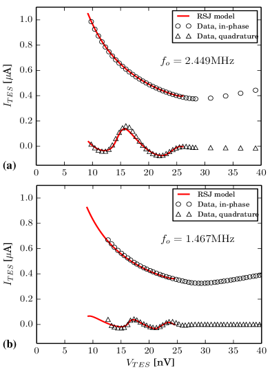
Figure 3: TES $I-V$ characteristics showing both the in-phase (open circle) and quadrature (open triangle) components of the current. The measurements where taken at a bias frequency of 2.4 (a) and $1.4\,\mathrm{MHz}$ (b) and at a bath temperature of $30$ and $40\,\mathrm{mK}$ respectively. The solid lines are the $IV$ curves obtained from the RSJ model.

The IV curve obtained using the in-phase component of the TES current is consistent with the results obtained with the same pixel measured under dc-bias Gottardi et al. (2014). The quadrature component of the current shows an oscillatory behaviour dependent on the driving bias frequency. Generally, the period and the amplitude of the oscillations decreases with the bias frequency. Moreover, the amplitude is larger at low bias voltages due to the fact that the noise parameter $\gamma$ increases when the TES is biased low in the transition. Both observations are consistent with the numerical calculation performed by Coffey et al.Coffey, Dejardin, and Kalmykov (2000) on Josephson junctions. For the detector under test the $\pi/2$-out-phase current reaches a maximum peak amplitude of about $10\%$ and $20\%$ of the total current flowing in the TES for a driving frequency of $1.4\,\mathrm{MHz}$ and $2.4\,\mathrm{MHz}$ respectively.

The measured and calculated TES resistance $R_{TES}$ and Josephson inductance $L_{J}$ as a function of the bias voltage and temperature are shown respectively in Fig. (4) and Fig. (5) for the detector that was biased at $f_{o}=2.4\,\mathrm{MHz}$.

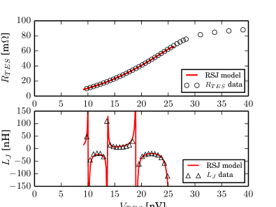
Figure 4: The TES resistance $R_{TES}$ (open circle) and the Josephson inductance $L_{J}$ (open triangle) as a function of the voltage bias. The TES is ac biased at a frequency of 2.4 MHz. The solid lines show the results from the RSJ model.

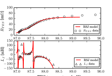
Figure 5: TES resistance $R_{TES}$ (open circle) and Josephson inductance $L_{J}$ (open triangle) as a function of temperature $T$ derived from the $I-V$ curves and the power balance equation. The TES is ac biased at a frequency of 2.4 MHz. The solid lines show the result from the RSJ model.

The TES behaves as a nonlinear inductor in parallel with a resistance as predicted by the RSJ model. The nonlinear inductance oscillates between positive and negative values in the superconducting transition. At some particular bias voltage the inductance becomes infinite and the TES is purely resistive.

The $R(T)$ curves of the TES for $T>T_{c}$ show typically a sharp resistive transition above which the resistance is not constant, but has a small nonzero slope. The RSJ model explains the shape of the sharp transition, while, as shown by Sadleir et al.Sadleir et al. (2011) the enhanced conductivity above the sharp phase transition can be well fitted under the assumption that zero-resistance region penetrates a distance twice the temperature dependent coherence length of the infinite bi-layer from both leads.

In conclusion, we observed a clear signature of the ac Josephson effect in a TES bolometer operating under ac bias at frequencies of few MHz. The effect clearly appears in the quadrature component of the bias current. We applied the RSJ model and calculated the stationary non-linear response of a TES under ac bias and in the presence of noise. Using the analytic expressions for the non-linear admittance of a weakly superconducting TES changing in accordance with the power balance variation through the resistive transition we can fully reproduce the measured TES resistance and the Josephson inductance as a function of bias voltage, bias frequency and operating temperature.