Isogeometric analysis for functionally graded microplates based on modified couple stress theory

Abstract

Analysis of static bending, free vibration and buckling behaviours of functionally graded microplates is investigated in this study. The main idea is to use the isogeometric analysis in associated with novel four-variable refined plate theory and quasi-3D theory. More importantly, the modified couple stress theory with only one material length scale parameter is employed to effectively capture the size-dependent effects within the microplates. Meanwhile, the quasi-3D theory which is constructed from a novel seventh-order shear deformation refined plate theory with four unknowns is able to consider both shear deformations and thickness stretching effect without requiring shear correction factors. The NURBS-based isogeometric analysis is integrated to exactly describe the geometry and approximately calculate the unknown fields with higher-order derivative and continuity requirements. The convergence and verification show the validity and efficiency of this proposed computational approach in comparison with those existing in the literature. It is further applied to study the static bending, free vibration and buckling responses of rectangular and circular functionally graded microplates with various types of boundary conditions. A number of investigations are also conducted to illustrate the effects of the material length scale, material index, and length-to-thickness ratios on the responses of the microplates.

1 Introduction

Functionally graded materials (FGMs), which are initially proposed by group of Japanese aerospace researchers, are composite materials formed of two or more constituent phases in which material properties vary smoothly from one surface to the other. Consequently, FGMs are able to avoid high interlaminar shear stresses, stress concentration and delamination phenomenon which are often cited as shortcomings of laminated composite materials. A FGM consisting of ceramic and metal possesses higher thermal resistance and better ductility which are inherited from the ceramic and metal phases, respectively. Owning these striking features, FGMs are applicable to various fields of engineering including aerospace, nuclear power, chemistry and biology engineering. The FGMs are also widely studied within various types of structure such as beams [1, 2, 3, 4], plates [5, 6, 7, 8], and shells [9, 10, 11].

Recent advances in technology lead to new industrial fields in which small-scale elements are involved. Such elements have been applied in the micro- and nano-electro-mechanical system [12, 13], actuators [14], space and bio-engineering [15]. These applications encourage new research area that focuses on investigating and predicting the behaviours of such micro structures. A number of attempts have been conducted to analyse characteristic of small-scale structures including experiment and computer simulation [16, 17]. Nevertheless, while the former is mechanical and economical challenging due to the extremely small size of the elements, the latter exponentially raises computational cost. Therefore, the mathematical and mechanical models which account for the small-scale effects are needed. It is widely known that the behaviour of small-scale structures is size-dependent. This is confirmed following a number of theoretical and experimental works of Fleck et al. [18], Stolken and Evans [19], and Lam et al. [20]. Having an experimental observation from bending test of epoxy polymeric microbeams, Lam et al. [20] point out that the bending rigidity increases $2.4$ times as a result of the reduction of beam thickness from $115$ $\mu$m to $20$ $\mu$m.

In order to take into account the size effects, based on the classical elasticity theories, a number theories have been developed including nonlocal elasticity theory [21], strain gradient theory [22], and modified couple stress theory [23]. It is worth noting that the classical elasticity is fundamentally founded by the introduction of the Hook’s Law in which the force and the change in displacement are linearly related via the stiffness of the component where the forces are applied. This principal of physics governs the linearly elastic behaviours of materials. As physics and mechanics develop, stress and strain which are linearly connected via the elastic modulus are cited as the primary measures of classical elasticity rather than force and displacement counterparts. Aiming for better prediction of materials’ responses, Mindlin and Tiersten [24] and Mindlin [25] have initially developed higher-order theories of elasticity. Based on the employment of deformation metrics, those theories could be classified into two categories including strain gradient and couple stress theories. With regard to the strain gradient theories, this concept was first developed by Fleck and Hutchinson [22] in which the Mindlin’s theory [25] was extended. There are two components, which are classified using the second-order deformation tensor that include stretch gradient tensor and rotation gradient tensor [26]. Within the concept of couple stress theory, both strain and curvature jointly govern the strength of the solid. In addition, while the antisymmetric part of the second-order deformation gradients is served as rotation gradients, the symmetric part is neglected. Based on the initial ideas of couple stress theory, a number of attempts have been conducted to further develop the concepts that are applicable for size-dependent problems. Yang et al. [23] proposed the equilibrium of moment of couples which was an additional equilibrium relation that forces the couple stress tensor to be symmetric. Therefore, the deformation energy is only influenced by the symmetric part of rotation gradient and the symmetric part of displacement gradient. In addition, instead of using two material length scale parameters as need in the classical couple stress theory, this modified couple stress theory (MCST) requires only one material length scale parameter to construct the constitutive relation. Park and Gao [27] utilised the principle of minimum total potential energy to develop a variational formulation of the modified couple stress theory. This method not only derives the equilibrium equations but also forms the determination of boundary conditions which are not available in the Yang’s theory [23]. In recent years, the modified couple stress theory has been applied to study the various behaviours of small-scale structures. For beam analysis, static bending, buckling, and vibration analysis have been conducted using Euler-Bernoulli [28], Timoshenko [29, 30, 31, 32], and higher-order beam theories [33]. The modified couple stress theory was also applied in the small-scale plate analysis in several ways, Tsiatas [34] initially employed MCST to investigate the static bending response of isotropic Kirchhoff microplates. Yin et al. [35] solely investigated the vibration behaviour of Kirchhoff microplates using the standard separation of variables to derive the closed-form solution for natural frequency. Bending and vibration behaviours of Mindlin microplates were studied by Ma et al. [36] in which the thickness stretching effect was also taken into account. With regard to the small-scale functionally graded (FG) structures, a number of investigations have been conducted for micro FG beams and plates. Simsek et al. [37] investigated the static bending of functionally graded microbeams based on the modified couple stress theory. Buckling behaviour of FG microbeams was studied by Nateghi et al. [38]. Based on the modified couple stress theory, Reddy et al. [39, 40, 41, 42] studied nonlinear behaviour of small-scale FG microplates with different geometry shapes. Thai and his colleagues utilised the Navier’s approach to derive solutions for FG microplates in which Kirchoff, Minlind and sinusoidal plate theories were used along with the MCST [43, 44, 45]. Ke et al. [46, 47] employed $p$-version Ritz method and different quadrature method to solve free vibration and bending, buckling problems of the rectangular and annular FG Mindlin microplates based on MCST, respectively. Using modified couple stress theory, a refined plate theory was utilised to predict the bending, buckling, and vibration behaviours of FG microplates by He et al. [48] following the Navier’s approach. Most of these efforts followed analytical approach which was able to solve some specific types of boundary condition.

A large proportion of the studies in small-scale FG structures employ the classical plate theory (CPT) and the first-order shear deformation theory (FSDT). However, the classical plate theory (or the Kirchoff-Love theory), which neglects shear deformation, provides acceptable solutions for thin plates, i.e. length-to-thickness ratios are quite large, only. Meanwhile, the first-order shear deformation theory (or Reissner-Mindlin plate theory), which accounts for transverse shear effects, is applicable for both thin and moderately thick plates [49, 50, 51]. The shortcomings of the FSDT include inaccurate distribution of transverse shear strain/stress and violation of traction free boundary conditions at top and bottom surfaces. For this reason, shear correction factors are required to adjust the transverse shear stress distribution. However, these factors vary from problems and one may find it difficult to choose an appropriate value. In order to avoid using shear correction factors, the third-order shear deformation theory (TSDT) [52], higher-order shear deformation theory (HSDT) [53], sinusoidal shear deformation theory (SSDT) [54], and refined plate theories (RPT) [55] have been developed yielding more accurate and reliable results. The refined plate theory is initially proposed by Senthilnathan et al. [55] by employing four unknowns and is one variable less than that of TSDT. Shimpi et al. [56, 57, 58] then further developed the RPT for isotropic and orthotropic plates by using only two variables. However, HSDT and RPT require C¹-continuity of general displacements which cause significant challenge to derive second derivative of deflection in the platform of finite element analysis (FEA) where C⁰ elements are frequently used. In order to overcome the continuity issues, some C⁰ approximations [59] and Hermite interpolation functions with C¹ elements [8] which involve adding extra unknown variables of derivative of displacement are adopted.

Recently, a new numerical method so-called Isogeometric Analysis (IGA) which is able to deal with C¹-continuity problem without using any additional variables or Hermite interpolation function has been introduced by Hughes and his co-workers [60]. This method bridges the existing gap between the fields of finite element analysis and computer-aided design (CAD). The essential idea of the isogeometric analysis is that the basis functions which are employed to exactly describe the geometry domain will also be used for approximations of unknown fields. Since geometry is exactly modeled and the number of unknown terms is not increased, it is expected that IGA would yield more accurate results with lower computational cost for HSDT and RPT problems in the comparison with regular FEA [61]. One may find the guidance on computer implementation of IGA in the open literature [62, 63, 64]. IGA has been widely implemented in a number of linearly and non-linearly mechanical and thermal problems such as static, free vibration, and buckling of laminated composite and functionally graded plates with various plate theories including layerwise, FSDT, HSDT, and RPT [65, 66, 67, 53, 68, 61, 69, 70, 71, 72, 73]. However, as far as author’s knowledge, there is no publication dealing with analysis of small-scale plates based on modified couple stress theory and NURBS basis functions.

In this study, in order to fill the aforementioned gap, the bending, free vibration and buckling behaviours of FG microplates based on the modified couple stress theory and four-variable refined plate and quasi-3D theories is investigated in conjunction with the isogeometric approach. While the modified couple stress theory is employed to capture the small-scale effects, the displacement fields of those microplates are expressed based on a novel seventh-order RPT and quasi-3D theory. The mechanical behaviours of FG microplates are then solved by the isogeometric analysis in which NURBS functions are simultaneously used to exactly describe the geometry boundaries and construct the basis functions of the approximations.

The outline of this study is expressed as follow. The next section presents theories which are applicable for analysis of FG microplates including modified couple stress theory, RPT and quasi-3D theory. In addition, a brief note on functionally graded material will also be introduced in this section. Section 3 focuses on the isogeometric and NURBS-based formulation of quasi-3D theory. The numerical examples which cover static bending, free vibration and buckling analysis of rectangular and circular FG microplates with various boundary conditions will be provided in Section 4. Finally, some conclusions will be drawn in Section 5.

2 A novel theory for FG microplates

In this section, a brief review on the formulation of modified couple stress theory with only one material length scale that accounts for size-dependent effects is firstly presented. It is followed by the theoretical definition of functionally graded material of which microplates are made. Displacement field of plates is then derived based on the four-variables refined plate theory and quasi-3D plate theory where a novel seventh-order shear deformation theory is proposed.

2.1 Modified couple stress theory

According to the modified couple stress theory which is proposed by Yang et al. [23], the strain energy density $w$ for linear isotropic material is a quadratic function of generalized strains

$$w=\frac{1}{2}\lambda\left({\text{tr}{\boldsymbol{{\bf{\varepsilon}}}}}\right)^{2}+\mu\left({{\boldsymbol{{\bf{\varepsilon}}}}:{\boldsymbol{{\bf{\varepsilon}}}}+l^{2}{\boldsymbol{\chi}}:{\boldsymbol{\chi}}}\right),$$ (1)

where $\lambda$ and $\mu$ are Lame’s constants, $\mu$ is also known as shear modulus which is often denoted as $G$, $l$ represents material length scale parameter and the strain tensor $\boldsymbol{{\bf{\varepsilon}}}$ and symmetric curvature tensor $\boldsymbol{\chi}$ are defined by

$${\boldsymbol{{\bf{\varepsilon}}}} =\frac{1}{2}\left[{\nabla{\bf{u}}+\left({\nabla{\bf{u}}}\right)^{T}}\right],$$ (2a)

$${\boldsymbol{\chi}} =\frac{1}{2}\left[{\nabla{\boldsymbol{\theta}}+\left({\nabla{\boldsymbol{\theta}}}\right)^{T}}\right],$$ (2b)

where $\bf{u}$ is displacement vector and the rotation vector $\boldsymbol{\theta}$ is given by

$${\boldsymbol{\theta}}=\frac{1}{2}\text{curl}\left({\bf{u}}\right).$$ (3)

The strain energy $U$ restored in a deformed elastic body is then defined as

$$U=\int\limits_{V}{wdV}=\int\limits_{V}{\left({{\boldsymbol{\sigma}}:{\boldsymbol{{\bf{\varepsilon}}}}+{\bf{m}}:{\boldsymbol{\chi}}}\right)dV},$$ (4)

where $\boldsymbol{\sigma}$ and $\bf{m}$ are the symmetric stress tensor and the deviatoric part of the couple stress tensor, respectively. These components, $\boldsymbol{\sigma}$ and $\bf{m}$, which are conjugated to the deformation measures $\boldsymbol{{\bf{\varepsilon}}}$ and $\boldsymbol{\chi}$, respectively, are given as

$${\boldsymbol{\sigma}} =\lambda\left({\text{tr}{\boldsymbol{{\bf{\varepsilon}}}}}\right){\bf{I}}+2\mu{\boldsymbol{{\bf{\varepsilon}}}},$$ (5a)

$${\bf{m}} =2\mu l^{2}{\boldsymbol{\chi}},$$ (5b)

where $\bf{I}$ is the identity matrix. Apparently, Eq. (5) shows there is only one material length scale needed and the deviatoric couple stress tensor $\bf{m}$ is also symmetric, from which the modified couple stress theory is formed.

2.2 Functionally graded material

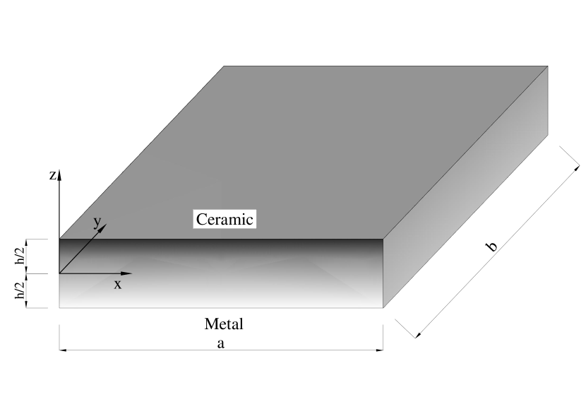
Figure 1: The functionally graded microplate model.

The model configuration of the functional graded material which is made of metal and ceramic is illustrated in Figure 1. There are several homogeneous models that are employed to estimate the effective properties of the FGMs. According to the rule of mixtures, the corresponding effective properties of the FGMs could be expressed as follow

$$P_{e}=P_{m}V_{m}+P_{c}V_{c},$$ (6)

where $P_{m}$ and $P_{c}$ are the material properties of metal and ceramic phases, respectively, including Young’s modulus $E$, density $\rho$ and Poisson’s ratio $\nu$. Meanwhile, $V_{m}$ and $V_{c}$ represent the volume fraction of metal and ceramic phases, respectively, which could be defined as follow [8]

$$V_{c}\left(z\right)=\left({\frac{1}{2}+\frac{z}{h}}\right)^{n},\quad V_{m}=1-V_{c},\quad-\dfrac{h}{2}\leq z\leq\dfrac{h}{2},$$ (7)

where $n$ is the material index. This equation implies smooth variation in material properties of FGM is guaranteed and governed by the material index $n$. As can be inferred from Eq. (7), $n=0$ leads to a FGM with fully homogeneous ceramic while the FGM becomes fully metal as $n$ goes toward $\infty$. Nevertheless, the rule of mixtures model fails to describe the interaction between the material phases [74, 75]. Therefore, Mori-Tanaka scheme [76, 77] is developed to fill this gap in estimation of FGM’s properties by integrating effective bulk modulus $K_{e}$ and shear modulus $G_{e}$ which are given by

$$\frac{{K_{e}-K_{m}}}{{K_{c}-K_{m}}}=\frac{{V_{c}}}{{1+V_{m}\frac{{K_{c}-K_{m}}}{{K_{m}+\frac{4}{3}G_{m}}}}},\quad\frac{{G_{e}-G_{m}}}{{G_{c}-G_{m}}}=\frac{{V_{c}}}{{1+V_{m}\frac{{G_{c}-G_{m}}}{{G_{m}+f_{1}}}}},$$ (8)

where

$$f_{1}=\frac{{G_{m}\left({9K_{m}+8G_{m}}\right)}}{{6\left({K_{m}+2G_{m}}\right)}}.$$ (9)

The effective Young’s modulus $E_{e}$ and Poisson’s ratio $\nu_{e}$ are then defined as

$$E_{e}=\frac{{9K_{e}G_{e}}}{{3K_{e}+G_{e}}},\quad\nu_{e}=\frac{{3K_{e}-2G_{e}}}{{2\left({3K_{e}+G_{e}}\right)}}.$$ (10)

The variations in effective Young’s modulus of Al/Al₂O₃ estimated by the rule of mixtures and Mori-Tanaka scheme are depicted in Figure 2. As can be seen, corresponding to the material index $n$, the effective property of FGM is varied continuously from the metal-rich surface at the bottom to the ceramic-rich one at the top of the plate.

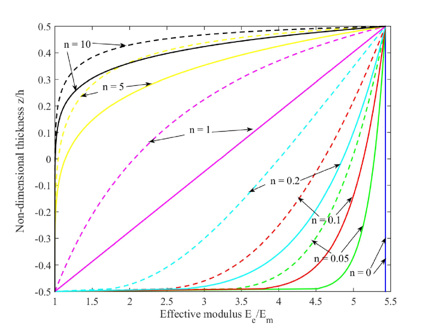
Figure 2: The effective modulus of Al/Al₂O₃ plates according to the rule of mixtures scheme (in solid lines) and Mori-Tanaka scheme (in dash lines).

2.3 A novel seventh-order shear deformation plate theory

With regard to the plate theories, the third-order shear deformation model initially proposed by Reddy [52] is widely considered as a reliable theory in which no shear correction factor is required. In Reddy’s theory, the displacement field, for $z\in\left[{-h/2;h/2}\right]$, is defined as

$$u\left({x,y,z}\right) =u_{0}\left({x,y}\right)+z\beta_{x}\left({x,y}\right)+g\left(z\right)\left({\beta_{x}\left({x,y}\right)+w_{,x}\left({x,y}\right)}\right),$$ (11a)

$$v\left({x,y,z}\right) =v_{0}\left({x,y}\right)+z\beta_{y}\left({x,y}\right)+g\left(z\right)\left({\beta_{y}\left({x,y}\right)+w_{,y}\left({x,y}\right)}\right),$$ (11b)

$$w\left({x,y,z}\right) =w_{0}\left({x,y}\right),$$ (11c)

where comma notation represents derivative, $g(z)=-4z^{3}/(3h^{2})$ and the variables ${\bf{u}}_{0}=\left[{u_{0}\quad v_{0}}\right]^{T}$, $w_{0}$, and ${\boldsymbol{\beta}}=\left[{\beta_{x}\quad\beta_{y}}\right]^{T}$ are the membrane displacements, the transverse deflection of the mid-plane surface, and the rotations, respectively. By making further assumptions, $w_{0}=w_{b}+w_{s},\beta_{x}=-w_{b,x},\beta_{y}=-w_{b,y}$, to the Reddy’s theory which contains five unknowns, Senthilnathan [55] initially proposes the four-variable refined plate theory which could be expressed in the generalized form as follows

$$u\left({x,y,z}\right) =u_{0}\left({x,y}\right)-zw_{b,x}\left({x,y}\right)+g\left(z\right)w_{s,x}\left({x,y}\right),$$ (12a)

$$v\left({x,y,z}\right) =v_{0}\left({x,y}\right)-zw_{b,y}\left({x,y}\right)+g\left(z\right)w_{s,y}\left({x,y}\right),$$ (12b)

$$w\left({x,y,z}\right) =w_{b}\left({x,y}\right)+w_{s}\left({x,y}\right),$$ (12c)

where $w_{b}$ and $w_{s}$ represent bending and shear components of transverse displacement, respectively. The function $g(z)=f(z)-z$ is employed to describe the distribution of transverse shear strains and stresses through the plates’ thickness. It is necessary to have the first derivative of $f(z)$ satisfies the tangential zero value at $z=\pm h/2$ such that the traction-free condition at top and bottom surfaces is meet. Consequently, the shear correction factor is no longer required for higher-order shear deformation theory and refined plate theory.

It should be noted that the higher-order shear deformation theory and refined plate theory both fail to capture the thickness stretching effect of normal deformation $(\varepsilon_{z}\neq 0)$ due to the constant deflection through the plate thickness which can be inferred from Eq. (12c). In order to bypass this shortcoming, a number of theories which consider the thickness stretching effect have been developed [78, 79, 80]. Zenkour [81, 82] initially proposes the four-variable quasi-3D plate theory accounting for both transverse shear and normal deformations which could be alternatively expressed as follows

$$u\left({x,y,z}\right) =u_{0}\left({x,y}\right)-zw_{b,x}\left({x,y}\right)+f\left(z\right)w_{s,x}\left({x,y}\right),$$ (13a)

$$v\left({x,y,z}\right) =v_{0}\left({x,y}\right)-zw_{b,y}\left({x,y}\right)+f\left(z\right)w_{s,y}\left({x,y}\right),$$ (13b)

$$w\left({x,y,z}\right) =w_{b}\left({x,y}\right)+\phi\left(z\right)w_{s}\left({x,y}\right).$$ (13c)

As can be observed, this quasi-3D model has a similar form to that of four-variable refined plate theory shown in Eq. (12). Indeed, the displacement field based on the refined plate theory could be readily obtained by degrading those of quasi-3D theory in which $f(z)$ and $\phi(z)$ are replaced by $g(z)$ and $1$, respectively.

A number of distribution functions, $f(z)$ and $\phi(z)$, are available to analyse the FGM plates based on higher-order shear deformation theory, refined plate theory, and quasi-3D plate theory. One may find the general framework to construct such polynomial functions in the recent work of Nguyen et al. [83]. In this study, a novel seventh-order function of $f(z)$ and corresponding function $\phi(z)$ are proposed for the four-variable refined plate theory and quasi-3D theory. Those functions are presented in Table 1 along with other’s existing in the literature.

Table 1: Various forms of distribution function used for HSDT, RPT, and quasi-3D theories

Theory	$\varepsilon_{z}$	$f(z)$	$\phi_{z}$
HSDT [52]	$=0$	$z-\frac{4}{3}\frac{{z^{3}}}{{h^{2}}}$	-
RPT [61]	$=0$	$\arctan\left({\sin\left({\frac{\pi}{h}z}\right)}\right)$	-
Quasi-3D [91]	$\neq 0$	$\frac{h}{\pi}\sin\left({\frac{{\pi z}}{h}}\right)-z$	$f^{\prime}\left(z\right)+1$
Quasi-3D [81]	$\neq 0$	$h\sinh\left({\frac{z}{h}}\right)-\frac{{4z^{3}}}{{3h^{2}}}\cosh\left({\frac{1}{2}}\right)$	$\frac{1}{{12}}f^{\prime}\left(z\right)$
Quasi-3D [85]	$\neq 0$	$\frac{\pi}{h}z-\frac{{9\pi}}{{5h^{3}}}z^{3}+\frac{{28\pi}}{{25h^{5}}}z^{5}$	$\frac{1}{8}f^{\prime}\left(z\right)$
Present RPT	$=0$	$-8z+\frac{{10z^{3}}}{{h^{2}}}+\frac{{6z^{5}}}{{5h^{4}}}+\frac{{8z^{7}}}{{7h^{6}}}$	-
Present quasi-3D	$\neq 0$	$-8z+\frac{{10z^{3}}}{{h^{2}}}+\frac{{6z^{5}}}{{5h^{4}}}+\frac{{8z^{7}}}{{7h^{6}}}$	$\frac{3}{{20}}f^{\prime}\left(z\right)$

According to the displacement field and the strain-displacement relation, which are presented in Eqs. (13) and (2a), respectively, the following strain expressions could be obtained as

$$\boldsymbol{{\bf{\varepsilon}}} =\boldsymbol{{\bf{\varepsilon}}}_{0}+z{\boldsymbol{\kappa}}_{b}+f\left(z\right){\boldsymbol{\kappa}}_{s},$$ (14a)

$$\boldsymbol{\bf{\gamma}} =\left[{f^{\prime}\left(z\right)+\phi\left(z\right)}\right]\boldsymbol{{\bf{\varepsilon}}}_{s},$$ (14b)

where

$$\begin{split}\boldsymbol{{\bf{\varepsilon}}}&=\left[\begin{array}[]{l}\varepsilon_{x}\\ \varepsilon_{y}\\ \gamma_{xy}\\ \end{array}\right],\quad\boldsymbol{{\bf{\varepsilon}}}_{0}=\left[\begin{array}[]{l}u_{0,x}\\ v_{0,y}\\ u_{0,y}+v_{0,x}\\ \end{array}\right],\quad{\boldsymbol{\kappa}}_{b}=-\left[\begin{array}[]{l}w_{b,xx}\\ w_{b,yy}\\ 2w_{b,xy}\\ \end{array}\right],\quad{\boldsymbol{\kappa}}_{s}=\left[\begin{array}[]{l}w_{s,xx}\\ w_{s,yy}\\ 2w_{s,xy}\\ \end{array}\right],\\ \boldsymbol{\bf{\gamma}}&=\left[\begin{array}[]{l}\gamma_{xz}\\ \gamma_{yz}\\ \end{array}\right],\quad\boldsymbol{\bf{\varepsilon}}_{s}=\left[\begin{array}[]{l}w_{s,x}\\ w_{s,y}\\ \end{array}\right],\quad\varepsilon_{z}=\phi^{\prime}\left(z\right)w_{s}.\end{split}$$ (15)

Using Eqs. (13), (3), and (2b), rotation vector and curvature vector are respectively expressed by

$$\boldsymbol{\theta} =\left[\begin{array}[]{l}\theta_{x}\\ \theta_{y}\\ \theta_{z}\\ \end{array}\right]=\frac{1}{2}\left[\begin{array}[]{l}2w_{b,y}-\left({f^{\prime}-\phi}\right)w_{s,y}\\ -2w_{b,x}+\left({f^{\prime}-\phi}\right)w_{s,x}\\ v_{0,x}-u_{0,y}\\ \end{array}\right],$$ (16g)

$${\boldsymbol{\chi}} =\left[\begin{array}[]{l}{\boldsymbol{\chi}}_{b}\\ {\boldsymbol{\chi}}_{s}\\ \chi_{zz}\\ \end{array}\right]=\left[\begin{array}[]{l}{\boldsymbol{\chi}}_{b0}\\ {\boldsymbol{\chi}}_{s0}\\ 0\\ \end{array}\right]+\left[\begin{array}[]{l}f^{\prime}{\boldsymbol{\chi}}_{b1}\\ f^{\prime\prime}{\boldsymbol{\chi}}_{s2}\\ 0\\ \end{array}\right]+\left[\begin{array}[]{l}\phi{\boldsymbol{\chi}}_{b3}\\ \phi^{\prime}{\boldsymbol{\chi}}_{s4}\\ 0\\ \end{array}\right],$$ (16t)

where

$$\begin{split}{\boldsymbol{\chi}}_{b}&=\left[\begin{array}[]{l}\chi_{xx}\\ \chi_{yy}\\ \chi_{xy}\\ \end{array}\right],{\boldsymbol{\chi}}_{b0}=\frac{1}{2}\left[\begin{array}[]{l}w_{b,xy}\\ -w_{b,xy}\\ w_{b,yy}-w_{b,xx}\\ \end{array}\right],{\boldsymbol{\chi}}_{b1}=\frac{1}{4}\left[\begin{array}[]{l}-2w_{s,xy}\\ 2w_{s,xy}\\ -w_{s,yy}+w_{s,xx}\\ \end{array}\right],{\boldsymbol{\chi}}_{b3}=\frac{1}{4}\left[\begin{array}[]{l}2w_{s,xy}\\ -2w_{s,xy}\\ w_{s,yy}-w_{s,xx}\\ \end{array}\right],\\ {\boldsymbol{\chi}}_{s}&=\left[\begin{array}[]{l}\chi_{xz}\\ \chi_{yz}\\ \end{array}\right],{\boldsymbol{\chi}}_{s0}=\frac{1}{4}\left[\begin{array}[]{l}v_{0,xx}-u_{0,xy}\\ v_{0,xy}-u_{0,yy}\\ \end{array}\right],{\boldsymbol{\chi}}_{s2}=\frac{1}{4}\left[\begin{array}[]{l}-w_{s,y}\\ w_{s,x}\\ \end{array}\right],{\boldsymbol{\chi}}_{s4}=\frac{1}{4}\left[\begin{array}[]{l}w_{s,y}\\ -w_{s,x}\\ \end{array}\right].\end{split}$$ (17)

According to Eq. (5), the constitutive relations for classical and modified couple stress theories could be presented in explicit form as follows

$$\left\{\begin{array}[]{l}\sigma_{x}\\ \sigma_{y}\\ \sigma_{z}\\ \sigma_{xy}\\ \tau_{xz}\\ \tau_{yz}\\ \end{array}\right\} =\left[{\begin{array}[]{*{20}c}{Q_{11}}&{Q_{12}}&{Q_{13}}&0&0&0\\ {}\hfil&{Q_{22}}&{Q_{23}}&0&0&0\\ {}\hfil&{}\hfil&{Q_{33}}&0&0&0\\ {}\hfil&{}\hfil&{}\hfil&{Q_{66}}&0&0\\ {}\hfil&{}\hfil&{}\hfil&{}\hfil&{Q_{55}}&0\\ {\text{sym.}}&{}\hfil&{}\hfil&{}\hfil&{}\hfil&{Q_{44}}\\ \end{array}}\right]\left\{\begin{array}[]{l}\varepsilon_{x}\\ \varepsilon_{y}\\ \varepsilon_{z}\\ \varepsilon_{xy}\\ \gamma_{xz}\\ \gamma_{yz}\\ \end{array}\right\},$$ (18s)

$$m_{ij} =2G_{e}l^{2}\chi_{ij},$$ (18t)

where, for the proposed quasi-3D theory $(\varepsilon_{z}\neq 0)$, $Q_{ij}$ are the three-dimensional elastic constant which could be calculated as

$$\begin{split}Q_{11}&=Q_{22}=Q_{33}=\frac{{\left({1-\nu_{e}}\right)E_{e}}}{{\left({1-2\nu_{e}}\right)\left({1+\nu_{e}}\right)}},\\ Q_{12}&=Q_{13}=Q_{23}=\frac{{\nu_{e}E_{e}}}{{\left({1-2\nu_{e}}\right)\left({1+\nu_{e}}\right)}},\\ Q_{44}&=Q_{55}=Q_{66}=\frac{{E_{e}}}{{2\left({1+\nu_{e}}\right)}},\end{split}$$ (19)

meanwhile, for the proposed refined plate theory $(\varepsilon_{z}=0)$, $Q_{ij}$ are reduced plane-stress elastic constant and are expressed as

$$\begin{split}Q_{11}&=Q_{22}=\frac{{E_{e}}}{{1-\nu_{e}^{2}}},\\ Q_{12}&=Q_{21}=\frac{{E_{e}\nu_{e}}}{{1-\nu_{e}^{2}}},\\ Q_{44}&=Q_{55}=Q_{66}=\frac{{E_{e}}}{{2\left({1+\nu_{e}}\right)}},\end{split}$$ (20)

and the shear modulus $G_{e}=\dfrac{E_{e}}{2(1+\nu_{e})}$.

In this study, the weak form of the static bending, vibration, and buckling problems are derived using the Hamilton’s principle and weak formulation. One could find those straightforward procedures in the literature [84, 61, 85]. Firstly, the weak form of the static bending of the couple-stress-based microplates subjected to transverse load loading $q_{0}$ could be expressed in the following compact form

$$\begin{split}\int\limits_{\Omega}{\delta{\boldsymbol{\bf{\varepsilon}}}_{b}^{T}{\bf{D}}^{b}{\boldsymbol{\bf{\varepsilon}}}_{b}d\Omega}+\int\limits_{\Omega}{\delta{\boldsymbol{\bf{\varepsilon}}}_{s}^{T}{\bf{D}}^{s}{\boldsymbol{\bf{\varepsilon}}}_{s}d\Omega}+\int\limits_{\Omega}{\delta\left({{\boldsymbol{\chi}}_{b}^{c}}\right)^{T}{\boldsymbol{D}}_{c}^{b}{\boldsymbol{\chi}}_{b}^{c}d\Omega}+\int\limits_{\Omega}{\delta\left({{\boldsymbol{\chi}}_{s}^{c}}\right)^{T}{\bf{D}}_{c}^{s}{\boldsymbol{\chi}}_{s}^{c}d\Omega}\\ =\int\limits_{\Omega}{\left[{\delta w_{b}+\phi\left({\frac{h}{2}}\right)\delta w_{s}}\right]q_{0}d\Omega}\end{split},$$ (21)

where the strain tensors and matrices in the first two terms in Eq. (21) related to classical elastic theory are

$${\boldsymbol{\boldsymbol{\varepsilon}}}_{b}=\left[\begin{array}[]{l}{\bf{\varepsilon}}_{0}\\ {\bf{\kappa}}_{b}\\ {\bf{\kappa}}_{s}\\ w_{s}\\ \end{array}\right],\quad{\boldsymbol{\boldsymbol{\varepsilon}}}_{s}=\left[\begin{array}[]{l}w_{s,x}\\ w_{s,y}\\ \end{array}\right],\quad{\bf{D}}^{b}=\left[{\begin{array}[]{*{20}c}{\bf{A}}&{\bf{B}}&{\bf{E}}&{\bf{X}}\\ {\bf{B}}&{\bf{D}}&{\bf{F}}&{{\bf{Y}}^{b}}\\ {\bf{E}}&{\bf{F}}&{\bf{H}}&{{\bf{Y}}^{s}}\\ {\bf{X}}&{{\bf{Y}}^{b}}&{{\bf{Y}}^{s}}&{Z_{33}}\\ \end{array}}\right],$$ (22)

in which the material matrices are calculated by

$$\left({{\bf{A}},{\bf{B}},{\bf{D}},{\bf{E}},{\bf{F}},{\bf{H}}}\right)=\int\limits_{-h/2}^{h/2}{\left[{1,z,z^{2},f\left(z\right),zf\left(z\right),f^{2}\left(z\right)}\right]\,{\bar{\bf Q}}dz},$$ (23a)

$$\left({{\bf{X}},{\bf{Y}}^{b},{\bf{Y}}^{s}}\right)=\int\limits_{-h/2}^{h/2}{\left[{\phi^{\prime}\left(z\right),z\phi^{\prime}\left(z\right),f\left(z\right)\phi^{\prime}\left(z\right)}\right]\,{\tilde{\bf Q}}dz},$$ (23b)

$$Z_{33}=\int\limits_{-h/2}^{h/2}{\left[{\phi^{\prime}\left(z\right)}\right]^{2}\,Q_{33}dz},$$ (23c)

$${\bf{D}}^{s}=\int\limits_{-h/2}^{h/2}{\left[{f^{\prime}\left(z\right)+\phi\left(z\right)}\right]^{2}{\hat{\bf Q}}dz},$$ (23d)

$${\bf{\bar{Q}}}=\left[{\begin{array}[]{*{20}c}{Q_{11}}&{Q_{12}}&0\\ {Q_{21}}&{Q_{22}}&0\\ 0&0&{Q_{66}}\\ \end{array}}\right],\quad{\tilde{\bf Q}}=\left[{\begin{array}[]{*{20}c}{Q_{13}}\\ {Q_{23}}\\ 0\\ \end{array}}\right],\quad{\hat{\bf Q}}=\left[{\begin{array}[]{*{20}c}{Q_{44}}&0\\ 0&{Q_{55}}\\ \end{array}}\right],$$ (23m)

and where the curvature tensors and matrices in the third and fourth terms in Eq. (21) representing the couple stress theory are

$${\boldsymbol{\chi}}_{b}^{c}=\left[\begin{array}[]{l}{\boldsymbol{\chi}}_{b0}\\ {\boldsymbol{\chi}}_{b1}\\ {\boldsymbol{\chi}}_{b3}\\ \end{array}\right],\quad{\boldsymbol{\chi}}_{s}^{c}=\left[\begin{array}[]{l}{\boldsymbol{\chi}}_{s0}\\ {\boldsymbol{\chi}}_{s2}\\ {\boldsymbol{\chi}}_{s4}\\ \end{array}\right],\quad{\bf{D}}_{c}^{b}=\left[{\begin{array}[]{*{20}c}{{\bf{A}}^{c}}&{{\bf{B}}^{c}}&{{\bf{E}}^{c}}\\ {{\bf{B}}^{c}}&{{\bf{D}}^{c}}&{{\bf{F}}^{c}}\\ {{\bf{E}}^{c}}&{{\bf{F}}^{c}}&{{\bf{H}}^{c}}\\ \end{array}}\right],\quad{\bf{D}}_{c}^{s}=\left[{\begin{array}[]{*{20}c}{{\bf{X}}^{c}}&{{\bf{Y}}^{c}}&{{\bf{T}}^{c}}\\ {{\bf{Y}}^{c}}&{{\bf{Z}}^{c}}&{{\bf{V}}^{c}}\\ {{\bf{T}}^{c}}&{{\bf{V}}^{c}}&{{\bf{W}}^{c}}\\ \end{array}}\right],$$ (24)

in which the material matrices could be defined as

$$\left({{\bf{A}}^{c},{\bf{B}}^{c},{\bf{D}}^{c},{\bf{E}}^{c},{\bf{F}}^{c},{\bf{H}}^{c}}\right) =\int\limits_{-h/2}^{h/2}{\left({1,f^{\prime}\left(z\right),\left[{f^{\prime}\left(z\right)}\right]^{2},\phi\left(z\right),f^{\prime}\left(z\right)\phi\left(z\right),\left[{\phi\left(z\right)}\right]^{2}}\right)\,{\bar{\bf G}}dz},$$ (25a)

$$\left({{\bf{X}}^{c},{\bf{Y}}^{c},{\bf{Z}}^{c},{\bf{T}}^{c},{\bf{V}}^{c},{\bf{W}}^{c}}\right)\, =\int\limits_{-h/2}^{h/2}{\left({1,f^{\prime\prime}\left(z\right),\left[{f^{\prime\prime}\left(z\right)}\right]^{2},\phi^{\prime}\left(z\right),f^{\prime\prime}\left(z\right)\phi^{\prime}\left(z\right),\left[{\phi^{\prime}\left(z\right)}\right]^{2}}\right)\,{\hat{\bf G}}dz},$$ (25b)

where

$${\bar{\bf G}}=2G_{e}l^{2}\left[{\begin{array}[]{*{20}c}1&0&0\\ 0&1&0\\ 0&0&1\\ \end{array}}\right],\quad{\hat{\bf G}}=2G_{e}l^{2}\left[{\begin{array}[]{*{20}c}1&0\\ 0&1\\ \end{array}}\right].$$ (26)

The weak form of the free vibration of the couple-stress-based microplates is briefly expressed as

$$\int\limits_{\Omega}{\boldsymbol{\delta{\bf{\varepsilon}}}_{b}^{T}{\bf{D}}^{b}{\boldsymbol{\bf{\varepsilon}}}_{b}d\Omega}+\int\limits_{\Omega}{\delta{\boldsymbol{\bf{\varepsilon}}}_{s}^{T}{\bf{D}}^{s}{\boldsymbol{\bf{\varepsilon}}}_{s}d\Omega}+\int\limits_{\Omega}{\delta\left({{\boldsymbol{\chi}}_{b}^{c}}\right)^{T}{\bf{D}}_{c}^{b}{\boldsymbol{\chi}}_{b}^{c}d\Omega}+\int\limits_{\Omega}{\delta\left({{\boldsymbol{\chi}}_{s}^{c}}\right)^{T}{\bf{D}}_{c}^{s}{\boldsymbol{\chi}}_{s}^{c}d\Omega}=\int\limits_{\Omega}{\delta{\tilde{\bf u}}^{T}{\tilde{{\bf{m}}}}\ddot{\tilde{{\bf{u}}}}d\Omega},$$ (27)

where $\tilde{{\bf{u}}}=\left[{u_{0}\quad-w_{b,x}\quad w_{s,x}\quad v_{0}\quad-w_{b,y}\quad w_{s,y}\quad w_{b}\quad w_{s}\quad 0}\right]^{T}$, and the mass matrix $\tilde{{\bf{m}}}$ is defined by

$${\tilde{\bf m}}=\left[{\begin{array}[]{*{20}c}{{\bf{I}}_{0}}&0&0\\ 0&{{\bf{I}}_{0}}&0\\ 0&0&{{\bf{I}}_{1}}\\ \end{array}}\right]\quad\text{in which}\quad{\bf{I}}_{0}=\left[{\begin{array}[]{*{20}c}{I_{1}}&{I_{2}}&{I_{4}}\\ {I_{2}}&{I_{3}}&{I_{5}}\\ {I_{4}}&{I_{5}}&{I_{6}}\\ \end{array}}\right],\quad{\bf{I}}_{1}=\left[{\begin{array}[]{*{20}c}{I_{1}}&{I_{7}}&0\\ {I_{7}}&{I_{8}}&0\\ 0&0&0\\ \end{array}}\right],$$ (28j)

$$\left({I_{1},I_{2},I_{3},I_{4},I_{5},I_{6},I_{7},I_{8}}\right)=\int\limits_{-h/2}^{h/2}{\rho\left[{1,z,z^{2},f\left(z\right),zf\left(z\right),f^{2}\left(z\right),\phi\left(z\right),\phi^{2}\left(z\right)}\right]dz}.$$ (28k)

For buckling analysis, the weak form of the couple-stress-based microplates subjected to in-plane loading is of the form

$$\begin{split}\int\limits_{\Omega}{\delta{\boldsymbol{\bf{\varepsilon}}}_{b}^{T}{\bf{D}}^{b}{\boldsymbol{\bf{\varepsilon}}}_{b}d\Omega}+\int\limits_{\Omega}{\delta{\boldsymbol{\bf{\varepsilon}}}_{s}^{T}{\bf{D}}^{s}{\boldsymbol{\bf{\varepsilon}}}_{s}d\Omega}+\int\limits_{\Omega}{\delta\left({{\boldsymbol{\chi}}_{b}^{c}}\right)^{T}{\bf{D}}_{c}^{b}{\boldsymbol{\chi}}_{b}^{c}d\Omega}+\int\limits_{\Omega}{\delta\left({{\boldsymbol{\chi}}_{s}^{c}}\right)^{T}{\bf{D}}_{c}^{s}{\boldsymbol{\chi}}_{s}^{c}d\Omega}\\ +\int\limits_{\Omega}{\nabla^{T}\delta\left[{w_{b}+\phi\left(0\right)w_{s}}\right]{\bf{N}}_{0}\nabla\left[{w_{b}+\phi\left(0\right)w_{s}}\right]d\Omega}=0\end{split},$$ (29)

where $\nabla^{T}=\left[{\partial/\partial x\quad\partial/\partial y}\right]^{T}$ and ${\bf{N}}_{0}=\left[{\begin{array}[]{*{20}c}{N_{x}^{0}}&{N_{xy}^{0}}\\ {N_{xy}^{0}}&{N_{y}^{0}}\\ \end{array}}\right]$ are the transpose of gradient operator and matrix of pre-buckling loads, respectively.

3 FG microplate formulation based on NURBS basis functions

In this section, briefing review on NURBS which are served as the basis functions of isogeometric analysis will be presented. It is followed by a novel NURBS-based formulation for couple-stress microplate bending, free vibration and buckling that are relied on refined plate theory and quasi-3D theory.

3.1 B-splines and NURBS basis functions

The starting point of the NURBS basis functions is non-decreasing knot vector ${\bf{\Xi}}=\left\{{\xi_{1},\xi_{2},...,\xi_{n+p+1}}\right\}$ where the $i^{th}$ knot $\xi_{i}\in\mathbb{R}$, $n$ represents the number of basis functions, and $p$ denotes the polynomial order. The knot vectors could be either uniform if the knots are equally spaced in the parameter space or open if its first and last knot’s values are repeated $p+1$ times. The knot spans which are bounded by knots defines element domain. The B-spline basis functions that are constructed by the Cox-de Boor recursion formula, starting with the zeroth order ($p=0$) are defined by [60, 86]

$$N_{i,0}\left(\xi\right) =\left\{\begin{array}[]{l}1\quad\text{if}\quad\xi_{i}\leq\xi<\xi_{i+1},\\ 0\quad\text{otherwise,}\\ \end{array}\right.$$ (30c)

$$N_{i,p}\left(\xi\right) =\frac{{\xi-\xi_{i}}}{{\xi_{i+p}-\xi_{i}}}N_{i,p-1}\left(\xi\right)+\frac{{\xi_{i+p+1}-\xi}}{{\xi_{i+p+1}-\xi_{i+1}}}N_{i+1,p-1}\left(\xi\right),\text{for $p\geq 1$},$$ (30d)

in which the fraction $0/0$ is defined as zero. While the basis functions are smooth, e.g. $C^{\infty}$ continuity, within this domain, they are $C^{p-m}$ continuity across the knots, where $m$ is the multiplicity of the knot. Therefore, for $p\geq 2$, the basis functions would be of C¹ continuity at single knot and knot span as well. Two-dimensional B-splines are obtained by introducing the second knot vector ${{\bf{H}}}=\left\{{\eta_{1},\eta_{2},...,\eta_{m+q+1}}\right\}$ and using tensor product of $\bf{\Xi}$ and ${{\bf{H}}}$ in the parametric dimensions yielding

$$N_{A}\left({\xi,\eta}\right)=N_{i,p}\left(\xi\right)M_{j,q}\left(\eta\right).$$ (31)

For the illustration purposes, Fig. 3 depicts the one- and two-dimensional B-spline basis functions which are generated from the knot vector ${\bf{\Xi}}=\{0,0,0,0,1/5,2/5,3/5,3/5,3/5,4/5,1,1,1,1\}$ and its combination with the knot vector ${\bf{H}}=\{0,0,0,1/4,1/2,3/4,1,1,1\}$, respectively. The non-uniform rational B-splines (NURBS) basis functions are then further defined by providing additional weight $\zeta_{A}$ to each control point given by [86]

$$R_{A}\left({\xi,\eta}\right)=\frac{{N_{A}\zeta_{A}}}{{\sum\limits_{\hat{A}}^{m\times n}{N_{\hat{A}}\left({\xi,\eta}\right)\zeta_{\hat{A}}}}}.$$ (32)

It is noted that the B-spline basis function is served as a special case of the NURBS function. Indeed, if all the individual weights corresponding the control points are assigned an equal constant, the NURBS function yields B-spline function.

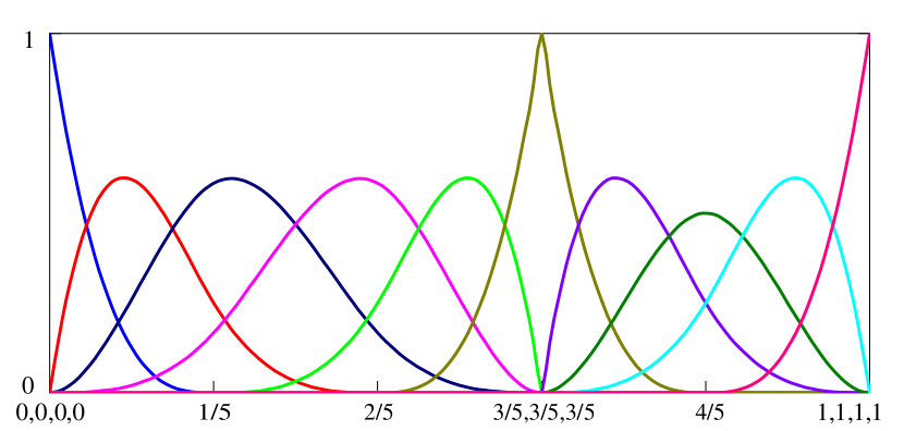
(a) Cubic basis functions corresponding to ${\boldsymbol{\Xi}}=\{0,0,0,0,\dfrac{1}{5},\dfrac{2}{5},\dfrac{3}{5},\dfrac{3}{5},\dfrac{3}{5},\dfrac{4}{5},1,1,1,1\}$.

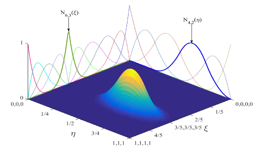
(b) Bivariate B-spline basis functions.

Figure 3: One- and two-dimensional B-spline basis functions.

3.2 A novel NURBS-based formulation of modified couple stress theory

By using the NURBS basis functions, the displacement variables $\bf{u}$ of a microplate could be approximately calculated as follows

$${\bf{u}}^{h}\left({\xi,\eta}\right)=\sum\limits_{A=1}^{n\times m}{R_{A}\left({\xi,\eta}\right)}{\bf{q}}_{A},$$ (33)

where $n\times m$ is the number of basis functions and ${\bf{q}}_{A}=[u_{0A}\quad v_{0A}\quad w_{bA}\quad w_{sA}]^{T}$ denotes the vector of degrees of freedom associated with the control point A. By substituting the variable approximations Eq. (33) into the strain-displacement relations Eq. (15), the in-plane and shear strains could be obtained as follows

$$\left[{{\boldsymbol{\varepsilon}}_{0}^{T}\quad{\boldsymbol{\kappa}}_{b}^{T}\quad{\boldsymbol{\kappa}}_{s}^{T}\quad{\boldsymbol{\varepsilon}}_{s}^{T}}\right]^{T}=\sum\limits_{A=1}^{n\times m}{\left[{\left({{\bf{B}}_{A}^{m}}\right)^{T}\quad\left({{\bf{B}}_{A}^{b1}}\right)^{T}\quad\left({{\bf{B}}_{A}^{b2}}\right)^{T}\quad\left({{\bf{B}}_{A}^{s}}\right)^{T}}\right]^{T}{\bf{q}}_{A}},$$ (34)

where

$$\begin{split}{\bf{B}}_{A}^{m}&=\left[{\begin{array}[]{*{20}c}{R_{A,x}}&0&0&0\\ 0&{R_{A,y}}&0&0\\ {R_{A,y}}&{R_{A,x}}&0&0\\ \end{array}}\right],\quad{\bf{B}}_{A}^{b1}=-\left[{\begin{array}[]{*{20}c}0&0&{R_{A,xx}}&0\\ 0&0&{R_{A,yy}}&0\\ 0&0&{2R_{A,xy}}&0\\ \end{array}}\right],\\ {\bf{B}}_{A}^{b2}&=\left[{\begin{array}[]{*{20}c}0&0&0&{R_{A,xx}}\\ 0&0&0&{R_{A,yy}}\\ 0&0&0&{2R_{A,xy}}\\ \end{array}}\right],\quad{\bf{B}}_{A}^{s}=\left[{\begin{array}[]{*{20}c}0&0&0&{R_{A,x}}\\ 0&0&0&{R_{A,y}}\\ \end{array}}\right],\end{split}$$ (35)

and the curvatures could be obtained by substituting Eq. (33) into Eq. (17) :

$$\begin{split}&\left[{{\boldsymbol{\chi}}_{b0}^{T}\quad{\boldsymbol{\chi}}_{b1}^{T}\quad{\boldsymbol{\chi}}_{b3}^{T}\quad{\boldsymbol{\chi}}_{s0}^{T}\quad{\boldsymbol{\chi}}_{s2}^{T}\quad{\boldsymbol{\chi}}_{s4}^{T}}\right]^{T}\\ &=\sum\limits_{A=1}^{n\times m}{\left[{\left({{\tilde{\bf B}}_{A}^{b0}}\right)^{T}\quad\left({{\tilde{\bf B}}_{A}^{b1}}\right)^{T}\quad\left({{\tilde{\bf B}}_{A}^{b3}}\right)^{T}\quad\left({{\tilde{\bf B}}_{A}^{s0}}\right)^{T}\quad\left({{\tilde{\bf B}}_{A}^{s2}}\right)^{T}\quad\left({{\tilde{\bf B}}_{A}^{s4}}\right)^{T}}\right]^{T}{\bf{q}}_{A}},\end{split}$$ (36)

where

$$\begin{split}{\tilde{\bf B}}_{A}^{b0}&=\frac{1}{2}\left[{\begin{array}[]{*{20}c}0&0&{2R_{A,xy}}&0\\ 0&0&{-2R_{A,xy}}&0\\ 0&0&{\left({-R_{A,xx}+R_{A,yy}}\right)}&0\\ \end{array}}\right],\quad{\tilde{\bf B}}_{A}^{b1}=\frac{1}{4}\left[{\begin{array}[]{*{20}c}0&0&0&{-2R_{A,xy}}\\ 0&0&0&{2R_{A,xy}}\\ 0&0&0&{\left({R_{A,xx}-R_{A,yy}}\right)}\\ \end{array}}\right],\\ {\tilde{\bf B}}_{A}^{b3}&=\frac{1}{4}\left[{\begin{array}[]{*{20}c}0&0&0&{2R_{A,xy}}\\ 0&0&0&{-2R_{A,xy}}\\ 0&0&0&{\left({-R_{A,xx}+R_{A,yy}}\right)}\\ \end{array}}\right],\quad{\tilde{\bf B}}_{A}^{s0}=\frac{1}{4}\left[{\begin{array}[]{*{20}c}{-R_{A,xy}}&{R_{A,xx}}&0&0\\ {-R_{A,yy}}&{R_{A,xy}}&0&0\\ \end{array}}\right],\\ {\tilde{\bf B}}_{A}^{s2}&=\frac{1}{4}\left[{\begin{array}[]{*{20}c}0&0&0&{-R_{A,y}}\\ 0&0&0&{R_{A,x}}\\ \end{array}}\right],\quad{\tilde{\bf B}}_{A}^{s4}=\frac{1}{4}\left[{\begin{array}[]{*{20}c}0&0&0&{R_{A,y}}\\ 0&0&0&{-R_{A,x}}\\ \end{array}}\right].\end{split}$$ (37)

Substituting Eqs. (34) and (36) into Eqs. (21), (27), and (29), the matrix form of the global equilibrium equations for static bending, free vibration, and buckling could be respectively presented by

$${\bf{Kq}} ={\bf{F}},$$ (38a)

$$\left({{\bf{K}}-{\bf{\omega}}^{2}{\bf{M}}}\right){\bf{q}} ={\bf{0}},$$ (38b)

$$\left({{\bf{K}}-{\bf{\lambda}}_{cr}{\bf{K}}_{g}}\right){\bf{q}} ={\bf{0}},$$ (38c)

where the global stiffness matrix $\bf{K}$ is the summation of the stiffness matrices corresponding to the classical theory ${\bf{K}}_{s}$ and the couple stress theory ${\bf{K}}_{c}$, i.e. ${\bf{K}}={\bf{K}}_{s}+{\bf{K}}_{c}$. These matrices are calculated as follow

$${\bf{K}}_{s} =\int\limits_{\Omega}{\left({\left\{\begin{array}[]{l}{\bf{B}}^{m}\\ {\bf{B}}^{b1}\\ {\bf{B}}^{b2}\\ {\bf{B}}^{z}\\ \end{array}\right\}^{T}\left[{\begin{array}[]{*{20}c}{\bf{A}}&{\bf{B}}&{\bf{E}}&{\bf{X}}\\ {\bf{B}}&{\bf{D}}&{\bf{F}}&{{\bf{Y}}^{b}}\\ {\bf{E}}&{\bf{F}}&{\bf{H}}&{{\bf{Y}}^{s}}\\ {\bf{X}}&{{\bf{Y}}^{b}}&{{\bf{Y}}^{s}}&{Z_{33}}\\ \end{array}}\right]\left\{\begin{array}[]{l}{\bf{B}}^{m}\\ {\bf{B}}^{b1}\\ {\bf{B}}^{b2}\\ {\bf{B}}^{z}\\ \end{array}\right\}+\left({{\bf{B}}^{s}}\right)^{T}{\bf{D}}^{s}{\bf{B}}^{s}}\right)d\Omega},$$ (39m)

$${\bf{K}}_{c} =\int\limits_{\Omega}{\left({\left\{\begin{array}[]{l}{\tilde{\bf B}}^{b0}\\ {\tilde{\bf B}}^{b1}\\ {\tilde{\bf B}}^{b3}\\ \end{array}\right\}^{T}\left[{\begin{array}[]{*{20}c}{{\bf{A}}^{c}}&{{\bf{B}}^{c}}&{{\bf{E}}^{c}}\\ {{\bf{B}}^{c}}&{{\bf{D}}^{c}}&{{\bf{F}}^{c}}\\ {{\bf{E}}^{c}}&{{\bf{F}}^{c}}&{{\bf{H}}^{c}}\\ \end{array}}\right]\left\{\begin{array}[]{l}{\tilde{\bf B}}^{b0}\\ {\tilde{\bf B}}^{b1}\\ {\tilde{\bf B}}^{b3}\\ \end{array}\right\}+\left\{\begin{array}[]{l}{\tilde{\bf B}}^{s0}\\ {\tilde{\bf B}}^{s2}\\ {\tilde{\bf B}}^{s4}\\ \end{array}\right\}^{T}\left[{\begin{array}[]{*{20}c}{{\bf{X}}^{c}}&{{\bf{Y}}^{c}}&{{\bf{T}}^{c}}\\ {{\bf{Y}}^{c}}&{{\bf{Z}}^{c}}&{{\bf{V}}^{c}}\\ {{\bf{T}}^{c}}&{{\bf{V}}^{c}}&{{\bf{W}}^{c}}\\ \end{array}}\right]\left\{\begin{array}[]{l}{\tilde{\bf B}}^{s0}\\ {\tilde{\bf B}}^{s2}\\ {\tilde{\bf B}}^{s4}\\ \end{array}\right\}}\right)d\Omega},$$ (39af)

in which ${\bf{B}}_{A}^{z}=\left[{\begin{array}[]{*{20}c}0&0&0&{R_{A}}\\ \end{array}}\right]$. The load vector $\bf{F}$ is given by

$${\bf{F}}=\int\limits_{\Omega}{q_{0}{\bf{R}}d\Omega},$$ (40)

where ${\bf{R}}=\left[{\begin{array}[]{*{20}c}0&0&{R_{A}}&{\phi\left({\frac{h}{2}}\right)R_{A}}\\ \end{array}}\right]^{T}$, the global mass matrix is computed by

$${\bf{M}}=\int\limits_{\Omega}{{\tilde{\bf R}}^{T}{\tilde{\bf m}}{\tilde{\bf R}}d\Omega},$$ (41)

in which

$$\begin{split}\tilde{\bf{R}}&=\left\{\begin{array}[]{l}{\bf{R}}_{1}\\ {\bf{R}}_{2}\\ {\bf{R}}_{3}\\ \end{array}\right\},\quad{\bf{R}}_{1}=\left[{\begin{array}[]{*{20}c}{R_{A}}&0&0&0\\ 0&0&{-R_{A,x}}&0\\ 0&0&0&{R_{A,x}}\\ \end{array}}\right],\\ {\bf{R}}_{2}&=\left[{\begin{array}[]{*{20}c}0&{R_{A}}&0&0\\ 0&0&{-R_{A,y}}&0\\ 0&0&0&{R_{A,y}}\\ \end{array}}\right],\quad{\bf{R}}_{3}=\left[{\begin{array}[]{*{20}c}0&0&{R_{A}}&0\\ 0&0&0&{R_{A}}\\ 0&0&0&0\\ \end{array}}\right],\end{split}$$ (42)

the geometric stiffness matrix is given as

$${\bf{K}}_{g}=\int\limits_{\Omega}{\left({{\bf{B}}^{g}}\right)}^{T}{\bf{N}}_{0}{\bf{B}}^{g}d\Omega,$$ (43)

where

$${\bf{B}}^{g}=\left[{\begin{array}[]{*{20}c}0&0&{R_{A,x}}&{\phi\left(0\right)R_{A,x}}\\ 0&0&{R_{A,y}}&{\phi\left(0\right)R_{A,y}}\\ \end{array}}\right],$$ (44)

and $\omega$ and $\lambda_{cr}$ represent the natural frequency and the critical buckling value, respectively.

As can be observed from Eq. (39), by introducing the distribution function $f(z)$, the four-variable refined plate theory and quasi-3D theory do not require any shear correction factor, which is usually needed if the first-order shear deformation theory is applied, to describe the transverse shear stresses satisfying traction-free conditions. In addition, the expressions of $\bf{B}$ and ${\tilde{\bf{B}}}$ matrices in Eqs. (35) and (37), respectively, show the employment of the second-order derivatives of the approximation functions $R_{A}$. Consequently, C¹-continuity approximations are required. This requirement may cause severe issues in finite element analysis which could only be solved by increasing the degrees of freedom resulting in higher number of variables and computational cost. However, within the platform of isogeometric analysis in which NURBS basis functions are employed, the C¹-continuity requirement could be naturally satisfied for $p\geq 2$ since the basis functions are C^p-1 continuous across the knot spans, i.e. elements.

4 Numerical examples and discussion

In this section, the convergence and verification studies are firstly conducted to demonstrate the validity and accuracy of the novel approaches presented in Section 2 and 3. In order to illustrate the efficiency of the IGA approach in dealing with modified couple stress theory, this section is then continued by the computational analysis of FG rectangular and circular microplates with various types of boundary condition for static bending, free vibration and buckling problems. In these investigations, the FG microplates made of mixtures of metal and ceramic whose material properties presented in Table 2 are used. Throughout the numerical examples, unless otherwise specified, the material length scale $l$ is chosen as $17.6\times 10^{-6}$m which was suggested by Lam et al. [20]. There are two types of boundary condition considered as follows

Simply supported (S)

$v_{0}=w_{b}=w_{s}=0$  at $x=0,a$

$u_{0}=w_{b}=w_{s}=0$  at $y=0,b$

Clamped (C)

$u_{0}=v_{0}=w_{b}=w_{s}=0$ and $w_{b,x}=w_{b,y}=w_{b,z}=w_{s,x}=w_{s,y}=w_{s,z}=0$

It should be noted that, within the IGA platform, while the homogeneous boundary conditions corresponded to displacement itself, e.g. $u_{0},v_{0},w_{b},w_{s}$, are easily treated in a similar way to the traditional finite element method, those require first derivative of displacement, e.g. $w_{b,x},w_{b,y},w_{b,z},w_{s,x},w_{s,y},w_{s,z}$, could be done by assigning zero values for all displacements of control points which are directly related to clamped edges and their adjacent points [87, 85].

Table 2: Material properties of FG plates

Property	Material
	Al	Al2O3	ZrO2-1	ZrO2-2
E (GPa)	70	380	200	151
$\nu$	0.3	0.3	0.3	0.3
$\rho$ (kg/m3)	2707	3800	3000	3000

4.1 Convergence and verification studies

In order to evaluate the convergence and reliability of the novel shape functions and IGA approach proposed in Section 2 and 3, the MCST-based size-dependent analysis of homogeneous fully simply-supported (SSSS) square microplate which is shown in Fig. 5 is conducted using RPT model. Moderately thick plates $(a/h=20)$ with four different values of material length scale ratio $(l/h=0,0.2,0.6,1)$ are investigated. For each case, eight different finite element meshes are analysed to study the convergence rate of the proposed IGA approach. As can be seen from Table 3, while fast convergence of the analysis for polynomial order $p=3$ and $p=4$ is archived, solutions using $p=2$ experience relatively slower convergence rate toward analytical solutions reported by Thai and Kim [43]. Fig. 4 presents the convergence study of non-dimensional central deflection of homogeneous square microplates with respect to the analytical solutions [43] for the case of $l/h=0.2$. Based on the convergence study, the cubic ($p=3$) NURBS element mesh of $11\times 11$ is relatively sufficient for all analysis cases. Therefore, this mesh whose geometry shown in Fig. 5 will be used throughout the next examples unless otherwise specified.

Table 3: Convergence of non-dimensional central deflection $\bar{w}=\dfrac{10Eh^{3}}{q_{0}L^{4}}w\left(a/2,a/2,0\right)$ of SSSS homogeneous square plate subjected to sinusoidally distributed load, $a/h=20$

$l/h$	$p$	Element Mesh								Analytical [43]
		3$\times$3	5$\times$5	7$\times$7	9$\times$9	11$\times$11	13$\times$13	15$\times$15	17$\times$17
0										0.2842
	2	0.2734	0.2799	0.2819	0.2828	0.2833	0.2835	0.2837	0.2838
	3	0.2823	0.2841	0.2842	0.2842	0.2842	0.2842	0.2842	0.2842
	4	0.2843	0.2842	0.2842	0.2842	0.2842	0.2842	0.2842	0.2842
0.2										0.2430
	2	0.2346	0.2397	0.2413	0.2420	0.2424	0.2426	0.2427	0.2428
	3	0.2415	0.2430	0.2431	0.2431	0.2431	0.2431	0.2431	0.2431
	4	0.2432	0.2431	0.2431	0.2431	0.2431	0.2431	0.2431	0.2431
0.6										0.1124
	2	0.1098	0.1115	0.1121	0.1123	0.1125	0.1125	0.1126	0.1126
	3	0.1120	0.1127	0.1127	0.1127	0.1127	0.1127	0.1127	0.1127
	4	0.1127	0.1127	0.1127	0.1127	0.1127	0.1127	0.1127	0.1127
1										0.0542
	2	0.0532	0.0539	0.0541	0.0542	0.0543	0.0543	0.0543	0.0543
	3	0.0541	0.0544	0.0544	0.0544	0.0544	0.0544	0.0544	0.0544
	4	0.0544	0.0544	0.0544	0.0544	0.0544	0.1127	0.1127	0.1127

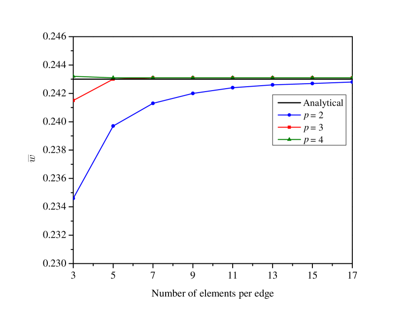
Figure 4: Convergence study of non-dimensional central deflection of homogeneous square microplates.

(a) Geometric configuration.

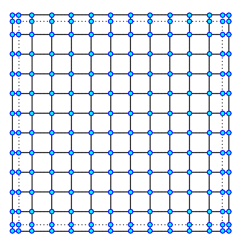
(b) Control point net and 11$\times$11 cubic elements.

Figure 5: Geometry and element mesh of a square microplate.

Further investigation on the accuracy of the proposed method is conducted using FG plates made of alumina and aluminum (Al/Al₂O₃). In this case, without considering couple stress effects, proposed RPT $(\varepsilon_{z}=0)$ and quasi-3D $(\varepsilon_{z}\neq 0)$ theories are applied in analysis of SSSS square plates using the rule of mixtures scheme. The plates are subjected to uniformly and sinusoidally distributed loads which are defined as $q_{0}$ and $q_{0}sin\left(\dfrac{\pi x}{a}\right)sin\left(\dfrac{\pi y}{a}\right)$, respectively. As can be observed in Table 4, the present results are in good agreement with those available in published works using various 2-D and quasi-3D theories. Apparently, these investigations have confirmed the validity and reliability of the present study.

Table 4: Comparison of non-dimensional deflection $\bar{w}=\dfrac{10E_{c}h^{3}}{q_{0}L^{4}}w\left(a/2,b/2,0\right)$ of SSSS Al/Al₂O₃ square plates (rule of mixtures scheme)

$n$	Theory	$\varepsilon_{z}=0$				$\varepsilon_{z}\neq 0$
		$a/h=4$	$a/h=10$	$a/h=100$		$a/h=4$	$a/h=10$	$a/h=100$
Sinusoidally distributed load
1	Zenkour [81]	-	-	-		0.6828	0.5592	0.5624
	Neves et al. [92]	-	-	-		0.6997	0.5845	0.5624
	Mantari and Soares [93]	-	-	-		0.693	0.569	0.545
	Carrera et al. [78]	0.7289	0.5890	0.5625		0.7171	0.5875	0.5625
	Akavci and Tanrikulu [94]	0.7282	0.5889	0.5625		0.6908	0.5691	0.5457
	Present†	0.7284	0.5889	0.5625		0.6935	0.5691	0.5460
4	Zenkour [81]	-	-	-		1.1001	0.8404	0.7933
	Neves et al. [92]	-	-	-		1.1178	0.8750	0.8286
	Mantari and Soares [93]	-	-	-		1.085	0.838	0.793
	Carrera et al. [78]	1.1673	0.8828	0.8286		1.1585	0.8821	0.8286
	Akavci and Tanrikulu [94]	1.1613	0.8818	0.8287		1.0983	0.8417	0.7925
	Present†	1.1590	0.8813	0.8287		1.0868	0.8392	0.7933
10	Zenkour [81]	-	-	-		1.3391	0.9806	0.9140
	Neves et al. [92]	-	-	-		1.3490	0.8750	0.8286
	Mantari and Soares [93]	-	-	-		1.308	0.972	0.911
	Carrera et al. [78]	1.3925	1.0090	0.9361		1.3745	1.0072	0.9361
	Akavci and Tanrikulu [94]	1.3917	1.0089	0.9362		1.3352	0.9818	0.9141
	Present†	1.3902	1.0086	0.9362		1.3116	0.9748	0.9132
Uniformly distributed load
1	Zenkour [7]	-	0.9287	-		-	-	-
	Akavci and Tanrikulu [94]	-	0.9288	-		-	0.8977	-
	Present†	1.1319	0.9288	0.8904		1.0788	0.8978	0.8642
4	Zenkour [7]	-	1.3890	-		-	-	-
	Akavci and Tanrikulu [94]	-	1.3888	-		-	1.3259	-
	Present†	1.7928	1.3882	1.3116		1.6827	1.3223	1.2556
10	Zenkour [7]	-	1.5876	-		-	-	-
	Akavci and Tanrikulu [94]	-	1.5875	-		-	1.5453	-
	Present†	2.1432	1.5870	1.4818		2.0244	1.5347	1.4454
†Proposed RPT and quasi-3D models are used for the case of $\varepsilon_{z}=0$ and $\varepsilon_{z}\neq 0$, respectively.

4.2 Static bending analysis

In this section, the static bending analysis of FG microplates based on modified couple stress theory will be investigated. The SSSS square microplates whose materials follow the rule of mixtures. The aspect ratio $a/h$, material length scale ratio $l/h$, and material index $n$ are taken into account. Table 5 presents the comparison of non-dimensional central deflection of SSSS square plate with those of Thai and Kim [43]. While the results generated from the proposed RPT theory are in very good agreement, quasi-3D theory yields slightly different responses in term of displacement. This is due to the consideration of the thickness stretching effect in the quasi-3D theory.

The bending responses of CCCC square Al/Al₂O₃ microplates under sinusoidally and uniformly distributed loads are further studied and presented in Table 6. It is noted that since there is no study on the static behaviours of CCCC microplates using MCST are reported in the literature, the results are compared with those generated from Reddy’s HSDT model [52] using the proposed IGA approach. As can be seen, the results based on Reddy’s model yields excellent agreement with proposed RPT-based solutions. The effects of material index $n$ and material length scale $l$ on the central displacement of CCCC square Al/Al₂O₃ plate are depicted in Fig. 6 in which data are generated by the proposed RPT and quasi-3D theories for three different ratios $l/h$ of 0, 0.4 and 1.0. As can be observed, the increase of material index $n$ leads to a rise of plates’ central deflection due to the decrease in plates’ stiffness. On the contrary, the growth of material length scale ratio $l/h$ is followed by a decline of displacement due to the increase in magnitude of stiffness matrix. In other word, for specific material length scale $l$, the thinner the microplates are, the higher plates’ stiffness would be. It can be further observed that the discrepancy in term of central deflection by the proposed RPT and quasi-3D is significantly decreased as $l/h$ increase and vanishes when $l/h=1.0$. Fig. 7 depicts the deformed configurations of the Al/Al₂O₃ square microplates with various boundary conditions subjected to sinusoidally distributed load in which $a/h,l/h$ and $n$ are equal to $5,0.4$ and $10$, respectively. It should be noted that the deformed shape of the microplates are scaled up for illustration purpose.

Table 5: Non-dimensional deflection $\bar{w}=\dfrac{10E_{c}h^{3}}{q_{0}L^{4}}w\left(a/2,b/2,0\right)$ of SSSS Al/Al₂O₃ square microplates subjected to sinusoidally distributed load (rule of mixtures scheme)

$a/h$	$l/h$	$n=0$				$n=1$				$n=10$
		RPT	Quasi-3D	TSDT[43]		RPT	Quasi-3D	TSDT[43]		RPT	Quasi-3D	TSDT[43]
5	0	0.3433	0.3360	0.3433		0.6688	0.6401	0.6688		1.2271	1.1663	1.2276
	0.2	0.2898	0.2853	0.2875		0.5505	0.5321	0.5468		1.0400	1.0019	1.0247
	0.4	0.1975	0.1965	0.1934		0.3601	0.3537	0.3535		0.7140	0.7043	0.6908
	0.6	0.1292	0.1296	0.1251		0.2288	0.2274	0.2224		0.4694	0.4711	0.4514
	0.8	0.0871	0.0879	0.0838		0.1517	0.1520	0.1464		0.3174	0.3220	0.3052
	1	0.0614	0.0623	0.0588		0.1060	0.1069	0.1017		0.2242	0.2289	0.2158
20	0	0.2842	0.2836	0.2842		0.5689	0.5516	0.5689		0.9537	0.9280	0.9538
	0.2	0.2431	0.2427	0.2430		0.4739	0.4619	0.4737		0.8313	0.8120	0.8303
	0.4	0.1695	0.1694	0.1693		0.3157	0.3105	0.3153		0.6001	0.5906	0.5986
	0.6	0.1127	0.1127	0.1124		0.2029	0.2008	0.2025		0.4102	0.4061	0.4090
	0.8	0.0767	0.0768	0.0765		0.1352	0.1343	0.1349		0.2842	0.2825	0.2834
	1	0.0544	0.0544	0.0542		0.0947	0.0943	0.0944		0.2038	0.2031	0.2033
100	0	0.2804	0.2803	0.2804		0.5625	0.5460	0.5625		0.9362	0.9132	0.9362
	0.2	0.2401	0.2400	0.2401		0.4689	0.4574	0.4689		0.8176	0.8001	0.8176
	0.4	0.1677	0.1677	0.1677		0.3128	0.3076	0.3128		0.5925	0.5833	0.5925
	0.6	0.1116	0.1116	0.1116		0.2012	0.1990	0.2011		0.4062	0.4018	0.4061
	0.8	0.0760	0.0760	0.0760		0.1341	0.1332	0.1341		0.2820	0.2799	0.2820
	1	0.0539	0.0539	0.0539		0.0939	0.0934	0.0939		0.2024	0.2014	0.2024

Table 6: Non-dimensional deflection $\bar{w}=\dfrac{10E_{c}h^{3}}{q_{0}L^{4}}w\left(a/2,b/2,0\right)$ of CCCC Al/Al₂O₃ square microplates (rule of mixtures scheme)

$a/h$	$l/h$	$n=0$				$n=1$				$n=10$
		RPT	Quasi-3D	IGA-Reddy		RPT	Quasi-3D	IGA-Reddy		RPT	Quasi-3D	IGA-Reddy
Sinusoidally distributed load
5	0	0.1601	0.1359	0.1601		0.3021	0.2554	0.3020		0.6111	0.4740	0.6113
	0.2	0.1378	0.1197	0.1377		0.2555	0.2214	0.2554		0.5178	0.4199	0.5183
	0.4	0.0974	0.0883	0.0973		0.1751	0.1586	0.1751		0.3568	0.3132	0.3575
	0.6	0.0655	0.0616	0.0655		0.1151	0.1081	0.1151		0.2358	0.2204	0.2364
	0.8	0.0450	0.0435	0.0449		0.0779	0.0752	0.0779		0.1602	0.1559	0.1606
	1	0.0321	0.0316	0.0320		0.0551	0.0542	0.0551		0.1136	0.1134	0.1139
20	0	0.1035	0.0950	0.1035		0.2065	0.1863	0.2065		0.3505	0.3150	0.3505
	0.2	0.0919	0.0849	0.0919		0.1797	0.1638	0.1797		0.3150	0.2857	0.3151
	0.4	0.0688	0.0645	0.0688		0.1294	0.1204	0.1294		0.2419	0.2237	0.2420
	0.6	0.0485	0.0462	0.0485		0.0882	0.0837	0.0882		0.1746	0.1647	0.1747
	0.8	0.0343	0.0331	0.0343		0.0611	0.0587	0.0611		0.1258	0.1204	0.1258
	1	0.0250	0.0243	0.0250		0.0438	0.0425	0.0438		0.0926	0.0896	0.0926
100	0	0.0999	0.0955	0.0999		0.2003	0.1872	0.2003		0.3336	0.3131	0.3336
	0.2	0.0889	0.0853	0.0889		0.1746	0.1643	0.1746		0.3013	0.2842	0.3013
	0.4	0.0668	0.0646	0.0668		0.1262	0.1204	0.1262		0.2336	0.2228	0.2336
	0.6	0.0473	0.0461	0.0473		0.0863	0.0835	0.0863		0.1701	0.1640	0.1701
	0.8	0.0336	0.0329	0.0336		0.0599	0.0584	0.0599		0.1232	0.1199	0.1233
	1	0.0244	0.0241	0.0244		0.0430	0.0422	0.0430		0.0910	0.0891	0.0910
Uniformly distributed load
5	0	0.2239	0.1860	0.2238		0.4220	0.3500	0.4219		0.8557	0.6408	0.8559
	0.2	0.1924	0.1641	0.1924		0.3566	0.3040	0.3565		0.7233	0.5701	0.7239
	0.4	0.1358	0.1215	0.1358		0.2443	0.2186	0.2442		0.4976	0.4286	0.4985
	0.6	0.0914	0.0851	0.0913		0.1606	0.1495	0.1605		0.3288	0.3034	0.3295
	0.8	0.0627	0.0602	0.0627		0.1087	0.1041	0.1087		0.2234	0.2154	0.2239
	1	0.0447	0.0439	0.0447		0.0769	0.0752	0.0769		0.1584	0.1570	0.1588
20	0	0.1436	0.1300	0.1436		0.2864	0.2553	0.2864		0.4863	0.4307	0.4863
	0.2	0.1275	0.1164	0.1275		0.2493	0.2248	0.2493		0.4372	0.3912	0.4373
	0.4	0.0956	0.0887	0.0956		0.1797	0.1657	0.1797		0.3360	0.3072	0.3361
	0.6	0.0674	0.0637	0.0674		0.1227	0.1156	0.1227		0.2428	0.2269	0.2429
	0.8	0.0478	0.0457	0.0478		0.0850	0.0813	0.0850		0.1750	0.1664	0.1751
	1	0.0348	0.0336	0.0348		0.0610	0.0589	0.0610		0.1289	0.1240	0.1289
100	0	0.1384	0.1314	0.1384		0.2775	0.2577	0.2775		0.4622	0.4310	0.4622
	0.2	0.1232	0.1174	0.1232		0.2421	0.2265	0.2421		0.4176	0.3915	0.4176
	0.4	0.0927	0.0891	0.0927		0.1751	0.1664	0.1751		0.3242	0.3075	0.3242
	0.6	0.0657	0.0637	0.0657		0.1199	0.1155	0.1199		0.2363	0.2268	0.2363
	0.8	0.0467	0.0456	0.0467		0.0833	0.0810	0.0833		0.1713	0.1661	0.1713
	1	0.0340	0.0334	0.0340		0.0598	0.0586	0.0598		0.1266	0.1236	0.1266]

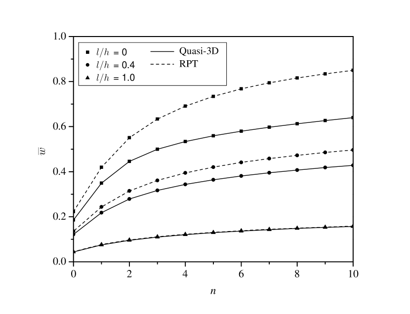
Figure 6: Effects of material index $n$ and material length scale ratio $l/h$ on the central deflection of CCCC Al/Al₂O₃ square microplates subjected to uniformly distributed load, $a/h=5$ (rule of mixtures scheme).

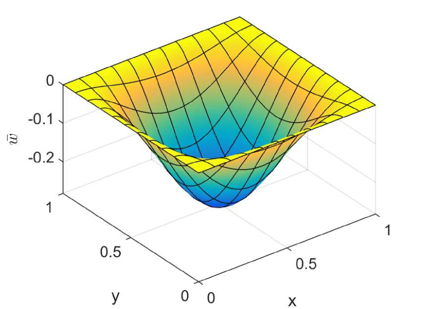
(a) CCCC.

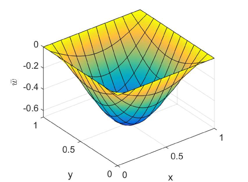
(b) SSSS.

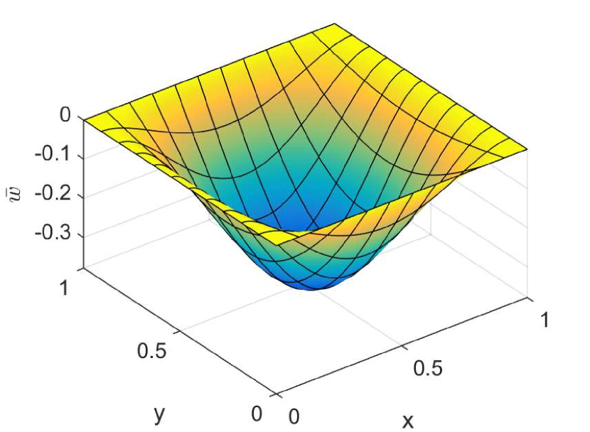
(c) SCSC.

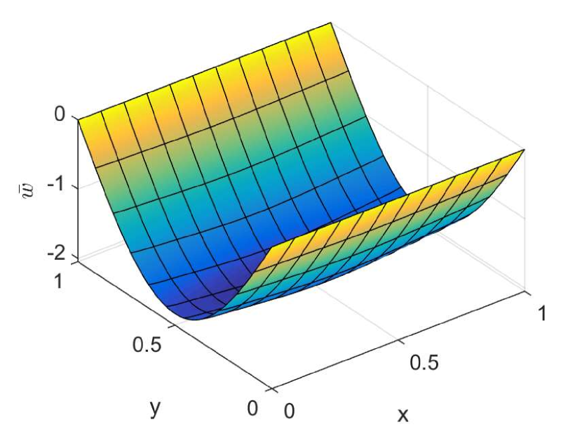
(d) SFSF.

Figure 7: Deformed configuration of Al/Al₂O₃ square microplates.

4.3 Free vibration analysis

In this part, the free vibration analysis of FG microplates based on modified couple stress theory will be discussed. The proposed Quasi-3D model is initially tested for normal-scale SSSS Al/ZrO₂-1 plates with various theories taking into account the normal shear deformation. It can be seen that the comparison results which are given in Table 7 agree well with those of other published works. The proposed RPT and quasi-3D models using IGA are further tested for homogeneous square microplates. The results which are shown in Table 8 are compared with analytical solutions generated from CPT by Yin et al. [35] and TSDT by Thai and Kim [43] . As can be observed, while the proposed RPT model yields slight discrepancy with respect to Yin et al.’s [35] due to their CPT assumption neglecting shear deformations, it shows excellent agreement with Thai and Kim’s [43], especially as plates become thinner, i.e. $a/h$ ratio is relatively large. Due to the consideration of thickness stretching effects, the proposed quasi-3D model gives slightly different results in comparison with other results.

Table 7: Comparison of non-dimensional natural frequencies $\bar{\omega}=\omega\dfrac{a^{2}}{h}\sqrt{\dfrac{\rho_{m}}{E_{m}}}$ of SSSS Al/ZrO₂-1 plates (Mori-Tanaka scheme)

Theory	$n=1$				$a/h=5$
	$a/h=5$	$a/h=10$	$a/h=20$		$n=2$	$n=3$	$n=5$
Vel and Batra [95]	5.4806	5.9609	6.1076		5.4923	5.5285	5.5632
Matsunaga [96]	5.7123	6.1932	6.3390		5.6599	5.6757	5.7020
Neves et al. [92]	5.4825	5.9600	6.1200		5.4950	5.5300	5.5625
Belabed et al. [97]	5.4800	5.9700	6.1200		5.5025	5.5350	5.5625
Alijani and Amabili [98]	5.4796	5.9578	6.1040		5.4919	5.5279	5.5633
Akavci and Tanrikulu [94]	5.4829	5.9676	6.1160		5.5064	5.5388	5.5644
Present	5.5172	6.0023	6.1505		5.5324	5.5642	5.5886

Table 8: Comparison of non-dimensional natural frequencies $\bar{\omega}=\omega\dfrac{a^{2}}{h}\sqrt{\dfrac{\rho}{E}}$ of SSSS homogeneous microplates

$a/h$	Theory	$l/h$
		0	0.2	0.4	0.6	0.8	1
5	CPT [35]	5.9734	6.4556	7.7239	9.4673	11.4713	13.6213
	TSDT [43]	5.2813	5.7699	7.0330	8.7389	10.6766	12.7408
	RPT (Present)	5.2813	5.7496	6.9667	8.6191	9.8943	9.9791
	Quasi-3D (Present)	5.3090	5.7622	6.9438	8.5509	9.8943	9.9791
20	CPT [35]	5.9734	6.4556	7.7239	9.4673	11.4713	13.6213
	TSDT [43]	5.9199	6.4027	7.6708	9.4116	11.4108	13.5545
	RPT (Present)	5.9199	6.4009	7.6646	9.4005	11.3945	13.5330
	Quasi-3D (Present)	5.9235	6.4030	7.6633	9.3952	11.3854	13.5202
100	CPT [35]	5.9734	6.4556	7.7239	9.4673	11.4713	13.6213
	TSDT [43]	5.9712	6.4535	7.7217	9.4651	11.4689	13.6186
	RPT (Present)	5.9712	6.4534	7.7215	9.4646	11.4682	13.6178
	Quasi-3D (Present)	5.9723	6.4544	7.7222	9.4650	11.4683	13.6177

Table 9 presents non-dimensional natural frequency of SSSS Al/Al₂O₃ square microplates. The results are compared with those of Thai and Kim [43] in which analytical approach based on TSDT model is employed. Thick $(a/h=5)$, moderately thick $(a/h=20)$ and thin $(a/h=100)$ microplates are considered. The results reveal good agreement between RPT model and TSDT [43], especially when the material length scale ratio $l/h$ is small, e.g. 0 or 0.2. On the contrary, the discrepancy becomes larger as $l/h$ gets closer to 1. However, this phenomenon just happens for thick plates and tends to be vague as the plates become thinner. Meanwhile, the quasi-3D gives slightly different results compared to that of RPT model. General observation from Table 9 reveals that the higher material length scale ratio is chosen, the bigger natural frequencies of the plates could be obtained as a result of the increase in plate’s stiffness. Fig. 8 provides a closer look at the effects of material index $n$ and material length scale $l$ on the plates’ natural frequencies which are computed using proposed RPT and quasi-3D models. Similar to the previous case of bending analysis, the plate’s stiffness decreases as a result of rising in material index $n$ and falling in material length scale ratio $l/h$ which leads to the decrease of natural frequency of the plates. In addition, the discrepancy in term of frequency results predicted by the proposed RPT and quasi-3D becomes less significant as $l/h$ gets bigger and is almost zero difference when $l/h=1.0$. The first six natural frequencies of Al/Al₂O₃ square microplates with different types of boundary conditions are given in Table 10 in which the results are generated for $n=1$ and $l/h=0.2$. The present quasi-3D results show good agreement with those of Zenkour’s quasi-3D model [81] using the proposed IGA approach. The first six mode shapes corresponding to the quasi-3D vibration analysis of CCCC microplates with $a/h=10$ are presented in Fig. 9.

Table 9: Non-dimensional natural frequency $\bar{\omega}=\omega\dfrac{a^{2}}{h}\sqrt{\dfrac{\rho_{c}}{E_{c}}}$ of SSSS Al/Al₂O₃ square plates (rule of mixtures scheme)

$a/h$	$l/h$	$n=0$				$n=1$				$n=10$
		RPT	Quasi-3D	TSDT[43]		RPT	Quasi-3D	TSDT[43]		RPT	Quasi-3D	TSDT[43]
5	0	5.2813	5.3090	5.2813		4.0781	4.1521	4.0781		3.2519	3.3126	3.2514
	0.2	5.7496	5.7622	5.7699		4.4959	4.5542	4.5094		3.5312	3.5740	3.5548
	0.4	6.9667	6.9438	7.0330		5.5620	5.5865	5.6071		4.2584	4.2627	4.3200
	0.6	8.6191	8.5509	8.7389		6.9822	6.9681	7.0662		5.2471	5.2115	5.3335
	0.8	9.8943	9.8943	10.6766		8.2313	8.2313	8.7058		5.8571	5.8571	6.4759
	1	9.9791	9.9791	12.7408		8.3019	8.3019	10.4397		5.9073	5.9073	7.6895
20	0	5.9199	5.9235	5.9199		4.5228	4.5919	4.5228		3.7623	3.8129	3.7622
	0.2	6.4009	6.4030	6.4027		4.9556	5.0179	4.9568		4.0299	4.0761	4.0323
	0.4	7.6646	7.6633	7.6708		6.0714	6.1203	6.0756		4.7428	4.7794	4.7488
	0.6	9.4005	9.3952	9.4116		7.5739	7.6107	7.5817		5.7369	5.7640	5.7453
	0.8	11.3945	11.3854	11.4108		9.2768	9.3042	9.2887		6.8914	6.9106	6.9013
	1	13.5330	13.5202	13.5545		11.0882	11.1082	11.1042		8.1384	8.1510	8.1494
100	0	5.9712	5.9723	5.9712		4.5579	4.6263	4.5579		3.8058	3.8533	3.8058
	0.2	6.4534	6.4544	6.4535		4.9922	5.0546	4.9922		4.0724	4.1168	4.0725
	0.4	7.7215	7.7222	7.7217		6.1124	6.1635	6.1126		4.7837	4.8215	4.7840
	0.6	9.4646	9.4650	9.4651		7.6220	7.6630	7.6224		5.7778	5.8090	5.7782
	0.8	11.4682	11.4683	11.4689		9.3339	9.3673	9.3344		6.9341	6.9600	6.9345
	1	13.6178	13.6177	13.6186		11.1554	11.1832	11.1560		8.1842	8.2060	8.1846

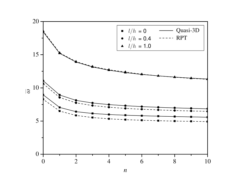
Figure 8: Effects of material index $n$ and material length scale ratio $l/h$ on the natural frequency of CCCC Al/Al₂O₃ square microplates, $a/h=5$ (rule of mixtures scheme).

Table 10: The first six non-dimensional natural frequencies $\bar{\omega}=\omega\dfrac{a^{2}}{h}\sqrt{\dfrac{\rho_{m}}{E_{m}}}$ of Al/Al₂O₃ square plates (Mori-Tanaka scheme)

BC	$a/h$	Theory	Mode
			1	2	3	4	5	6
SSSS	5	IGA-Zenkour	7.9366	13.8049	13.8049	17.3259	17.3259	19.5422
		Quasi-3D (Present)	7.8883	13.8049	13.8049	17.2045	17.2045	19.5422
		RPT (Present)	7.7844	13.8049	13.8049	16.9943	16.9943	19.5422
	10	IGA-Zenkour	8.5940	20.3230	20.3230	27.5893	27.5893	31.7475
		Quasi-3D (Present)	8.5607	20.2031	20.2031	27.5893	27.5893	31.5547
		RPT (Present)	8.4401	19.9188	19.9188	27.5893	27.5893	31.1386
	100	IGA-Zenkour	8.8399	21.7851	21.7851	35.3333	43.0764	43.0764
		Quasi-3D (Present)	8.8390	21.7802	21.7802	35.3221	43.0573	43.0573
		RPT (Present)	8.7127	21.4598	21.4598	34.8171	42.4074	42.4074
CCCC	5	IGA-Zenkour	12.7213	22.6661	22.6661	27.9021	27.9021	31.1450
		Quasi-3D (Present)	13.1029	22.9300	22.9300	27.8791	27.8791	31.3005
		RPT (Present)	12.1531	22.0683	22.0683	26.3182	26.3182	30.5398
	10	IGA-Zenkour	15.2379	28.9665	28.9665	41.2221	47.8649	47.9221
		Quasi-3D (Present)	15.4413	29.3267	29.3267	41.5955	48.2657	48.4504
		RPT (Present)	14.3638	27.8276	27.8276	39.9305	46.0435	46.4772
	100	IGA-Zenkour	16.0795	32.6473	32.6473	48.5912	58.0858	58.3951
		Quasi-3D (Present)	16.0540	32.6082	32.6082	48.5477	58.0353	58.3402
		RPT (Present)	15.5212	31.5708	31.5708	47.0903	56.2566	56.5207

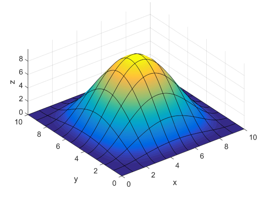
(a) $\bar{\omega}_{1}=15.4413$.

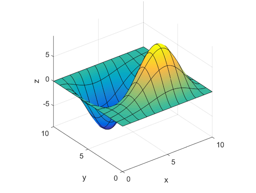
(b) $\bar{\omega}_{2}=29.3267$.

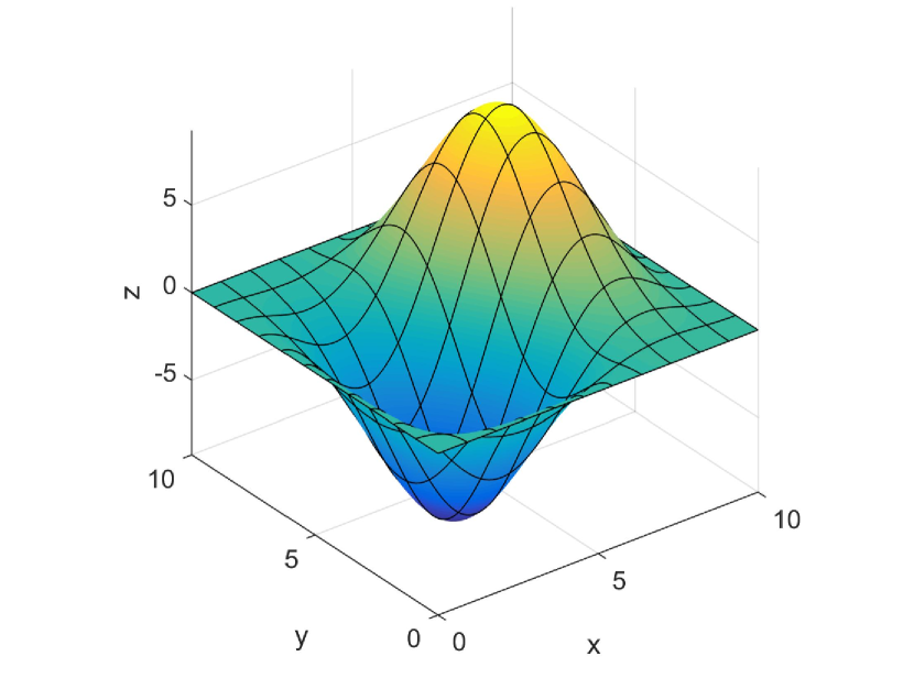
(c) $\bar{\omega}_{3}=29.3267$.

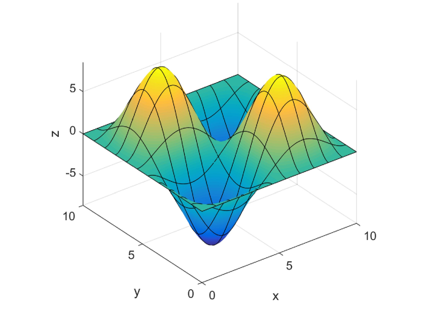
(d) $\bar{\omega}_{4}=41.5955$.

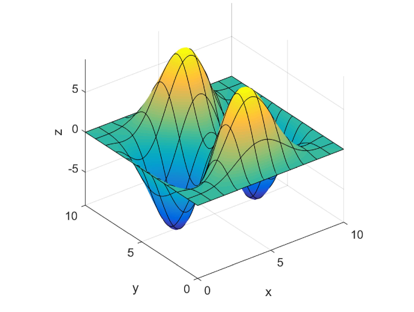
(e) $\bar{\omega}_{5}=48.2657$.

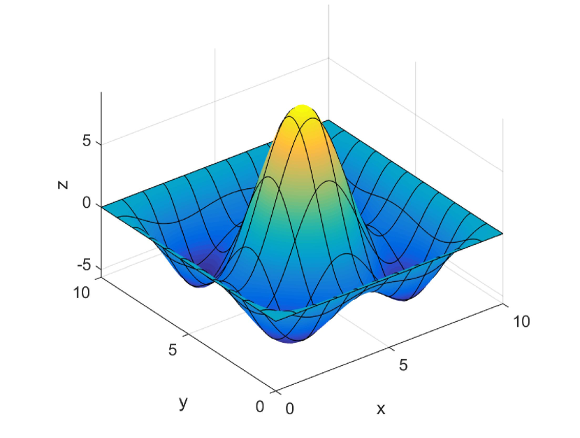
(f) $\bar{\omega}_{6}=48.4504$.

Figure 9: The first six free vibration mode shapes of Al/Al₂O₃ CCCC square microplates.

Next, free vibration of circular plates whose geometry configuration and mesh are shown in Fig. 10 will be investigated. Since there is no publication on the vibration behaviours of FG circular microplates based on the modified couple stress theory is found, the investigation of circulars could be served as benchmark examples. Table 11 presents the fundamental natural frequencies which are firstly tested for homogeneous plates. Natural frequencies of plates without considering size-dependent effects $(l=0)$ are compared with results reported by Mohammandi et al. [88] and Nguyen et al. [85]. The results show very good agreement between the theories, especially proposed RPT and Nguyen et al.’s [85] which also uses another polynomial-based RPT model. Table 12 presents the first six natural frequencies of Al/Al₂O₃ circular plates with simple and clamped supports. The plates’ thickness $h$ and material index $n$ are set as $0.2R$ and 1, respectively. As previous case of square microplates, Zenkour’s quasi-3D model [81] using proposed IGA approach is added for reference purpose since there is no study can be found for this analysis problem. The six fundamental mode shapes of clamped plates with $l/h=0.2$ using quasi-3D model are printed in Fig. 11.

(a) Geometric configuration.

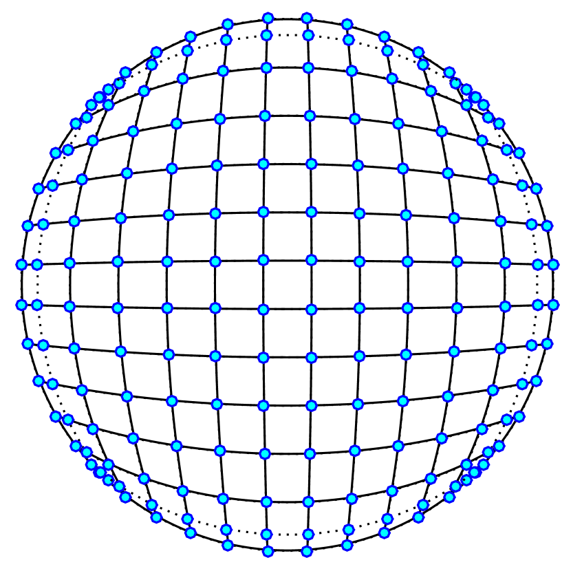
(b) Control point net and 11$\times$11 cubic elements.

Figure 10: Geometry and element mesh of a circular microplate.

Table 11: The first six non-dimensional natural frequencies $\bar{\omega}=\omega R^{2}\sqrt{\dfrac{\rho h}{D^{\dagger}}}$ of homogeneous circular microplates

$l/h$	Theory	Mode
		1	2	3	4	5	6
Simple support
0	Mohammadi et al. [88]	4.9345	13.8981	25.6132	29.7198	39.9571	48.4788
	Nguyen et al. [85]	4.9304	13.8587	25.4798	29.5390	39.6331	48.0046
	RPT (Present)	4.9304	13.8591	25.4799	29.5456	39.6518	48.0402
	Quasi-3D (Present)	4.9385	13.8701	25.4983	29.5691	39.6881	48.0906
0.2	RPT (Present)	4.9925	14.5095	26.5426	31.1786	41.8855	50.8427
	Quasi-3D (Present)	5.0024	14.5206	26.5613	31.1981	41.9148	50.8808
0.4	RPT (Present)	5.1213	16.2743	29.4369	35.5996	47.7406	58.5547
	Quasi-3D (Present)	5.1365	16.2857	29.4529	35.6092	47.7542	58.5621
0.6	RPT (Present)	5.2422	18.8078	33.6370	41.9096	55.8684	69.6631
	Quasi-3D (Present)	5.2649	18.8192	33.6497	41.9065	55.8623	69.6331
0.8	RPT (Present)	5.3324	21.8342	38.6993	49.3881	65.3972	82.8177
	Quasi-3D (Present)	5.3642	21.8450	38.7080	49.3713	65.3694	82.7497
1	RPT (Present)	5.3954	25.1769	44.3292	57.5842	75.8223	97.1772
	Quasi-3D (Present)	5.4379	25.1869	44.3335	57.5538	75.7721	97.0720
Clamped support
0	Mohammadi et al. [88]	10.2158	21.2604	34.8772	39.7706	51.0295	60.8290
	Nguyen et al. [85]	10.1839	21.1433	34.5892	39.3624	50.4385	59.9580
	RPT (Present)	10.1842	21.1459	34.5885	39.3832	50.4865	60.0416
	Quasi-3D (Present)	10.4466	21.6458	35.2774	40.2833	51.5045	61.3186
0.2	RPT (Present)	10.8087	22.4449	36.3961	41.8103	53.5802	63.7743
	Quasi-3D (Present)	11.0612	22.9236	37.1800	42.6664	54.5550	64.9738
0.4	RPT (Present)	12.4963	25.9527	41.2953	48.3406	61.7419	73.9729
	Quasi-3D (Present)	12.7255	26.3811	41.9956	49.0934	62.6149	74.9922
0.6	RPT (Present)	14.8897	30.9242	48.3696	57.5674	73.1139	88.5334
	Quasi-3D (Present)	15.0927	31.2968	48.9732	58.2073	73.8637	89.3634
0.8	RPT (Present)	17.7051	36.7699	56.8123	68.4011	86.4224	105.6689
	Quasi-3D (Present)	17.8850	37.0938	57.3265	68.9439	87.0506	106.3411
1	RPT (Present)	20.7715	43.1360	66.1009	80.1939	100.9243	124.3039
	Quasi-3D (Present)	20.9330	43.4206	66.5388	80.6591	101.4425	124.8498
${}^{\dagger}D=\dfrac{Eh^{3}}{12(1-\nu^{2})}$

Table 12: The first six non-dimensional natural frequencies $\bar{\omega}=\omega R^{2}\sqrt{\dfrac{\rho_{c}h}{D_{c}^{\dagger}}}$ of Al/Al₂O₃ circular microplates (Mori-Tanaka scheme)

$l/h$	Theory	Mode
		1	2	3	4	5	6
Simple support
0	IGA-Zenkour	3.4629	8.9254	8.9254	12.9890	12.9890	15.4780
	Quasi-3D (Present)	3.4132	8.8258	8.8258	12.9916	12.9916	15.3331
	RPT (Present)	3.3572	8.6722	8.6722	12.9121	12.9121	15.0490
0.2	IGA-Zenkour	3.5224	9.3961	9.3961	13.1894	13.1894	16.2612
	Quasi-3D (Present)	3.4675	9.2928	9.2928	13.1928	13.1928	16.1022
	RPT (Present)	3.4118	9.1595	9.1595	13.1037	13.1037	15.8706
0.4	IGA-Zenkour	3.6392	10.6411	10.6411	13.3115	13.3115	18.2644
	Quasi-3D (Present)	3.5698	10.5288	10.5288	13.3143	13.3143	18.1203
	RPT (Present)	3.5114	10.4415	10.4415	13.2326	13.2326	18.0361
0.6	IGA-Zenkour	3.7577	12.2959	12.2959	13.5601	13.5601	18.4956
	Quasi-3D (Present)	3.6687	12.1873	12.1873	13.5445	13.5445	18.4939
	RPT (Present)	3.6018	12.1378	12.1378	13.4872	13.4872	18.4475
0.8	IGA-Zenkour	3.8632	13.2220	13.2220	14.8766	14.8766	18.6662
	Quasi-3D (Present)	3.7546	13.2030	13.2030	14.7552	14.7552	18.6655
	RPT (Present)	3.6721	13.1245	13.1245	14.7850	14.7850	18.6192
1	IGA-Zenkour	3.9548	13.4288	13.4288	17.1268	17.1268	18.8623
	Quasi-3D (Present)	3.8303	13.4243	13.4243	16.9751	16.9751	18.8618
	RPT (Present)	3.9557	13.5531	13.5531	17.4735	17.4735	18.8633
Clamped support
0	IGA-Zenkour	6.7718	12.9968	12.9968	19.8267	19.8608	21.9673
	Quasi-3D (Present)	6.8745	13.1770	13.1770	20.0202	20.0388	22.2840
	RPT (Present)	6.3384	12.4133	12.4133	19.0879	19.1363	20.9877
0.2	IGA-Zenkour	7.2163	13.9289	13.9289	21.1653	21.5889	23.7182
	Quasi-3D (Present)	7.3195	14.0950	14.0950	21.3095	21.7503	23.9885
	RPT (Present)	6.8208	13.4172	13.4172	20.5401	20.9799	22.8902
0.4	IGA-Zenkour	8.4091	16.4035	16.4035	24.6620	25.9011	25.9011
	Quasi-3D (Present)	8.5121	16.5390	16.5390	24.7273	25.8504	25.8504
	RPT (Present)	8.0909	16.0391	16.0391	24.2526	24.3345	24.3345
0.6	IGA-Zenkour	10.0860	19.8463	19.8463	25.9424	25.9424	28.6525
	Quasi-3D (Present)	10.1880	19.9431	19.9431	25.8948	25.8948	28.6525
	RPT (Present)	9.8463	19.6321	19.6321	24.3655	24.3655	28.6525
0.8	IGA-Zenkour	12.0447	23.8379	23.8379	25.9920	25.9920	28.9380
	Quasi-3D (Present)	12.1441	23.8850	23.8850	25.9507	25.9507	28.9380
	RPT (Present)	11.8741	23.7016	23.7016	24.4627	24.4627	28.9380
1	IGA-Zenkour	14.1674	26.0476	26.0476	28.1435	28.1435	29.3010
	Quasi-3D (Present)	14.2615	25.9953	25.9953	28.1492	28.1492	29.3010
	RPT (Present)	14.0568	24.4150	24.4150	28.2217	28.2217	29.3010
${}^{\dagger}D_{c}=\dfrac{E_{c}h^{3}}{12(1-\nu_{c}^{2})}$

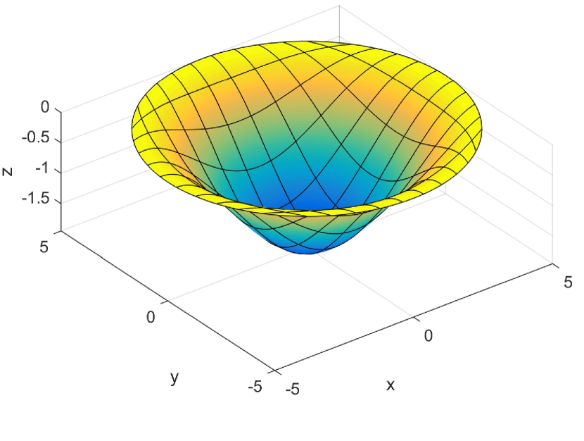
(a) $\bar{\omega}_{1}=7.3195$.

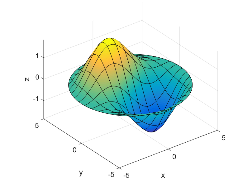
(b) $\bar{\omega}_{2}=14.0950$.

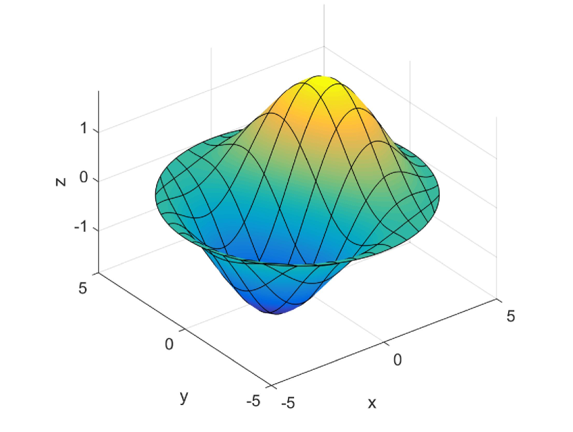
(c) $\bar{\omega}_{3}=14.0950$.

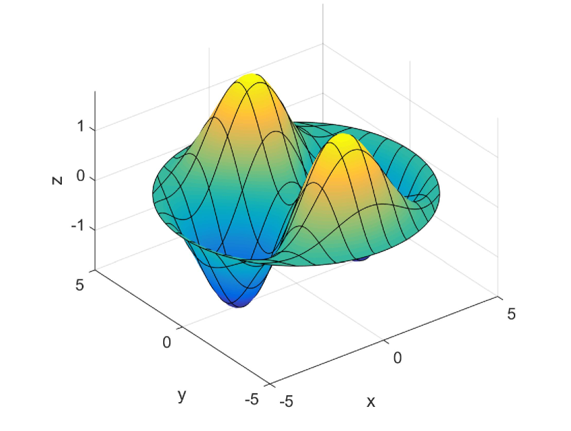
(d) $\bar{\omega}_{4}=21.3095$.

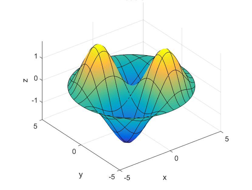
(e) $\bar{\omega}_{5}=21.7503$.

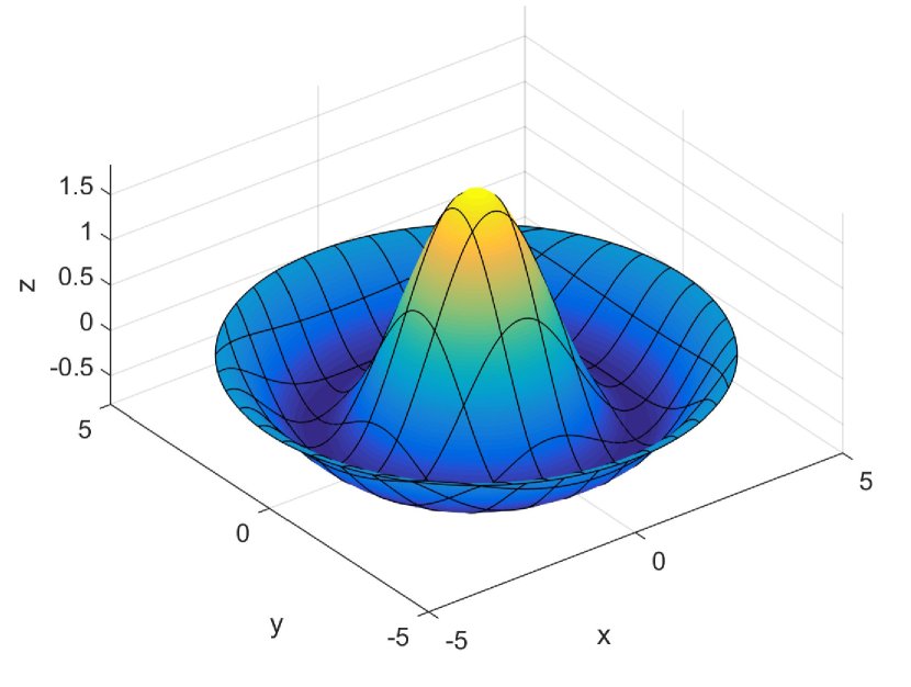
(f) $\bar{\omega}_{6}=23.9885$.

Figure 11: The first six free vibration mode shapes of clamped Al/Al₂O₃ circular microplates.

4.4 Buckling analysis

In this stage, buckling behaviours of square and circular FG microplates will be discussed. In order to verify the proposed method and models in dealing with buckling analysis, first attempt is to calculate the critical buckling load of SSSS FG microplates bearing biaxial load. The results are compared with analytical solutions based on CPT and FSDT by Thai and Choi [44] and RPT by He et al. [48] for which material properties are $E_{1}=14.4$GPa, $\rho_{1}=12.2\times 10^{3}$kg/m³, $E_{2}=1.44$GPa, $\rho_{2}=1.22\times 10^{3}$kg/m³, $\nu_{1}=\nu_{2}=0.38$. As can be seen in Table 13, although there is discrepancy for the case of thick microplates $(a/h=5)$, the results predicted by proposed RPT theory are in good agreement with those calculated by FSDT [44] and RPT [48] as plates become thinner. On the other hand, while CPT-based solutions are of remarkable difference to that of FDST and RPTs due to the ignorance of shear deformations, especially for thick plates, the proposed quasi-3D theory which takes into account normal deformation yields similar results with respect to those of shear deformable theories of FSDT and RPTs.

Table 13: Comparison of non-dimensional critical buckling load $\bar{P}_{cr}=\dfrac{P_{cr}a^{2}}{E_{2}h^{3}}$ of square FG microplates (rule of mixtures scheme)

$l/h$	Theory	$a/h=5$				$a/h=10$				$a/h=20$
		$n=0$	$n=1$	$n=10$		$n=0$	$n=1$	$n=10$		$n=0$	$n=1$	$n=10$
0	CPT [44]	19.2255	8.2145	3.8359		19.2255	8.2145	3.8359		19.2255	8.2145	3.8359
	FSDT [44]	15.3228	6.8576	2.9979		18.0746	7.8273	3.5853		18.9243	8.1142	3.7700
	RPT [48]	15.3322	6.8611	2.7672		18.0754	7.8276	3.4969		18.9243	8.1142	3.7450
	RPT†	15.3321	6.8610	2.7702		18.0756	7.8277	3.4982		18.9244	8.1143	3.7454
	Quasi-3D†	15.3629	7.3905	3.0118		18.1561	8.5396	3.8921		18.9675	8.8639	4.1850
0.2	CPT [44]	22.0863	9.7879	4.3560		22.0863	9.7879	4.3560		22.0863	9.7879	4.3560
	FSDT [44]	17.6150	8.1715	3.4076		20.7607	9.3241	4.0710		21.7387	9.6675	4.2809
	RPT [48]	18.0422	8.3399	3.3619		20.9025	9.3767	4.0513		21.7771	9.6815	4.2752
	RPT†	17.8878	8.2820	3.2917		20.8497	9.3581	4.0246		21.7628	9.6766	4.2677
	Quasi-3D†	17.7286	8.7153	3.4728		20.8583	10.0344	4.3958		21.7852	10.4160	4.7009
0.4	CPT [44]	30.6685	14.5082	5.9164		30.6685	14.5082	5.9164		30.6685	14.5082	5.9164
	FSDT [44]	24.2899	11.9922	4.6013		28.7478	13.7742	5.5151		30.1625	14.3167	5.8102
	RPT [48]	26.1539	12.7754	5.0407		29.3735	14.0232	5.6631		30.3324	14.3832	5.8505
	RPT†	25.5457	12.5322	4.8371		29.1700	13.9459	5.5925		30.2773	14.3626	5.8312
	Quasi-3D†	24.8060	12.6741	4.8557		28.9624	14.5168	5.9066		30.2381	15.0722	6.2486
0.6	CPT [44]	44.9723	22.3753	8.5171		44.9723	22.3753	8.5171		44.9723	22.3753	8.5171
	FSDT [44]	34.7856	17.9838	6.4804		41.8271	21.0597	7.8802		44.1369	22.0292	8.3472
	RPT [48]	39.6393	20.1658	7.7001		43.4732	21.7657	8.2906		44.5855	22.2188	8.4589
	RPT†	38.2867	19.5858	7.3772		43.0329	21.5846	8.1871		44.4673	22.1708	8.4312
	Quasi-3D†	36.5415	19.2256	7.1597		42.4620	21.9814	8.4246		44.3258	22.8320	8.8281
0.8	CPT [44]	64.9976	33.3892	12.1581		64.9976	33.3892	12.1581		64.9976	33.3892	12.1581
	FSDT [44]	48.2915	25.6654	8.9020		59.6657	30.9928	11.1065		63.5656	32.7517	11.8745
	RPT [48]	58.4862	30.5105	11.3322		63.1958	32.6036	11.9349		64.5348	33.1882	12.1011
	RPT†	56.0961	29.4240	10.9005		62.4358	32.2693	11.8036		64.3321	33.0999	12.0666
	Quasi-3D†	52.8623	28.3151	10.3843		61.3467	32.4199	11.9498		64.0474	33.6948	12.4394
1	CPT [44]	90.7444	47.5499	16.8393		90.7444	47.5499	16.8393		-	-	-
	FSDT [44]	63.8913	34.4981	11.7042		81.8269	43.3274	15.1152		-	-	-
	RPT [48]	82.6938	43.8094	15.9522		88.5416	46.5372	16.6033		90.1804	47.2914	16.7793
	RPT†	78.9675	42.0388	15.4071		87.3775	45.9981	16.4431		89.8715	47.1494	16.7376
	Quasi-3D†	73.6925	39.8872	14.5287		85.6043	45.8223	16.4819		89.4018	47.6596	17.0825
†Present

Table 14 presents the biaxial buckling analysis results of Al/Al₂O₃ square microplates. The results are calculated based on the proposed RPT and quasi-3D theories which could be served as benchmark examples for future references since no report in the similar case is found. The first six non-dimensional biaxial buckling loads of Al/Al₂O₃ square plates are reported in Table 15 for $n=10$ and $l/h=0.2$. While the results generated from the proposed quasi-3D and IGA-based Zenkour’s quasi-3D theories [81] are relatively close to each other for both type of boundary conditions, the RPT’s show remarkable discrepancy to the other theories, especially for the CCCC plates. This is due to the consideration of normal deformation of the quasi-3D theories. For $a/h=5$, six buckling mode shapes of CCCC plates based on the proposed quasi-3D theory which are scaled up for illustration purposes are presented in Fig. 12.

Table 14: Non-dimensional critical buckling load $\bar{P}_{cr}=\dfrac{P_{cr}a^{2}}{D_{m}^{\dagger}}$ of Al/Al₂O₃ square microplates (Mori-Tanaka scheme)

BC	$a/h$	$l/h$	$n=0$			$n=1$			$n=10$
			RPT	Quasi-3D		RPT	Quasi-3D		RPT	Quasi-3D
SSSS	5	0	87.4747	86.5475		35.0795	35.6610		21.7236	21.7189
		0.2	103.6359	101.8797		42.3816	42.6185		25.4909	25.2307
		0.4	152.0215	147.6312		64.2668	63.3902		36.7873	35.7417
		0.6	232.4351	223.1633		100.6957	97.7189		55.6034	53.1891
		0.8	344.7280	327.6683		151.6424	145.2904		81.9336	77.4961
		1	488.8378	460.3907		217.0988	205.8260		115.7764	108.5941
	20	0	105.6668	105.6221		42.0033	43.4065		27.5182	27.8578
		0.2	123.5339	123.4102		49.9504	51.3272		31.5521	31.8705
		0.4	177.1295	176.7715		73.7907	75.0881		43.6520	43.9085
		0.6	266.4425	265.6972		113.5226	114.6856		63.8152	63.9707
		0.8	391.4648	390.1733		169.1451	170.1141		92.0401	92.0558
		1	552.1931	550.1813		240.6580	241.3659		128.3267	128.1618
	100	0	107.0958	107.1271		42.5423	44.0165		27.9978	28.3566
		0.2	125.0926	125.1206		50.5370	52.0102		32.0486	32.4065
		0.4	179.0825	179.1009		74.5212	75.9913		44.2009	44.5563
		0.6	269.0653	269.0682		114.4947	115.9596		64.4546	64.8061
		0.8	395.0406	395.0223		170.4576	171.9154		92.8097	93.1557
		1	557.0082	556.9633		242.4098	243.8584		129.2661	129.6052
CCCC	5	0	178.2578	188.3478		72.2150	78.0421		42.1220	45.4860
		0.2	206.9297	215.7331		85.4028	90.6731		49.1101	52.1032
		0.4	292.6287	295.5433		124.8630	127.4320		69.9984	71.1001
		0.6	435.0030	424.8837		190.5274	187.0650		104.7011	101.8084
		0.8	633.8611	601.6084		282.3839	268.7548		153.1709	144.0664
		1	889.1171	823.8983		400.4310	371.8457		215.3906	197.7752
	20	0	273.9507	288.6976		109.0237	117.3906		70.8926	75.2177
		0.2	308.7803	323.9291		124.5481	133.0578		78.8262	83.2085
		0.4	413.0833	429.0109		171.0330	179.8054		102.5575	107.0378
		0.6	586.6304	603.0356		248.3764	257.2793		141.9833	146.4815
		0.8	829.3607	845.5938		356.5558	365.3387		197.0586	201.4295
		1	1141.2885	1156.5929		495.5793	503.9582		267.7793	271.8584
	100	0	283.7646	292.2008		112.7294	119.3117		74.1644	77.0743
		0.2	319.1326	327.9091		128.4414	135.1344		82.1289	85.1055
		0.4	425.0550	434.6081		175.4917	182.4322		105.9838	109.1182
		0.6	601.2918	611.6685		253.7742	260.9696		145.6726	148.9836
		0.8	847.7694	858.8291		363.2623	370.6627		201.1735	204.6383
		1	1164.4998	1176.0787		503.9643	511.5167		272.4865	276.0730
${}^{\dagger}D_{m}=\dfrac{E_{m}h^{3}}{12(1-\nu_{m}^{2})}$

Table 15: The first six non-dimensional buckling loads $\bar{P}=\dfrac{Pa^{2}}{D_{m}}$ of Al/Al₂O₃ square microplates, $n=10$, $l/h=0.2$ (Mori-Tanaka scheme)

BC	$a/h$	Theory	Mode
			1	2	3	4	5	6
SSSS	5	IGA-Zenkour	25.4064	47.0158	47.0158	62.7947	66.4706	66.4706
		Quasi-3D (Present)	25.2307	46.2828	46.2828	61.4689	64.8256	64.8256
		RPT (Present)	25.4909	47.9306	47.9306	64.7895	68.7456	68.7456
	10	IGA-Zenkour	30.3554	67.5835	67.5835	101.6321	115.5866	115.5866
		Quasi-3D (Present)	30.2890	67.2254	67.2254	100.9300	114.4706	114.4706
		RPT (Present)	30.1012	67.3570	67.3570	101.9693	116.1512	116.1512
	20	IGA-Zenkour	31.8815	76.0319	76.0319	121.4313	143.5095	143.5095
		Quasi-3D (Present)	31.8705	75.8988	75.8988	121.1662	143.0021	143.0021
		RPT (Present)	31.5521	75.2628	75.2628	120.4131	142.2468	142.2468
	100	IGA-Zenkour	32.3844	79.0722	79.0722	129.2976	155.1773	155.1773
		Quasi-3D (Present)	32.4065	79.1198	79.1198	129.3662	155.2457	155.2457
		RPT (Present)	32.0486	78.2296	78.2296	127.9519	153.4678	153.4678
CCCC	5	IGA-Zenkour	50.6557	66.0350	66.0350	78.0114	80.2597	84.0819
		Quasi-3D (Present)	52.1032	66.3156	66.3156	77.2179	78.9774	84.1043
		RPT (Present)	49.1101	66.7907	66.7907	80.3088	82.9464	85.5400
	10	IGA-Zenkour	74.8665	114.2196	114.2196	146.4170	160.1781	172.6816
		Quasi-3D (Present)	75.4661	115.7598	115.7598	147.8696	161.3725	174.2442
		RPT (Present)	70.1001	110.6293	110.6293	144.4919	158.8413	167.4729
	20	IGA-Zenkour	83.8952	140.5084	140.5084	191.9601	219.4306	239.0973
		Quasi-3D (Present)	83.2085	140.4610	140.4610	192.6237	220.3776	239.1104
		RPT (Present)	78.8262	133.9531	133.9531	185.0964	211.8925	227.4324
	100	IGA-Zenkour	85.2475	149.0723	149.0723	210.8794	246.4373	267.8293
		Quasi-3D (Present)	85.1055	148.8861	148.8861	210.7133	246.2408	267.4391
		RPT (Present)	82.1289	143.8128	143.8128	203.9109	237.9639	257.7571

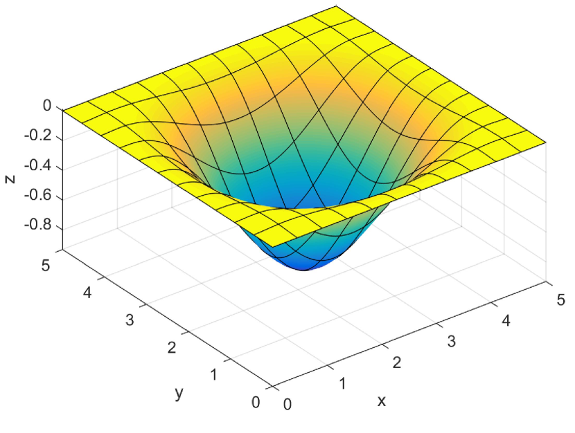
(a) $\bar{P}_{1}=52.1032$.

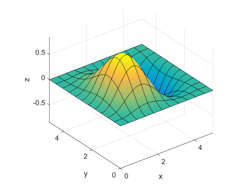
(b) $\bar{P}_{2}=66.3156$.

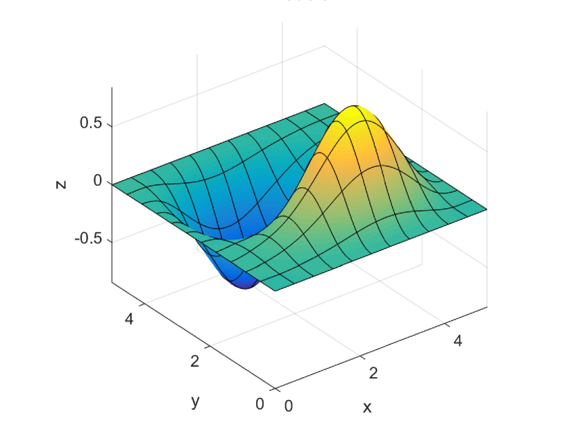
(c) $\bar{P}_{3}=66.3156$.

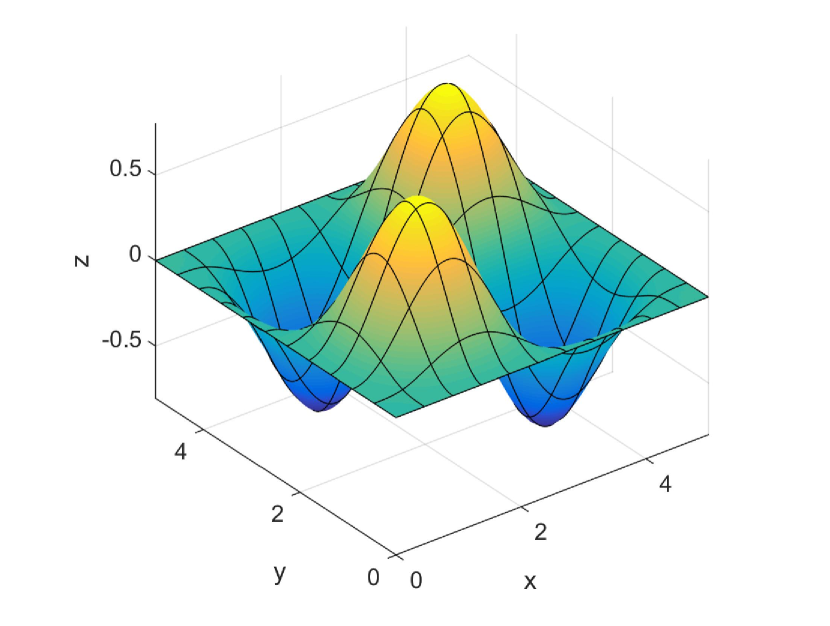
(d) $\bar{P}_{4}=77.2179$.

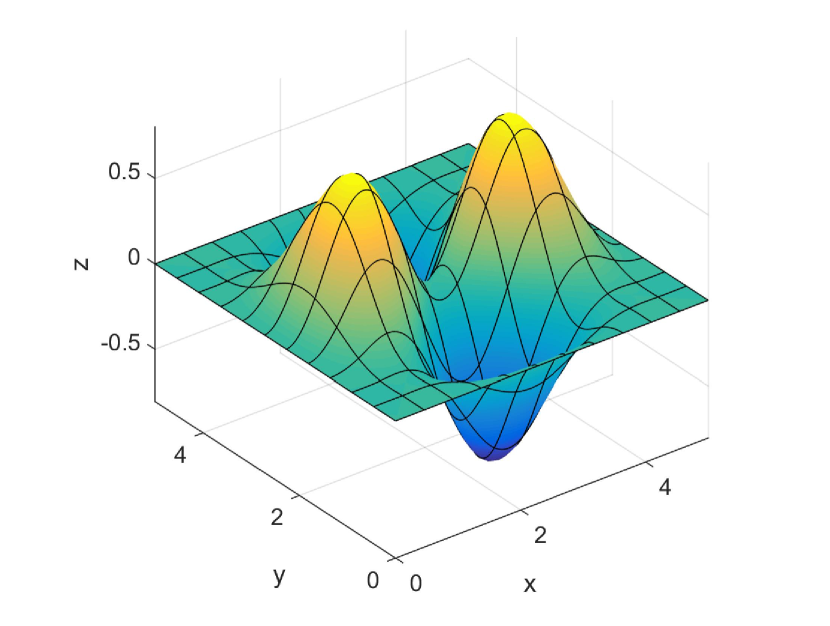
(e) $\bar{P}_{5}=78.9774$.

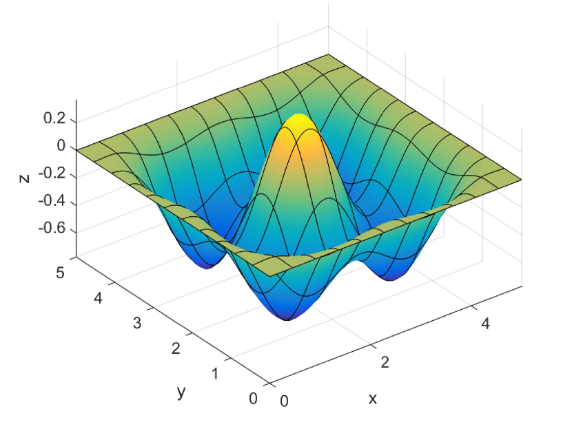
(f) $\bar{P}_{6}=84.1043$.

Figure 12: The first six buckling mode shapes of Al/Al₂O₃ CCCC square microplates.

Finally, this section ends up with a number of investigations on buckling behaviours of circular FG microplates. Table 16 presents the results of critical buckling load of CCCC Al/ZrO₂-2 circular plates without considering couple stress effects. It should be noted that, for this particular attempt of comparison purpose, the material volumes are defined as $V_{m}=\left(0.5-z/h\right)^{n}$ and $V_{c}=1-V_{m}$ [89, 90, 61, 68]. The comparison reveals that the results generated from proposed RPT are in good agreement with those of other shear deformation theories even with relatively thick and thick plates. The proposed quasi-3D yields slightly different results in all cases.

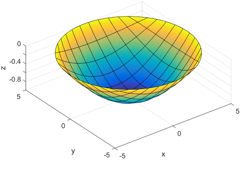
(a) $\bar{P}_{1}=10.7545$.

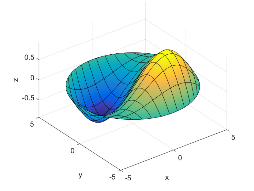
(b) $\bar{P}_{2}=49.5358$.

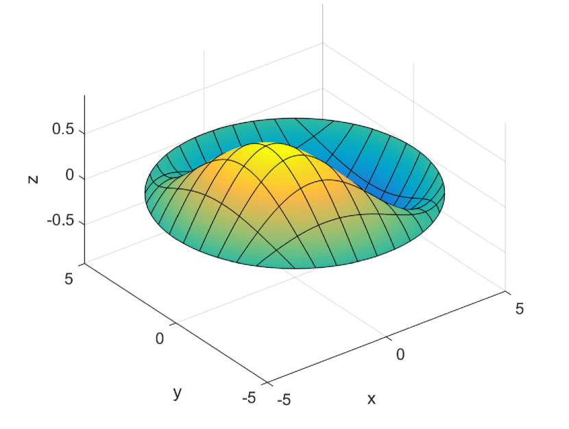
(c) $\bar{P}_{3}=49.5358$.

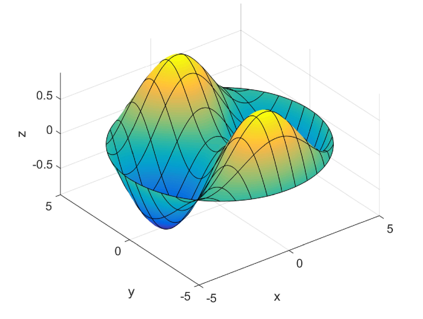
(d) $\bar{P}_{4}=80.6606$.

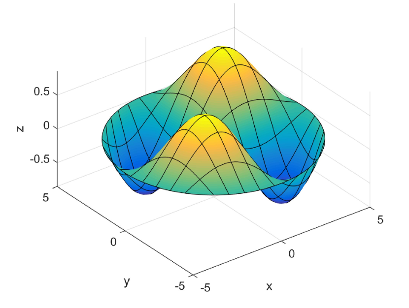
(e) $\bar{P}_{5}=104.8026$.

(f) $\bar{P}_{6}=108.1436$.

Figure 14: The first six buckling mode shapes of simply-supported Al/Al₂O₃ circular microplates.

Table 17 presents the non-dimensional critical buckling load of Al/Al₂O₃ circular microplates with various boundary conditions based on the proposed RPT and quasi-3D theories. The difference between the two theories is relatively small for both case of boundary conditions. The effects of material index $n$ and material length scale ratio $l/h$ on the critical buckling load of simply and clamped support of Al/Al₂O₃ circular microplates with $h/R=0.2$ are illustrated in Fig. 13. The first six buckling loads of Al/Al₂O₃ circular microplates with various aspects ratios for $n=1$ and $l/h=0.6$ along with the results generated from Zenkour’s quasi-3D theory [81] using proposed IGA approach are reported in Table 18. Six scaled buckling mode shapes corresponding to simply-supported circular microplates for $h/R=0.2$ based on proposed quasi-3D theory are presented in Fig. 14.

Table 16: Comparison of non-dimensional critical buckling load $\bar{P_{cr}}=\dfrac{P_{cr}R^{2}}{D_{m}}$ of CCCC Al/ZrO₂-2 circular plates (rule of mixtures scheme)

$n$	Theory	$h/R$
		0.1	0.2	0.25	0.3
0	TSDT [89]	14.089	12.574	11.638	10.670
	UTSDT [90]	14.089	12.575	11.639	10.670
	TSDT [68]	14.1089	12.5914	11.6540	10.6842
	RPT [61]	14.2023	12.7281	11.8143	10.8666
	RPT (Present)	14.0932	12.5776	11.6409	10.6719
	Quasi-3D (Present)	14.8264	13.4557	12.4564	11.3775
0.5	TSDT [89]	19.411	17.311	16.013	14.672
	UTSDT [90]	19.413	17.310	16.012	14.672
	TSDT [68]	19.4391	17.3327	16.0334	14.6910
	RPT [61]	19.5663	17.5180	16.2506	14.9381
	RPT (Present)	19.4169	17.3133	16.0153	14.6740
	Quasi-3D (Present)	20.5166	18.6074	17.2206	15.7222
2	TSDT [89]	23.074	20.803	19.377	17.882
	UTSDT [90]	23.075	20.805	19.378	17.881
	TSDT [68]	23.1062	20.8319	19.4033	17.9060
	RPT [61]	23.2592	21.0569	19.6687	18.2099
	RPT (Present)	23.0809	20.8088	19.3812	17.8848
	Quasi-3D (Present)	24.4332	22.3510	20.8035	19.1161
5	TSDT [89]	25.439	22.971	21.414	19.780
	UTSDT [90]	25.442	22.969	21.412	19.778
	TSDT [68]	25.4743	22.9992	21.4407	19.8043
	RPT [61]	25.6418	23.2426	21.7268	20.1313
	RPT (Present)	25.4469	22.9742	21.4168	19.7813
	Quasi-3D (Present)	26.8812	24.6195	22.9303	21.0878
10	TSDT [89]	27.133	24.423	22.725	20.948
	UTSDT [90]	27.131	24.422	22.725	20.949
	TSDT [68]	27.1684	24.4542	22.7536	20.9750
	RPT [61]	27.3429	24.6994	23.0389	21.2986
	RPT (Present)	27.1395	24.4287	22.7297	20.9524
	Quasi-3D (Present)	28.6197	26.1483	24.3140	22.3196

Table 17: Non-dimensional critical buckling load $\bar{P_{cr}}=\dfrac{P_{cr}R^{2}}{D_{m}}$ of Al/Al₂O₃ circular microplates (Mori-Tanaka scheme)

$h/R$	$l/h$	$n=0$			$n=1$			$n=10$
		RPT	Quasi-3D		RPT	Quasi-3D		RPT	Quasi-3D
Simple support
0.1	0	22.5182	22.6953		9.5368	9.7960		5.9574	6.0309
	0.2	23.0489	23.2627		9.8179	10.0793		6.0876	6.1617
	0.4	24.1022	24.4172		10.3474	10.6292		6.3543	6.4360
	0.6	25.0682	25.5337		10.8125	11.1391		6.6130	6.7163
	0.8	25.7985	26.4629		11.1543	11.5512		6.8182	6.9619
	1	26.3291	27.2420		11.3981	11.8897		6.9718	7.1752
0.2	0	21.7456	22.0263		9.2059	9.4510		5.6942	5.7510
	0.2	22.2719	22.5928		9.4873	9.7327		5.8318	5.8833
	0.4	23.2739	23.7059		9.9893	10.2520		6.1019	6.1509
	0.6	24.2066	24.8190		10.4423	10.7545		6.3676	6.4377
	0.8	24.9581	25.8386		10.8003	11.2074		6.5891	6.7170
	1	25.5480	26.7897		11.0777	11.6254		6.7647	6.9866
0.3	0	20.5707	20.8606		8.7033	8.9036		5.3041	5.3287
	0.2	21.0993	21.4128		8.9860	9.1777		5.4526	5.4621
	0.4	22.0854	22.4669		9.4810	9.6686		5.7409	5.7276
	0.6	23.0439	23.5641		9.9511	10.1693		6.0352	6.0281
	0.8	23.8746	24.6485		10.3517	10.6610		6.2927	6.3431
	1	24.5707	25.7228		10.6823	11.1443		6.5055	6.6623
Clamped support
0.1	0	76.5059	80.4859		30.4539	32.7398		19.7743	20.9413
	0.2	86.3696	90.4095		34.8524	37.1578		22.0235	23.1967
	0.4	115.9595	120.0466		48.0474	50.3612		28.7616	29.9236
	0.6	165.2737	169.2564		70.0379	72.3004		39.9728	41.0821
	0.8	234.3115	237.9906		100.8235	102.9597		55.6486	56.6598
	1	323.0727	326.2293		140.4042	142.3316		75.7879	76.6551
0.2	0	68.2782	73.0452		27.3245	29.8617		17.1442	18.6240
	0.2	77.6521	82.3859		31.5460	34.0702		19.3412	20.7979
	0.4	105.7687	110.0650		44.2098	46.5462		25.9122	27.1925
	0.6	152.6199	155.7501		65.3154	67.1544		36.8218	37.7110
	0.8	218.1997	219.2330		94.8629	95.8167		52.0495	52.3297
	1	302.5060	300.3159		132.8523	132.4584		71.5905	71.0373
0.3	0	57.9331	61.7636		23.3438	25.4648		14.0464	15.3047
	0.2	66.6302	70.2136		27.3083	29.3268		16.1359	17.3213
	0.4	92.7032	95.0207		39.2004	40.6571		22.3875	23.1508
	0.6	136.1160	135.6444		59.0182	59.2280		32.7704	32.6634
	0.8	196.8399	191.6493		86.7603	84.8742		47.2643	45.8312
	1	274.8619	262.6208		122.4264	117.4429		65.8628	62.6312

(a) Simply support.

(b) Clamped support.

Figure 13: Effects of material index $n$ and material length scale ratio $l/h$ on the critical buckling load of Al/Al₂O₃ circular microplates, $h/R=0.2$ (Mori-Tanaka scheme).

Table 18: The first six non-dimensional buckling loads $\bar{P}=\dfrac{PR^{2}}{D_{m}}$ of Al/Al₂O₃ circular microplates, $n=1$, $l/h=0.6$ (Mori-Tanaka scheme)

BC	$h/R$	Theory	Mode
			1	2	3	4	5	6
Simple support	0.1	IGA-Zenkour	11.4689	54.8031	54.8031	95.3143	123.2488	129.6396
		Quasi-3D (Present)	11.1391	54.0884	54.0884	93.7842	122.0854	128.1298
		RPT (Present)	10.8125	53.6215	53.6215	93.3944	122.3489	128.3281
	0.2	IGA-Zenkour	11.3113	50.7663	50.7663	83.1176	107.1987	110.9343
		Quasi-3D (Present)	10.7545	49.5358	49.5358	80.6606	104.8026	108.1436
		RPT (Present)	10.4423	50.2378	50.2378	83.3889	109.1766	112.9355
	0.3	IGA-Zenkour	10.8014	45.2015	45.2015	69.1649	89.4125	90.9795
		Quasi-3D (Present)	10.1693	43.6917	43.6917	66.3080	86.1911	87.4685
		RPT (Present)	9.9511	45.6739	45.6739	71.5215	93.8041	95.5819
Clamped support	0.1	IGA-Zenkour	72.6509	126.0657	126.0657	172.3464	205.4419	222.4846
		Quasi-3D (Present)	72.3004	125.7477	125.7477	171.5372	205.0589	221.0537
		RPT (Present)	70.0379	123.1185	123.1185	169.2944	203.3425	218.6139
	0.2	IGA-Zenkour	66.8949	108.9270	108.9270	140.4481	166.8569	175.2599
		Quasi-3D (Present)	67.1544	108.3685	108.3685	138.0488	164.4947	172.3137
		RPT (Present)	65.3154	109.4813	109.4813	143.4150	171.7706	179.5962
	0.3	IGA-Zenkour	58.9576	90.1444	90.1444	110.5155	131.5270	134.2574
		Quasi-3D (Present)	59.2280	88.4285	88.4285	106.6289	127.0395	129.6436
		RPT (Present)	59.0182	93.6789	93.6789	117.0824	140.3857	143.1361

5 Conclusions

In this study, a novel computational approach, which employs the modified couple stress theory, the four-variable refined plate theory and quasi-3D, and the NURBS-based isogemetric analysis, has been presented to investigate the static bending, free vibration, and buckling behaviours of functionally graded microplates with various geometric domains and boundary conditions. Within this proposed approach, the mathematical model governing the behaviours of the plates is constructed based on the modified couple stress theory with only one material length scale which efficiently taken into account the size-dependent effects of small-scale structures and the novel seventh-order refined plate theory and quasi-3D theory with only four unknowns. This proposed quasi-3D not only considers shear deformations but also is able to well capture the thickness stretching effect which is neglected by other classical, higher-order shear deformation, and refined plate theories. The NURBS-based isogeometric analysis is incorporated within the computational process to exactly describe the geometry an approximately construct the unknown field in which higher-order derivatives and continuity elements are readily satisfied. A large number of investigations including some benchmark examples have confirmed the validity and efficiency of the proposed approach. The obtained results also reveal that the increase of the material length scale parameter rises the microplates’ stiffness which results in the decline in the central displacement and increase in the natural frequency and buckling load. On the contrary, the growth of the material index leads to completely reverse trends in which microplates’ stiffness are fallen. Meanwhile, the numerical results that are generated by the proposed refined plate theory and quasi-3D theory are slightly different due to the consideration of the thickness stretching effect. However, these discrepancies become gradually vague as the microplates get thinner.

References

- [1] L. C. Trinh, T. P. Vo, A. I. Osofero, J. Lee, Fundamental frequency analysis of functionally graded sandwich beams based on the state space approach, Composite Structuresdoi:10.1016/j.compstruct.2015.11.010.
- [2] T. P. Vo, H.-T. Thai, T.-K. Nguyen, A. Maheri, J. Lee, Finite element model for vibration and buckling of functionally graded sandwich beams based on a refined shear deformation theory, Engineering Structures 64 (2014) 12–22. doi:10.1016/j.engstruct.2014.01.029.
- [3] T. P. Vo, H.-T. Thai, T.-K. Nguyen, F. Inam, Static and vibration analysis of functionally graded beams using refined shear deformation theory, Meccanica 49 (1) (2013) 155–168. doi:10.1007/s11012-013-9780-1.
- [4] M. Asghari, M. T. Ahmadian, M. H. Kahrobaiyan, M. Rahaeifard, On the size-dependent behavior of functionally graded micro-beams, Materials & Design 31 (5) (2010) 2324–2329. doi:10.1016/j.matdes.2009.12.006.
- [5] V.-H. Nguyen, T.-K. Nguyen, H.-T. Thai, T. P. Vo, A new inverse trigonometric shear deformation theory for isotropic and functionally graded sandwich plates, Composites Part B: Engineering 66 (2014) 233–246. doi:10.1016/j.compositesb.2014.05.012.
- [6] H.-T. Thai, T. P. Vo, A new sinusoidal shear deformation theory for bending, buckling, and vibration of functionally graded plates, Applied Mathematical Modelling 37 (5) (2013) 3269–3281. doi:10.1016/j.apm.2012.08.008.
- [7] A. M. Zenkour, Generalized shear deformation theory for bending analysis of functionally graded plates, Applied Mathematical Modelling 30 (1) (2006) 67 – 84. doi:http://dx.doi.org/10.1016/j.apm.2005.03.009.
- [8] J. N. Reddy, Analysis of functionally graded plates, International Journal for Numerical Methods in Engineering 47 (1-3) (2000) 663–684. doi:10.1002/(SICI)1097-0207(20000110/30)47:1/3<663::AID-NME787>3.0.CO;2-8.
- [9] J. L. Mantari, Refined and generalized hybrid type quasi-3d shear deformation theory for the bending analysis of functionally graded shells, Composites Part B: Engineering 83 (2015) 142–152. doi:10.1016/j.compositesb.2015.08.048.
- [10] J. Torabi, Y. Kiani, M. R. Eslami, Linear thermal buckling analysis of truncated hybrid FGM conical shells, Composites Part B: Engineering 50 (2013) 265–272. doi:10.1016/j.compositesb.2013.02.025.
- [11] F. Tornabene, Free vibration analysis of functionally graded conical, cylindrical shell and annular plate structures with a four-parameter power-law distribution, Computer Methods in Applied Mechanics and Engineering 198 (37–40) (2009) 2911–2935. doi:10.1016/j.cma.2009.04.011.
- [12] Y. Fu, H. Du, W. Huang, S. Zhang, M. Hu, TiNi-based thin films in MEMS applications: a review, Sensors and Actuators A: Physical 112 (2–3) (2004) 395–408. doi:10.1016/j.sna.2004.02.019.
- [13] Z. Lee, C. Ophus, L. M. Fischer, N. Nelson-Fitzpatrick, K. L. Westra, S. Evoy, V. Radmilovic, U. Dahmen, D. Mitlin, Metallic NEMS components fabricated from nanocomposite Al–Mo films, Nanotechnology 17 (12) (2006) 3063. doi:10.1088/0957-4484/17/12/042.
- [14] R. H. Baughman, C. Cui, A. A. Zakhidov, Z. Iqbal, J. N. Barisci, G. M. Spinks, G. G. Wallace, A. Mazzoldi, D. D. Rossi, A. G. Rinzler, O. Jaschinski, S. Roth, M. Kertesz, Carbon Nanotube Actuators, Science 284 (5418) (1999) 1340–1344. doi:10.1126/science.284.5418.1340.
- [15] K.-T. Lau, H.-Y. Cheung, J. Lu, Y.-S. Yin, D. Hui, H.-L. Li, Carbon Nanotubes for Space and Bio-Engineering Applications, Journal of Computational and Theoretical Nanoscience 5 (1) (2008) 23–35. doi:10.1166/jctn.2008.003.
- [16] S. J. V. Frankland, A. Caglar, D. W. Brenner, M. Griebel, Molecular Simulation of the Influence of Chemical Cross-Links on the Shear Strength of Carbon Nanotube−Polymer Interfaces, The Journal of Physical Chemistry B 106 (12) (2002) 3046–3048. doi:10.1021/jp015591+.
- [17] K. M. Liew, X. Q. He, C. H. Wong, On the study of elastic and plastic properties of multi-walled carbon nanotubes under axial tension using molecular dynamics simulation, Acta Materialia 52 (9) (2004) 2521–2527. doi:10.1016/j.actamat.2004.01.043.
- [18] N. A. Fleck, G. M. Muller, M. F. Ashby, J. W. Hutchinson, Strain gradient plasticity: Theory and experiment, Acta Metallurgica et Materialia 42 (2) (1994) 475–487. doi:10.1016/0956-7151(94)90502-9.
- [19] J. S. Stölken, A. G. Evans, A microbend test method for measuring the plasticity length scale, Acta Materialia 46 (14) (1998) 5109–5115. doi:10.1016/S1359-6454(98)00153-0.
- [20] D. Lam, F. Yang, A. Chong, J. Wang, P. Tong, Experiments and theory in strain gradient elasticity, Journal of the Mechanics and Physics of Solids 51 (8) (2003) 1477 – 1508. doi:http://dx.doi.org/10.1016/S0022-5096(03)00053-X.
- [21] A. C. Eringen, Nonlocal polar elastic continua, International Journal of Engineering Science 10 (1) (1972) 1–16. doi:10.1016/0020-7225(72)90070-5.
- [22] N. A. Fleck, J. W. Hutchinson, A phenomenological theory for strain gradient effects in plasticity, Journal of the Mechanics and Physics of Solids 41 (12) (1993) 1825–1857. doi:10.1016/0022-5096(93)90072-N.
- [23] F. Yang, A. C. M. Chong, D. C. C. Lam, P. Tong, Couple stress based strain gradient theory for elasticity, International Journal of Solids and Structures 39 (10) (2002) 2731–2743. doi:10.1016/S0020-7683(02)00152-X.
- [24] R. D. Mindlin, H. F. Tiersten, Effects of couple-stresses in linear elasticity, Archive for Rational Mechanics and Analysis 11 (1) (1962) 415–448. doi:10.1007/BF00253946.
- [25] R. D. Mindlin, Second gradient of strain and surface-tension in linear elasticity, International Journal of Solids and Structures 1 (4) (1965) 417–438. doi:10.1016/0020-7683(65)90006-5.
- [26] R. Ansari, R. Gholami, M. Faghih Shojaei, V. Mohammadi, S. Sahmani, Size-dependent bending, buckling and free vibration of functionally graded timoshenko microbeams based on the most general strain gradient theory, Composite Structures 100 (2013) 385–397. doi:10.1016/j.compstruct.2012.12.048.
- [27] S. K. Park, X.-L. Gao, Variational formulation of a modified couple stress theory and its application to a simple shear problem, Zeitschrift für angewandte Mathematik und Physik 59 (5) (2007) 904–917. doi:10.1007/s00033-006-6073-8.
- [28] S. K. Park, X.-L. Gao, Bernoulli–Euler beam model based on a modified couple stress theory, Journal of Micromechanics and Microengineering 16 (11) (2006) 2355. doi:10.1088/0960-1317/16/11/015.
- [29] W. Xia, L. Wang, L. Yin, Nonlinear non-classical microscale beams: Static bending, postbuckling and free vibration, International Journal of Engineering Science 48 (12) (2010) 2044–2053. doi:10.1016/j.ijengsci.2010.04.010.
- [30] L.-L. Ke, Y.-S. Wang, Size effect on dynamic stability of functionally graded microbeams based on a modified couple stress theory, Composite Structures 93 (2) (2011) 342–350. doi:10.1016/j.compstruct.2010.09.008.
- [31] C. M. C. Roque, D. S. Fidalgo, A. J. M. Ferreira, J. N. Reddy, A study of a microstructure-dependent composite laminated Timoshenko beam using a modified couple stress theory and a meshless method, Composite Structures 96 (2013) 532–537. doi:10.1016/j.compstruct.2012.09.011.
- [32] H.-T. Thai, T. P. Vo, T.-K. Nguyen, J. Lee, Size-dependent behavior of functionally graded sandwich microbeams based on the modified couple stress theory, Composite Structures 123 (2015) 337–349. doi:10.1016/j.compstruct.2014.11.065.
- [33] M. Salamat-talab, A. Nateghi, J. Torabi, Static and dynamic analysis of third-order shear deformation FG micro beam based on modified couple stress theory, International Journal of Mechanical Sciences 57 (1) (2012) 63–73. doi:10.1016/j.ijmecsci.2012.02.004.
- [34] G. C. Tsiatas, A new Kirchhoff plate model based on a modified couple stress theory, International Journal of Solids and Structures 46 (13) (2009) 2757–2764. doi:10.1016/j.ijsolstr.2009.03.004.
- [35] L. Yin, Q. Qian, L. Wang, W. Xia, Vibration analysis of microscale plates based on modified couple stress theory, Acta Mechanica Solida Sinica 23 (5) (2010) 386 – 393. doi:http://dx.doi.org/10.1016/S0894-9166(10)60040-7.
- [36] H. M. Ma, X.-L. Gao, J. N. Reddy, A non-classical Mindlin plate model based on a modified couple stress theory, Acta Mechanica 220 (1-4) (2011) 217–235. doi:10.1007/s00707-011-0480-4.
- [37] M. Simsek, T. Kocaturk, S. D. Akbas, Static bending of a functionally graded microscale Timoshenko beam based on the modified couple stress theory, Composite Structures 95 (2013) 740–747. doi:10.1016/j.compstruct.2012.08.036.
- [38] A. Nateghi, M. Salamat-talab, J. Rezapour, B. Daneshian, Size dependent buckling analysis of functionally graded micro beams based on modified couple stress theory, Applied Mathematical Modelling 36 (10) (2012) 4971–4987. doi:10.1016/j.apm.2011.12.035.
- [39] J. N. Reddy, J. Kim, A nonlinear modified couple stress-based third-order theory of functionally graded plates, Composite Structures 94 (3) (2012) 1128–1143. doi:10.1016/j.compstruct.2011.10.006.
- [40] J. N. Reddy, J. Berry, Nonlinear theories of axisymmetric bending of functionally graded circular plates with modified couple stress, Composite Structures 94 (12) (2012) 3664–3668. doi:10.1016/j.compstruct.2012.04.019.
- [41] J. Kim, J. N. Reddy, A general third-order theory of functionally graded plates with modified couple stress effect and the von karman nonlinearity: theory and finite element analysis, Acta Mechanica 226 (9) (2015) 2973–2998. doi:10.1007/s00707-015-1370-y.
- [42] J. N. Reddy, J. Romanoff, J. A. Loya, Nonlinear Finite Element Analysis of Functionally Graded Circular Plates with Modified Couple Stress Theory, European Journal of Mechanics - A/Solidsdoi:10.1016/j.euromechsol.2015.11.001.
- [43] H.-T. Thai, S.-E. Kim, A size-dependent functionally graded reddy plate model based on a modified couple stress theory, Composites Part B: Engineering 45 (1) (2013) 1636 – 1645. doi:http://dx.doi.org/10.1016/j.compositesb.2012.09.065.
- [44] H.-T. Thai, D.-H. Choi, Size-dependent functionally graded kirchhoff and mindlin plate models based on a modified couple stress theory, Composite Structures 95 (2013) 142 – 153. doi:http://dx.doi.org/10.1016/j.compstruct.2012.08.023.
- [45] H.-T. Thai, T. P. Vo, A size-dependent functionally graded sinusoidal plate model based on a modified couple stress theory, Composite Structures 96 (2013) 376–383. doi:10.1016/j.compstruct.2012.09.025.
- [46] L.-L. Ke, Y.-S. Wang, J. Yang, S. Kitipornchai, Free vibration of size-dependent Mindlin microplates based on the modified couple stress theory, Journal of Sound and Vibration 331 (1) (2012) 94–106. doi:10.1016/j.jsv.2011.08.020.
- [47] L.-L. Ke, J. Yang, S. Kitipornchai, M. A. Bradford, Bending, buckling and vibration of size-dependent functionally graded annular microplates, Composite Structures 94 (11) (2012) 3250–3257. doi:10.1016/j.compstruct.2012.04.037.
- [48] L. He, J. Lou, E. Zhang, Y. Wang, Y. Bai, A size-dependent four variable refined plate model for functionally graded microplates based on modified couple stress theory, Composite Structures 130 (2015) 107 – 115. doi:http://dx.doi.org/10.1016/j.compstruct.2015.04.033.
- [49] L. Della Croce, P. Venini, Finite elements for functionally graded Reissner–Mindlin plates, Computer Methods in Applied Mechanics and Engineering 193 (9–11) (2004) 705–725. doi:10.1016/j.cma.2003.09.014.
- [50] H. Nguyen-Xuan, G. R. Liu, C. Thai-Hoang, T. Nguyen-Thoi, An edge-based smoothed finite element method (ES-FEM) with stabilized discrete shear gap technique for analysis of Reissner–Mindlin plates, Computer Methods in Applied Mechanics and Engineering 199 (9–12) (2010) 471–489. doi:10.1016/j.cma.2009.09.001.
- [51] B. Zhang, Y. He, D. Liu, Z. Gan, L. Shen, A non-classical Mindlin plate finite element based on a modified couple stress theory, European Journal of Mechanics - A/Solids 42 (2013) 63–80. doi:10.1016/j.euromechsol.2013.04.005.
- [52] J. N. Reddy, A Simple Higher-Order Theory for Laminated Composite Plates, Journal of Applied Mechanics 51 (4) (1984) 745–752. doi:10.1115/1.3167719.
- [53] H. Nguyen-Xuan, C. H. Thai, T. Nguyen-Thoi, Isogeometric finite element analysis of composite sandwich plates using a higher order shear deformation theory, Composites Part B: Engineering 55 (2013) 558–574. doi:10.1016/j.compositesb.2013.06.044.
- [54] H. Arya, R. P. Shimpi, N. K. Naik, A zigzag model for laminated composite beams, Composite Structures 56 (1) (2002) 21–24. doi:10.1016/S0263-8223(01)00178-7.
- [55] N. R. Senthilnathan, S. P. Lim, K. H. Lee, S. T. Chow, Buckling of Shear-Deformable Plates, AIAA Journal 25 (9) (1987) 1268–1271. doi:10.2514/3.48742.
- [56] R. P. Shimpi, Refined plate theory and its variants, AIAA journal 40 (1) (2002) 137–146.
- [57] R. P. Shimpi, H. G. Patel, A two variable refined plate theory for orthotropic plate analysis, International Journal of Solids and Structures 43 (22–23) (2006) 6783–6799. doi:10.1016/j.ijsolstr.2006.02.007.
- [58] R. P. Shimpi, H. G. Patel, Free vibrations of plate using two variable refined plate theory, Journal of Sound and Vibration 296 (4–5) (2006) 979–999. doi:10.1016/j.jsv.2006.03.030.
- [59] C. A. Shankara, N. G. R. Iyengar, A C0 element for the free vibration analysis of laminated composite plates, Journal of Sound and Vibration 191 (5) (1996) 721–738. doi:10.1006/jsvi.1996.0152.
- [60] T. Hughes, J. Cottrell, Y. Bazilevs, Isogeometric analysis: Cad, finite elements, nurbs, exact geometry and mesh refinement, Computer Methods in Applied Mechanics and Engineering 194 (39–41) (2005) 4135 – 4195. doi:http://dx.doi.org/10.1016/j.cma.2004.10.008.
- [61] H. Nguyen-Xuan, L. V. Tran, C. H. Thai, S. Kulasegaram, S. Bordas, Isogeometric analysis of functionally graded plates using a refined plate theory, Composites Part B: Engineering 64 (2014) 222 – 234. doi:http://dx.doi.org/10.1016/j.compositesb.2014.04.001.
- [62] A. V. Vuong, C. Heinrich, B. Simeon, ISOGAT: A 2d tutorial MATLAB code for Isogeometric Analysis, Computer Aided Geometric Design 27 (8) (2010) 644–655. doi:10.1016/j.cagd.2010.06.006.
- [63] C. de Falco, A. Reali, R. Vázquez, GeoPDEs: A research tool for Isogeometric Analysis of PDEs, Advances in Engineering Software 42 (12) (2011) 1020–1034. doi:10.1016/j.advengsoft.2011.06.010.
- [64] V. P. Nguyen, C. Anitescu, S. P. A. Bordas, T. Rabczuk, Isogeometric analysis: An overview and computer implementation aspects, Mathematics and Computers in Simulation 117 (2015) 89–116. doi:10.1016/j.matcom.2015.05.008.
- [65] D. Wang, W. Liu, H. Zhang, Superconvergent isogeometric free vibration analysis of Euler–Bernoulli beams and Kirchhoff plates with new higher order mass matrices, Computer Methods in Applied Mechanics and Engineering 286 (2015) 230–267. doi:10.1016/j.cma.2014.12.026.
- [66] L. Beirão da Veiga, A. Buffa, C. Lovadina, M. Martinelli, G. Sangalli, An isogeometric method for the Reissner–Mindlin plate bending problem, Computer Methods in Applied Mechanics and Engineering 209–212 (2012) 45–53. doi:10.1016/j.cma.2011.10.009.
- [67] C. H. Thai, H. Nguyen-Xuan, N. Nguyen-Thanh, T.-H. Le, T. Nguyen-Thoi, T. Rabczuk, Static, free vibration, and buckling analysis of laminated composite Reissner–Mindlin plates using NURBS-based isogeometric approach, International Journal for Numerical Methods in Engineering 91 (6) (2012) 571–603. doi:10.1002/nme.4282.
- [68] L. V. Tran, A. Ferreira, H. Nguyen-Xuan, Isogeometric analysis of functionally graded plates using higher-order shear deformation theory, Composites Part B: Engineering 51 (2013) 368 – 383. doi:http://dx.doi.org/10.1016/j.compositesb.2013.02.045.
- [69] C. H. Thai, A. J. M. Ferreira, E. Carrera, H. Nguyen-Xuan, Isogeometric analysis of laminated composite and sandwich plates using a layerwise deformation theory, Composite Structures 104 (2013) 196–214. doi:10.1016/j.compstruct.2013.04.002.
- [70] L. V. Tran, C. H. Thai, H. Nguyen-Xuan, An isogeometric finite element formulation for thermal buckling analysis of functionally graded plates, Finite Elements in Analysis and Design 73 (2013) 65–76. doi:10.1016/j.finel.2013.05.003.
- [71] P. Phung-Van, M. Abdel-Wahab, K. M. Liew, S. P. A. Bordas, H. Nguyen-Xuan, Isogeometric analysis of functionally graded carbon nanotube-reinforced composite plates using higher-order shear deformation theory, Composite Structures 123 (2015) 137–149. doi:10.1016/j.compstruct.2014.12.021.
- [72] L. V. Tran, J. Lee, H. Nguyen-Van, H. Nguyen-Xuan, M. A. Wahab, Geometrically nonlinear isogeometric analysis of laminated composite plates based on higher-order shear deformation theory, International Journal of Non-Linear Mechanics 72 (2015) 42–52. doi:10.1016/j.ijnonlinmec.2015.02.007.
- [73] C. H. Thai, H. Nguyen-Xuan, S. P. A. Bordas, N. Nguyen-Thanh, T. Rabczuk, Isogeometric Analysis of Laminated Composite Plates Using the Higher-Order Shear Deformation Theory, Mechanics of Advanced Materials and Structures 22 (6) (2015) 451–469. doi:10.1080/15376494.2013.779050.
- [74] S. S. Vel, R. C. Batra, Exact Solution for Thermoelastic Deformations of Functionally Graded Thick Rectangular Plates, AIAA Journal 40 (7) (2002) 1421–1433. doi:10.2514/2.1805.
- [75] L. F. Qian, R. C. Batra, L. M. Chen, Static and dynamic deformations of thick functionally graded elastic plates by using higher-order shear and normal deformable plate theory and meshless local Petrov–Galerkin method, Composites Part B: Engineering 35 (6–8) (2004) 685–697. doi:10.1016/j.compositesb.2004.02.004.
- [76] T. Mori, K. Tanaka, Average stress in matrix and average elastic energy of materials with misfitting inclusions, Acta Metallurgica 21 (5) (1973) 571–574. doi:10.1016/0001-6160(73)90064-3.
- [77] Y. Kiani, M. R. Eslami, Thermal Postbuckling of Imperfect Circular Functionally Graded Material Plates: Examination of Voigt, Mori–Tanaka, and Self-Consistent Schemes, Journal of Pressure Vessel Technology 137 (2) (2014) 021201–021201. doi:10.1115/1.4026993.
- [78] E. Carrera, S. Brischetto, M. Cinefra, M. Soave, Effects of thickness stretching in functionally graded plates and shells, Composites Part B: Engineering 42 (2) (2011) 123 – 133. doi:http://dx.doi.org/10.1016/j.compositesb.2010.10.005.
- [79] J. L. Mantari, C. Guedes Soares, A novel higher-order shear deformation theory with stretching effect for functionally graded plates, Composites Part B: Engineering 45 (1) (2013) 268–281. doi:10.1016/j.compositesb.2012.05.036.
- [80] C. H. Thai, A. M. Zenkour, M. Abdel Wahab, H. Nguyen-Xuan, A simple four-unknown shear and normal deformations theory for functionally graded isotropic and sandwich plates based on isogeometric analysis, Composite Structures 139 (2016) 77–95. doi:10.1016/j.compstruct.2015.11.066.
- [81] A. M. Zenkour, A simple four-unknown refined theory for bending analysis of functionally graded plates, Applied Mathematical Modelling 37 (2013) 9041 – 9051. doi:http://dx.doi.org/10.1016/j.apm.2013.04.022.
- [82] A. M. Zenkour, Bending analysis of functionally graded sandwich plates using a simple four-unknown shear and normal deformations theory, Journal of Sandwich Structures and Materials 15 (6) (2013) 629–656. doi:10.1177/1099636213498886.
- [83] T. N. Nguyen, C. H. Thai, H. Nguyen-Xuan, On the general framework of high order shear deformation theories for laminated composite plate structures: A novel unified approach, International Journal of Mechanical Sciencesdoi:10.1016/j.ijmecsci.2016.01.012.
- [84] J. N. Reddy, Theory and Analysis of Elastic Plates and Shells, 2nd Edition, CRC Press, 2006.
- [85] N.-T. Nguyen, D. Hui, J. Lee, H. Nguyen-Xuan, An efficient computational approach for size-dependent analysis of functionally graded nanoplates, Computer Methods in Applied Mechanics and Engineering 297 (2015) 191 – 218. doi:http://dx.doi.org/10.1016/j.cma.2015.07.021.
- [86] J. A. Cottrell, T. J. R. Hughes, Y. Bazilevs, Isogeometric Analysis: Toward Integration of CAD and FEA, 1st Edition, Wiley Publishing, 2009.
- [87] F. Auricchio, L. B. da Veiga, A. Buffa, C. Lovadina, A. Reali, G. Sangalli, A fully “locking-free” isogeometric approach for plane linear elasticity problems: A stream function formulation, Computer Methods in Applied Mechanics and Engineering 197 (1–4) (2007) 160 – 172. doi:http://dx.doi.org/10.1016/j.cma.2007.07.005.
- [88] M. Mohammadi, M. Ghayour, A. Farajpour, Free transverse vibration analysis of circular and annular graphene sheets with various boundary conditions using the nonlocal continuum plate model, Composites Part B: Engineering 45 (1) (2013) 32 – 42. doi:http://dx.doi.org/10.1016/j.compositesb.2012.09.011.
- [89] L. Ma, T. Wang, Relationships between axisymmetric bending and buckling solutions of {FGM} circular plates based on third-order plate theory and classical plate theory, International Journal of Solids and Structures 41 (1) (2004) 85 – 101. doi:http://dx.doi.org/10.1016/j.ijsolstr.2003.09.008.
- [90] A. Saidi, A. Rasouli, S. Sahraee, Axisymmetric bending and buckling analysis of thick functionally graded circular plates using unconstrained third-order shear deformation plate theory, Composite Structures 89 (1) (2009) 110 – 119. doi:http://dx.doi.org/10.1016/j.compstruct.2008.07.003.
- [91] H.-T. Thai, S.-E. Kim, A simple quasi-3d sinusoidal shear deformation theory for functionally graded plates, Composite Structures 99 (2013) 172–180. doi:10.1016/j.compstruct.2012.11.030.
- [92] A. Neves, A. Ferreira, E. Carrera, C. Roque, M. Cinefra, R. Jorge, C. Soares, A quasi-3d sinusoidal shear deformation theory for the static and free vibration analysis of functionally graded plates, Composites Part B: Engineering 43 (2) (2012) 711 – 725. doi:http://dx.doi.org/10.1016/j.compositesb.2011.08.009.
- [93] J. L. Mantari, C. G. Soares, A quasi-3d tangential shear deformation theory with four unknowns for functionally graded plates, Acta Mechanica 226 (3) (2014) 625–642. doi:10.1007/s00707-014-1192-3.
- [94] S. Akavci, A. Tanrikulu, Static and free vibration analysis of functionally graded plates based on a new quasi-3d and 2d shear deformation theories, Composites Part B: Engineering 83 (2015) 203 – 215. doi:http://dx.doi.org/10.1016/j.compositesb.2015.08.043.
- [95] S. S. Vel, R. Batra, Three-dimensional exact solution for the vibration of functionally graded rectangular plates, Journal of Sound and Vibration 272 (3–5) (2004) 703 – 730. doi:http://dx.doi.org/10.1016/S0022-460X(03)00412-7.
- [96] H. Matsunaga, Free vibration and stability of functionally graded plates according to a 2-d higher-order deformation theory, Composite Structures 82 (4) (2008) 499 – 512. doi:http://dx.doi.org/10.1016/j.compstruct.2007.01.030.
- [97] Z. Belabed, M. S. A. Houari, A. Tounsi, S. Mahmoud, O. A. Bég, An efficient and simple higher order shear and normal deformation theory for functionally graded material (fgm) plates, Composites Part B: Engineering 60 (2014) 274 – 283. doi:http://dx.doi.org/10.1016/j.compositesb.2013.12.057.
- [98] F. Alijani, M. Amabili, Effect of thickness deformation on large-amplitude vibrations of functionally graded rectangular plates, Composite Structures 113 (2014) 89 – 107. doi:http://dx.doi.org/10.1016/j.compstruct.2014.03.006.