Reliability of the optimized perturbation theory in the 0-dimensional $O(N)$ scalar field model

Abstract

We address the reliability of the Optimized Perturbation Theory (OPT) in the context of the 0-dimensional $O(N)$ scalar field model. The effective potential, the self-energy and the 1PI four-point Green’s function for the model are computed using different optimization schemes and the results contrasted to the exact results for the model. Our results are also compared to those obtained with the $1/N$-expansion and with those from ordinary perturbation theory. The OPT results are shown to be stable even at large couplings and to have better convergence properties than the ones produced in the $1/N$-expansion. It is also shown that the principle of minimal sensitive optimization procedure used in conjunction with the OPT method tends to always produce better results, in particular when applied directly to the self-energy.

1 Introduction

Perturbation theory is the most comprehensive way of studying nonlinear problems in physics area wide. However, it is a fact that not always we can rely on some small quantity in the theory which we can use as a parameter which we can perturb physical quantities of interest, or even when we do have, it is not warranted that a perturbative series might be well posed, i.e., converge after a few terms are considered. Most of the times we must make use of some nonperturbative method to get around these problems. One typical example where perturbation theory breaks down is in the studies of phase transitions in general, particularly close to a critical point. This can also happen due to the appearance of large infrared divergences [1], as in the case where massless modes are present, or close to a transition point in field theories displaying a second order phase transition [2] or a weakly first order transition [3]. In all these cases, the use of some reliable nonperturbative technique is required to proper study these systems. Among the analytical nonperturbative techniques, one can cite for example making use of a discretization of the system and studying it numerically (e.g., lattice simulations), make use of analytical methods like an expansion in the number of field components, $N$, in the case of field theory, using the $1/N$-approximation [4], among other methods.

In this work we want to access the reliability of one of those nonperturbative methods that have been used with some frequency in the literature: The optimized perturbation theory (OPT). The OPT is an analytical technique which allies the computational advantages of ordinary perturbation theory to a variational criterion in order to generate nonperturbative results [5]. The OPT method has been used extensively in the literature to treat many different physical systems, ranging from condensed matter problems, phase transition problems in finite temperature quantum field theory and others (see, e.g., Refs. [6, 7, 8, 9, 10, 11, 12, 13, 14, 15, 16, 17, 18, 19, 20, 21, 22] and references there in for some examples of applications).

When applying the OPT method to a gauge theory, a modified form of the method is required. In this case, a suitable modification preserving gauge invariance can be implemented. This modification of the OPT method is known in this case as the Hard Thermal Loop perturbation theory (HTLpt) (see, e.g., the original proposal in Ref. [23] and also the review [24]).

One particular issue regarding the OPT method that we would like to also address in this work regards the quantity to which one should apply the variational criterion as required by the method. In a calculation where different physical quantities are available, in the original proposal by Stevenson [25], the variational principle used was the principle of minimal sensitivity (PMS) and it was advocated that the PMS should be applied to each different physical quantity that is being computed, producing different optimized parameters. However, one could argue that the PMS should be applied to a more general quantity such as the ground-state energy density as in Ref. [26], or to the effective potential, which generates all one-particle irreducible contributions, as in Refs. [11, 13, 14, 15, 27], while previous works [28, 29] have shown that applying the PMS to the self-energy would be more appropriate. In this work we want to clarify in this issue of which quantity we should optimize in the OPT method and also which quantity can provide the best convergence in the OPT. With this aim we shall compare the results obtained by a direct optimization of the effective potential (the zero-point Green function), the self-energy (the two-point Green function) and also to the effective coupling (the four-point Green function) in the context of the 0-dimensional $O(N)$ scalar field theory model.

One should note that one of the main differences as far as a comparison to a quantum field theory model in $D>0$ is concerned, is the need to regularize and renormalize physical quantities, which is, of course, absent in the zero-dimensional model studied here. The renormalization group flow dictates the change of physical parameters with the scale and in this case the application of the OPT has to be handled very carefully [30, 31, 32]. Note, however, that the OPT method is not restricted to renormalizable models and it has been applied successfully to many effective nonrenormalizable models as well [26, 33, 34]. Even so, the application of the OPT to the present exact soluble model offers an unique opportunity to elucidate on the possible optimization criteria issues, which are not possible to perform in other models without exact solutions. Because of this, the 0-dimensional $O(N)$ scalar field theory model is the perfect benchmark toy model to use to perform different tests related to the application of the OPT method, but it also useful to test other different nonperturbative methods used in quantum field theory as well.

The remainder of this work is organized as follows. In Sec. 2, we briefly describe the 0-dimensional $O(N)$ scalar field model and show why perturbation theory might not be reliable in the context of this model in special. In Sec. 3, we introduce the OPT method and also describe three main variational tools that are commonly used in conjunction with this method. In Sec. 4, we perform a comparison between exact results and the nonperturbative results obtained by OPT. These results are also contrasted with those obtained from the $1/N$-expansion. This way we can better evaluate the usefulness of the OPT and the corresponding variational methods with this popular nonperturbative method. Our concluding remarks are given in Sec. 5. Four appendixes are included where we give some of the technical details.

2 The 0-dimensional $O(N)$ scalar field model

The 0-dimensional $O(N)$ scalar field model describes an $N$-component anharmonic oscillator in zero spacetime dimension, whose action is given by

$$S(\bm{\varphi}) = \frac{m}{2}{\bm{\varphi}}.{\bm{\varphi}}+\frac{\lambda}{4!}({\bm{\varphi}}.{\bm{\varphi}})^{2},$$ (1)

where $m,\lambda$ are real and positive parameters and ${\bm{\varphi}}\equiv(\varphi_{1},\ldots,\varphi_{N})$ is a scalar field with $N$ components. Equation (1) is an invariant under $O(N)$ rotations.

The generating function for the $n$-point Green’s functions is given by

$$Z\left({\bm{J}}\right)=\int D\bm{\varphi}\exp\left[{-S\left(\bm{\varphi}\right)+\bm{J}\cdot\bm{\varphi}}\right],$$ (2)

where $\bm{J}$ is an external source. From the generating function, the $n$-point Green functions are given by

$$G_{i_{1}\cdots i_{n}}^{(n)}=\left.\frac{1}{Z}\frac{\delta^{n}Z({\bm{J}})}{\delta J_{i_{1}}\cdots\delta J_{i_{n}}}\right|_{J_{i}=0}=\langle\varphi_{i_{1}}\cdots\varphi_{i_{n}}\rangle,$$ (3)

and averages are given by their standard definition,

$$\langle\cdots\rangle=\frac{\int\mathcal{D}\bm{\varphi}\exp[-S(\bm{\varphi})][\cdots]}{Z}.$$ (4)

The connected Green functions are obtained from the functional generator $W(\bf J)$, defined as [35]

$$W(\bm{J})=\ln\left[\frac{Z(\bm{J}\ )}{Z_{0}}\right],$$ (5)

where $Z_{0}$ is the normalization of the generating functional $Z_{0}=Z(\bm{J}=0)|_{\lambda=0}$. The connected Green functions are then given by

$$G_{c,{i_{1}}\ldots{i_{n}}}^{(n)}=\left.\frac{\delta^{n}W\left(\bm{J}\right)}{\delta J_{i_{1}}\ldots\delta J_{i_{n}}}\right|_{J_{i}=0}=\langle\varphi_{i_{1}}\ldots\varphi_{i_{n}}\rangle_{\rm connected}.$$ (6)

From the definition of the expectation value of the field,

$$\phi_{i}=\langle\varphi_{i}\rangle_{J_{i}}=\frac{\delta W}{\delta J_{i}},$$ (7)

we can perform the usual Legendre transformation and obtain the effective action, or the generation functional of the one-particle irreducible (1PI) Green’s functions [35]

$$\Gamma(\bm{\phi})=W(\bm{J})-\bm{J}\cdot\bm{\phi}.$$ (8)

The advantage of working with the 0-dimensional $O(N)$ scalar field model is that it has explicit analytical solution, which can be contrasted with different approximations used in the literature and, thus, it is a perfect benchmarking model to use. In this work, we will make use of the effective potential $V_{\rm eff}$, the self-energy $\Sigma$ and the 1PI four-point Green’s functions. The one-particle irreducible (1PI) Green’s functions, $\Gamma^{(n)}$, are defined by

$$\Gamma^{(n)}_{i_{1}\cdots i_{n}}=\left.-\frac{\delta^{n}\Gamma[\bm{\phi}]}{\delta\phi_{i_{1}}...\delta\phi_{i_{n}}}\right|_{\phi=0}$$ (9)

In particular, in the rest of this work we will make use of the effective potential, $V_{\rm eff}=-\ln Z$, the self-energy, $\Sigma\equiv\Gamma^{(2)}-m$ and the vertex function $\Gamma^{(4)}$.

Let us give the explicit expressions for these quantities for the present model. Starting with the partition function, ${Z}\equiv Z(0)$, given by [36, 37]

$$Z=\int\mathcal{D}\bm{\varphi}\ e^{-S(\bm{\varphi})}=\Omega_{N}\mathcal{R}_{N-1},$$ (10)

where $\Omega_{N}$ is the surface area in $N$-dimensional unit sphere,

$$\Omega_{N}=\frac{2\pi^{N/2}}{\Gamma\left(\frac{N}{2}\right)},$$ (11)

and $\mathcal{R}_{N}$ is defined by

$$\mathcal{R}_{N} = \int_{0}^{\infty}\ x^{N}\ e^{-\frac{m}{2}x^{2}-\frac{\lambda}{4!}x^{4}}dx$$ (12)

$$= 2^{\frac{3N-5}{4}}3^{\frac{N+1}{4}}\lambda^{-\frac{N+3}{4}}\left[\sqrt{\lambda}\Gamma\left(\frac{N+1}{4}\right)\right.$$

$$\times \left.\ {}_{1}F_{1}\left(\frac{N+1}{4};\frac{1}{2};\frac{3m^{2}}{2\lambda}\right)-\sqrt{6}m\Gamma\left(\frac{N+3}{4}\right)\right.$$

$$\times \left.\ {}_{1}F_{1}\left(\frac{N+3}{4};\frac{3}{2};\frac{3m^{2}}{2\lambda}\right)\right],$$

where ${}_{1}F_{1}\left(\alpha;\beta;z\right)$ is the Kummer confluent hypergeometric function [38].

The explicit exact solutions for $V_{\rm eff}$, $\Sigma$ and $\Gamma^{(4)}$ that we use throughout this work are then found to be given, respectively, by:

$$V_{\rm{eff}}^{\rm exact}=-\ln(\Omega_{N}\mathcal{R}_{N-1}),$$ (13)

$$\Sigma_{\rm exact}=N\frac{\mathcal{R}_{N-1}}{\mathcal{R}_{N+1}}-m,$$ (14)

$$\Gamma^{\left(4\right)}_{\rm exact}\!=\!-3N^{2}\!\left(\frac{\mathcal{R}_{N-1}}{\mathcal{R}_{N+1}}\right)^{2}\!\!\left[\frac{N(\mathcal{R}_{N+3})\left(\mathcal{R}_{N-1}\right)}{(N+2)\left(\mathcal{R}_{N+1}\right)^{2}}-1\right].$$ (15)

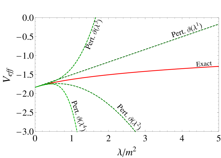
Figure 1: The effective potential $V_{\rm eff}$ for the model, considering $N=2$. The exact solution is given by the solid line. The results obtained by expanding $V_{\rm eff}$ in a power series in $\lambda/{m^{2}}$ are given by the dashed lines.

For illustrative purposes, we give in A the perturbative expansion (the power series expansion in the coupling constant $\lambda$) for the effective potential, $V_{\rm eff}$, the self-energy $\Sigma$ and the vertex function $\Gamma^{(4)}$. That this is not a well posed perturbative series (as far convergence is concerned) is shown in Fig. 1 for the particular case of the perturbative expansion for the effective potential. We can see that perturbative expansion shows no sign of converging. In fact, it can be shown that the series has a zero radius of convergence [39].

3 Optimized Perturbation Theory

The application of the OPT method starts by implementing a linear interpolation in the action,

$$S\rightarrow S_{\delta}=\left(1-\delta\right)S_{0}\left(\eta\right)+\delta S,$$ (16)

where $\delta$ is a fictitious expansion parameter, which is used only for bookkeeping purposes and set at the end equal to one. The parameter $\eta$ is an arbitrary mass term, fixed through an appropriate variational method. Some common ways of fixing this parameter will be described below. It is through this variational method that nonperturbative effects are included through the OPT mass parameter $\eta$. The OPT method has been successfully applied in different scenarios (see, e.g Refs. [6, 7, 8, 9, 10, 11, 13, 14, 15, 21, 40] and references there in). In this work, we apply this nonperturbative method to evaluate the $n$-point 1PI Green’s functions of the 0-dimensional $O(N)$ scalar field model described in the previous section. We compare the OPT results with the exact solution that this particular toy model gives. For comparison purposes we also contrast the OPT results with those obtained through another nonperturbative method, obtained with the $1/N$-expansion for the model.

Applying the interpolation (16) in Eq. (1) gives

$$S(\bm{\varphi}) = \frac{m}{2}\bm{\varphi}.\bm{\varphi}+(1-\delta)\frac{\eta}{2}\bm{\varphi}.\bm{\varphi}+\delta\frac{\lambda}{4!}(\bm{\varphi}.\bm{\varphi})^{2}$$ (17)

$$= S_{0}(\bm{\varphi},\eta)+S_{\delta}(\bm{\varphi},\eta),$$

where

$$S_{0}(\bm{\varphi},\eta)=\frac{m+\eta}{2}\bm{\varphi}.\bm{\varphi},$$ (18)

and

$$S_{\delta}(\bm{\varphi},\eta)=-\delta\frac{\eta}{2}\bm{\varphi}.\bm{\varphi}+\delta\frac{\lambda}{4!}(\bm{\varphi}.\bm{\varphi})^{2},$$ (19)

which is considered as the modified interaction term in the OPT method.

In the OPT method the bookkeeping parameter $\delta$ never appears in the free quadratic action $S_{0}(\varphi,\eta)$, it only appears in the modified interaction action (see, e.g., Eq. (19) given above). Then, if we now perform an usual perturbation expansion in terms of this modified interaction term, we typically have to truncate the perturbative series to some order in $\delta$. The expressions now depend explicitly on the parameter $\eta$ added by the method. Through an appropriate variational method, this $\eta$ parameter is then fixed. Three of these optimization methods we will study below. It is at this point that nonperturbative information is brought because $\eta$ will depend on the various couplings of the theory.

The generating functional, using Eq. (17), becomes

$$Z=\int\mathcal{D}\bm{\varphi}\ e^{-S_{0}(\bm{\varphi},\eta)}\ e^{-S_{\delta}(\bm{\varphi})}.$$ (20)

The strategy to evaluate the effective potential $V_{\rm eff}=-\ln Z$, $\Sigma$ and $\Gamma^{(4)}$ using OPT is very similar as we would do when using perturbation theory. Using the interaction term (19), we can compute the physical quantity of interest expanding the result up to some order $k$ in $\delta$. The procedure is immediate if we use the exact expressions Eqs. (13), (14) and (15), by making the substitutions in those expressions, $m\to m+(1-\delta)\eta$, $\lambda\to\delta\lambda$ and then expanding the respective expression up to the desired order in $\delta$. For example, the effective potential, evaluated up to order $\delta^{2}$, is given by

$$V_{\rm{eff}} = -\ln\left[\frac{2^{N}\pi^{N/2}\ (m+\eta)^{-N/2}\ \Gamma\left(1+\frac{N}{2}\right)}{N\ \Gamma\left(\frac{N}{2}\right)}\right]\delta^{0}$$ (21)

$$+ N\left[\frac{\lambda(2+N)-12\eta(m+\eta)}{24(m+\eta)^{2}}\right]\delta^{1}$$

$$- \left\{N\left[\frac{36\eta^{2}(m+\eta)^{2}-12\lambda(2+N)\eta(m+\eta)}{144(m+\eta)^{4}}\right]\right.$$

$$+ N\left.\left[\frac{\lambda^{2}(6+5N+N^{2})}{144(m+\eta)^{4}}\right]\right\}\delta^{2}+\mathcal{O}(\delta^{3}).$$

Likewise, the self-energy in the OPT (up to order $\delta^{2}$) is given by

$$\Sigma = \eta\ \delta^{0}+\left[\frac{\lambda(2+N)-6\eta(m+\eta)}{6(m+\eta)}\right]\delta^{1}$$ (22)

$$- \left[\frac{\lambda(2+N)\left[\lambda(4+N)-6\eta(m+\eta)\right]}{36(m+\eta)^{3}}\right]\delta^{2}$$

$$+ \mathcal{O}(\delta^{3}),$$

and $\Gamma^{\left(4\right)}$ (up to order $\delta^{2}$) is given by

$$\Gamma^{\left(4\right)}=\lambda\ \delta^{1}-\left[\frac{\lambda^{2}\left(8+N\right)}{6(m+\eta)^{2}}\right]\delta^{2}+\mathcal{O}(\delta^{3}).$$ (23)

High order terms for $V_{\rm{eff}}$, $\Sigma$ and $\Gamma^{\left(4\right)}$ can be founded in B. Note that these expressions expressed as a power series in $\delta$ they depend explicitly on the OPT parameter $\eta$. This parameter is fixed using an appropriate variational principle, as we explain next.

3.1 Optimization procedures

If we would perform the expansion in $\delta$ to all orders, then after taking the limit $\delta\rightarrow 1$, of course the $\eta$ dependence of the quantities would exactly cancel. However, this expansion to all orders is impracticable. In other words, we need to eventually truncate the series at some order $k$ in $\delta$. This means that a $\eta$ dependence is left in the results and this parameter need to be fixed somehow. In this work, we will study three possible optimization procedures used to fix $\eta$ in the OPT method: The Principle of Minimal Sensitivity (PMS), the Fastest Apparent Convergence (FAC) and, finally, the Turning Point (TP) method. The PMS is based on a variational principle [25]. If a physical quantity $\Phi$ does not depend originally on $\eta$, we must then determine the value of $\eta$ that makes this quantity minimally sensitive to it. This is the basis for the PMS method, which is then determines $\eta$ by requiring that the quantity $\Phi$ evaluated to some order $k$ in $\delta$, $\Phi^{(k)}$, must satisfy

$$\left.\frac{d\Phi^{\left(k\right)}}{d\eta}\right|_{\eta=\bar{\eta},\delta=1}=0.$$ (24)

The PMS then provides a new mass term $\bar{\eta}$ that depends on the original parameters of the theory, e.g., the coupling constants, thus bringing in the nonperturbative results. We must emphasize that it is not always guaranteed the existence of nontrivial solution for the PMS Eq. (24) and we need to verify this in each PMS application. When it is the case that we cannot find a solution, then we need to make use of some other optimization procedure. For example, in the FAC procedure [16, 17]), we require that the $k_{\rm th}$-coefficient of the expansion in $\delta$ of a physical quantity $\Phi$,

$$\Phi^{\left(k\right)}=\sum_{i=0}^{k}c_{i}\delta^{i},$$ (25)

to satisfy

$$\left.\left[\Phi^{\left(k\right)}-\Phi^{\left(k-1\right)}\right]\right|_{\delta=1}=0.$$ (26)

This condition is, thus, equivalent to taking the $k_{\rm th}$-coefficient in Eq. (25) equal to zero. One should note that it is not at all guaranteed that the condition given by either Eq. (24) or by Eq. (25) might have necessarily a nontrivial solution. Then a third method can be used. As proposed in Ref. [41], in the cases that neither of the PMS or the FAC have a solution, then we can make use of the TP method. The TP method is defined by the condition [41]

$$\left.\frac{d^{2}\Phi^{\left(k\right)}}{d\eta^{2}}\right|_{\eta=\bar{\eta},\delta=1}=0.$$ (27)

Explicit expressions found for the optimum $\bar{\eta}$, for each one of the optimization procedures describe above, are given in D.

In the next section we will study the nonperturbative OPT results applied to the model explained in Sec. 2. We make a comparison of the OPT results with those obtained from an expansion in the number of components for the field, i.e., the large-$N$ (LN) expansion, which is explained in C and we also compare these results with those obtained from the exact solution for the model.

4 Results

In this section we will present our results using the OPT when evaluating the effective potential $V_{\rm eff}$, the self-energy $\Sigma$ and the vertex function $\Gamma^{(4)}$ for the 0-dimensional scalar field model. These results are also contrasted with the ones obtained using the LN expansion, presented in C (see also Ref. [36] for details).

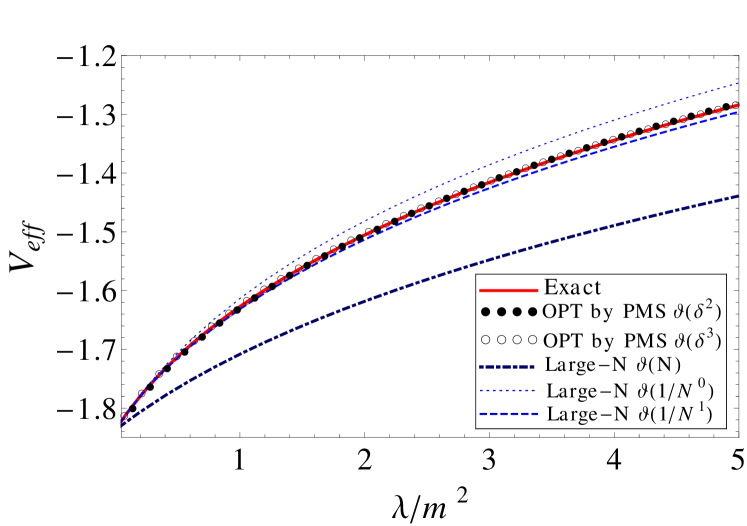
Figure 2: The effective potential $V_{\rm eff}$ for $N=2$. The exact result (solid line), the LN results (dashed-dotted, dotted and dashed lines) and the OPT results (circles), where we optimize $\Sigma$ by using the PMS condition.

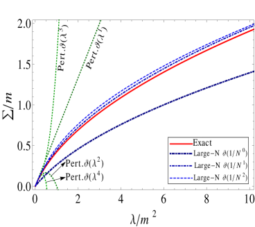
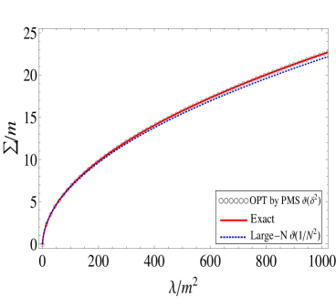
Figure 3: The self-energy $\Sigma$ for $N=2$. Panel (a): The exact result (solid line), LN results (dotted and dashed-dotted lines) and the perturbative results (dotted lines) as a function of the the coupling constant. Panel (b): Extrapolation of the results for the strong coupling regime, for the cases of LN result, shown to $\mathcal{O}(\frac{1}{N^{2}})$ (dashed line), exact result (solid line) and OPT result (circle), shown to $\mathcal{O}(\delta^{2})$ optimizing $\Sigma$ by PMS.

In Fig. 2 we show the results for the effective potential $V_{\rm eff}$ at $N=2$ in the cases of both the OPT and LN. Contrary to the results obtained in perturbation theory and shown in Fig. 1, we see from the results in Fig. 2 that the OPT and LN both produce results with better convergence properties, with the OPT at order $\delta^{2}$ already agreeing quite well with the exact result. This agreement remains even when the coupling is much larger, while the LN results, at increasing orders in $1/N$, tend to oscillate around the exact solution.

Results for self-energy $\Sigma$ at $N=2$ are presented in Fig. 3. In the panel (a) of Fig. 3 we can again see the bad behavior of perturbation theory. In this same panel, we also show the results for the LN for this case, while in the panel (b) of Fig. 3 we show both the LN result at order $1/N^{2}$ and the OPT at analogous order, $\delta^{2}$. Again we see that the OPT covers much better the exact result even for very large values for the coupling constant. Here we have optimized $\Sigma$ by PMS (note that PMS and TP do not present nontrivial solutions at $\mathcal{O}(\delta^{1})$, while the results from FAC are slight worser than the ones obtained with the PMS).

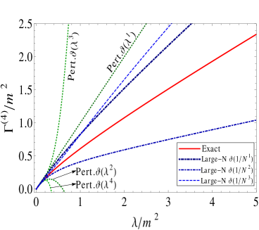
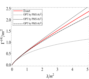
Figure 4: Results for $\Gamma^{(4)}$ for $N=2$. Panel (a): the perturbative results (dotted lines), the LN results (dashed and dashed-dotted lines) and the exact solution (solid line). Panel (b): The exact solution (solid line) and the OPT results shown up to $\mathcal{O}(\delta^{4})$, which were obtained by optimizing $\Sigma$ using the PMS scheme.

Results for $\Gamma^{\left(4\right)}$ are presented in Fig. 4. In the panel (a) of Fig. 4 we show once again the breakdown of perturbation theory, while the LN results present strong deviations from the exact result. In the panel (b) of Fig. 4 we show how by increasing the order in the OPT it oscillates around the exact solution, converging to it. In this case we optimize $\Sigma$ by PMS and use the solution in $\Gamma^{\left(4\right)}$. The other optimization schemes, FAC and TP produce results that are worse. Choosing to optimize the effective potential, or the own function $\Gamma^{\left(4\right)}$ also lead to results that worse than optimizing the self-energy and using the result back in $\Gamma^{\left(4\right)}$. This shows that for this case, optimizing the self-energy as a basic quantity, in the PMS scheme, is the better choice.

In Fig. 5 we verify how the dependence on $N$ influences the results for the effective potential. Three cases are considered, $N=2$, $N=4$ and $N=10$ and both OPT and LN are contrasted with the exact solution. In this case, as we have adopted in Fig. 2, we have chosen to optimize $\Sigma$ using the PMS so to get the optimum solution $\bar{\eta}$ and this solution is then used back in $V_{\rm eff}$. Once again, the PMS applied on the self-energy is found to be the best optimization scheme. The results presented in Fig. 5 also show that in general the OPT presents more robust results than the LN approximation, with the OPT converging faster to the exact result.

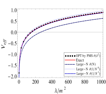
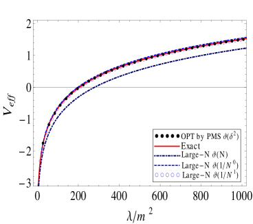
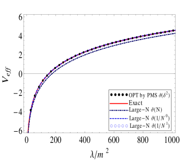
Figure 5: Results for the effective potential $V_{\rm eff}$ for the cases of $N=2$ (panel (a)), $N=4$ (panel (b)) and for $N=10$ (panel (c)). The exact solution is shown with a solid line, the LN results are given by the dashed-dotted, dashed and unfilled circles and the OPT results are represented by filled circles, shown up to $\mathcal{O}(\delta^{2})$. The choice here was to optimize $\Sigma$ using the PMS scheme.

In Figs. 6 and 7 we also study the dependence of the different methods as a function of the number of components $N$, for the fixed value of the parameters in the model, $\lambda/m^{2}=1$, for the self-energy $\Sigma$ and coupling function $\Gamma^{(4)}$, respectively. In Fig. 6, where we show the self-energy $\Sigma$ as a function of $N$, we can see that the LN results tend to present convergence to the exact solution only for very large values of $N$. As in the OPT case, when optimizing the own self-energy $\Sigma$ using the PMS scheme, it shows results that are much weaker dependent on $N$, as far the convergence is concerned. The result from the OPT are also much closer to the exact solution. For comparison purposes, we also show in the panel (b) of Fig. 6 the results obtained using the FAC optimization procedure (applied on $\Sigma$), which also presents a very small deviation from the exact solution, even for larger values of $N$, but it slight under estimates the exact solution when compared with the PMS optimization procedure.

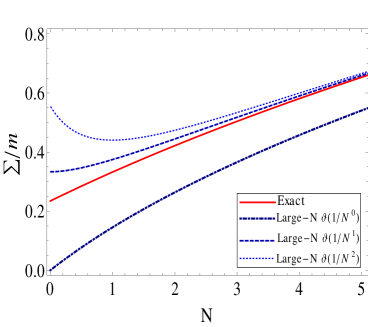
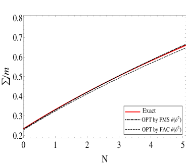
Figure 6: Results for $\Sigma$, for a fixed value of $\frac{\lambda}{m^{2}}=1$, as function of $N$. Panel (a): The exact solution (solid line) and the LN results. panel (b): The exact solution (solid line) and the OPT results to $\mathcal{O}\left(\delta^{2}\right)$ and $\mathcal{O}\left(\delta^{3}\right)$, obtained by optimizing $\Sigma$ by PMS (dotted-dashed) and by FAC (dashed).

Likewise, in Fig. 7 we show the results for $\Gamma^{(4)}$ as a function of $N$ for the different approximation methods. In the panel (a) of Fig. 7 we give the LN results, while in the panel (b) we give the OPT results. We note that LN results present a strong deviation from the exact solution, only tending to converge (in an oscillatory manner) at very larger values of $N$, while the OPT results are robust at any order in $N$ and presents very good with the exact solution already at $\mathcal{O}\left(\delta^{3}\right)$.

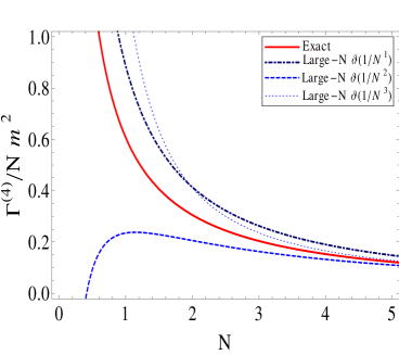
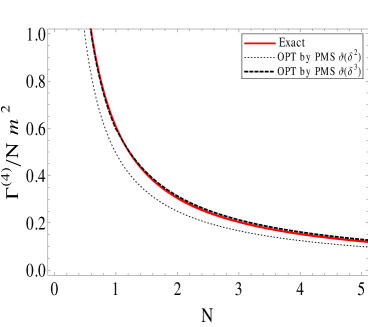
Figure 7: Results for the four point function $\Gamma^{(4)}$, at the fixed value $\frac{\lambda}{m^{2}}=1$, as function of $N$. Panel (a): The exact solution (solid line) and the LN results (dashed, dashed-dotted and dotted lines). Panel (b): The OPT results to $\mathcal{O}\left(\delta^{2}\right)$ and $\mathcal{O}\left(\delta^{3}\right)$, obtained by optimizing $\Sigma$ by PMS.

In Fig. 8 we show how the different optimization schemes within the OPT, the PMS, FAC and TP, affect the result for $V_{\rm eff}$. It is also compared the results by applying those optimization schemes either to the effective potential itself, or to the self-energy and using the produced optimal value of $\eta$ back in the effective potential. These results show that the best agreement with the exact solution is obtained by optimizing $\Sigma$ with PMS. The same is repeated when we evaluate the self-energy $\Sigma$, whose results are shown in Fig. 9, and for the 1PI four point function $\Gamma^{(4)}$, shown in Fig. 10. In all these cases, the best converging results are obtained when we choose to optimize the self-energy in the PMS scheme.

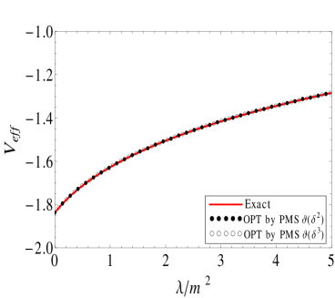
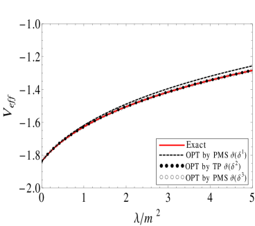
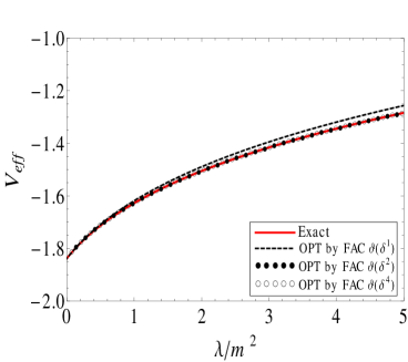
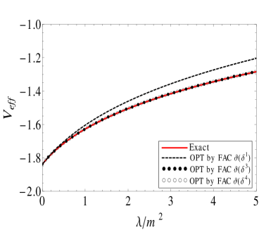
Figure 8: Exact result (solid line) and OPT results (dashed line and circles) for $V_{\rm eff}$ at $N=2$ when we optimize: $\Sigma$ by PMS (panel (a)), $V_{\rm eff}$ by PMS and TP (panel (b)), $\Sigma$ by FAC (panel (c)) and $V_{\rm eff}$ by FAC (panel (d)).

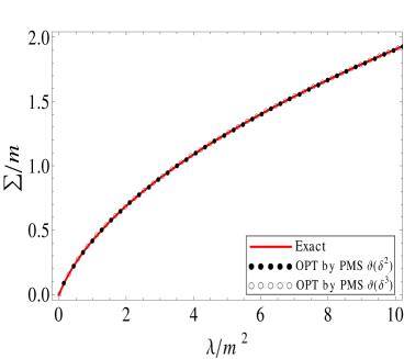
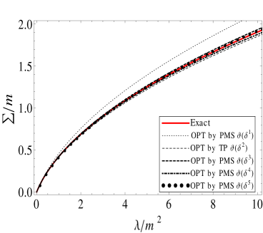
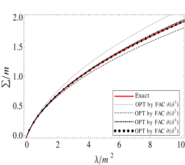
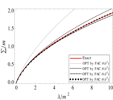
Figure 9: Exact result (solid line) and OPT results for $\Sigma$ at $N=2$ when we optimize: $\Sigma$ by PMS (panel (a)), $V_{\rm eff}$ by PMS and TP (panel (b)), $\Sigma$ by FAC (panel (c)) and $V_{\rm eff}$ by FAC (panel (d)).

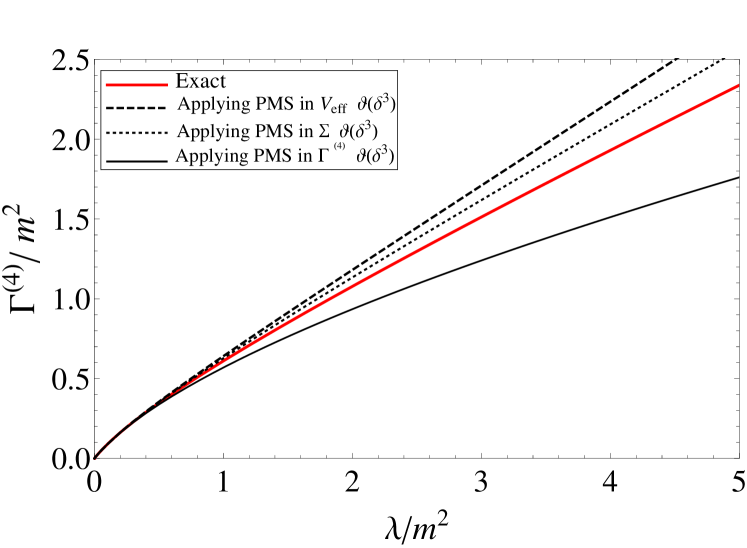
Figure 10: Exact (solid line) and OPT results up to $\mathcal{O}(\delta^{3})$ for the 1PI four point function $\Gamma^{(4)}$ at $N=2$.

Let us better quantify the differences between the two nonperturbative methods studied in this work, the OPT and the LN approximation. We want also to quantify the differences between the different optimization schemes. This is done next, where we analyze the percentage difference that each method produces. We define the percentage difference as

$$\Phi_{\%}=\left|\frac{\Phi_{\rm exact}-\Phi_{\rm approximated}}{\Phi_{\rm exact}}\right|,$$ (28)

where $\Phi$ can represent any physical quantity evaluated in this work: $V_{eff}$, $\Sigma$ or $\Gamma^{(4)}$. In Figs. 11, 12 and 13 we show the percentage difference for $\Sigma$, $V_{\rm eff}$ and $\Gamma^{(4)}$, respectively. Panel (a) in these figures always refers to the OPT results, where, based on the previous results, we have chosen to optimize the self-energy in the two schemes that performs well, the PMS and the FAC schemes. The results shown in panel (b) show the analogous percentage difference of the approximation compared to the exact solution, but for the LN approximation. For convenience, we have chosen two fixed values for $N$, $N=2$ and $N=4$. We can see that the OPT results are quite impressive, showing good convergence in most cases already at second order, while the LN results present strong deviations from the exact solution. In particular, we can see that the OPT provides excellent results for $\Sigma$ and $V_{\rm eff}$, but for $\Gamma^{(4)}$ it is necessary to go to higher orders in $\delta$. As we expected, if we increase the value of $N$ LN presents better results, but still it under performs when compared with the OPT results.

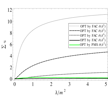
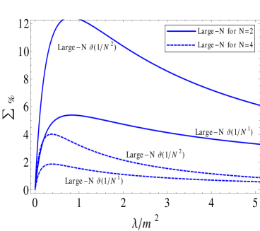
Figure 11: Percentage difference for the $\Sigma$. Panel (a): OPT results for $N=2$ obtained by optimizing $\Sigma$ by FAC (up to $\mathcal{O}(\delta^{5})$) and PMS (up to $\mathcal{O}(\delta^{2})$). Panel (b): LN results for $N=2$ and $N=4$.

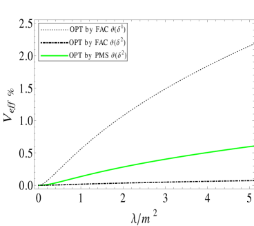
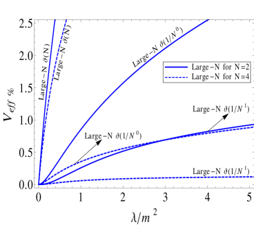
Figure 12: Percentage difference for the $V_{\rm eff}$. Panel (a): OPT results for $N=2$ obtained by optimizing $\Sigma$ by PMS and FAC. Panel (b): LN results for $N=2$ and $N=4$.

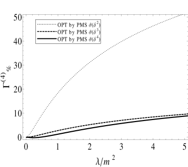
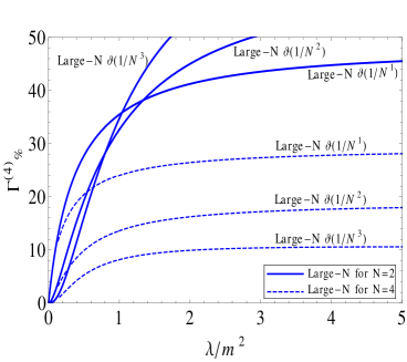
Figure 13: Percentage difference for the $\Gamma^{(4)}$. Panel (a): OPT results for $N=2$ obtained by optimizing $\Sigma$ by PMS. Panel (b): LN results for $N=2$ and $N=4$.

5 Conclusions

In this work we have investigated in details the application of the OPT in the 0-dimensional $O(N)$ scalar field model. The questions we wanted to answer with these work were, which optimization scheme works better with the OPT and which quantity should we optimize to obtain the optimum mass parameter that the OPT makes use to generate nonperturbative results. Through this study, we were able to better access the convergence of the OPT with respect to the different optimization schemes and with respect to each physical quantity that they should be applied (for earlier studies on the convergence of the OPT in the context of the anharmonic potential, see, e.g., Ref. [40], while for a critical theory in field theory, Ref. [42]). Through the results obtained, we have reached the conclusion that the PMS applied to the self-energy is in general be best choice for producing results with better and faster convergence.

One of the main advantages of the OPT method is its easy implementation, that follows in practice the standard perturbative expansion, but still able to generate nonperturbative results when complemented with a proper optimization procedure. In this work, we have better clarified which optimization procedure is the ideal and to which physical quantity it should be applied. For comparative purposes, we have contrasted the results obtained with the OPT method with another popular nonperturbative scheme, the LN expansion. Our results have shown that the OPT is not only competitive but also out performs the results obtained with the LN method. Despite the simplicity of the model we have used in this study, our results indicate that the OPT method can indeed be a better and simpler alternative when applied to theories in physical dimensions $D>0$.

Our results are then expected to better motivate the use of the OPT method as a powerful nonperturbative technique, specially when combined with appropriate optimization schemes (for recent advances on the OPT method and its combination also with renormalization group techniques, see, e.g., Refs. [30, 31, 32]).

6 Acknowledgements

Work partially financed by Conselho Nacional de Desenvolvimento Científico e Tecnológico - CNPq, under the Grant Nos. 475110/2013-7 (R.L.S.F), 232766/2014-2 (R.L.S.F), 308828/2013-5 (R.L.S.F) and 303377/2013-5 (R.O.R.), Fundação Carlos Chagas Filho de Amparo à Pesquisa do Estado do Rio de Janeiro (FAPERJ), under grant No. E - 26 / 201.424/2014 (R.O.R.) and CAPES (D.S.R). R.L.S.F. acknowledges the kind hospitality of the Center for Nuclear Research at Kent State where part of this work has been done.

Appendix A Perturbation Theory

We present here the results obtained when we use perturbation theory to evaluate the Green’s functions for the 0-dimensional $O(N)$ scalar field model. The usual strategy is to expand the interaction term of the partition function in powers of the coupling constant $\lambda$ and then use hyperspherical coordinates to evaluate the generating functional at each order in perturbation theory. For higher orders in the perturbative expansion, we can use the Feynman rules for the model (for futher details, see, e.g., Ref. [36]).

The (non normalized) effective potential $V_{\rm eff}$ for this model can be defined as $V_{\rm eff}=-\ln Z$. The effective potential evaluated in perturbation theory up to $\mathcal{O}\left(\frac{\lambda}{m^{2}}\right)^{6}$ is

$$V_{\rm{eff}} = -\ln\left[\frac{2^{N-1}\pi^{N/2}}{m^{N/2}}\right]+\frac{N^{2}+2N}{24}\left(\frac{\lambda}{m^{2}}\right)-\frac{N^{3}+5N^{2}+6N}{144}\left(\frac{\lambda}{m^{2}}\right)^{2}$$ (29)

$$+ \frac{5N^{4}+44N^{2}+128N^{2}+120N}{2592}\left(\frac{\lambda}{m^{2}}\right)^{3}$$

$$- \frac{7N^{5}+93N^{4}+468N^{3}+1040N^{2}+840N}{10368}\left(\frac{\lambda}{m^{2}}\right)^{4}$$

$$+ \frac{21N^{6}+386N^{5}+2900N^{4}+11000N^{3}+20712N^{2}+15120N}{77760}\left(\frac{\lambda}{m^{2}}\right)^{5}$$

$$- \frac{33N^{7}+793N^{6}+8178N^{5}+45900N^{4}+146000N^{3}+245352N^{2}+166320N}{279936}$$

$$\times \left(\frac{\lambda}{m^{2}}\right)^{6}+\mathcal{O}\left(\left(\frac{\lambda}{m^{2}}\right)^{7}\right).$$

The results for the self-energy $\Sigma$ and $\Gamma^{(4)}$ are, respectively, given by

$$\frac{\Sigma}{m} = \frac{N+2}{6}\left(\frac{\lambda}{m^{2}}\right)^{1}-\frac{N^{2}+6N+8}{36}\left(\frac{\lambda}{m^{2}}\right)^{2}+\frac{N^{3}+11N^{2}+38N+40}{108}\left(\frac{\lambda}{m^{2}}\right)^{3}$$ (30)

$$- \frac{5N^{4}+84N^{3}+512N^{2}+1320N+1184}{1296}\left(\frac{\lambda}{m^{2}}\right)^{4}$$

$$+ \frac{7N^{5}+163N^{4}+1492N^{3}+6640N^{2}+14152N+11296}{3888}\left(\frac{\lambda}{m^{2}}\right)^{5}$$

$$- \frac{21N^{6}+638N^{5}+8020N^{4}+53000N^{3}+192292N^{2}+357680N+261185}{23328}$$

$$\times \left(\frac{\lambda}{m^{2}}\right)^{6}+\mathcal{O}\left(\left(\frac{\lambda}{m^{2}}\right)^{7}\right),$$

and

$$\frac{\Gamma^{\left(4\right)}}{m^{2}} = \left(\frac{\lambda}{m^{2}}\right)^{1}-\frac{N+8}{6}\left(\frac{\lambda}{m^{2}}\right)^{2}+\frac{3N^{2}+46N+140}{36}\left(\frac{\lambda}{m^{2}}\right)^{3}$$ (31)

$$- \frac{5N^{3}+117N^{2}+772N+1536}{108}\left(\frac{\lambda}{m^{2}}\right)^{4}$$

$$+ \frac{35N^{4}+1124N^{3}+11880N^{2}+51568N+79168}{1296}\left(\frac{\lambda}{m^{2}}\right)^{5}$$

$$- \frac{63N^{5}+2609N^{4}+38874N^{3}+271676N^{2}+906576N+1164032}{3888}\left(\frac{\lambda}{m^{2}}\right)^{6}$$

$$+ \mathcal{O}\left(\left(\frac{\lambda}{m^{2}}\right)^{7}\right).$$

Appendix B High order terms in the OPT

In this appendix we present the results obtained for the OPT when expanded up to order $\delta^{(5)}$ for effective potential $V_{\rm eff}$, for the self-energy $\Sigma$ and for the 1PI four-point Green function $\Gamma^{(4)}$. These results are obtained following the perturbative expansion in terms of the parameter $\delta$, using as interaction term Eq. (19). The expressions for $V_{\rm eff}$, $\Sigma$ and $\Gamma^{(4)}$ are given, respectively, by

$$V_{{\rm{eff}}} = -\ln\left[\frac{2^{N-1}\ \pi^{N/2}}{(m+\eta)^{N/2}}\right]\delta^{0}+\frac{\lambda(2N+N^{2})-12N\eta(m+\eta)}{24(m+\eta)^{2}}\delta^{1}$$ (32)

$$+ \frac{-\lambda^{2}(6N+5N^{2}+N^{3})+\lambda\eta(24N+12N^{2})(m+\eta)-\eta^{2}36N(m+\eta)^{2}}{144(m+\eta)^{4}}\delta^{2}$$

$$+ \left[\frac{\lambda^{3}(120N+128N^{2}+44N^{3}+5N^{4})-\lambda^{2}\eta(432+36N^{2}+72N^{3})(m+\eta)}{2592(m+\eta)^{6}}\right.$$

$$+ \left.\frac{\lambda\eta^{2}(648N+324N^{2})(m+\eta)^{2}}{2592(m+\eta)^{6}}-\frac{\eta^{3}N}{6(m+\eta)^{3}}\right]\delta^{3}$$

$$+ \left[\frac{-\lambda^{4}(840N+1040N^{2}+468N^{3}+93N^{4}+7N^{5})}{10368(m+\eta)^{8}}\right.$$

$$+ \left.\frac{\lambda^{3}\eta(120N+128N^{2}+44N^{3}+5N^{4})}{432(m+\eta)^{7}}-\frac{\lambda^{2}\eta^{2}(30N+25N^{2}+5N^{3})}{72(m+\eta)^{6}}\right.$$

$$+ \left.\frac{\lambda\eta^{3}(2N+N^{2})}{6(m+\eta)^{5}}-\frac{\eta^{4}N}{8(m+\eta)^{4}}\right]\delta^{4}$$

$$+ \left[\frac{\lambda^{5}(15120N+20712N^{2}+11000N^{3}+2900N^{4}+386N^{5}+21N^{6})}{77760(m+\eta)^{10}}\right.$$

$$- \left.\frac{\lambda^{4}\eta(840N+1040N^{2}+468N^{3}+93N^{4}+7N^{5})}{1296(m+\eta)^{9}}\right.$$

$$- \left.\frac{\lambda^{2}\eta^{3}(30N+25N^{2}+5N^{3})}{36(m+\eta)^{7}}+\frac{\lambda^{3}\eta^{2}(840N+896N^{2}+308N^{3}+35N^{4})}{864(m+\eta)^{8}}\right.$$

$$+ \left.\frac{\lambda\eta^{4}(10N+5N^{2})}{24(m+\eta)^{6}}-\frac{\eta^{5}N}{10(m+\eta)^{5}}\right]\delta^{5}+\mathcal{O}\left(\delta^{(6)}\right),$$

$$\frac{\Sigma}{m} = \frac{\eta}{m}\delta^{0}+\frac{\lambda(2+N)-6\eta(m+\eta)}{6m(m+\eta)}\delta^{1}$$ (33)

$$- \frac{\lambda^{2}(8+6N+N^{2})-\lambda\eta(12N+6N)(m+\eta)^{2}}{36m(m+\eta)^{3}}\delta^{2}$$

$$+ \frac{\lambda^{3}(40+38N+11N^{2}+N^{3})}{108m(m+\eta)^{5}}\delta^{3}$$

$$- \frac{\lambda^{2}\eta(72+54N+9N^{2})(m+\eta)+\lambda\eta^{2}(36+18N)(m+\eta)^{2}}{108m(m+\eta)^{5}}\delta^{3}$$

$$- \left[\frac{\lambda^{4}(1184+1320N+512N^{2}+84N^{3}+5N^{4})}{1296m(m+\eta)^{7}}\right.$$

$$+ \left.\frac{\lambda^{3}\eta(2400+2280N+660N^{2}+60N^{3})(m+\eta)}{1296m(m+\eta)^{7}}\right.$$

$$+ \left.\frac{\lambda^{2}\eta^{2}(8+6N+N^{2})}{6m(m+\eta)^{5}}-\frac{\lambda\eta^{3}(2+N)}{6m(m+\eta)^{4}}\right]\delta^{4}$$

$$- \left[\frac{\lambda^{5}(11296+14152N+6640N^{2}+1492N^{3}+163N^{4}+7N^{5})}{3888m(m+\eta)^{9}}\right.$$

$$- \left.\frac{\lambda^{4}\eta(8288+9240N+3584N^{2}+588N^{3}+35N^{4})}{1296m(m+\eta)^{8}}\right.$$

$$+ \left.\frac{\lambda^{3}\eta^{2}(200+190N+55N^{2}+5N^{3})}{36m(m+\eta)^{7}}-\frac{\lambda^{2}\eta^{3}(40+30N+5N^{2})}{18m(m+\eta)^{6}}\right.$$

$$+ \left.\frac{\lambda\eta^{4}(2+N)}{6m(m+\eta)^{5}}\right]\delta^{5}+\mathcal{O}\left(\delta^{(6)}\right),$$

and

$$\frac{\Gamma^{\left(4\right)}}{m^{2}} = \frac{\lambda}{m^{2}}\delta^{1}-\frac{\lambda^{2}(8+N)}{6m^{2}(m+\eta)^{2}}\delta^{2}$$ (34)

$$+ \frac{\lambda^{3}(140+46N+3N^{2})-\lambda^{2}\eta(96+12N)(m+\eta)}{36m^{2}(m+\eta)^{4}}\delta^{3}$$

$$- \left[\frac{\lambda^{4}(1536+1772N+117N^{2}+5N^{3})}{108m^{2}(m+\eta)^{6}}-\frac{\lambda^{3}\eta(140+46N+3N^{2})}{9m^{2}(m+\eta)^{5}}\right.$$

$$+ \left.\frac{\lambda^{2}\eta^{2}(8+N)}{2m^{2}(m+\eta)^{4}}\right]\delta^{4}$$

$$+ \left[\frac{\lambda^{5}(79168+51568N+11880N^{2}+1124N^{3}+35N^{4})}{1296m^{2}(m+\eta)^{8}}\right.$$

$$- \left.\frac{\lambda^{4}\eta(1136+772N+1117N^{2}+5N^{3})}{18m^{2}(m+\eta)^{7}}\right.$$

$$+ \left.\frac{\lambda^{3}\eta^{2}(700+230N+15N^{2})}{18m^{2}(m+\eta)^{6}}-\frac{\lambda^{2}\eta^{3}(16+2N)}{3m^{2}(m+\eta)^{5}}\right]\delta^{5}$$

$$+ \mathcal{O}\left(\delta^{(6)}\right).$$

Appendix C Large-$N$ Approximation

The LN approximation applied for the 0-dimensional $O(N)$ scalar field model was described in details in Ref. [36]. In this appendix we reproduce some of the expressions obtained from that reference that we have used in this work. For this model, we have that $\bm{\varphi}^{2}=\mathcal{O}(N)$ and $\lambda=\mathcal{O}(1/N)$, which shows that $\lambda\rightarrow\tilde{\lambda}/N$ is a reasonable replacement. In the large-$N$ limit we can evaluate the partition function $Z$ in the saddle-point approximation [43] (leading and next-to-leading orders terms).

Performing the change of variables $\left(y=\frac{\bm{\varphi}^{2}}{N}\right)$ and using hyperspherical coordinates we can evaluate the partition function that can be written as

$$Z=\Omega_{N}N^{N/2}\int_{0}^{\infty}\frac{dy}{2y}e^{-Nf(y)},$$ (35)

where the function $f(y)$ is defined by

$$f(y)=\frac{m}{2}y+\frac{\tilde{\lambda}}{4!}y^{2}-\frac{1}{2}\ln(y).$$ (36)

In a saddle point approximation we perform an expansion in Eq. (36) around its minimum,

$$y_{0}=\frac{3m}{\tilde{\lambda}}\left(\sqrt{1+\frac{2\tilde{\lambda}}{3m^{2}}}-1\right).$$ (37)

Expanding around this minimum and performing the integral, we obtain the partition function [36]

$$Z = \Omega_{N}N^{\frac{N}{2}}e^{-Nf\left(y_{0}\right)}\left(\frac{1}{4y_{0}^{2}}\frac{2\pi}{f^{\prime\prime}\left(y_{0}\right)}\right)^{1/2}$$ (38)

$$\times \left[1+\frac{12m^{2}y_{0}^{2}-27my_{0}+16}{6N(2-my_{0})^{3}}\right]\left[1+\mathcal{O}(1/N)\right],$$

with

$$f(y_{0})=\frac{my_{0}}{4}+\frac{1}{4}-\frac{1}{2}\ln(y_{0}).$$ (39)

Next-to-leading order LN results for $\Gamma^{(0)}$ can be obtained by taking the logarithm of $\frac{Z}{Z_{0}}$:

$$\Gamma^{(0)} = \left[\frac{my_{0}}{4}-\frac{1}{4}-\frac{1}{2}\ln(my_{0})\right]N^{1}+\frac{1}{2}\ln(2-my_{0})N^{0}$$ (40)

$$- \frac{(8+my_{0})(my_{0}-1)^{2}}{6(2-my_{0})^{3}}\frac{1}{N^{1}}$$

$$+ \mathcal{O}(1/N^{2}).$$

Higher order terms in $1/N$ usually are very difficult to obtain because we need go beyond the saddle-point approximation, including fluctuations in the corrections. But for the case of the 0-dimensional $O(N)$ scalar field model, it can be obtained by successive derivatives of $\Gamma^{(0)}$ with respect to $m$. Following this procedure, we can for the self-energy the result

$$\Sigma = \left[\frac{1}{y_{0}}-m\right]\frac{1}{N^{0}}+\left[\frac{2(1-my_{0})}{y_{0}(2-my_{0})^{2}}\right]\frac{1}{N^{1}}$$ (41)

$$+ \left[\frac{4(my_{0}-1)^{2}(3my_{0}-1)}{y_{0}(2-my_{0})^{5}}\right]\frac{1}{N^{2}}$$

$$+ \mathcal{O}(1/N^{3}),$$

and also for the 1PI four-point function,

$$\Gamma^{(4)} = \left[\frac{6(1-my_{0})}{y_{0}^{2}(2-my_{0})}\right]\frac{1}{N}$$ (42)

$$- \left[\frac{12(1-my_{0})^{2}(m^{2}y_{0}^{2}-3my_{0}+6)}{y_{0}^{2}(2-my_{0})^{4}}\right]\frac{1}{N^{2}}$$

$$+ \left[\frac{24(1-my_{0})^{3}}{y_{0}^{2}(2-my_{0})^{7}}\right.$$

$$\times \left.(m^{4}y_{0}^{4}-8m^{3}y_{0}^{3}+35m^{2}y_{0}^{2}-49my_{0}+56)\right]\frac{1}{N^{3}}$$

$$+ \mathcal{O}(1/N^{4}).$$

Appendix D The optimum $\eta$

We give below the expressions for the optimum $\eta$ obtained in each of the optimization procedures that we have explained in the text, when applied to the different physical quantities, i.e., to the self-energy, the effective potential and to the four-point Green’s function.

1. $\bar{\eta}$ obtained by optimizing the self-energy $\Sigma$:

   • using PMS:

     $$\bar{\eta} = \frac{m}{2}\left(-1+\sqrt{1+(4+N)\frac{\lambda}{m^{2}}}\right)\delta^{2}+\frac{m}{6}\biggl{(}-3$$ (43)

     $$+ \sqrt{9+12(4+N)\frac{\lambda}{m^{2}}-2\sqrt{6\left(-4+3N+N^{2}\right)\frac{\lambda^{2}}{m^{4}}}}\biggr{)}$$

     $$\times \delta^{3}+\mathcal{O}\left(\delta^{4}\right).$$

     Note that there is no solution (real and positive) for $\bar{\eta}$ at order $\delta^{1}$.

   • using FAC:

     $$\bar{\eta} = \frac{m}{6}\left(-3+\sqrt{9+6(2+N)\frac{\lambda}{m^{2}}}\right)\delta^{1}$$ (44)

     $$+ \frac{m}{6}\left(-3+\sqrt{9+6(4+N)\frac{\lambda}{m^{2}}}\right)\delta^{2}$$

     $$+ \frac{m}{6}\left(-3+\sqrt{9+9(4+N)\frac{\lambda}{m^{2}}-3\sqrt{\left(N^{2}-16\right)\frac{\lambda^{2}}{m^{4}}}}\right)\delta^{3}$$

     $$+ \mathcal{O}\left(\delta^{4}\right).$$

     Note that for $N<4$ there is no solution (real and positive) for $\bar{\eta}$ at order $\delta^{3}$.

   • using TP:

     $$\bar{\eta} = \frac{m}{4}\left(-1+\sqrt{9+8(4+N)\frac{\lambda}{m^{2}}}\right)\delta^{2}+\frac{1}{12}\Biggl{\{}\sqrt{F}-3m$$ (45)

     $$- \left[\frac{432B-\left(\sqrt{F}-3m\right)\left(-24A+F+3\sqrt{F}m-18m^{2}\right)}{\sqrt{F}}\right]^{\frac{1}{2}}\Biggr{\}}$$

     $$\times \delta^{3}+\mathcal{O}\left(\delta^{4}\right),$$

     where we have defined

     $$A = 3m^{2}+4\lambda(4+N),$$ (46)

     $$B = m^{3}+m\lambda(4+N),$$ (47)

     $$C = (4+N)\left[6m^{2}\lambda+5\lambda^{2}(5+N)\right],$$ (48)

     $$D = 36m^{4}+(4+N)\left[87m^{2}\lambda+2\lambda^{2}(107+23N)\right],$$ (49)

     $$E = -4A^{3}+1458B^{2}+72AC-162ABm+81Cm^{2},$$ (50)

     $$+ \biggl{\{}-16D^{3}+\biggl{[}-4A^{3}+18A(4C-9Bm)+81\biggl{(}18B^{2}$$

     $$+ Cm^{2}\biggr{)}\biggr{]}^{2}\biggr{\}}^{\frac{1}{2}},$$

     $$F = 8A+\frac{2^{8/3}D}{E^{1/3}}+2^{4/3}E^{1/3}+9m^{2}.$$ (51)

     Note that in this case there is no solution (real and positive) for $\bar{\eta}$ at order $\delta^{1}$.

2. $\bar{\eta}$ optimizing the effective potential $V_{\rm{eff}}$

   • using PMS:

     $$\bar{\eta} = \frac{m}{6}\left(-3+\sqrt{9+(12+6N)\frac{\lambda}{m^{2}}}\right)\delta^{1}+\frac{m}{6}\Biggl{(}\frac{}{}-3$$ (52)

     $$+ \sqrt{9+(18+9N)\frac{\lambda^{2}}{m^{4}}-3\sqrt{\left(-12-4N+N^{2}\right)\frac{\lambda^{2}}{m^{4}}}}\Biggr{)}\delta^{2}$$

     $$+ \frac{1}{6G^{1/3}}\left(-3G^{1/3}m+G^{\prime}\right)\delta^{3}+\mathcal{O}\left(\delta^{4}\right),$$

     where we have defined the constants

     $$G = 9\left(8+N^{3}\right)\lambda^{3}+\biggl{[}-3(2+N)^{2}\biggl{(}-2160+1296N-36N^{2},$$ (53)

     $$- 116N^{3}+5N^{4}\biggr{)}\lambda^{6}\biggr{]}^{\frac{1}{2}},$$

     and

     $$G^{\prime} = \biggl{[}2^{2/3}3^{1/3}G+2^{7/3}3^{2/3}G^{1/3}\left(-6-N+N^{2}\right)\lambda^{2},$$ (54)

     $$+ G^{2/3}\left(9m^{2}+(24+12N)\lambda\right)\biggr{]}^{\frac{1}{2}}.$$

     Note that in this case, for $N<6$ there is no solution (real and positive) for $\bar{\eta}$ at order $\delta^{2}$.

   • using FAC:

     $$\bar{\eta} = \frac{m}{6}\left(-3+\sqrt{9+3(2+N)\frac{\lambda}{m^{2}}}\right)\delta^{1}$$ (55)

     $$+ \frac{1}{6H^{1/3}}\left(-3H^{1/3}m+H^{\prime}\right)\delta^{3}+\mathcal{O}\left(\delta^{4}\right),$$

     where we have defined the additional constants

     $$H = \left(24+4N-2N^{2}+N^{3}\right)\lambda^{3},$$ (56)

     $$+ \sqrt{8(2+N)^{2}\left(72-12N-4N^{2}+N^{3}\right)\lambda^{6}},$$

     and

     $$H^{\prime} = \biggl{[}3I+H^{1/3}\left(-12-4N+N^{2}\right)3\lambda^{2}$$ (57)

     $$+ 9H^{2/3}m^{2}\left(1+(2+N)\frac{\lambda}{m^{2}}\right)\biggr{]}^{\frac{1}{2}}.$$

     Here there is no solution (real and positive) for $\bar{\eta}$ at order $\delta^{2}$.

   • using TP:

     $$\bar{\eta} = \frac{m}{\sqrt{2}}\left(\sqrt{2+(2+N)\frac{\lambda}{m^{2}}}\right)\delta^{1}$$ (58)

     $$+ \left(-\frac{1}{2}\sqrt{2I+\frac{6\sqrt{6}J}{\sqrt{54I+\frac{27L}{O^{1/3}}+O^{1/3}}}-\frac{L}{2O^{1/3}}-\frac{O^{1/3}}{54}}\right.$$

     $$+ \left.\frac{\sqrt{54I+\frac{27L}{O^{1/3}}+O^{1/3}}}{6\sqrt{6}}\right)\delta^{2}+\mathcal{O}\left(\delta^{3}\right),$$

     where

     $$I = 2m^{2}+\lambda(2+N),$$ (59)

     $$J = 2m^{3}+m\lambda(2+N),$$ (60)

     $$K = -(2+N)\biggl{[}9m^{2}\lambda+5\lambda^{2}(3+N)\biggr{]},$$ (61)

     $$L = 108m^{4}+(2+N)\biggl{[}180m^{2}\lambda$$ (62)

     $$+ \lambda^{2}(174+67N)\biggr{]},$$

     $$M = 2916m^{4}+27(2+N)\biggl{[}180m^{2}\lambda$$ (63)

     $$+ \lambda^{2}(174+67N)\biggr{]},$$

     $$O = -19683I^{3}+78732J^{2}-17496IK$$ (64)

     $$- \sqrt{4782969\left(9I^{3}-36J^{2}+8IK\right)^{2}-M^{3}}.$$

3. $\bar{\eta}$ optimizing the $\Gamma^{(4)}$

   • using PMS:

     $$\bar{\eta} = \frac{m}{18(8+N)}\biggl{\{}-9(8+N)+\biggl{[}9(8+N)\biggl{(}9(8+N)$$ (65)

     $$+ 4\left(140+46N+N^{2}\right)\frac{\lambda}{m^{2}}\biggr{)}\biggr{]}^{\frac{1}{2}}\biggr{\}}\delta^{3}+\mathcal{O}\left(\delta^{4}\right).$$

   • using FAC:

     $$\bar{\eta} = \frac{m}{24(8+N)}\biggl{\{}-12(8+N)+\biggl{[}48(8+N)\biggl{(}3(8+N)$$ (66)

     $$+ \left(140+46N+3N^{2}\right)\frac{\lambda}{m^{2}}\biggr{)}\biggr{]}^{\frac{1}{2}}\biggr{\}}\delta^{3}+\mathcal{O}\left(\delta^{4}\right).$$

   • using TP:

     $$\bar{\eta} = \frac{m}{9(8+N)}\biggl{\{}-3(8+N)+\biggl{[}3(8+N)\biggl{(}12(8+N)$$ (67)

     $$+ 5(140+46N+3N^{2})\frac{\lambda}{m^{2}}\biggr{)}\biggr{]}^{\frac{1}{2}}\biggr{\}}\delta^{3}+\mathcal{O}\left(\delta^{4}\right),$$

   Note that there is no solution (real and positive) for $\bar{\eta}$ at orders $\delta^{1}$ and $\delta^{2}$ for the three optimization procedures applied to $\Gamma^{(4)}$.

References

- [1] D. J. Gross, R. D. Pisarski and L. G. Yaffe,“QCD and Instantons at Finite Temperature,” Rev. Mod. Phys. 53 (1981) 43. doi:10.1103/RevModPhys.53.43
- [2] J. R. Espinosa, M. Quiros and F. Zwirner, “On the phase transition in the scalar theory,” Phys. Lett. B 291 (1992) 115 doi:10.1016/0370-2693(92)90129-R [hep-ph/9206227].
- [3] M. Gleiser and R. O. Ramos, “Thermal fluctuations and validity of the one loop effective potential,” Phys. Lett. B 300 (1993) 271 doi:10.1016/0370-2693(93)90365-O [hep-ph/9211219].
- [4] M. Moshe and J. Zinn-Justin,“Quantum field theory in the large N limit: A Review,” P hys. Rept. 385 (2003) 69 doi:10.1016/S0370-1573(03)00263-1 [hep-th/0306133].
- [5] A. Okopinska, “Nonstandard Expansion Techniques For The Effective Potential In Lambda Phi**4 Quantum Field Theory,” Phys. Rev. D 35 (1987) 1835. doi:10.1103/PhysRevD.35.1835
- [6] S. Gandhi and M. B. Pinto, “ expansion of models with chiral-symmetry breaking”, Phys. Rev. D 46, (1992) 2570.
- [7] H. Yamada, “Spontaneous symmetry breaking in QCD”, Z. Phys. C 59, (1993) 67.
- [8] K. G. Klimenko, “Nonlinear optimized expansions and the Gross-Neveu model”, Z. Phys. C 60, (1993) 677.
- [9] J.-L. Kneur, M. B. Pinto and R. O. Ramos,“Asymptotically improved convergence of optimized perturbation theory in the Bose-Einstein condensation problem”, Phys. Rev. A 68, (2003) 043615.
- [10] M. B. Pinto, R. O. Ramos, and P. J. Sena,“Evaluating Critical Exponents in the Optimized Perturbation Theory”, Phys. A 342 (2004) 570.
- [11] R. L. S. Farias, G. Krein and R. O. Ramos, “Applicability of the linear expansion for the field theory at finite temperature in the symmetric and broken phases”, Phys. Rev. D 78, (2008) 065046.
- [12] R. L. S. Farias, D. L. Teixeira Jr. and R. O. Ramos, “Reliability of the Optimized Perturbation Theory for scalar fields at finite temperature”, AIP Conf. Proc. 1520, (2013) 330; D. C. Duarte, R. L. S. Farias and R. O. Ramos, “Non-perturbative description of self-interacting charged scalar field at finite temperature and in the presence of an external magnetic field”, AIP Conf. Proc. 1520, (2013) 349; R. L. S. Farias, D. L. Teixeira Jr. and R. O. Ramos, “Bulk viscosity in optimized perturbation theory”, AIP Conf. Proc. 1296, (2010) 406.
- [13] M. C. B. Abdalla, J. A. Helayel-Neto, D.L. Nedel, and C.R. Senise, Jr., “An extension of the linear delta expansion to superspace”, Phys. Rev. D 77, (2008) 125020.
- [14] D. C. Duarte, R. L. S. Farias and R. O. Ramos,“Optimized perturbation theory for charged scalar fields at finite temperature and in an external magnetic field”, Phys. Rev. D 84, (2011) 083525.
- [15] M.C.B. Abdalla, R.L.S. Farias, J.A. Helayel-Neto, D.L. Nedel, C.R. Senise, Jr, “Supergraph approach in a higher-order linear delta expansion calculation of the effective potential for F-type broken supersymmetry”, Phys. Rev. D 86, (2012) 085024.
- [16] S. Chiku and T. Hatsuda, “Optimized perturbation theory at finite temperature”, Phys. Rev. D 58, (1998) 076001.
- [17] S. Chiku, “Optimized perturbation theory at finite temperature: Two loop analysis”, Prog. Theor. Phys. 104, (2000) 1129;
- [18] E. Braaten and E. Radescu, “Convergence of the Linear Expansion in the Critical O(N) Field Theory”, Phys. Rev. Lett. 89, (2002) 271602.
- [19] H. Kleinert and W. Janke, “Convergence behavior of variational perturbation expansion - A method for locating Bender-Wu singularities”, Phys. Lett. A 206, (1995) 283; H. Kleinert, “Strong-coupling behavior of theories and critical exponents”, Phys. Rev. D 57, (1998) 2264; R. P. Feynman and H. Kleinert, “Effective classical partition functions”, Phys. Rev. A 34, (1986) 5080.
- [20] V.I. Yukalov, “Theory of perturbations with a strong interaction.”, Moscow Univ. Phys. Bull. 31, (1976) 10; “Model of a hybrid crystal”, Theor. Math. Phys. 28, (1976) 652; V. I. Yukalov and E. P. Yukalova,“Self-similar perturbation theory”, Ann. Phys. 277, (1999) 219; “Self-Similar Structures and Fractal Transforms in Approximation Theory”, Chaos Solitons Fractals 14, (2002) 839.
- [21] I. R. C. Buckley, A. Duncan and H. F. Jones, “Proof of the convergence of the linear expansion: Zero dimensions”, Phys. Rev. D 47, 2554 (1993); C. M. Bender, A. Duncan and H. F. Jones, “Convergence of the optimized expansion for the connected vacuum amplitude: Zero dimensions”, Phys. Rev. D 49, (1994) 4219; C. Arvanitis, H. F. Jones and C. S. Parker, “Convergence of the optimized expansion for the connected vacuum amplitude: Anharmonic oscillator”, Phys. Rev. D 52, (1995) 3704.
- [22] J.O. Andersen, E. Braaten and M. Strickland, “Screened perturbation theory to three loops”, Phys. Rev. D 63, (2001) 105008.
- [23] E. Braaten and R. D. Pisarski, Phys. Rev. D 45 (1992) 1827. doi:10.1103/PhysRevD.45.R1827
- [24] J. O. Andersen and M. Strickland, Annals Phys. 317 (2005) 281 doi:10.1016/j.aop.2004.09.017 [hep-ph/0404164].
- [25] P. M. Stevenson, “Optimized Perturbation Theory,” Phys. Rev. D 23 (1981) 2916. doi:10.1103/PhysRevD.23.2916
- [26] G. Krein, D. P. Menezes and M. B. Pinto, “Optimized delta expansion for the Walecka model,” Phys. Lett. B 370 (1996) 5 doi:10.1016/0370-2693(95)01578-7 [nucl-th/9510059].
- [27] J. L. Kneur, M. B. Pinto and R. O. Ramos, “Critical and tricritical points for the massless 2D Gross-Neveu model beyond large N,” Phys. Rev. D 74 (2006) 125020 doi:10.1103/PhysRevD.74.125020 [hep-th/0610201]. J. L. Kneur, M. B. Pinto, R. O. Ramos and E. Staudt, “Updating the phase diagram of the Gross-Neveu model in 2+1 dimensions,” Phys. Lett. B 657 (2007) 136 doi:10.1016/j.physletb.2007.10.013 [arXiv:0705.0673 [hep-ph]]. J. L. Kneur, M. B. Pinto and R. O. Ramos, “Thermodynamics and Phase Structure of the Two-Flavor Nambu–Jona-Lasinio Model Beyond Large-Nc,” Phys. Rev. C 81 (2010) 065205 doi:10.1103/PhysRevC.81.065205 [arXiv:1004.3815 [hep-ph]].
- [28] M. B. Pinto and R. O. Ramos, “High temperature resummation in the linear delta expansion,” Phys. Rev. D 60 (1999) 105005 doi:10.1103/PhysRevD.60.105005 [hep-ph/9903353].
- [29] M. B. Pinto and R. O. Ramos, “A Nonperturbative study of inverse symmetry breaking at high temperatures,” Phys. Rev. D 61 (2000) 125016 doi:10.1103/PhysRevD.61.125016 [hep-ph/9912273].
- [30] J. L. Kneur and A. Neveu, “ from and Renormalization Group Optimized Perturbation Theory,” Phys. Rev. D 88 (2013) 074025 doi:10.1103/PhysRevD.88.074025 [arXiv:1305.6910 [hep-ph]].
- [31] J.-L. Kneur and M. B. Pinto, “Renormalization Group Optimized Perturbation Theory at Finite Temperatures,” Phys. Rev. D 92 (2015) 116008 doi:10.1103/PhysRevD.92.116008 [arXiv:1508.02610 [hep-ph]].
- [32] J.-L. Kneur and M. B. Pinto, “Scale Invariant Resummed Perturbation at Finite Temperatures,” Phys. Rev. Lett. 116 (2016) 031601 doi:10.1103/PhysRevLett.116.031601 [arXiv:1507.03508 [hep-ph]].
- [33] J. L. Kneur, M. B. Pinto and R. O. Ramos, “Thermodynamics and Phase Structure of the Two-Flavor Nambu–Jona-Lasinio Model Beyond Large-,” Phys. Rev. C 81 (2010) 065205 doi:10.1103/PhysRevC.81.065205 [arXiv:1004.3815 [hep-ph]].
- [34] J. L. Kneur, M. B. Pinto, R. O. Ramos and E. Staudt, “Vector-like contributions from Optimized Perturbation in the Abelian Nambu–Jona-Lasinio model for cold and dense quark matter,” Int. J. Mod. Phys. E 21 (2012) 1250017 doi:10.1142/S0218301312500176 [arXiv:1201.2860 [nucl-th]].
- [35] P. Ramond, Field Theory: A Modern Primer (Addison-Wesely, 1990).
- [36] J. Keitel and L. Bartosch, “The Zero-dimensional O(N) vector model as a benchmark for perturbation theory, the large-N expansion and the functional renormalization group,” J. Phys. A 45 (2012) 105401 doi:10.1088/1751-8113/45/10/105401 [arXiv:1109.3013 [cond-mat.stat-mech]].
- [37] G. Huber, “Gamma function derivation of n-sphere volumes”, A. Math. Mon. 89, (1982) 301.
- [38] Handbook of Mathematical Functions, edited by M. Abramowitz and I. A. Steigen (Dover, New York, 1972), 9th ed.
- [39] H. Kleinert, V. Schulte-Frohlinde, Critical Properties of -Theories, 1th Edition (World scientific Pub Co Inc, Singapore, 2001).
- [40] B. Bellet, P. Garcia and A. Neveu,“Convergent sequences of perturbative approximations for the anharmonic oscillator. 1. Harmonic approach”, Int. J. Mod. Phys. A 11, 5587 (1996); “Convergent sequences of perturbative approximations for the anharmonic oscillator. 2. Compact time approach”, Int. J. Mod. Phys. A 11, (1996) 5607;
- [41] H. Kleinert and V. I. Yukalov, “Self-similar variational perturbation theory for critical exponents”, Phys. Rev. E 71, (2005) 026131.
- [42] J. L. Kneur, M. B. Pinto and R. O. Ramos, “Convergent resummed linear delta expansion in the critical (3-d) model,” Phys. Rev. Lett. 89 (2002) 210403 doi:10.1103/PhysRevLett.89.210403 [cond-mat/0207089].
- [43] G. B. Arfken and H. J. Weber, Mathematical Methods for Physicists, 6th edition (Academic Press, New York, 2005).