Social contagions on weighted networks

Abstract

We investigate critical behaviors of a social contagion model on weighted networks. An edge-weight compartmental approach is applied to analyze the weighted social contagion on strongly heterogenous networks with skewed degree and weight distributions. We find that degree heterogeneity can not only alter the nature of contagion transition from discontinuous to continuous but also can enhance or hamper the size of adoption, depending on the unit transmission probability. We also show that, the heterogeneity of weight distribution always hinder social contagions, and does not alter the transition type.

I Introduction

Network provides a useful analytical framework for studying a wide array of social phenomena, since the network of people—social networks—plays a critical role in many social phenomena Newman (2003); Pastor-Satorras et al. (2015); Castellano et al. (2009); Boccaletti et al. (2006); Cohen and Havlin (2010); Barabási (2015). Although the edges in social networks—social relationships—are often modeled binary, it is more realistic to consider weighted edges because the strength of social relationship greatly vary in reality Barrat et al. (2004). A number of proxies has been used to capture the strength of social relationships. For example, the number of papers that two scientists have coauthored was used to capture the strength of the collaboration Newman (2001); Barrat et al. (2004); the duration of calls—the amount of conversation—between two people is used to measure how close they are Onnela et al. (2007). Thus it is important to ask how the distribution of weights, along with degree distribution, affects various dynamics on networks.

Spreading processes, such as epidemic spreading Pastor-Satorras et al. (2015); Newman (2010); Easley and Kleinberg (2010), diffusion of innovations Rogers (2003); Goffman and Newill (1964); Krapivsky et al. (2011), and diffusion of rumors Moreno et al. (2004); Daley and Kendall (1964); Cheng et al. (2013), are fundamental dynamics on social networks. Recent studies have shown that there exist two important classes of contagions: simple and complex. Simple contagions (e.g. epidemic models such as SIS model Pastor-Satorras and Vespignani (2001) and SIR model Moreno et al. (2002)) refers the processes where contagions spread independently, while complex contagions (e.g. linear threshold model Granovetter (1978); Watts (2002)) refers the processes that are affected by social reinforcement, where more exposures can drastically increase the adoption probability Watts (2002); Centola (2010); Backstrom et al. (2006); Krapivsky et al. (2011).

Previous studies focused mainly on simple contagions, have revealed that strong heterogeneity in the degree and weight distributions not only is ubiquitous Albert and Barabási (2002); Barrat et al. (2004); Pastor-Satorras et al. (2015), but also fundamentally affect the nature of spreading phenomena Pastor-Satorras and Vespignani (2001); Newman (2003); Wang et al. (2014); Gross and Blasius (2008); Holme and Saramäki (2012). For instance, on infinite scale-free networks where the degree distribution exhibits a power-law ($P(k)\sim k^{-\alpha},2<\alpha\leq 3$), the epidemic threshold vanishes Pastor-Satorras and Vespignani (2001); Boguñá et al. (2013). The inhomogeneity of weight distribution can also significantly affect the epidemic threshold, epidemic prevalence, and spreading velocity Wang et al. (2014); Kamp et al. (2013); Rattana et al. (2013); Yan et al. (2005); Yang and Zhou (2012). Although many interesting properties of complex contagion has been uncovered recently Centola (2010); Gleeson (2008); Weng et al. (2013); Nematzadeh et al. (2014), it is not fully understood how degree and weight heterogeneity affect the dynamics of complex contagions. Building on recent progress in complex contagion Dodds and Watts (2004); Schelling (1971); Watts (2002); Krapivsky et al. (2011), here we introduce a weighted complex contagion model and investigate the effect of degree and weight heterogeneity on the dynamics of complex contagion.

We find that (i) increasing heterogeneity of degree distribution changes the nature of the phase transition from discontinuous to continuous; (ii) degree heterogeneity plays opposite roles depends on the unit transmission probability: it enhance the spreading when the unit transmission probability is small while hinder the spreading when the unit transmission probability is large; and (iii) the weight heterogeneity suppress the contagion while not altering the transition type. To analyze the dynamics of complex contagion on weighted networks, we use an edge-weight compartmental approach, which provides accurate results.

II Weighted Complex Contagion Model and Network

We first introduce a complex contagion model that takes weighted edges into account. Our model builds on a simple, generalized non-Markovian contagion model that can describe both simple and complex contagions Krapivsky et al. (2011); Wang et al. (2015a, b). In particular, an individual can be in one of three possible states: susceptible (S), adopted (A), or recovered (R). Each individual has a state of awareness value $m\in[0,T]$ which denotes the number of exposures. An individual adopts and begins to transmit the behavior or information (contagion) when its awareness value reaches $T$. Individuals with $m<T$ do not affect the others. Here we add a weight-based transmission rule—individuals transmit the contagion preferably to its closer neighbors with the following probability:

$$\lambda_{w_{i,j}}=1-(1-\beta)^{w_{i,j}},$$ (1)

where $w_{i,j}$ is the weight of the connection between individual $i$ and $j$, and $\beta$ is the unit transmission probability. Given $\beta$, $\lambda_{w_{i,j}}$ monotonically increases with $w_{i,j}$, i.e., individuals are more likely to transmit the contagion to more strongly connected neighbors. When successful, the awareness value of the neighbor will increase by one. Assume an edge that has transmitted the contagion successfully will never transmit the same information again. Also, each adopted individual may become recovered with probability $\gamma$, considering the fact that people may lose interest in the contagion after a while and will not spread it any more (in this paper, we set $\gamma=1$ unless noted, so everyone is active for only one step). The individuals will remain in recovered state for all subsequent times once it is recovered.

In our networks, we initially select a small fraction of nodes randomly and designate them as seeds by setting their awareness to be $T$. We set the awareness of the remaining nodes to be $0$ and let them be at the susceptible state. In each step, all adopted nodes will interact with all of its susceptible neighbors and transmit the contagion to them with the probability defined above. At the same time, all adopted nodes will recover with certain probability. The spreading process stops when there is no adopted nodes, the final adoption size is equal to final density of recovered nodes.

For simplicity, we assume uncorrelated random graphs specified by two distributions: degree and weight. We realize such networks by generalizing the configuration model Catanzaro et al. (2005); Wang et al. (2014). Consider one network with $N$ nodes and $M$ edges. We first create a graph using the classical configuration model, where the degree distribution follows $p(k)\sim k^{-\alpha_{k}}$ ($3\leq k_{i}\leq\sqrt{N}$), then distribute weights that are sampled from $g(w)\sim w^{-\alpha_{w}}$ randomly ($w_{max}\sim N^{\frac{1}{\alpha_{w}-1}}$). $\alpha_{k}$ ($\alpha_{w}$) controls the heterogeneity of the degree (weight) distribution. Following previous studies Yang and Zhou (2012); Wang et al. (2014), we assume integer weight values as it makes our approach more tractable.

III Theoretical Approach and Numerical Simulation

III.1 Edge-weight compartmental approach

One of the most widely used approaches to study network dynamics—heterogeneous mean-field theory (HMF) Moreno et al. (2002); Castellano and Pastor-Satorras (2006)—separates nodes into each degree bucket while treating all edges equally. While it provides an excellent way to handle strong degree heterogeneity, it overlooks edge weight heterogeneity. As a result, the approach exhibits a limitation in dealing with networks with strong weight heterogeneity Buono et al. (2013). Our edge-weight compartmental approach treat each (integer) weight values separately and provides a better way to study networks with strong weight heterogeneity Volz (2008); Volz et al. (2011); Wang et al. (2014, 2015c).

We use variables $S(t)$, $A(t)$ and $R(t)$ to denote densities of the susceptible, adopted, and recovered nodes at time $t$. Let us consider a randomly selected susceptible node $u$ with awareness value $m$. Node $u$ will remain susceptible as long as $m<T$ and will become adopted once $T$ of its neighbors have transmitted the contagion successfully to $u$ since multiple transmission through an edge is forbidden. As edge weights are assigned randomly, the probability that $u$ is not informed by a neighbor $v$ by time $t$ can be denoted by

$$\theta(t)=\sum_{w}g(w)\theta_{w}(t),$$ (2)

where $\theta_{w}(t)$ denotes the probability that $u$ is not informed by an edge with weight $w$ by time $t$. If $u$’s degree is $k$, the probability that the node was not one of the seeds and received the contagion for $m$ times by time $t$ is

$$\phi_{m}(k,t)=(1-\rho_{0})\binom{k}{m}[\theta(t)]^{k-m}[1-\theta(t)]^{m},$$ (3)

where $A_{0}$ denotes the fraction of seeds. Clearly, the probability that the $k$-degree node was not one of the seeds and still didn’t adopt the contagion by time $t$ is

$$\phi(k,t)=\sum_{m=0}^{T-1}\phi_{m}(k,t).$$ (4)

Thus the fraction of susceptible nodes (the probability that a randomly selected node is susceptible) at time $t$ is

$$S(t)=\sum_{k=0}p(k)\phi(k,t).$$ (5)

Now, let us examine $\theta_{w}(t)$ in Eq.(2), $\theta_{w}(t)$ can be broken down into:

$$\theta_{w}(t)=\xi_{w}^{S}(t)+\xi_{w}^{A}(t)+\xi_{w}^{R}(t),$$ (6)

where $\xi_{w}^{X}(t)$ denote the probability that a neighbor in the state $X\in\{$S,A,R$\}$ has not transmitted the contagion to $u$ through an edge with weight $w$ by time $t$. Once we derive $\xi_{w}^{X}(t)$s, we can get the density of susceptible nodes at time $t$ by substituting them into Eq. (2)-(5).

Neighbors who were in the susceptible state cannot inform $u$ unless they themselves become adopted firstly. So first let us calculate the probability that the neighbor remains to be susceptible by $t$. As we assume no correlation between the degrees of nodes and its neighbors exists in uncorrelated networks, the probability that a random neighbor of $u$ has degree $k$ is $kp(k)/\langle k\rangle$, where $\langle k\rangle$ is the mean degree of the network. With mean-field approximation, $\xi_{w}^{S}(t)$ is simply the probability that one of its neighbors remains in the susceptible state by time $t$, which is given by

$$\xi_{w}^{S}(t)=\frac{\sum_{k}kp(k)\phi(k-1,t)}{\langle k\rangle}.$$ (7)

Note that, as we already know $u$ is in susceptible state at this time, so the probability that this $k$-degree neighbor still didn’t adopt the behavior by time $t$ is $\phi(k-1,t)$.

Calculating $\xi_{w}^{R}(t)$ requires considering two consecutive events: first, an adopted neighbor has not transmitted the contagion to node $u$ via their edge with weight $w$ with probability $1-\lambda_{w}$; second, the adopted neighbor has been recovered, with probability $\gamma$. Combining these two events, we have

$$\frac{d\xi_{w}^{R}(t)}{dt}=\gamma[1-\lambda_{w}]\xi_{w}^{A}(t).$$ (8)

If this adopted neighbor transmits the contagion via an edge with weight $w$, the rate of flow from $\theta_{w}(t)$ to $1-\theta_{w}(t)$ will be $\lambda(w)\xi_{w}^{A}(t)$, which means

$$\frac{d\theta_{w}(t)}{dt}=-\lambda_{w}\xi_{w}^{A}(t),$$ (9)

and

$$\frac{d(1-\theta_{w}(t))}{dt}=\lambda_{w}\xi_{w}^{A}(t).$$ (10)

By combining Eqs. (8) and (10), one obtains

$$\xi_{w}^{R}=\frac{\gamma[1-\theta_{w}(t)][1-\lambda_{w}]}{\lambda_{w}}.$$ (11)

Substituting Eq. (7) and Eq. (11) into Eq. (6), we yield the following relation

$$\xi_{w}^{A}(t)=\theta_{w}(t)-\frac{\sum_{k}kp(k)\phi(k-1,t)}{\langle k\rangle}-\frac{\gamma[1-\theta_{w}(t)][1-\lambda_{w}]}{\lambda_{w}}.$$ (12)

By plugging this into Eq. (9), we obtain

$$\frac{d\theta_{w}(t)}{dt} = \frac{\lambda_{w}\sum_{k}kp(k)\phi(k-1,t)}{\langle k\rangle}-(1-\gamma)\lambda_{w}\theta_{w}(t)$$ (13)

$$+ \gamma[1-\lambda_{w}-\theta_{w}(t)].$$

From Eq. (13), the probability $\theta_{w}(t)$ can be computed. The density associated with each distinct state is given by

$$\begin{cases}\frac{dR(t)}{dt}=\gamma A(t),\\ S(t)=\sum_{k=0}p(k)\phi(k,t),\\ A(t)=1-R(t)-S(t).\end{cases}$$ (14)

From Eqs. (13) and (14), one can find that around $O(w_{max})$ equations are required in our edge-weight compartmental approach. By setting $t\rightarrow\infty$ and $d\theta_{w}(t)/dt=0$ in Eq. (13), we get the probability of one edge with weight $w$ that didn’t propagate the contagion in the whole contagion process,

$$\theta_{w}(\infty)=\frac{\gamma[1-\lambda_{w}]+\frac{\lambda_{w}\sum_{k}kp(k)\phi(k-1,\infty)}{\langle k\rangle}}{(1-\gamma)\lambda_{w}+\gamma}.\\$$ (15)

$\theta_{w}(t)$ decreases with $t$ and thus if more than one stable fixed points exist in Eq. (15), only the maximum one is physically meaningful Wang et al. (2015c, a). Substituting $\theta_{w}(\infty)$ into Eqs. (2)-(5), we can calculate the value of $S(\infty)$, and then final adoption size $R(\infty)$ can be obtained. The number of roots in Eq. (15) is either one or three. If Eq. (15) has only one root, $R(\infty)$ increases continuously with $\beta$, if Eq. (15) has three roots, a saddle-node bifurcation will occur, which leads to a discontinuous change in $R(\infty)$Strogatz (2014). The nontrivial solution corresponds to the point at which the equation

$$f(\theta(\infty))=\sum_{w}g(w){\frac{\gamma[1-\lambda_{w}]+\frac{\lambda_{w}\sum_{k}kp(k)\phi(k-1,\infty)}{\langle k\rangle}}{(1-\gamma)\lambda_{w}+\gamma}}-\theta(\infty)$$ (16)

is tangent to horizontal axis at the critical value of $\theta_{c}(\infty)$, in which $\theta_{c}(\infty)$ means the critical probability that the information is not transmitted to $u$ via an edge at the critical transmission probability when $t\rightarrow\infty$. We obtain the critical condition of contagion by:

$$\frac{df(\theta(\infty))}{d\theta(\infty)}|_{\theta_{c}(\infty)}=0.$$ (17)

Plugging $\theta_{c}(\infty)$ into Eq. (2) provides us with the critical probability $\beta_{c}$.

III.2 Simulation Results

We report results of analytical solutions along with numerical simulations. We consider networks with power-law degree and weight distributions: $p(k)\sim k^{-\alpha_{k}}$ and $g(w)\sim w^{-\alpha_{w}}$. We use $A_{0}=0.1$ across paper but the results are robust with a range of $A_{0}$. Also we use, for each parameter combination, $50$ network realizations, on each of which we run $100$ independent simulations.

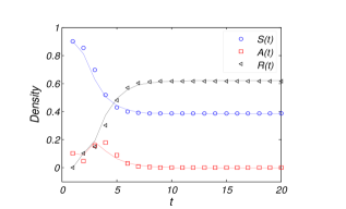
Figure 1: Time evolutions of densities of nodes in different states, denoted by $S(t)$ (blue circles), $A(t)$ (red squares), and $R(t)$ (black left triangles), respectively. Analytical results are plotted in lines, which match well with simulation results (symbols). The parameters for the simulations are $N$=10,000, $\langle k\rangle$ = 10, $\langle w\rangle$ = 8, $\alpha_{k}$=2.1, $\alpha_{w}$=2.4, $\beta$=0.18, $A_{0}$=0.1 and $T$=3.

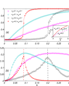
Figure 2: Final states of complex contagion dynamics on weighted networks. (a) Final adoption size ($R(\infty)$) versus the unit transmission probability ($\beta$) on different networks with tunable parameters. The inset shows the numerical solutions of mean transmission rate $\langle\lambda_{w}\rangle$ as function of $\beta$ for three different values of $\alpha_{w}$ (i.e., 2.1, 2.5, and 4.0). (b) Final subcritical size ($A_{T-1}(\infty)$) versus the $\beta$ on different networks with tunable parameters. The parameters for all the simulations are $N$=10,000, $\langle k\rangle$ = 10, $\langle w\rangle$ = 8, $A_{0}$=0.1 and $T$=3.

Figure 1 illustrates the time evolutions of susceptible (S), adopted (A) and recovered (R) nodes. Naturally, it displays a very similar dynamics with SIR model. Our analytical results (lines) agree well with simulation results (symbols). In Fig. 2(a), we show the final adoption size ($R(\infty)$) in relationship with unit transmission probability ($\beta$) for networks with different degree and weight distributions along with the analytical results (shown in black line, which match well with the simulation results). Now, let us focus on the influence of heterogeneous degree distribution on social contagion processes from two perspectives: the transition type of $R(\infty)$ with $\beta$ and the final adoption size. We summarise our results as following.

First, the degree exponent determine the discontinuity of the transition as shown in a previous work Wang et al. (2015c). Figure 2(a) shows that $R(\infty)$ increases continuously with $\beta$ with heterogeneous degree distribution (e.g., $\alpha_{k}=2.1$), while exhibiting a discontinuous transition when $\alpha_{k}=4.0$. The results of bifurcation analysis on Eq. (15) show that there exists one critical degree exponent $\alpha_{k}^{c}\approx 4.0$, below (above) which $R(\infty)$ versus $\beta$ is continuous (discontinuous). For networks with $\alpha_{k}=4.0$, the value of $\beta_{c}$ can be obtained from Eq. (15) using bifurcation theory Strogatz (2014). Analytical calculations show that for Eq. (15), the number of roots in Eq. (15) is either one or three (see Fig. 3). If Eq. (15) has only one root, $R(\infty)$ increases continuously with $\beta$; if Eq. (15) has three roots, a saddle-node bifurcation occursStrogatz (2014). As shown in Fig. 3, there is only one fixed point of Eq. (15) at a small value of $\beta$ (e.g, $\beta=0.1984$) and then three fixed points (in this case, only the maximum one is physically meaningful since $\theta(t)$ decreases with $t$) gradually emerge with the increasing of $\beta$. The tangent point that marked as one red circle is the physically meaningful solution at the unit transmission probability $\beta_{c}$ (e.g, $\beta=0.2006$). For $\beta>\beta_{c}$ (e.g, $\beta=0.2039$), the solution of Eq. (15) changes to a smaller solution abruptly, which leads to a discontinuous change in $R(\infty)$. We can demonstrate the type of dependence and obtain the value of $\beta_{c}$ for other parameters through the similar measure.

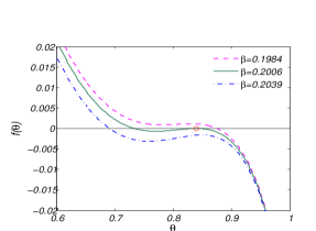
Figure 3: Illustration of graphical solutions of Eq. (15). The black solid line is the horizontal axis and the red circle denotes the tangent point. The parameters for the simulations are $N$=10,000, $\langle k\rangle$ = 10, $\langle w\rangle$ = 8, $\alpha_{k}=4.0$, $\alpha_{w}=2.1$, $A_{0}$=0.1 and $T$=3.

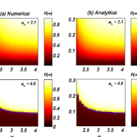
Figure 4: The relationships between $\alpha_{w}$, $\beta$ and $R(\infty)$ at a fixed $\alpha_{k}$. Figures (a) and (b) are results of numerical simulation and analytical method on networks with two different $\alpha_{k}$ (i.e., 2.1 and 4.0) respectively. The parameters for simulation are $N$=10,000, $\langle k\rangle$ = 10, $\langle w\rangle$ = 8, $A_{0}$=0.1 and $T$=3.

We also explain this phenomena visually by showing $A_{T-1}(\infty)$ (final subcritical size) in Fig. 2(b). Here nodes with awareness value $T-1$ are considered as in subcritical state. Clearly, for results of $\alpha_{k}=4.0$ in Fig. 2(b), the quick sharp decline of final subcritical size corresponds to a dramatic increase of final adoption size, thus may induce a discontinuous dependence. Note that, there is no so-called critical value of unit transmission probability ($\beta_{c}$) for continuous dependence. The critical value $\beta_{c}$ can also be estimated by increasing the number of iterations Parshani et al. (2011) (only those interactions in which appears at least one newly adopted individual are taken into account). In Fig. 2(b), we show the estimated $\beta_{c}$ with dashed lines, which correspond to the peaks of $A_{T-1}(\infty)$. More details are shown in Fig. 4. As we expected, $R(\infty)$ for networks with heterogeneous degree distribution (Fig. 4(a) above) shows a continuous change with the increasing of $\beta$ while change discontinuously on networks with homogeneous degree distribution (Fig. 4(a) below). Analytical results shown in Fig. 4(b) agree well with numerical results. The estimated values of $\beta_{c}$ are labeled in blue circle, along with the corresponding analytical critical results are plotted in blue line (shown in Figs. 4(b)).

Second, as a result of continuous-discontinuous transition, degree heterogeneity enhances the final adoption size at small $\beta$ while hindering it at large $\beta$, which is consistent with that of epidemic case Wang et al. (2014). For instance, when $\alpha_{w}=2.1$, the final adoption size ($R(\infty)$) for $\alpha_{k}=2.1$ is greater than that of $\alpha_{k}=4.0$ when $\beta<0.2$, while opposite situation is obtained when $\beta>0.2$ (shown in Fig. 2(a)). This result can be qualitatively explained as following: social contagion propagates on complex networks in two-stages due to the co-emergence of more hubs and large amount of small-degree nodes with increasing heterogeneity of degree distribution. The hubs are more likely to become adopted early since more neighbors make them have higher chance to reach the identical awareness threshold $T$ thus get adopted. On the contrary, small-degree nodes are less likely to become adopted due to the small number of its neighbors. Given a network with heterogeneous degree distribution, when unit transmission probability $\beta$ is small, the existence of more hubs enhance the contagion thus leads to greater $R(\infty)$ (promotion region); When $\beta$ is large, the existence of large amount of small-degree nodes will hinder the contagion, resulting in smaller $R(\infty)$ (suppression region). Fig. 5 shows the whole picture of relationship between $\alpha_{k}$, $\beta$ and $R(\infty)$ when fixing $\alpha_{w}$. Increasing the heterogeneity of degree distribution will enhance $R(\infty)$ at small $\beta$ while hinder the adoption size at large $\beta$.

Figure 5: The relationships between $\alpha_{k}$, $\beta$ and $R(\infty)$ at a fixed $\alpha_{w}$. Figures (a) and (b) are results of numerical simulation and analytical method on networks with two different $\alpha_{w}$ (i.e., 2.1 and 4.0), respectively. The parameters for the simulations are $N$=10,000, $\langle k\rangle$ = 10, $\langle w\rangle$ = 8, $A_{0}$=0.1 and $T$=3.

Let us address the influence of the heterogeneity of weight distribution on social contagion processes at a given $\alpha_{k}$. The heterogeneity of weight distribution (smaller value of $\alpha_{w}$) reduces final adoption size $R(\infty)$. For instance, if we fix $\alpha_{k}$ (Fig. 2(a)), $R(\infty)$ for $\alpha_{w}=2.1$ is always smaller than that of $\alpha_{w}=4.0$. This phenomenon can be explained as follows: when the average weight $\langle w\rangle$ is fixed, in the network with smaller $\alpha_{w}$, most edges have lower weights and thus transmission probabilities, leading to a smaller mean transmission rate $\langle\lambda_{w}\rangle=\sum_{w}g(w)\lambda_{w}$ for a randomly selected edge. As shown in the inset of Fig. 2(a), $\langle\lambda_{w}\rangle$ of $\alpha_{w}$=2.1 is smaller than that of $\alpha_{w}=4.0$ with a given $\beta$. On the other hand, changing the weight distribution will not change the dependence behavior of ($R(\infty)$, $\beta$) with a given degree distribution, which is similar to the case of simple contagion models Wang et al. (2014). This finding can be verified from analytical perspective, varying the value of $\alpha_{w}$ will not change the number of roots in Eq. (15), thus will not affect whether saddle-node bifurcation occur or not. The relationship between $\alpha_{w}$ and $\beta$ when fixing $\alpha_{k}$ is shown in Fig 4, which confirms our finding here.

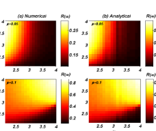
Figure 6: The relationships between $\alpha_{k}$, $\alpha_{w}$ and $R(\infty)$ when the unit transmission probability $\beta$ is fixed. Figures (a) and (b) are results of numerical simulation and analytical method on the weighted contagion model with two different $\beta$ (i.e., 0.05 and 0.1), respectively. The parameters for the simulations are $N$=10,000, $\langle k\rangle$ = 10, $\langle w\rangle$ = 8, $A_{0}$=0.1 and $T$=3.

Finally, Fig. 6 summarizes our results, showing that for small value of transmission probability ($\beta=0.05$), the existence of more hubs that can be easily informed thus enhance the contagion process (Promotion Region). While for large value of transmission probability ($\beta=0.1$), the existence of large-amount small-degree nodes that difficult to be adopted will hinder the contagion process (Suppression Region). In addition, increasing the heterogeneity of weight distribution will always hinder $R(\infty)$. Figs. 6(a) and 6(b) show results of simulation and analytical method respectively, which match well with each other.

IV Conclusions

In summary, we study the effect of heterogenous network structures on the diffusion of complex contagions. With decreasing heterogeneity of degree distribution, the dependence of final adoption size on unit transmission probability changes from being continuous to discontinuous. We then show that the heterogeneity of degree distribution may have two opposite effects depending on the transmission probability: degree heterogeneity enhances complex contagions when $\beta$ is small while hindering it when $\beta$ is large. By contrast, the heterogeneity of weight distribution always reduces final adoption size though not change the dependence pattern of final adoption size on unit transmission probability.

Our findings offer insights to understand the influence of underlying network structures for weighed social contagions. Future work may investigate into the cases where the adoption threshold of each individual varies with its degree, or a richer and correlated network structure is assumed.