Embedding Lexical Features via Low-Rank Tensors

Abstract

Modern NLP models rely heavily on engineered features, which often combine word and contextual information into complex lexical features. Such combination results in large numbers of features, which can lead to over-fitting. We present a new model that represents complex lexical features—comprised of parts for words, contextual information and labels—in a tensor that captures conjunction information among these parts. We apply low-rank tensor approximations to the corresponding parameter tensors to reduce the parameter space and improve prediction speed. Furthermore, we investigate two methods for handling features that include $n$-grams of mixed lengths. Our model achieves state-of-the-art results on tasks in relation extraction, PP-attachment, and preposition disambiguation.

1 Introduction

Statistical NLP models usually rely on hand-designed features, customized for each task. These features typically combine lexical and contextual information with the label to be scored. In relation extraction, for example, there is a parameter for the presence of a specific relation occurring with a feature conjoining a word type (lexical) with dependency path information (contextual). In measuring phrase semantic similarity, a word type is conjoined with its position in the phrase to signal its role. Figure 1b shows an example in dependency parsing, where multiple types (words) are conjoined with POS tags or distance information.

To avoid model over-fitting that often results from features with lexical components, several smoothed lexical representations have been proposed and shown to improve performance on various NLP tasks; for instance, word embeddings [Bengio et al. (2006] help improve NER, dependency parsing and semantic role labeling [Miller et al. (2004, Koo et al. (2008, Turian et al. (2010, Sun et al. (2011, Roth and Woodsend (2014, Hermann et al. (2014].

However, using only word embeddings is not sufficient to represent complex lexical features (e.g. $\phi$ in Figure 1c). In these features, the same word embedding conjoined with different non-lexical properties may result in features indicating different labels; the corresponding lexical feature representations should take the above interactions into consideration. Such important interactions also increase the risk of over-fitting as feature space grows exponentially, yet how to capture these interactions in representation learning remains an open question.

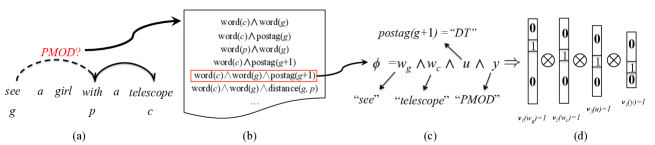
Figure 1: An example of lexical features used in dependency parsing. To predict the “PMOD” arc (the dashed one) between “see” and “with” in (a), we may rely on lexical features in (b). Here $p$, $c$, $g$ are indices of the word “with”, its child (“telescope”) and a candidate head. Figure (c) shows what the fifth feature ($\phi$) is like, when the candidate is “see”. As is common in multi-class classification tasks, each template generates a different feature for each label y. Thus a feature $\phi=\textrm{w}_{g}\wedge\textrm{w}_{c}\wedge\textrm{u}\wedge\textrm{y}$ is the conjunction of the four parts. Figure (d) is the one-hot representation of $\phi$, which is equivalent to the outer product (i.e. a 4-way tensor) among the four one-hot vectors. $\mathbf{v}(x)=1$ means the vector $\mathbf{v}$ has a single non-zero element in the $x$ position.

To address the above problems, we propose a general and unified approach to reduce the feature space by constructing low-dimensional feature representations, which provides a new way of combining word embeddings, traditional non-lexical properties, and label information. Our model exploits the inner structure of features by breaking the feature into multiple parts: lexical, non-lexical and (optional) label. We demonstrate that the full feature is an outer product among these parts. Thus, a parameter tensor scores each feature to produce a prediction. Our model then reduces the number of parameters by approximating the parameter tensor with a low-rank tensor: the Tucker approximation of ?) but applied to each embedding type (view), or the Canonical/Parallel-Factors Decomposition (CP). Our models use fewer parameters than previous work that learns a separate representation for each feature [Ando and Zhang (2005, Yang and Eisenstein (2015]. CP approximation also allows for much faster prediction, going from a method that is cubic in rank and exponential in the number of lexical parts, to a method linear in both. Furthermore, we consider two methods for handling features that rely on $n$-grams of mixed lengths.

Our model makes the following contributions when contrasted with prior work:

?) applied CP to combine different views of features. Compared to their work, our usage of CP-decomposition is different in the application to feature learning: (1) We focus on dimensionality reduction of existing, well-verified features, while ?) generates new features (usually different from ours) by combining some “atom” features. Thus their work may ignore some useful features; it relies on binary features as supplementary but our model needs not. (2) ?)’s factorization relies on views with explicit meanings, e.g. head/modifier/arc in dependency parsing, making it less general. Therefore its applications to tasks like relation extraction are less obvious.

Compared to our previous work [Gormley et al. (2015, Yu et al. (2015], this work allows for higher-order interactions, mixed-length n-gram features, lower-rank representations. We also demonstrate the strength of our new model via applications to new tasks.

The resulting method learns smoothed feature representations combining lexical, non-lexical and label information, achieving state-of-the-art performance on several tasks: relation extraction, preposition semantics and PP-attachment.

2 Notation and Definitions

We begin with some background on notation and definitions. Let $\mathcal{T}\in\mathbb{R}^{d_{1}\times\cdots\times d_{K}}$ be a $K$-way tensor (i.e., a tensor with $K$ views). In this paper, we consider the tensor $k$-mode product, i.e. multiplying a tensor $\mathcal{T}\in\mathbb{R}^{d_{1}\times\cdots\times d_{K}}$ by a matrix $\mathbf{x}\in\mathbb{R}^{d_{k}\times J}$ (or a vector if $J=1$) in mode (view) $k$. The product is denoted by $\mathcal{T}\times_{k}\mathbf{x}$ and is of size $d_{1}\times\cdots\times d_{k-1}\times J\times d_{k+1}\times\cdots\times d_{K}$. Element-wise, we have

$$(\mathcal{T}\times_{k}\mathbf{x})_{i_{1}\ldots i_{k-1}\ j\ i_{k+1}\ldots i_{K}}=\sum_{i_{k}=1}^{d_{k}}\mathcal{T}_{i_{1}\ldots i_{k}\ldots i_{K}}\mathbf{x}_{i_{k}j},$$

for $j=1,\ldots,J$. A mode-$k$ fiber $\mathcal{T}_{i_{1}\ldots i_{k-1}\bullet i_{k+1}\ldots i_{K}}$ of $\mathcal{T}$ is the $d_{k}$ dimensional vector obtained by fixing all but the $k$th index. The mode-$k$ unfolding $\mathcal{T}_{(k)}$ of $\mathcal{T}$ is the $d_{k}\times\prod_{i\neq k}d_{i}$ matrix obtained by concatenating all the $\prod_{i\neq k}d_{i}$ mode-$k$ fibers along columns.

Given two matrices $\textrm{W}_{\mkern-4.0mu1}\in\mathbb{R}^{d_{1}\times r_{1}},\textrm{W}_{\mkern-4.0mu2}\in\mathbb{R}^{d_{2}\times r_{2}}$, we write $\textrm{W}_{\mkern-4.0mu1}\otimes\textrm{W}_{\mkern-4.0mu2}$ to denote the Kronecker product between $\textrm{W}_{\mkern-4.0mu1}$ and $\textrm{W}_{\mkern-4.0mu2}$ (outer product for vectors). We define the Frobenius product (matrix dot product) $\mathbf{A}\odot\mathbf{B}=\sum_{i,j}A_{ij}B_{ij}$ between two matrices with the same sizes; and define element-wise (Hadamard) multiplication $\mathbf{a}\circ\mathbf{b}$ between vectors with the same sizes.

Tucker Decomposition:

Tucker Decomposition represents a $d_{1}\times d_{2}\times\ldots\times d_{K}$ tensor $\mathcal{T}$ as:

$${\mathcal{T}} =g\times_{1}\textrm{W}_{\mkern-4.0mu1}\times_{2}\textrm{W}_{\mkern-4.0mu2}\ldots\times_{K}\textrm{W}_{\mkern-4.0muK}$$ (1)

where each $\times_{i}$ is the tensor $i$-mode product and each $\textrm{W}_{\mkern-4.0mui}$ is a $r_{i}\times d_{i}$ matrix. Tensor $g$ with size $r_{1}\times r_{2}\times\ldots\times r_{K}$ is called the core tensor. We say that ${\mathcal{T}}$ has a Tucker rank $(r_{(1)},r_{(2)},\ldots,r_{(K)})$, where $r_{(i)}=\textrm{rank}({{\mathcal{T}}}_{(i)})$ is the rank of mode-$i$ unfolding. To simplify learning, we define the Tucker rank as $r_{(i)}$$=$rank($\mathbf{g}_{(i)}$), which can be bounded simply by the dimensions of $g$, i.e. $r_{(i)}\leq r_{i}$; this allows us to enforce a rank constraint on $\mathcal{T}$ simply by restricting the dimensions $r_{i}$ of $g$, as described in §6.

CP Decomposition:

CP decomposition represents a $d_{1}$$\times$$d_{2}$$\times$$\ldots$$\times$$d_{K}$ tensor $\mathcal{T}$ as a sum of rank-one tensors (i.e. a sum of outer products of $K$ vectors):

$${\mathcal{T}}=\sum_{j=1}^{r}\textrm{W}_{\mkern-4.0mu1}[j,:]\otimes\textrm{W}_{\mkern-4.0mu2}[j,:]\otimes\ldots\otimes\textrm{W}_{\mkern-4.0muK}[j,:]$$ (2)

where each $\textrm{W}_{\mkern-4.0mui}$ is an $r\times d_{i}$ matrix and $\textrm{W}_{\mkern-4.0mui}[j,:]$ is the vector of its $j$-th row. For CP decomposition, the rank $r$ of a tensor ${\mathcal{T}}$ is defined to be the number of rank-one tensors in the decomposition. CP decomposition can be viewed as a special case of Tucker decomposition in which $r_{1}=r_{2}=\ldots=r_{K}=r$ and $g$ is a superdiagonal tensor.

3 Factorization of Lexical Features

Suppose we have feature $\phi$ that includes information from a label y, multiple lexical items $\textrm{w}_{1},\ldots,\textrm{w}_{n}$ and non-lexical property u. This feature can be factorized as a conjunction of each part: $\phi=\textrm{y}\wedge\textrm{u}\wedge\textrm{w}_{1}\wedge\ldots\wedge\textrm{w}_{n}$. The feature fires when all $(n+2)$ parts fire in the instance (reflected by the $\wedge$ symbol in $\phi$). The one-hot representation of $\phi$ can then be viewed as a tensor $e_{\phi}=\textrm{y}\otimes\textrm{u}\otimes\textrm{w}_{1}\otimes\cdots\otimes\textrm{w}_{n}$, where each feature part is also represented as a one-hot vector. Figure 1d illustrates this case with two lexical parts.

Given an input instance $\mathbf{x}$ and its associated label y, we can extract a set of features $S(\mathbf{x},\textrm{y})$. In a traditional log-linear model, we view the instance $\mathbf{x}$ as a bag-of-features, i.e. a feature vector $F(\mathbf{x},\textrm{y})$. Each dimension corresponds to a feature $\phi$, and has value 1 if $\phi\in S(\mathbf{x},\textrm{y})$. Then the log-linear model scores the instance as $s(\mathbf{x},\textrm{y};\mathbf{w})=\mathbf{w}^{T}F(\mathbf{x},\textrm{y})=\sum_{\phi\in S(\mathbf{x},\textrm{y})}s(\phi;\mathbf{w})$, where $\mathbf{w}$ is the parameter vector. We can re-write $s(\mathbf{x},\textrm{y};\mathbf{w})$ based on the factorization of the features using tensor multiplication; in which $\mathbf{w}$ becomes a parameter tensor $\mathcal{T}$:

$$s(\mathbf{x},\textrm{y};\mathbf{w})=s(\mathbf{x},\textrm{y};\mathcal{T})=\sum_{\phi\in S(\mathbf{x},\textrm{y})}s(\phi;\mathcal{T})$$ (3)

Here each $\phi$ has the form $(\textrm{y},\textrm{u},\textrm{w}_{1},\ldots,\textrm{w}_{n})$, and

$$s(\phi;\mathcal{T})=\mathcal{T}\times_{l}\textrm{y}\times_{f}\textrm{u}\times_{\textrm{w}_{1}}\textrm{w}_{1}...\times_{\textrm{w}_{n}}\textrm{w}_{n}.$$ (4)

Note that one-hot vectors $\textrm{w}_{i}$ of words themselves are large ($|\textrm{w}_{i}|>$ 500k), thus the above formulation with parameter tensor $\mathcal{T}$ can be very large, making parameter estimation difficult. Instead of estimating only the values of the dimensions which appear in training data as in traditional methods, we will reduce the size of tensor $\mathcal{T}$ via a low-rank approximation. With different approximation methods, (4) will have different equivalent forms, e.g. (6), (7) in §4.1.

Optimization objective:

The loss function $\ell$ for training the log-linear model uses (3) for scores, e.g., the log-loss $\ell(\mathbf{x},\textrm{y};\mathcal{T})=-\log\frac{\exp\{s(\mathbf{x},\textrm{y};\mathcal{T})\}}{\sum_{\textrm{y}^{\prime}\in L}\exp\{s(\mathbf{x},\textrm{y}^{\prime};\mathcal{T})\}}$. Learning can be formulated as the following optimization problem:

$$\begin{aligned} &\underset{\mathcal{T}}{\textrm{minimize:}}&&\sum_{(\mathbf{x},y)\in\mathcal{D}}\ell(\mathbf{x},y;\mathcal{T})\\ &\textrm{subject to:}&&\left\{\begin{matrix}\textrm{rank}({\mathcal{T}})\leq(r_{1},r_{2},...,r_{n+2})\\ \text{\quad\quad\quad\quad\quad(Tucker-form)}\\ \textrm{rank}({\mathcal{T}})\leq r\text{\quad(CP-form)}\end{matrix}\right.\end{aligned}$$ (5)

where the constraints on rank($\mathcal{T}$) depend on the chosen tensor approximation method (§2).

The above framework has some advantages: First, as discussed in §1 and here, we hope the representations capture rich interactions between different parts of the lexical features; the low-rank tensor approximation methods keep the most important interaction information of the original tensor, while significantly reducing its size. Second, the low-rank structure will encourage weight-sharing among lexical features with similar decomposed parts, leading to better model generalization. Note that there are examples where features have different numbers of multiple lexical parts, such as both unigram and bigram features in PP-attachment. We will use two different methods to handle these features (§5).

Remarks (advantages of our factorization)

Compared to prior work, e.g. [Lei et al. (2014, Lei et al. (2015], the proposed factorization has the following advantages:

1. Parameter explosion when mapping a view with lexical properties to its representation vector (as will be discussed in 4.3): Our factorization allows the model to treat word embeddings as inputs to the views of lexical parts, dramatically reducing the parameters. Prior work cannot do this since its views are mixtures of lexical and non-lexical properties. Note that ?) uses embeddings by concatenating them to specific views, which increases dimensionality, but the improvement is limited.

2. No weight-sharing among conjunctions with same lexical property, like the child-word “word($c$)” and its conjunction with head-postag “word($c$) $\wedge$ word($g$)” in Figure 1(b). The factorization in prior work treats them as independent features, greatly increasing the dimensionality. Our factorization builds representations of both features based on the embedding of “word($c$)”, thus utilizing their connections and reducing the dimensionality.

The above advantages are also key to overcome the problems of prior work mentioned at the end of §1.

4 Feature Representations via Low-rank Tensor Approximations

Using one-hot encodings for each of the parts of feature $\phi$ results in a very large tensor. This section shows how to compute the score in (4) without constructing the full feature tensor using two tensor approximation methods (§4.1 and §4.2).

We begin with some intuition. To score the original (full rank) tensor representation of $\phi$, we need a parameter tensor $\mathcal{T}$ of size $d_{1}\times d_{2}\times\ldots\times d_{n+2}$, where $d_{3}=\cdots=d_{n+2}=|V|$ is the vocabulary size, $n$ is the number of lexical parts in the feature and $d_{1}=|L|$ and $d_{2}=|F|$ are the number of different labels and non-lexical properties, respectively. (§5 will handle $n$ varying across features.) Our methods reduce the tensor size by embedding each part of $\phi$ into a lower dimensional space, where we represent each label, non-lexical property and words with an $r_{1},r_{2}$, $r_{3},\ldots,r_{n+2}$ dimensional vector respectively ($r_{i}\ll d_{i}$, $\forall i$). These embedded features can then be scored by much smaller tensors. We denote the above transformations as matrices $\textrm{W}_{\mkern-4.0mu\l}\in\mathbb{R}^{r_{1}\times d_{1}}$, $\textrm{W}_{\mkern-4.0muf}\in\mathbb{R}^{r_{2}\times d_{2}}$, $\textrm{W}_{\mkern-4.0mui}\in\mathbb{R}^{r_{i+2}\times d_{i+2}}$ for $i=1,\ldots,n$, and write corresponding low-dimensional hidden representations as $\mathbf{h}^{(\l)}_{\textrm{y}}=\textrm{W}_{\mkern-4.0mu\l}\textrm{y}$, $\mathbf{h}^{(f)}_{\textrm{u}}=\textrm{W}_{\mkern-4.0muf}\textrm{u}$ and $\mathbf{h}^{(i)}_{\textrm{w}}=\textrm{W}_{\mkern-4.0mui}\textrm{w}$.

In our methods, the above transformations of embeddings are parts of low-rank tensors as in (5), so the embeddings of non-lexical properties and labels can be trained simultaneously with the low-rank tensors. Note that for one-hot input encodings the transformation matrices are essentially lookup tables, making the computation of these transformations sufficiently fast.

4.1 Tucker Form

For our first approximation, we assume that tensor $\mathcal{T}$ has a low-rank Tucker decomposition: $\mathcal{T}=g\times_{\l}\textrm{W}_{\mkern-4.0mu\l}\times_{f}\textrm{W}_{\mkern-4.0muf}\times_{\textrm{w}_{1}}\textrm{W}_{\mkern-4.0mu1}\times_{\textrm{w}_{2}}\cdots\times_{\textrm{w}_{n}}\textrm{W}_{\mkern-4.0mun}$. We can then express the scoring function (4) for a feature $\phi=(\textrm{y},\textrm{u},\textrm{w}_{1},\ldots\textrm{w}_{n})$ with $n$-lexical parts, as:

$$\textstyle\!s(\textrm{y},\textrm{u},\textrm{w}_{1},\cdots,\textrm{w}_{n};g,{\textrm{W}_{\mkern-4.0mu\l}},{\textrm{W}_{\mkern-4.0muf}},{\{\textrm{W}_{\mkern-4.0mui}\}_{i=1}^{n}})$$

$$= \ g\times_{\l}\mathbf{h}^{(\l)}_{\textrm{y}}\times_{f}\mathbf{h}^{(f)}_{\textrm{u}}\times_{\textrm{w}_{1}}\mathbf{h}^{(1)}_{\textrm{w}_{1}}\cdots\times_{\textrm{w}_{n}}\mathbf{h}^{(n)}_{\textrm{w}_{n}},$$ (6)

which amounts to first projecting $\textrm{u},\textrm{y}$, and $\textrm{w}_{i}$ (for all $i$) to lower dimensional vectors $\mathbf{h}^{(f)}_{\textrm{u}},\mathbf{h}^{(\l)}_{\textrm{y}},\mathbf{h}^{(i)}_{\textrm{w}_{i}}$, and then weighting these hidden representations using the flattened core tensor $g$. The low-dimensional representations and the corresponding weights are learned jointly using a discriminative (supervised) criterion. We call the model based on this representation the Low-Rank Feature Representation with Tucker form, or lrfr_n-tucker.

4.2 CP Form

For the Tucker approximation the number of parameters in (6) scale exponentially with the number of lexical parts. For instance, suppose each $\mathbf{h}^{(i)}_{\textrm{w}_{i}}$ has dimensionality $r$, then $|g|\propto r^{n}$. To address scalability and further control the complexity of our tensor based model, we approximate the parameter tensor using CP decomposition as in (2), resulting in the following scoring function:

$$s(\textrm{y},\textrm{u},\textrm{w}_{1},\cdots,\textrm{w}_{n};{\textrm{W}_{\mkern-4.0mu\l}},{\textrm{W}_{\mkern-4.0muf}},{\{\textrm{W}_{\mkern-4.0mui}\}_{i=1}^{n}})=$$

$$\qquad\sum_{j=1}^{r}\left(\mathbf{h}^{(\l)}_{\textrm{y}}\circ\mathbf{\mathbf{h}^{(f)}_{\textrm{u}}}\circ\mathbf{h}^{(1)}_{\textrm{w}_{1}}\circ\cdots\circ\mathbf{h}^{(n)}_{\textrm{w}_{n}}\right)_{j}.$$ (7)

We call this model Low-Rank Feature Representation with CP form (lrfr_n-cp).

4.3 Pre-trained Word Embeddings

One of the computational and statistical bottlenecks in learning these lrfr_n models is the vocabulary size; the number of parameters to learn in each matrix $\textrm{W}_{\mkern-4.0mui}$ scales linearly with $|V|$ and would require very large sets of labeled training data. To alleviate this problem, we use pre-trained continuous word embeddings [Mikolov et al. (2013] as input embeddings rather than the one-hot word encodings. We denote the $m$-dimensional word embeddings by $e_{\textrm{w}}$; so the transformation matrices $\textrm{W}_{\mkern-4.0mui}$ for the lexical parts are of size $r_{i}\times m$ where $m\ll|V|.$

We note that when sufficiently large labeled data is available, our model allows for fine-tuning the pre-trained word embeddings to improve the expressive strength of the model, as is common with deep network models.

Remarks

Our lrfrs introduce embeddings for non-lexical properties and labels, making them better suit the common setting in NLP: rich linguistic properties; and large label sets such as open-domain tasks [Hoffmann et al. (2010]. The lrfr-cp better suits $n$-gram features, since when $n$ increases 1, the only new parameters are the corresponding $\textrm{W}_{\mkern-4.0mui}$. It is also very efficient during prediction ($O(nr)$), since the cost of transformations can be ignored with the help of look-up tables and pre-computing.

5 Learning Representations for $n$-gram Lexical Features of Mixed Lengths

For features with $n$ lexical parts, we can train an lrfr_n model to obtain their representations. However, we often have features of varying $n$ (e.g. both unigrams ($n$=1) and bigrams ($n$=2) as in Figure 1). We require representations for features with arbitrary different $n$ simultaneously.

We propose two solutions. The first is a straightforward solution based on our framework, which handles each $n$ with a $(n+2)$-way tensor. This strategy is commonly used in NLP, e.g. ?) have different kernel functions for different order of dependency features. The second is an approximation method which aims to use a single tensor to handle all $n$s.

Multiple Low-Rank Tensors

Suppose that we can divide the feature set $S(\mathbf{x},\textrm{y})$ into subsets $S_{1}(\mathbf{x},\textrm{y}),S_{2}(\mathbf{x},\textrm{y}),\ldots,S_{n}(\mathbf{x},\textrm{y})$ which correspond to features with one lexical part (unigram features), two lexical parts (bigram features)$,\ldots$ and $n$ lexical parts ($n$-gram features), respectively. To handle these types of features, we modify the training objective as follows:

$$\underset{\mathcal{T}_{1},\mathcal{T}_{2},\cdots,\mathcal{T}_{n}}{\textrm{minimize}}{\sum_{(\mathbf{x},\textrm{y})\in D}\ell(\mathbf{x},\textrm{y};\mathcal{T}_{1},\mathcal{T}_{2},\ldots,...\mathcal{T}_{n})},$$ (8)

where the score of a training instance $(\mathbf{x},\textrm{y})$ is defined as $s(\mathbf{x},\textrm{y};\mathcal{T})=\sum_{i=1}^{n}\sum_{\phi\in S_{i}(\mathbf{x},\textrm{y})}s(\phi;\mathcal{T}_{i})$. We use the Tucker form low-rank tensor for $\mathcal{T}_{1}$, and the CP form for $\mathcal{T}_{i}$ $(\forall i>1)$. We refer to this method as lrfr₁-tucker & lrfr₂-cp.

Word Clusters

Alternatively, to handle different numbers of lexical parts, we replace some lexical parts with discrete word clusters. Let $c(\textrm{w})$ denote the word cluster (e.g. from Brown clustering) for word w. For bigram features we have:

$$\hskip 1.0pt\textstyle s(\textrm{y},\textrm{u},{\textrm{w}}_{1},\textrm{w}_{2};{\mathcal{T}})$$

$$\textstyle=s(\textrm{y},\textrm{u}\!\wedge\!c(\textrm{w}_{1}),\textrm{w}_{2};{\mathcal{T}})+s(\textrm{y},\textrm{u}\!\wedge\!c(\textrm{w}_{2}),\textrm{w}_{1};{\mathcal{T}})$$

$$\textstyle={\mathcal{T}}\times_{\l}\textrm{y}\times_{f}\left(\textrm{u}\wedge c(\textrm{w}_{1})\right)\times_{\textrm{w}}e_{\textrm{w}_{2}}$$

$$\textstyle\qquad+{\mathcal{T}}\times_{\l}\textrm{y}\times_{f}\left(\textrm{u}\wedge c(\textrm{w}_{2})\right)\times_{\textrm{w}}e_{\textrm{w}_{1}}$$ (9)

where for each word we have introduced an additional set of non-lexical properties that are conjunctions of word clusters and the original non-lexical properties. This allows us to reduce an $n$-gram feature representation to a unigram representation. The advantage of this method is that it uses a single low-rank tensor to score features with different numbers of lexical parts. This is particularly helpful when we have very limited labeled data. We denote this method as lrfr₁-Brown, since we use Brown clusters in practice. In the experiments we use the Tucker form for lrfr₁-Brown.

6 Parameter Estimation

The goal of learning is to find a tensor $\mathcal{T}$ that solves problem (5). Note that this is a non-convex objective, so compared to the convex objective in a traditional log-linear model, we are trading better feature representations with the cost of a harder optimization problem. While stochastic gradient descent (SGD) is a natural choice for learning representations in large data settings, problem (5) involves rank constraints, which require an expensive proximal operation to enforce the constraints at each iteration of SGD. We seek a more efficient learning algorithm. Note that we fixed the size of each transformation matrix $\textrm{W}_{\mkern-4.0mui}\in\mathbb{R}^{r_{i}\times d_{i}}$ so that the smaller dimension ($r_{i}$ $<$ $d_{i}$) matches the upper bound on the rank. Therefore, the rank constants are always satisfied through a run of SGD and we in essence have an unconstrained optimization problem. Note that in this way we do not guarantee orthogonality and full-rank of the learned transformation matrices. These properties are assumed in general, but are not necessary according to [Kolda and Bader (2009].

The gradients are computed via the chain-rule. We use AdaGrad [Duchi et al. (2011] and apply L2 regularization on all $\textrm{W}_{\mkern-4.0mui}$s and $g$, except for the case of $r_{i}$=$d_{i}$, where we will start with $\textrm{W}_{\mkern-4.0mui}=\mathbf{I}$ and regularize with $\|\textrm{W}_{\mkern-4.0mui}$ - $\mathbf{I}\|_{2}$. We use early-stopping on a development set.

7 Experimental Settings

Task	Benchmark	Dataset	Numbers on Each View
			#Labels ($d_{1}$)	#Non-lexical Features ($d_{2}$)
Relation Extraction	?)	ACE 2005	32	264
PP-attachment	?)	WSJ	-	1,213 / 607
Preposition Disambiguation	?)	?)	6	9/3

Table 1: Statistics of each task. PP-attachment and preposition disambiguation have both unigram and bigram features. Therefore we list the numbers of non-lexical properties for both types.

Set	Template
HeadEmb	$\{I[i=h_{1}],I[i=h_{2}]\}$ (head of $M_{1}/M_{2}$)
	$\&\{\phi,t_{h_{1}},t_{h_{2}},t_{h_{1}}\&t_{h_{2}}\}$
Context	$I[i=h_{1}/h_{2}\pm 1]$ (left/right token of $w_{h_{1}/h_{2}}$)
In-between	$I[i>h_{1}]\&I[i<h_{2}]$$\&\{\phi,t_{h_{1}},t_{h_{2}},t_{h_{1}}\&t_{h_{2}}\}$
On-path	$I[w_{i}\in P]$ $\&\{\phi,t_{h_{1}},t_{h_{2}},t_{h_{1}}\&t_{h_{2}}\}$
Set	Template
Bag of Words	$w$, $p$ $\&$ $w$ ($w$ is $w_{m}$ or $w_{h}$)
Word-Position	$w_{m}$, $w_{h}$, $w_{m}$ $\&$ $w_{h}$
Preposition	$p$, $p$ $\&$ $w_{m}$, $p$ $\&$ $w_{h}$, $p$ $\&$ $w_{m}$ $\&$ $w_{h}$

Set	Template
Bag of Words	$w$ ($w$ is $w_{m}$ or $w_{h}$), $w_{m}\&w_{h}$
Distance	Dis$(w_{h},w_{m})$ $\&$ $\{w_{m},w_{h},w_{m}\&w_{h}\}$
Prep	$w_{p}$ $\&$ $\{w_{m},w_{h},w_{m}\&w_{h}\}$
POS	$t(w_{h})$ $\&$ $\{w_{m},w_{h},w_{m}\&w_{h}\}$
NextPOS	$t(w_{h+1})$ $\&$ $\{w_{m},w_{h},w_{m}\&w_{h}\}$
VerbNet	$P=\{p(w_{h})\}$ $\&$ $\{w_{m},w_{h},w_{m}\&w_{h}\}$
	$I[w_{p}\in P]$ $\&$ $\{w_{m},w_{h},w_{m}\&w_{h}\}$
WordNet	$R_{h}=\{r(w_{h})\}$ $\&$ $\{w_{m},w_{h},w_{m}\&w_{h}\}$
	$R_{m}=\{r(w_{m})\}$ $\&$ $\{w_{m},w_{h},w_{m}\&w_{h}\}$

Table 2: Up-left: Unigram lexical features (only showing non-lexical parts) for relation extraction (from Yu et al. (2014)). We denote the two target entities as $M_{1},M_{2}$ (with head indices $h_{1},h_{2}$, NE types $t_{h_{1}},t_{h_{2}}$), and their dependency path as $P$. Right: Uni/bi-gram feature for PP-attachment: Each feature is defined on tuple ($w_{m}$, $w_{p}$, $w_{h}$), where $w_{p}$ is the preposition word, $w_{m}$ is the child of the preposition, and $w_{h}$ is a candidate head of $w_{p}$. $t(w)$: POS tag of word $w$; $p(w)$: a preposition collocation of verb $w$ from VerbNet; $r(w)$: the root hypernym of word $w$ in WordNet. Dis$(\cdot,\cdot)$: the number of candidate heads between two words. Down-left: Uni/bi-gram feature for preposition disambiguation (for each preposition word $p$, its modifier noun $w_{m}$ and head noun $w_{h}$). Since the sentences are different from each other on only $p$, $w_{m}$ and $w_{h}$, we ignore the words on the other positions.

We evaluate lrfr  on three tasks: relation extraction, PP attachment and preposition disambiguation (see Table 1 for a task summary). We include detailed feature templates in Table 2.

PP-attachment and relation extraction are two fundamental NLP tasks, and we test our models on the largest English data sets. The preposition disambiguation task was designed for compositional semantics, which is an important application of deep learning and distributed representations. On all these tasks, we compare to the state-of-the-art.

We use the same word embeddings in ?) on PP-attachment for a fair comparison. For the other experiments, we use the same 200-$d$ word embeddings in ?).

Relation Extraction

We use the English portion of the ACE 2005 relation extraction dataset [Walker et al. (2006]. Following ?), we use both gold entity spans and types, train the model on the news domain and test on the broadcast conversation domain. To highlight the impact of training data size we evaluate with all 43,518 relations (entity mention pairs) and a reduced training set of the first 10,000 relations. We report precision, recall, and F1.

We compare to two baseline methods: 1) a log-linear model with a rich binary feature set from ?) and ?) as described in ?) (Baseline); 2) the embedding model (fcm) of ?), which uses rich linguistic features for relation extraction. We use the same feature templates and evaluate on fine-grained relations (sub-types, 32 labels) [Yu et al. (2015]. This will evaluate how lrfr can utilize non-lexical linguistic features.

PP-attachment

We consider the prepositional phrase (PP) attachment task of ?), where for each PP the correct head (verbs or nouns) must be selected from content words before the PP (within a 10-word window). We formulate the task as a ranking problem, where we optimize the score of the correct head from a list of candidates with varying sizes.

PP-attachment suffers from data sparsity because of bi-lexical features, which we will model with methods in §5. Belikov et al. show that rich features – POS, WordNet and VerbNet – help this task. The combination of these features give a large number of non-lexical properties, for which embeddings of non-lexical properties in lrfr should be useful.

We extract a dev set from section 22 of the PTB following the description in ?).

Preposition Disambiguation

We consider the preposition disambiguation task proposed by ?). The task is to determine the spatial relationship a preposition indicates based on the two objects connected by the preposition. For example, “the apple on the refrigerator” indicates the “support by Horizontal Surface” relation, while “the apple on the branch” indicates the “Support from Above” relation. Since the meaning of a preposition depends on the combination of both its head and child word, we expect conjunctions between these word embeddings to help, i.e. features with two lexical parts.

We include three baselines: point-wise addition (SUM) [Mitchell and Lapata (2010], concatenation [Ritter et al. (2014], and an SVM based on hand-crafted features in Table 2. Ritter et al. show that the first two methods beat other compositional models.

Hyperparameters

are all tuned on the dev set. The chosen values are learning rate $\eta=0.05$ and the weight of L2 regularizer $\lambda=0.005$ for lrfr, except for the third lrfr in Table 3 which has $\lambda=0.05$. We select the rank of lrfr-tucker with a grid search from the following values: $r_{1}=\{10,20,d_{1}\}$, $r_{2}=\{20,50,d_{2}\}$ and $r_{3}=\{50,100,200\}$. For lrfr-cp, we select $r=\{50,100,200\}$. For the PP-attachement task there is no $r_{1}$ since it uses a ranking model. For the Preposition Disambiguation we do not choose $r_{1}$ since the number of labels is small.

8 Results

	Parameters			Full Set ($|D|$=43,518)			Reduced Set ($|D|$=10,000)			Prediction
Method	$\mathbf{r_{1}}$	$\mathbf{r_{2}}$	$\mathbf{r_{3}}$	P	R	F1	P	R	F1	Time (ms)
Baseline	-	-	-	60.2	51.2	55.3	-	-	-	-
fcm	32/N	264/N	200/N	62.9	49.6	55.4	61.6	37.1	46.3	2,242
lrfr1-tucker	32/N	20/Y	200/Y	62.1	52.7	57.0	51.5	40.8	45.5	3,076
lrfr1-tucker	32/N	20/Y	200/N	63.5	51.1	56.6	52.8	40.1	45.6	2,972
lrfr1-tucker	20/Y	20/Y	200/Y	62.4	51.0	56.1	52.1	41.2	46.0	2,538
lrfr1-tucker	32/Y	20/Y	50/Y	57.4	52.4	54.8	49.7	46.1	47.8	1,198
lrfr1-cp	200/Y			61.3	50.7	55.5	58.3	41.6	48.6	502

Table 3: Results on test for relation extraction. Y(es)/N(o) indicates whether embeddings are updated during training.

System	Resources Used	Acc
SVM [Belinkov et al. (2014]	distance, word, embedding, clusters, POS, WordNet, VerbNet	86.0
HPCD [Belinkov et al. (2014]	distance, embedding, POS, WordNet, VerbNet	88.7
lrfr1-tucker & lrfr2-cp	distance, embedding, POS, WordNet, VerbNet	90.3
lrfr1-Brown	distance, embedding, clusters, POS, WordNet, VerbNet	89.6
RBG [Lei et al. (2014]	dependency parser	88.4
Charniak-RS [McClosky et al. (2006]	dependency parser + re-ranker	88.6
RBG + HPCD (combined model)	dependency parser + distance, embedding, POS, WordNet, VerbNet	90.1

Table 4: PP-attachment test accuracy. The baseline results are from Belinkov et al. (2014).

Relation Extraction

All lrfr-tucker models improve over Baseline and fcm (Table 3), making these the best reported numbers for this task. However, lrfr-cp does not work as well on the features with only one lexical part. The Tucker-form does a better job of capturing interactions between different views. In the limited training setting, we find that lrfr-cp does best.

Additionally, the primary advantage of the CP approximation is its reduction in the number of model parameters and running time. We report each model’s running time for a single pass on the development set. The lrfr-cp is by far the fastest. The first three lrfr-tucker models are slightly slower than fcm, because they work on dense non-lexical property embeddings while fcm benefits from sparse vectors.

PP-attachment

Table 4 shows that lrfr (89.6 and 90.3) improves over the previous best standalone system HPCD (88.7) by a large margin, with exactly the same resources. ?) also reported results of parsers and parser re-rankers, which can access to additional resources (complete parses for training and complete sentences as inputs) so it is unfair to compare them with the standalone systems like HPCD and our lrfr. Nonetheless lrfr₁-tucker & lrfr₂-cp (90.3) still outperforms the state-of-the-art parser RBG (88.4), re-ranker Charniak-RS (88.6), and the combination of the state-of-the-art parser and compositional model RBG + HPCD (90.1). Thus, even with fewer resources, lrfr becomes the new best system.

Not shown in the table: we also tried lrfr₁-tucker & lrfr₂-cp with postag features only (89.7), and with grand-head-modifier conjunctions removed (89.3) . Note that compared to lrfr, RBG benefits from binary features, which also exploit grand-head-modifier structures. Yet the above reduced models still work better than RBG (88.4) without using additional resources. Moreover, the results of lrfr can still be potentially improved by combining with binary features. The above results show the advantage of our factorization method, which allows for utilizing pre-trained word embeddings, and thus can benefit from semi-supervised learning.

Preposition Disambiguation

lrfr improves (Table 5) over the best methods (SUM and Concatenation) in ?) as well as the SVM based on the original lexical features (85.1). In this task lrfr₁-Brown better represents the unigram and bigram lexical features, compared to the usage of two low-rank tensors (lrfr₁-tucker & lrfr₂-cp). This may be because lrfr₁-Brown has fewer parameters, which is better for smaller training sets.

We also include a control setting (lrfr₁-Brown - Control), which has a full rank parameter tensor with the same inputs on each view as lrfr₁-Brown, but represented as one hot vectors without transforming to the hidden representations $\mathbf{h}$s. This is equivalent to an SVM with the compound cluster features as in ?). It performs much worse than lrfr₁-Brown, showing the advantage of using word embeddings and low-rank tensors.

Method	Accuracy
SVM - Lexical Features	85.09
SUM	80.55
Concatenation	86.73
lrfr1-tucker & lrfr2-cp	87.82
lrfr1-Brown	88.18
lrfr1-Brown - Control	84.18

Table 5: Accuracy for spatial classification of PPs.

Summary

For unigram lexical features, lrfr_n-tucker achieves better results than lrfr_n-cp. However, in settings with fewer training examples, features with more lexical parts ($n$-grams), or when faster predictions are advantageous, lrfr_n-cp does best as it has fewer parameters to estimate. For $n$-grams of variable length, lrfr₁-tucker & lrfr₂-cp does best. In settings with fewer training examples, lrfr₁-Brown does best as it has only one parameter tensor to estimate.

9 Related Work

Dimensionality Reduction for Complex Features

is a standard technique to address high-dimensional features, including PCA, alternating structural optimization [Ando and Zhang (2005], denoising autoencoders [Vincent et al. (2008], and feature embeddings [Yang and Eisenstein (2015]. These methods treat features as atomic elements and ignore the inner structure of features, so they learn separate embedding for each feature without shared parameters. As a result, they still suffer from large parameter spaces when the feature space is very huge.

Another line of research studies the inner structures of lexical features: e.g. ?), ?), ?), ?), ?), and ?) used pre-trained word embeddings to replace the lexical parts of features ; ?), ?) and ?) propose splitting lexical features into different parts and employing tensors to perform classification. The above can therefore be seen as special cases of our model that only embed a certain part (view) of the complex features. This restriction also makes their model parameters form a full rank tensor, resulting in data sparsity and high computational costs when the tensors are large.

Composition Models (Deep Learning) build representations for structures based on their component word embeddings [Collobert et al. (2011, Bordes et al. (2012, Socher et al. (2012, Socher et al. (2013b]. When using only word embeddings, these models achieved successes on several NLP tasks, but sometimes fail to learn useful syntactic or semantic patterns beyond the strength of combinations of word embeddings, such as the dependency relation in Figure 1(a). To tackle this problem, some work designed their model structures according to a specific kind of linguistic patterns, e.g. dependency paths [Ma et al. (2015, Liu et al. (2015], while a recent trend enhances compositional models with linguistic features. For example, ?) concatenate embeddings with linguistic features before feeding them to a neural network; ?) and ?) enhanced Recursive Neural Networks by refining the transformation matrices with linguistic features (e.g. phrase types). These models are similar to ours in the sense of learning representations based on linguistic features and embeddings.

Low-rank Tensor Models for NLP aim to handle the conjunction among different views of features [Cao and Khudanpur (2014, Lei et al. (2014, Chen and Manning (2014]. ?) proposed a model to compose phrase embeddings from words, which has an equivalent form of our CP-based method under certain restrictions. Our work applies a similar idea to exploiting the inner structure of complex features, and can handle $n$-gram features with different $n$s. Our factorization (§3) is general and easy to adapt to new tasks. More importantly, it makes the model benefit from pre-trained word embeddings as shown by the PP-attachment results.

10 Conclusion

We have presented lrfr, a feature representation model that exploits the inner structure of complex lexical features and applies a low-rank tensor to efficiently score features with this representation. lrfr attains the state-of-the-art on several tasks, including relation extraction, PP-attachment, and preposition disambiguation. We make our implementation available for general use.

Acknowledgements

A major portion of this work was done when MY was visiting MD and RA at JHU. This research was supported in part by NSF grant IIS-1546482.

References

- [Ando and Zhang (2005] Rie Kubota Ando and Tong Zhang. 2005. A framework for learning predictive structures from multiple tasks and unlabeled data. The Journal of Machine Learning Research, 6.
- [Belinkov et al. (2014] Yonatan Belinkov, Tao Lei, Regina Barzilay, and Amir Globerson. 2014. Exploring compositional architectures and word vector representations for prepositional phrase attachment. Transactions of the Association for Computational Linguistics, 2.
- [Bengio et al. (2006] Yoshua Bengio, Holger Schwenk, Jean-Sébastien Senécal, Fréderic Morin, and Jean-Luc Gauvain. 2006. Neural probabilistic language models. In Innovations in Machine Learning. Springer.
- [Bordes et al. (2012] Antoine Bordes, Xavier Glorot, Jason Weston, and Yoshua Bengio. 2012. A semantic matching energy function for learning with multi-relational data. Machine Learning.
- [Cao and Khudanpur (2014] Yuan Cao and Sanjeev Khudanpur. 2014. Online learning in tensor space. In Proceedings of the 52nd Annual Meeting of the Association for Computational Linguistics (Volume 1: Long Papers).
- [Chen and Manning (2014] Danqi Chen and Christopher Manning. 2014. A fast and accurate dependency parser using neural networks. In Proceedings of EMNLP.
- [Collobert et al. (2011] Ronan Collobert, Jason Weston, Léon Bottou, Michael Karlen, Koray Kavukcuoglu, and Pavel Kuksa. 2011. Natural language processing (almost) from scratch. JMLR, 12.
- [Duchi et al. (2011] John Duchi, Elad Hazan, and Yoram Singer. 2011. Adaptive subgradient methods for online learning and stochastic optimization. The Journal of Machine Learning Research, 12.
- [Gormley et al. (2015] Matthew R. Gormley, Mo Yu, and Mark Dredze. 2015. Improved relation extraction with feature-rich compositional embedding models. In Proceedings of the 2015 Conference on Empirical Methods in Natural Language Processing.
- [Hermann and Blunsom (2013] Karl Moritz Hermann and Phil Blunsom. 2013. The role of syntax in vector space models of compositional semantics. In Association for Computational Linguistics.
- [Hermann et al. (2014] Karl Moritz Hermann, Dipanjan Das, Jason Weston, and Kuzman Ganchev. 2014. Semantic frame identification with distributed word representations. In Proceedings of the 52nd Annual Meeting of the Association for Computational Linguistics (Volume 1: Long Papers).
- [Hoffmann et al. (2010] Raphael Hoffmann, Congle Zhang, and Daniel S. Weld. 2010. Learning 5000 relational extractors. In Proceedings of the 48th Annual Meeting of the Association for Computational Linguistics.
- [Kolda and Bader (2009] Tamara G Kolda and Brett W Bader. 2009. Tensor decompositions and applications. SIAM review, 51(3).
- [Koo et al. (2008] Terry Koo, Xavier Carreras, and Michael Collins. 2008. Simple semi-supervised dependency parsing. In Proceedings of ACL.
- [Lei et al. (2014] Tao Lei, Yu Xin, Yuan Zhang, Regina Barzilay, and Tommi Jaakkola. 2014. Low-rank tensors for scoring dependency structures. In Proceedings of the 52nd Annual Meeting of the Association for Computational Linguistics (Volume 1: Long Papers).
- [Lei et al. (2015] Tao Lei, Yuan Zhang, Lluís Màrquez, Alessandro Moschitti, and Regina Barzilay. 2015. High-order low-rank tensors for semantic role labeling. In Proceedings of the 2015 Conference of the North American Chapter of the Association for Computational Linguistics: Human Language Technologies.
- [Liu et al. (2015] Yang Liu, Furu Wei, Sujian Li, Heng Ji, Ming Zhou, and Houfeng WANG. 2015. A dependency-based neural network for relation classification. In Proceedings of the 53rd Annual Meeting of the Association for Computational Linguistics and the 7th International Joint Conference on Natural Language Processing (Volume 2: Short Papers).
- [Ma et al. (2015] Mingbo Ma, Liang Huang, Bowen Zhou, and Bing Xiang. 2015. Dependency-based convolutional neural networks for sentence embedding. In Proceedings of the 53rd Annual Meeting of the Association for Computational Linguistics and the 7th International Joint Conference on Natural Language Processing (Volume 2: Short Papers).
- [McClosky et al. (2006] David McClosky, Eugene Charniak, and Mark Johnson. 2006. Effective self-training for parsing. In Proceedings of the main conference on human language technology conference of the North American Chapter of the Association of Computational Linguistics.
- [Mikolov et al. (2013] Tomas Mikolov, Ilya Sutskever, Kai Chen, Greg S Corrado, and Jeff Dean. 2013. Distributed representations of words and phrases and their compositionality. In Advances in neural information processing systems, pages 3111–3119.
- [Miller et al. (2004] Scott Miller, Jethran Guinness, and Alex Zamanian. 2004. Name tagging with word clusters and discriminative training. In Proceedings of HLT-NAACL.
- [Mitchell and Lapata (2010] Jeff Mitchell and Mirella Lapata. 2010. Composition in distributional models of semantics. Cognitive science, 34(8).
- [Nguyen and Grishman (2014] Thien Huu Nguyen and Ralph Grishman. 2014. Employing word representations and regularization for domain adaptation of relation extraction. In Association for Computational Linguistics (ACL).
- [Ritter et al. (2014] Samuel Ritter, Cotie Long, Denis Paperno, Marco Baroni, Matthew Botvinick, and Adele Goldberg. 2014. Leveraging preposition ambiguity to assess representation of semantic interaction in cdsm. In NIPS Workshop on Learning Semantics.
- [Roth and Woodsend (2014] Michael Roth and Kristian Woodsend. 2014. Composition of word representations improves semantic role labelling. In Proceedings of EMNLP.
- [Socher et al. (2012] Richard Socher, Brody Huval, Christopher D. Manning, and Andrew Y. Ng. 2012. Semantic compositionality through recursive matrix-vector spaces. In Proceedings of EMNLP-CoNLL 2012.
- [Socher et al. (2013a] Richard Socher, John Bauer, Christopher D Manning, and Andrew Y Ng. 2013a. Parsing with compositional vector grammars. In Proceedings of ACL.
- [Socher et al. (2013b] Richard Socher, Alex Perelygin, Jean Wu, Jason Chuang, Christopher D. Manning, Andrew Ng, and Christopher Potts. 2013b. Recursive deep models for semantic compositionality over a sentiment treebank. In Proceedings of EMNLP.
- [Srikumar and Manning (2014] Vivek Srikumar and Christopher D Manning. 2014. Learning distributed representations for structured output prediction. In Advances in Neural Information Processing Systems.
- [Sun et al. (2011] Ang Sun, Ralph Grishman, and Satoshi Sekine. 2011. Semi-supervised relation extraction with large-scale word clustering. In Proceedings of the 49th Annual Meeting of the Association for Computational Linguistics: Human Language Technologies.
- [Taub-Tabib et al. (2015] Hillel Taub-Tabib, Yoav Goldberg, and Amir Globerson. 2015. Template kernels for dependency parsing. In Proceedings of the 2015 Conference of the North American Chapter of the Association for Computational Linguistics: Human Language Technologies.
- [Turian et al. (2010] Joseph Turian, Lev Ratinov, and Yoshua Bengio. 2010. Word representations: a simple and general method for semi-supervised learning. In Association for Computational Linguistics.
- [Vincent et al. (2008] Pascal Vincent, Hugo Larochelle, Yoshua Bengio, and Pierre-Antoine Manzagol. 2008. Extracting and composing robust features with denoising autoencoders. In Proceedings of the 25th international conference on Machine learning.
- [Walker et al. (2006] Christopher Walker, Stephanie Strassel, Julie Medero, and Kazuaki Maeda. 2006. ACE 2005 multilingual training corpus. Linguistic Data Consortium, Philadelphia.
- [Yang and Eisenstein (2015] Yi Yang and Jacob Eisenstein. 2015. Unsupervised multi-domain adaptation with feature embeddings. In Proceedings of the 2015 Conference of the North American Chapter of the Association for Computational Linguistics: Human Language Technologies, pages 672–682, Denver, Colorado, May–June. Association for Computational Linguistics.
- [Yu and Dredze (2015] Mo Yu and Mark Dredze. 2015. Learning composition models for phrase embeddings. Transactions of the Association for Computational Linguistics, 3.
- [Yu et al. (2015] Mo Yu, Matthew R. Gormley, and Mark Dredze. 2015. Combining word embeddings and feature embeddings for fine-grained relation extraction. In North American Chapter of the Association for Computational Linguistics (NAACL).
- [Zhang and McDonald (2014] Hao Zhang and Ryan McDonald. 2014. Enforcing structural diversity in cube-pruned dependency parsing. In Proceedings of ACL.
- [Zhou et al. (2005] GuoDong Zhou, Jian Su, Jie Zhang, and Min Zhang. 2005. Exploring various knowledge in relation extraction. In Proceedings of ACL.