Ground-State Phase Diagram of the Bond-Alternating $S=2$ Quantum Spin Chain with the $XXZ$ and On-Site Anisotropies — Symmetry Protected Topological Phase versus Trivial Phase —

Abstract

We investigate the ground-state phase diagram of the bond-alternating $S=2$ quantum spin chain with the $XXZ$ and on-site anisotropies. For the on-site anisotropies, in addition to the popular $D_{2}\sum_{j}(S_{j}^{z})^{2}$ term, we consider the $D_{4}\sum_{j}(S_{j}^{z})^{4}$ term. Mainly we use the exact diagonalization and the level spectroscopy analysis. We show that the Haldane state, large-$D$ state and the Dimer2 state belong to the same trivial phase, by finding the existence of adiabatic paths directly connecting these states without the quantum phase transition. Similarly, we show that the intermediate-$D$ state and the Dimer1 state belong to the same symmetry protected topological phase.

In these years, quantum spin chain systems have been attracting increasing attention because they provide rich physics even when models are rather simple. Recently we investigated[1, 2, 3, 4] the $S=2$ quantum spin chain with the $XXZ$ and on-site anisotropies described by

$${\mathcal{H}}_{1}=\sum_{j}(S_{j}^{x}S_{j+1}^{x}+S_{j}^{y}S_{j+1}^{y}+\Delta S_{j}^{z}S_{j+1}^{z})+D_{2}\sum_{j}(S_{j}^{z})^{2},$$ (1)

where $S_{j}^{\mu}$ ($\mu=x,y,z$) represents the $\mu$-component of the $S=2$ operator ${\mbox{\boldmath$S$}}_{j}$ at the $j$th site, and $\Delta$ and $D_{2}$ are, respectively, the $XXZ$ anisotropy parameter of the nearest-neighbor interactions and the on-site anisotropy parameter. Our ground-state (GS) phase diagram[1, 2] obtained mainly by the use of the exact diagonalization and the level spectroscopy (LS) analysis[5, 6, 7, 8] is shown in Fig.1, where we restrict ourselves to the $\Delta\geq 0$ and $D_{2}\geq 0$ case, for simplicity. There are four phases in this GS phase diagram, the $XY$ phase, the Néel phase, the Haldane/Large-$D$ (H/LD) phase and the intermediate-$D$ (ID) phase. The valence-bond pictures of the Haldane state, the ID state and the LD state are depicted in Fig.2. The remarkable features of the GS phase diagram shown in Fig.1 are: (a) there exists the ID phase which was predicted by Oshikawa in 1992 and has been believed to be absent for about two decades until our finding in 2011; (b) the Haldane state and the LD state belong to the same phase. These features are consistent with the discussion by Pollmann et al.[10, 11] Namely, they showed the existence of a symmetry-protected topological (SPT) state if any one of the following three global symmetries is satisfied: (i) the dihedral group of $\pi$ rotations about the $x$, $y$, and $z$ axes, (ii) the time-reversal symmetry ${\mbox{\boldmath$S$}}_{j}\to-{\mbox{\boldmath$S$}}_{j}$, and (iii) the space inversion symmetry with respect to a bond. It is easy to see that the Hamiltonian (1) satisfies (ii) and (iii), but not (i). In the GS phase diagram shown in Fig.1, the ID phase is the SPT phase and the H/LD phase is the trivial phase. For (b), Pollmann et al.[11] constructed a one-parameter matrix product state which interpolates the Haldane and LD states without any quantum phase transition.

Figure 1: GS phase diagram[1, 2] of the $S=2$ chain described by the Hamiltonian (1). (a) is a wide view, while (b) is an enlarged view near the ID region.

Slightly after our works[1, 2, 3], Tzeng[12] confirmed our results by use of the parity density matrix renormalization group (DMRG) and the LS analysis. Kjäll et al.[13] also studied the Hamiltonian (1) by use of the DMRG based on the matrix product state. They obtained the same conclusion as ours with respect to (b), whereas somewhat different one from ours and Tzeng’s with respect to (a). Namely, they stated that the ID phase does not exist on the $\Delta-D_{2}$ plane and very small positive $D_{4}$ (see eq.(3)) is necessary to realize the ID state, although they avoid the definite conclusion. Nevertheless, we think that the difference between our and their conclusions for (a) is not a serious problem[4] as will be discussed later.

Figure 2: Valence bond pictures for (a) the Haldane state, (b) the ID state and (c) the LD state. Big ellipses denote $S=2$ spins and dots $S=1/2$ spins. Solid lines represent valence bonds (singlet pairs of two $=1/2$ spins, $(1/\sqrt{2})(\uparrow\downarrow-\downarrow\uparrow)$). Two $S=1/2$ spins in rectangles are in the $(S_{\rm tot},S^{z}_{\rm tot})=(1,0)$ state and similarly four $S=1/2$ spins in rectangles are in the $(S_{\rm tot},S^{z}_{\rm tot})=(2,0)$ state.

The bond alternating isotropic $S=2$ quantum spin chain

$${\mathcal{H}}_{2}=\sum_{j}[1+(-1)^{j}\delta]{\mbox{\boldmath$S$}}_{j}\cdot{\mbox{\boldmath$S$}}_{j+1},$$ (2)

where $\delta$ is the bond alternation parameter, has been investigated by several authors.[14, 15, 16, 17] With the increase of $\delta$ from 0 to 1, the first transition from the Haldane state to the dimer1 (Dim1) state occurs at $\delta^{\rm(cr,1)}$, and after that, the second transition from the Dim1 state to the dimer2 (Dim2) state takes place at $\delta^{\rm(cr,2)}$. According to Ref.nakamura, these critical values are $\delta^{\rm(cr,1)}=0.1866\pm 0.0007$ and $\delta^{\rm(cr,2)}=0.5500\pm 0.0001$, respectively, which are very similar to those of other works.[15, 16] The valence bond pictures of the Dim1 and Dim2 states are depicted in Fig.3. The Dim1 state is the SPT state, while the Haldane state and the Dim2 state are the trivial states. We note that the Hamiltonian ${\mathcal{H}}_{2}$ satisfies the conditions (i), (ii) and (iii) by Pollmann et al.

Figure 3: Valence bond pictures for (a) the dimer1 (Dim1) state, and (b) the dimer2 (Dim2) state.

From the standpoint of the SPT state, it is strongly expected that the H/LD state and the Dim2 state belong to the same trivial phase, while the ID state and the Dim1 state to the same SPT phase. The clearest evidence for the above prediction is the existence of direct adiabatic paths connecting the H/LD state and the Dim2 state, and connecting the ID state and the Dim1 state. To prove this, we investigate the following Hamiltonian

$${\mathcal{H}}_{3} = \sum_{j}[1+(-1)^{j}\delta](S_{j}^{x}S_{j+1}^{x}+S_{j}^{y}S_{j+1}^{y}+\Delta S_{j}^{z}S_{j+1}^{z})$$ (3)

$$+\,D_{2}\sum_{j}(S_{j}^{z})^{2}+D_{4}\sum_{j}(S_{j}^{z})^{4},$$

which satisfies the conditions (ii) and (iii) of Pollmann et al. We mainly use numerical methods based on the exact diagonalization calculation for finite spin systems with up to $N=12$, where $N$ is the number of spins.

In the following, we show the GS phase diagrams of the Hamiltonian (3) for vairous cases. Figure 4 is the GS phase diagram on the $\delta-D_{2}$ plane for $\Delta=1$ and $D_{4}=0$. In case of $D_{2}=0$, the critical values of $\delta$ for the Haldane-Dim1 transition and the Dim1-Dim2 transition show very good agreements with those of Ref.yamanaka,yamamoto,kitazawa,nakamura. This figure shows that the LD state and the Dim2 state belong to the same phase. There is no direct path to connect to Haldane region and the LD/Dim2 region on this parameter plane. Also, the ID phase does not exist on this plane.

Figure 4: GS phase diagram on the $\delta-D_{2}$ plane for $\Delta=1$ and $D_{4}=0$. (a) is for a wide view, while (b) is an enlarged view near the Haldane-Dim1 boundary.

Figure 5 is the GS phase diagram on the $\delta-D_{2}$ plane for $\Delta=2.2$ and $D_{4}=0$, where the ID phase appears. This GS phase diagram clearly shows that the Haldane state, the LD state and the Dim2 state belong to the same phase. Since these three regions are connected to one another, the direct path connecting the ID region and the Dim1 region cannot exist on this plane.

Figure 5: GS phase diagram on the $\delta-D_{2}$ plane for $\Delta=2.2$ and $D_{4}=0$. (a) is a wide view, while (b) is an enlarged view for a regime where the trivial states and the SPT states strongly compete with each other.

We show the GS phase diagram on the $\delta-D_{4}$ plane for $\Delta=2.2$, $D_{2}=1.5$ in Fig.6. We see that the ID state and the Dim1 state belong to the same phase.

Figure 6: GS phase diagram on the $\delta-D_{4}$ plane for $\Delta=2.2$ and $D_{2}=1.5$. (a) is a wide view, while (b) is an enlarged view for a regime where the trivial states and the SPT states strongly compete with each other.

Let us explain how we determined the phase boundaries. The quantities $E_{0}(N,M;{\rm PBC})$ and $E_{1}(N,M;{\rm PBC})$ represent, respectively, the lowest and the first excited energies within the subspace of the Hamiltonian ${\mathcal{H}}_{3}$ determined by $N$ and $M$ under the periodic boundary condition (PBC), ${\mbox{\boldmath$S$}}_{N+1}={\mbox{\boldmath$S$}}_{1}$. The quantity $N$ is the total number of $S=2$ spins which is supposed to be even, while $M$ is the total magnetization defined by $M=\sum_{j}S_{j}^{z}$ which is a good quantum number. Similarly we define $E_{0}(N,M,P;{\rm TBC})$ as the lowest energy within the subspace determined by $N$, $M$ and $P$ under the twisted boundary condition (TBC), $S_{N+1}^{x}=-S_{1}^{x}$, $S_{N+1}^{y}=-S_{1}^{y}$ and $S_{N+1}^{z}=S_{1}^{z}$. Here $P$ ($P=+1,-1$) is the eigenvalue of the space inversion operator ${\mathcal{I}}$ which works as $S_{j}^{\mu}\leftrightarrow S_{N-j+1}^{\mu}$ and commutes with ${\mathcal{H}}_{3}$ under both of the PBC and the TBC. We note that this operator ${\mathcal{I}}$ is closely related to the condition (iii) of Pollmann et al.

The quantum phase transitions between the trivial phase and the SPT phase are of the Gaussian type, and those between the $XY$ phase and one of the above two phases are of the Berezinskii-Kosterlitz-Thouless (BKT) type.[18, 19] In the LS method,[5, 6, 7, 8] we should compare three excitation energies

$$\hskip-28.45274pt\Delta E_{02}^{\rm PBC}(N)\equiv E_{0}(N,2;{\rm PBC})-E_{0}(N,0;{\rm PBC}),$$ (4)

$$\hskip-28.45274pt\Delta E_{00}^{\rm T-P}(N,+1)\equiv E_{0}(N,0,+1;{\rm TBC})-E_{0}(N,0;{\rm PBC}),$$ (5)

$$\hskip-28.45274pt\Delta E_{00}^{\rm T-P}(N,-1)\equiv E_{0}(N,0,-1;{\rm TBC})-E_{0}(N,0;{\rm PBC}),$$ (6)

in the $N\to\infty$ limit. Namely, the ground state is one of the XY, trivial, and SPT states depending on whether $\Delta E_{02}^{\rm PBC}(N)$, $\Delta E_{00}^{\rm T-P}(N,+1)$ or $\Delta E_{00}^{\rm T-P}(N,-1)$ is the lowest among them. A physical and intuitive explanation for this method was given in our previous paper.[3] Although we explained by use of the space inversion operator ${\mathcal{I}}$ in Ref.oka2, a similar explanation is possible by use of the time reversal operator ${\mathcal{T}}$ acting as ${\mbox{\boldmath$S$}}_{j}\to-{\mbox{\boldmath$S$}}_{j}$, which is closely related to the condition (ii) of Pollmann et al.

Figure 7 shows an example of the determination of an $XY$-trivial transition point in Fig.4, where we choose $\Delta=1$, $D_{2}=1$ and $D_{4}=0$. From the level crossing between $\Delta E_{02}^{\rm PBC}(N)$ and $\Delta E_{00}^{\rm T-P}(N,+1)$ in Fig.7(a), we obtain $\delta^{\rm(cr)}(N)$. We can estimate the transition point of the infinite system by extrapolating $\delta^{\rm(cr)}(N)$ to $N\to\infty$ as shown in Fig.7(b), resulting in $\delta^{\rm(cr)}=0.4671\pm 0.0001$

Figure 8 shows the method of determining the SPT-trivial phase transition in Fig.6, where we choose $\Delta=2.2$, $D_{2}=1.5$. The level crossing between $\Delta E_{00}^{\rm T-P}(N,+1)$ and $\Delta E_{00}^{\rm T-P}(N,-1)$ in Fig.8(a) brings about $\delta^{\rm(cr)}(N)$. The transition point of the infinite system is given by extrapolating $\delta^{\rm(cr)}(N)$ to $N\to\infty$ as shown in Fig.8(b), resulting in $\delta^{\rm(cr)}=0.1412\pm 0.0001$.

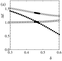
Figure 7: An example of the determination of the $XY$-trivial phase transition point in Fig.4, where $\Delta=1$, $D_{2}=1$ and $D_{4}=0$. In (a), open squares, closed circles and open circles represent, respectively, $\Delta E_{02}^{\rm PBC}(N)$, $\Delta E_{00}^{\rm T-P}(N,+1)$ and $\Delta E_{00}^{\rm T-P}(N,-1)$, where $N=12$. From the crossing point of two curves with open squares and closed circles, we obtain $\delta^{\rm(cr)}(N=12)=0.462647$. In (b), we show the extrapolation of $\delta^{\rm(cr)}(N)$ to $N\to\infty$, supposing that $\delta^{\rm(cr)}(N)$ is a quadratic function of $1/N^{2}$. The broken line represents the least square result by use of $N=6,8,10$ and 12 data, whereas the solid line represent that without $N=6$ data. Both lines almost overlap with each other.

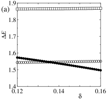
Figure 8: An example of the determination of the SPT-trivial phase transition point in Fig.6 in case of $\Delta=2.2$, $D_{2}=1.5$ and $D_{4}=0.3$. The meanings of symbols and lines are the same as those in Fig.7. From the crossing point of two curves with open circles and closed circles in (a), we obtain $\delta^{\rm(cr)}(N=12)=0.135395$.

Both of the Néel-trivial phase transition and the Néel-SPT phase transition are of the 2D Ising type. We note that the Néel state is a doubly degenerate gapped state, while the trivial state and the SPT state are unique gapped states. For determining the 2D Ising phase transition points, the phenomenological renormalization group (PRG) method[20] is useful. Namely, for instance, running $D_{4}$ with fixing the parameters $\Delta,\delta$ and $D_{2}$, we have numerically solved the PRG equation

$$N\Delta E_{00}^{\rm PBC}(N)=(N+2)\Delta E_{00}^{\rm PBC}(N+2)\\$$ (7)

to obtain the finite-size critical value $D_{4}^{\rm cr}(N+1)$ for given $\Delta,\delta$ and $D_{2}$, where $E_{00}^{\rm PBC}(N)$ is defined by

$$\Delta E_{00}^{\rm PBC}(N)\equiv E_{1}(N,0;{\rm PBC})-E_{0}(N,0;{\rm PBC}).$$ (8)

Then, we have estimated the critical value $D_{4}^{\rm(cr)}$ by taking the $N\to\infty$ limit, assuming that the $N$-dependence of $D_{4}^{\rm(cr)}(N+1)$ is a quadratic function of $1/(N+1)^{2}$. Figure 9 shows an example of determining the Néel-SPT phase transition point in Fig.6 in case of $\Delta=2.2$, $D_{2}=1.5$ and $\delta=0.3$. From Fig.9(b), we estimate $D_{4}^{\rm(cr)}=-0.0244\pm 0.0001$.

Figure 9: An example of the determination of the Néel-SPT phase transition point in Fig.6. In (a), open circles and closed circles represent $N=10$ and $N=12$ points, respectively. We choose $\Delta=2.2$, $D_{2}=1.5$ and $\delta=0.3$. From the crossing point of two curves, we obtain $D_{4}^{\rm(cr)}(N+1=11)=-0.025023$. In (b), the broken line represents the least squares result by use of $N+1=5,7,9$ and 11 data, while the solid line that without $N+1=5$ data.

Here we explain the reason why we have introduced the $D_{4}$ term to obtain the GS phase diagram of Fig.6, where the ID state and the Dim1 state are directly connected. Figure 10 show the GS phase diagram on the $D_{2}-D_{4}$ plane in case of $\Delta=2.2$ and $\delta=0$. For instance, the ID region exists for $1.7917<D_{2}<1.8473$ when $D_{4}=0$, while it exists for $0.5188<D_{2}<1.8984$ when $D_{4}=0.2$. We can see that the positive $D_{4}$ considerably widens the ID region, as we have already pointed out in Ref.oka3. Thus, the introduction of the $D_{4}$ term is very crucial to obtain the GS phase diagram in which the ID state and the Dim1 state are directly connected. We note that the addition of the $D_{4}$ term does not change any symmetry of the Hamiltonian without the $D_{4}$ term.

Figure 10 also well explains the difference between our[1, 2, 3] and Tzeng’s[12] conclusion and Kjäll et al.’s[13] one with respect to the existence of the ID phase on the $\Delta-D_{2}$ plane in case of $D_{4}=\delta=0$, which we already stated. The $D_{4}$ coordinate of the point A in Fig.10(b) is $D_{4}^{\rm(A)}=-0.0005\pm 0.0001$, where A is the bottom of the ID region. We believe that our result is correct, but it is possible that a very small upward shift of the point A by $\Delta D_{4}^{\rm(A)}=0.0005$ (or larger) obtained by other methods brings about the absence of the ID region on the $\Delta-D_{2}$ plane with $D_{4}=\delta=0$. Since the fact that $D_{4}^{\rm(A)}$ is very near to $D_{4}=0$ seems to be accidental, we think that the above difference is not a serious problem.

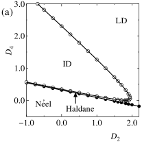
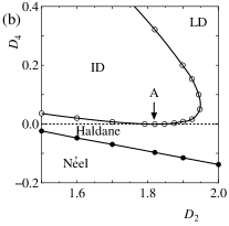
Figure 10: GS phase diagram on the $D_{2}-D_{4}$ plane in case of $\Delta=2.2$ and $\delta=0$. (a) is for a wider region, and (b) is an enlarged view near the bottom of the ID region. In (b), the point A shows the bottom of the ID region, the $D_{4}$ coordinate of which is $D_{4}=-0.0005\pm 0.0001$. The horizontal broken line shows $D_{4}=0$.

Finally we shortly mention the $S=1$ case. Tonegawa et al.[21] and Chen et al.[22] investigated the GS phase diagram of the bond alternating $S=1$ quantum spin chain with the on-site anisotropy described by

$${\mathcal{H}}_{4}=\sum_{j}[1+(-1)^{j}\delta]{\mbox{\boldmath$S$}}_{j}\cdot{\mbox{\boldmath$S$}}_{j+1}+D_{2}\sum_{j}(S_{j}^{z})^{2},~{}~{}~{}~{}S=1.$$ (9)

They obtained the GS phase diagram on the $\delta-D_{2}$ plane and showed that the LD state and the dimer state belong to the same phase. We note that, for the $S=1$ case, the Haldane state is the SPT state, and the LD state and the dimer state are the trivial states.

In conclusion, employing the LS and PRG analysis based on the exact diagonalization calculation, we have determined the GS phase diagrams of Hamiltonian (3) on the $\delta-D_{2}$ plane for the $(\Delta,D_{4})=(1,0)$ case (Fig.4) and the $(\Delta,D_{4})=(2.2,0)$ case (Fig.5), and on the $\delta-D_{4}$ plane for the $(\Delta,D_{2})=(2.2,1.5)$ case (Fig.6). We have proved that the Haldane state, the LD state and the Dim2 states belong to the same trivial phase by showing the existence of adiabatic paths directly connecting these states without the quantum phase transition. In a similar way, we have proved that the ID state and the Dim1 state belong to the same SPT phase.

We would like to express our appreciation to Masaki Oshikawa and Shunsuke C. Furuya for stimulating discussions. We thank the Supercomputer Center, Institute for Solid State Physics, University of Tokyo, and the Computer Room, Yukawa Institute for Theoretical Physics, Kyoto University, for computational facilities.

References

- [1] T. Tonegawa, K. Okamoto, H. Nakano, T. Sakai, K. Nomura, and M. Kaburagi: J. Phys. Soc. Jpn. 80, 043001 (2011).
- [2] K. Okamoto, T. Tonegawa, H. Nakano, T. Sakai, K. Nomura, and M. Kaburagi: J. Phys.: Conf. Ser. 302, 012014 (2011).
- [3] K. Okamoto, T. Tonegawa, H. Nakano, T. Sakai, K. Nomura, and M. Kaburagi: J. Phys.: Conf. Ser. 320, 012018 (2011).
- [4] K. Okamoto, T. Tonegawa, T. Sakai, and M. Kaburagi: JPS Conf. Proc. 3, 014022 (2014).
- [5] K. Okamoto and K. Nomura: Phys. Lett. A 169, 433 (1992).
- [6] K. Nomura and K. Okamoto: J. Phys. A: Math. Gen. 27, 5773 (1994).
- [7] A. Kitazawa: J. Phys. A: Math. Gen. 30, L285 (1997).
- [8] K. Nomura and A. Kitazawa: J. Phys. A: Math. Gen. 31, 7341 (1998)
- [9] M. Oshikawa: J. Phys.: Condens. Matter 4, 7469 (1992).
- [10] F. Pollmann, A. M. Turner, E. Berg, and M. Oshikawa: Phys. Rev. B 81, 064439 (2010).
- [11] F. Pollmann, E. Berg, A. M. Turner, and M. Oshikawa: Phys. Rev. B 85, 075125 (2012).
- [12] Y.-C. Tzeng: Phys. Rev. B 86, 024403 (2012).
- [13] J. A. Kjäll, M. P. Zaletel, R. S. K. Mong, J. H. Bardarson, and F. Pollmann: Phys. Rev. B 87, 235106 (2013).
- [14] M. Yamanaka, M. Oshikawa, and S. Miyashita: J. Phys. Soc. Jpn. 65, 1562 (1996).
- [15] S. Yamamoto: Phys. Rev. 55, 3603 (1997).
- [16] A. Kitazawa and K. Nomura: J. Phys. Soc. Jpn. 66, 3379 (1997).
- [17] M. Nakamura and S. Todo: Phys. Rev. Lett. 89, 077204 (2002).
- [18] Z. L. Berezinskii: Sov. Phys. JETP 34, 610 (1971).
- [19] J. M. Kosterlitz and D. J. Thouless: J. Phys. C 6, 1181 (1973).
- [20] M. P. Nightingale: Physica A 83, 561 (1976).
- [21] T. Tonegawa, T. Nakao, and M. Kaburagi: J. Phys. Soc. Jpn. 65, 3317 (1996).
- [22] W. Chen, K. Hida, and B. C. Sanctuary: J. Phys. Soc. Jpn. 69, 237 (2000).