Numerical multi-loop integrals and applications

Abstract

Higher-order radiative corrections play an important role in precision studies of the electroweak and Higgs sector, as well as for the detailed understanding of large backgrounds to new physics searches. For corrections beyond the one-loop level and involving many independent mass and momentum scales, it is in general not possible to find analytic results, so that one needs to resort to numerical methods instead. This article presents an overview of a variety of numerical loop integration techniques, highlighting their range of applicability, suitability for automatization, and numerical precision and stability.

In a second part of this article, the application of numerical loop integration methods in the area of electroweak precision tests is illustrated. Numerical methods were essential for obtaining full two-loop predictions for the most important precision observables within the Standard Model. The theoretical foundations for these corrections will be described in some detail, including aspects of the renormalization, resummation of leading log contributions, and the evaluation of the theory uncertainty from missing higher orders.

1 Introduction

With high-statistics data from LEP, SLC, Tevatron, LHC, B factories, and other experiments, particle physics has forcefully moved into the precision realm during the last few decades. Due to the small uncertainties of many experimental results, it is possible to test the Standard Model at the quantum level and to put stringent indirect constraints on new physics beyond the Standard Model. In particular, electroweak precision tests put lower bounds on generic heavy new physics of several TeV [1]. Due to the level of precision, the inclusion of radiative corrections has become an integral part in the analysis and interpretation of experimental results.

In many cases, the dominant corrections arise from QED or QCD contributions due to the radiation of photons, gluons or other massless partons from the initial or final legs of a scattering or decay process. These can amount to tens of percent or more in some situations. However, for observables with percent-level or better precision, electroweak corrections also become relevant. With increasing order in perturbation theory and increasing number of independent mass and momentum scales, it becomes more difficult to find analytical solutions to the virtual radiative corrections. This problem is particularly acute for electroweak corrections, which involve many particles with different, non-negligible masses. Consequently, in these situations it becomes more convenient or even necessary to consider numerical techniques.

This review presents an overview of numerical integration techniques, which are primarily used for the calculations of electroweak loop corrections. The advantages and disadvantages of the different methods are outlined, elucidating that there is no single technique that works best in all circumstances. In a second part, the application of these methods for the calculation of two-loop corrections to electroweak precision observables is discussed, and the phenomenological role of these corrections in precision tests of the Standard Model is elucidated.

A “Feynman integral” is obtained from diagrams or amplitudes that contain one or more closed loops in the corresponding Feynman graph. The momentum flowing through the loop $i$, denoted $q_{i}$, is not constrained by energy-momentum conservation and thus must be integrated over, $\int d^{4}q_{i}/(i\pi^{2})\dots$ In general, these loop integrals are divergent. One class of divergences, called ultraviolet (UV) singularities, are associated with the limit $|q_{i}|\to\infty$. These are removed through the renormalization of couplings, masses and the wave function of the incoming and outgoing fields of a given physical process. A second class of divergences, called infrared singularities (IR), can be divided into two types: soft and collinear singularities. The former can occur when the momentum of a massless propagator inside the loop tends to zero, while the latter can appear if the momentum of a massless loop propagator becomes collinear with an external light-like momentum that connects to one end of this propagator. Soft and final-state collinear singularities cancel when the virtual loop corrections are combined with real emission contributions.

Nevertheless, UV and IR singularities in individual loop amplitudes must be regulated before they can be canceled. Throughout this article, dimensional regularization [2] is employed. Within dimensional regularization, the space-dimension is analytically continued from 4 to an arbitrary number $D=4-2\epsilon$. The UV and IR singularities are then manifested terms with $1/\epsilon^{n}$ poles when taking the limit $\epsilon\to 0$.

For a physical observable, after summing over unobserved polarizations, a $L$-loop integral in dimensional regularization can be written in the following generic form:

$$I=\int{\mathfrak{D}}q_{1}\cdots{\mathfrak{D}}q_{L}\;\frac{(q_{i_{1}}\cdot p_{j_{1}})(q_{i_{2}}\cdot p_{j_{2}})\cdots}{D_{1}^{\nu_{1}}\cdots D_{n}^{\nu_{n}}}\,,$$ (1)

$${\mathfrak{D}}q_{i}=\frac{d^{D}q_{i}}{i\pi^{D/2}},\qquad\qquad D_{j}=k_{j}^{2}-m_{j}^{2},$$ (2)

where the $k_{j}$ are linear combinations of one or more loop momenta $q_{1},\,q_{2},\,\dots$ and zero or more external momenta $p_{1},\,p_{2},\,\dots$, while $m_{j}$ are the masses of the internal propagators, and $\nu_{j}$ are integer numbers. Note that here and for the rest of this article, the Feynman $i\varepsilon$ prescription is implicitly assumed, $D_{j}=k_{j}^{2}-m_{j}^{2}\to k_{j}^{2}-m_{j}^{2}+i\varepsilon$. In other words, the propagator momentum $k_{j}$ is supposed to be endowed with an infinitesimal imaginary part. Integrals with non-trivial numerator terms in eq. (1) are often called “tensor integrals” since they can be written as

$$I =p_{j_{1}}^{\mu_{1}}p_{j_{2}}^{\mu_{2}}\cdots\int{\mathfrak{D}}q_{1}\cdots{\mathfrak{D}}q_{L}\;\frac{q_{i_{1},\mu_{1}}q_{i_{2},\mu_{2}}\cdots}{D_{1}^{\nu_{1}}\cdots D_{n}^{\nu_{n}}}\,.$$ (3)

A helpful and widely used tool for the analysis of Feynman integrals is the Feynman parametrization. With its help, an integral of the form in eq. (1) without numerator terms turns into

$$I=\int\frac{{\mathfrak{D}}q_{1}\cdots{\mathfrak{D}}q_{L}}{D_{1}^{\nu_{1}}\cdots D_{n}^{\nu_{n}}}=\frac{\Gamma(N)}{\Gamma(\nu_{1})\cdots\Gamma(\nu_{n})}\int_{0}^{1}dx_{1}\cdots dx_{n}\;\delta\Bigl{(}1-\sum_{i=1}^{n}x_{i}\Bigr{)}\int{\mathfrak{D}}q_{1}\cdots{\mathfrak{D}}q_{L}\;\frac{x_{1}^{\nu_{1}-1}\cdots x_{n}^{\nu_{n}-1}}{[x_{1}D_{1}+\ldots+x_{n}D_{n}]^{N}},$$ (4)

where $N=\nu_{1}+...+\nu_{n}$. The denominator sum can be written as

$$x_{1}D_{1}+\ldots+x_{n}D_{n}=\sum_{i,j=1}^{L}A_{ij}q_{i}\cdot q_{j}-2\sum_{i=1}^{L}q_{i}\cdot P_{i}-M,$$ (5)

where the $(L{\times}L)$-matrix $A$, the $L$-column vector $P$, and the scalar function $M$ depend on the Feynman parameters $x_{i}$. Upon shifting the loop momenta to remove the linear term and carrying out the loop integration, the integral becomes

$$I =\frac{(-1)^{N}\,\Gamma(N-LD/2)}{\Gamma(\nu_{1})\cdots\Gamma(\nu_{n})}\int_{0}^{1}dx_{1}\cdots dx_{n}\;\delta\Bigl{(}1-\sum_{i=1}^{n}x_{i}\Bigr{)}\;x_{1}^{\nu_{1}-1}\cdots x_{n}^{\nu_{n}-1}\,\frac{{\cal U}^{N-(L+1)D/2}}{{\cal V}^{N-LD/2}},$$ (6)

with

$${\cal U} =\det(A),\qquad\qquad{\cal V}=\det(A)\,\Bigl{[}M+\sum_{i,j=1}^{L}A^{-1}_{ij}\,P_{i}\cdot P_{j}\Bigr{]}.$$ (7)

Instead of introducing Feynman parameters for all $L$ loop integrations at once, as in (4), one can alternatively introduce them loop by loop, which is advantageous for some applications discussed in this review.

Besides using Feynman parameters, another useful representation of Feynman integrals is obtained from the use of so-called Schwinger or alpha parameters. In fact, the alpha parametrization is closely related to the Feynman parametrization; see chapter 2.3 of Ref. [31] for more information.

1.1 Analytic methods

From a historical perspective, the default approach to loop calculations is the use of analytical methods. This procedure can be divided into two steps: (a) reduction of the complete lists of loop integrals for a given physical process to a small set of scalar “master integrals”; and (b) evaluation of the master integrals in terms of analytical functions that depend on the propagator masses, invariants of the external momenta, and the integration dimension $D$. In practice, it is usually sufficient to carry out the last step as an expansion in $\epsilon=2/(4-D)$, dropping all terms $\epsilon^{n}$ with powers $n>0$.

The reduction to master integrals can be achieved through a number of different methods:

• The Passarino-Veltman approach [3], which is based on the decomposition of integrals with different terms in the numerator of (1) into Lorentz covariant monomials: This technique is applicable to generic one-loop integrals, and it has been extended for some classes of two-loop integrals [4], but it does not work for arbitrary multi-loop integrals.

• Integration-by-parts relations [5]: In dimensional regularization, these take the form

  $$\int\prod_{l=1}^{L}{\mathfrak{D}}q_{l}\,\partial q_{i}^{\mu}\,k_{j,\mu}\,F(\{q_{k}\},\{p_{m}\},\{m_{n}\})=\oint dS^{\mu}_{q_{i}}\int\prod_{l\neq i}{\mathfrak{D}}q_{l}\,k_{j,\mu}\,F(\{q_{k}\},\{p_{m}\},\{m_{n}\})=0,$$ (8)

  where $k_{j}$ may be loop or external momentum and $F$ is an expression containing propagators and dot products of momenta, but no free Lorentz indices. The surface integral on the right-hand side of (8) extends over the boundary of the $D$-dimensional integration volume of the loop momentum $q_{i}$, and it vanishes in dimensional regularization. On the other hand, when evaluating the derivative on the left-hand side, one obtains a linear relation between different integrals of the form (1). By considering different choices for $q_{i}$, $k_{j}$ and $F$ one can generate a large, overconstrained linear equation system, which can be solved to find how a complicated loop integral can be expressed as a linear combination of simpler master integrals.

  This approach is very suitable for the automated implementation in computer algebra systems. The first such computer program was MINCER [8], which was developed for the reduction of 3-loop massless propagator diagrams. A systematic prescription for building and solving such linear equation systems for arbitrary multi-loop integrals was presented in Refs. [6] and is usually referred to as the “Laporta algorithm”. The integration-by-parts identities can be supplemented by Lorentz invariance identities [7] to arrive at a more economical system of equations. Today, several public codes are available that can perform the reduction of general multi-loop integrals, such as AIR [9], FIRE [10], Reduze [11], LiteRED [12]. These programs take advantage of integration-by-parts and Lorentz invariance identities together with symmetry properties of the integrals and advanced linear reduction algorithms.

  Instead of solving the system of integration-by-parts identities through the “Laporta algorithm”, an alternative method for vacuum integrals has been presented by Baikov [13]. This technique allows one to directly determine the coefficients $c_{k}$ in the reduction of a Feynman integral $I$, $I=\sum_{k}c_{k}\,I^{0}_{k},$ where $I^{0}_{k}$ are the master integrals. It was shown in Ref. [13] that the integration-by-parts identities can be transformed into differential equations, for which an explicit solution in terms of the masses $m_{ij}$ and propagator indices $\nu_{j}$ of the original integral can be found. This method can also be used for integrals with external momenta by relating them to vacuum integrals with additional propagators. The idea’s from Baikov’s method can also be used to find a suitable basis of master integrals [14].

• Tensor reduction through tensor operators [15, 16]: In Ref. [15] it was shown that integrals with non-trivial numerator terms can be written as a tensor operator acting on a scalar integral with numerator 1. The proof follows from a careful examination of the Schwinger parametrization of the tensor integrals. The result of the action of the tensor operator are scalar integrals with higher powers of propagators in the denominator and/or shifted space-time dimension $D+2,\,D+4\,\dots$ Integrals with shifted dimension can be related to $D$-dimensional scalar integrals by using a variant of the tensor operator mentioned above. Scalar integrals with higher powers of propagators can then be reduced to the master integrals by the integration-by-parts identities as described in the previous bullet [15, 16].

• Unitarity-based methods, which are founded on the basic tenet of the optical theorem that the sum of all diagrams contributing to a certain process is related to the discontinuities of the amplitude across its branch cuts: By introducing the concepts of generalized cuts and the on-shell singularity structure of loop amplitudes [17], it has become feasible to reduce a general one-loop diagram to master integrals by analyzing the residues of these singularities [18].

  These methods are very powerful for the computation of multi-leg one-loop processes, and the implementation of automated algorithms into computer codes has been achieved by several groups [19]. For a recent review on this topic, see $e.\,g.$ Ref. [20]. The extension of the unitarity-based approach to higher loop orders is more difficult, but notable advances have been made (see $e.\,g.$ Ref. [21]).

For the analytic calculation of multi-loop master integrals, a variety of different techniques have been developed:

• Direct integration over Feynman parameters, starting from the expression (6), is the most straightforward method for evaluating master integrals. For more complicated Feynman integrals, the last few Feynman parameter integrations are typically only possible after expanding in powers of $\epsilon=2/(4-D)$. This method has been used, for example, for two-loop vertex corrections with massless propagators [22], massive two-loop diagrams at threshold [23], and massive three-loop vacuum integrals [24]. By integrating over Schwinger instead of Feynman parameters, it is possible to evaluate certain more difficult cases with more than three loops and multiple independent scales, see $e.\,g.$ Ref. [25]. However, the parametric integration approach reaches a limit for general multi-loop diagrams with several independent scales.

• Mellin-Barnes representations are very useful for further processing of difficult Feynman parameter or alpha parameter integrals. The key idea is to replace the sum in the denominator of a Feynman parameter or alpha parameter integral by the Mellin-Barnes integral

  $$\frac{1}{(A_{0}+\ldots+A_{m})^{Z}}=\frac{1}{(2\pi i)^{m}}\int_{{\cal C}_{1}}dz_{1}\cdots \int_{{\cal C}_{m}}dz_{m}\;A_{1}^{z_{1}}\cdots A_{m}^{z_{m}}A_{0}^{-Z-z_{1}-\ldots-z_{m}}$$ (9)

  $$\times\frac{\Gamma(-z_{1})\cdots\Gamma(-z_{m})\Gamma(Z+z_{1}+\ldots+z_{m})}{\Gamma(Z)}$$

  where the integration contours ${\cal C}_{i}$ for $z_{i}$ are straight lines parallel to the imaginary axis chosen such that all arguments of the gamma functions have positive real parts. This representation is very convenient for the isolation of singularities in $\epsilon$ (see section 2.3 for more details). After carrying out the Feynman or alpha parameter integrals, the Mellin-Barnes integration can be performed by closing the integration contours in the complex plane and summing up the residues. This technique has been used for the calculation of various two- and three-loop master integrals, see for instance Refs. [26, 27, 28].

• The differential equation method [29] has been used widely for the evaluation of master integrals beyond one-loop order. The basic idea is to take derivatives of a given master integral $I_{k}^{0}$ with respect to a kinematical invariant or mass. The result of this differentiation on the integrand of $I_{k}^{0}$ produces a different Feynman integral, which in general is non-minimal but can be reduced to a linear combination of master integrals by using, for example, integration-by-parts identities. Thus one obtains a differential equation of the form

  $$\frac{\partial}{\partial(m_{i}^{2})}I_{k}^{0} =\sum_{l}f_{kl}(\{m_{n}\},\{s_{pr}\},D)\,I^{0}_{l}$$ (10)

  or

  $$\frac{\partial}{\partial s_{ij}}I_{k}^{0} =\sum_{l}f^{\prime}_{kl}(\{m_{n}\},\{s_{pr}\},D)\,I^{0}_{l},$$ (11)

  where the coefficient functions $f_{kl}$ depend on the masses $m_{n}$ and kinematical invariants $s_{pr}=(p_{p}+p_{r})^{2}$ of the integrals, as well as the dimension $D$. By organizing the differential equations appropriately, one can make sure that the right-hand side of (10),(11) contains only $I_{k}^{0}$ itself and simpler master integrals, whose solution is assumed to be known already. A good choice of the basis of master integrals $\{I_{k}^{0}\}$ is essential in this context [30]. Then the system of differential equations can be solved sequentially to obtain solutions for all masters. In practice, it is often difficult to find analytical solutions for arbitrary dimension $D$, in which case one can instead expand both sides of the differential equation in powers of $\epsilon=2/(4-D)$ and then construct the solution order by order in $\epsilon$.

A more detailed exposition of analytic loop calculation methods can be found $e.\,g.$ in Ref. [31].

Analytical methods work well for problems with few independent momentum and mass scales, leading to compact results suitable for fast evaluation in Monte-Carlo event generators. However, for multi-scale problems, both of the main steps of the analytical approach run into difficulties. The reduction to master integrals requires significantly larger computing resources and leads to large and unwieldy expressions. Furthermore, master integrals with many independent momentum and mass scales can typically not be solved in terms of known elementary functions. This can be circumvented to some extent by introducing new types of functions, such as harmonic polylogarithms [32] and Goncharov polylogarithms [33], but it is unclear if these concepts can be extended to arbitrary Feynman integrals.

In the following two subsections, the two main philosophies for moving beyond the limitations of the analytical approach are outlined.

1.2 Asymptotic expansions

In the presence of a suitable small expansion parameter, for example the ratio $m/M$ of a small mass $m$ and a large mass $M$, a difficult multi-scale Feynman diagram may be expanded in powers of this small parameter. The coefficients of this expansion are diagrams with fewer scales and/or fewer loops, which are simpler to evaluate analytically. This procedure, called “asymptotic expansion”, is an extension of Taylor expansions which can contain non-analytical functions of the small parameter, such a logarithms.

Typically, a small expansion parameter is obtained if one of the masses or momenta in a given problem are significantly larger ($e.\,g.$ the top-quark mass in the Standard Model or the beam energy of a high-energy collider) or smaller ($e.\,g.$ the charm-quark mass in B-meson decays) than other relevant scales. In some cases, the small parameter could also be the difference between two masses and/or momenta. In some cases, even an expansion parameter of magnitude close to 1 leads to satisfactory results (see $e.\,g.$ Ref. [26]). For many applications, the first few terms in an asymptotic expansion are sufficient to achieve the desired precision of the result.

The general prescription for the asymptotic expansion in the presence of a large scale $\Lambda$ is [34]

$$\Gamma(\Lambda,\{m_{i}\},\{p_{j}\})=\sum_{\gamma}\Gamma{/}\gamma(\{m_{i}\},\{p_{j}\})\star T_{\{m_{i}\},\{p_{j}\}}\,\gamma(\Lambda,\{m_{i}\},\{p_{j}\}).$$ (12)

Here $\Lambda\gg m_{i},p_{j}$ is a momentum or mass that is significantly larger than the collection of other masses, $\{m_{i}\}$, and momenta, $\{p_{j}\}$. $\Gamma$ is the Feynman diagram under consideration, and the sum runs over all subgraphs $\gamma$ of $\Gamma$ that contain all vertices and propagators where $\Lambda$ appears. The subgraphs also must be one-particle irreducible in their connected parts. $\Gamma{/}\gamma\star T_{\{m_{i}\},\{p_{j}\}}\gamma$ denotes that the integrand of the subgraph $\gamma$ of $\Gamma$ is replaced by its Taylor expansion with respect to all small masses and external momenta. In particular, the loop momenta of $\Gamma$ that are external to $\gamma$ also have to be treated as small.

The major advantage of this method is that the expansion in the small parameter is carried out in the integrand, before any loop integral is evaluated, and thus leads to simpler integrals than the original problem. It can be shown that this produces correct results by using the “strategy of regions” [36, 35]. This technique subdivides the integration space into regions where the different loop momenta are large or small. The “strategy of regions” also allows one to tackle other cases than simple large or small mass and momentum expansions, such as threshold expansions [35] or mass difference expansions [37].

The method of asymptotic expansions fails if an internal threshold of the loop diagram is crossed when taking the limit of the small expansion parameter. Furthermore, while asymptotic expansions typically lead to fairly compact final results, one has to deal with large and unwieldy expressions during intermediate steps, especially in the case of multiple expansions. Also, in the case of multiple expansions, more terms may be needed to achieve satisfactory precision.

1.3 Numerical integration

Instead of trying to obtain a final result in terms of an analytical formula, one can alternatively perform at least some of the integrations for a loop diagram numerically. While in principle the numerical integrations can be carried out directly in the space of the loop momenta $q_{i}$ in (1), it is typically more convenient to switch to different variables, such as Feynman parameters, Mellin-Barnes integrals, and other options that will be discussed in the following chapter.

The advantage of the numerical integration approach is that, at least conceptually, it poses no limit to the number of different propagators and mass and momentum scales present in a loop diagram. Thus it is particularly suitable for the calculation of multi-loop corrections in the full Standard Model. However, there are other difficulties encountered by numerical loop integration techniques:

Isolation of UV and IR singularities:

Physical amplitudes can exhibit UV and IR (soft and collinear) divergences, which appear as $1/\epsilon$ poles in dimensional regularization. These need to be identified and extracted before the numerical integration can be performed. Ideally one would like an algorithmic prescription for this step, which can be implemented in a computer algebra system and works automatically for a large class of Feynman diagrams. For the case of QED (as opposed to non-Abelian theories like QCD), the IR divergences may also be regulated by a small photon mass, which does not require any specific treatment before the numerical evaluation. On the other hand, a photon mass that is much smaller than other mass and momentum scales may pose a challenge to the convergence and precision of the numerical integrator.

Stability and convergence:

For a numerical integration technique to be practical, it must be able to produce a sufficiently precise result with a reasonable number of integrand evaluation points. The precision should improve in a predictable manner when the number of integration points is increased. Typically, these requirements can be satisfied if the numerical integration volume is of relatively low dimension, or if the integrand is ensured to be relatively smooth, without large peaks or oscillatory behavior. In the former case, it is typically advantageous to use standard discrete integration algorithms, whereas the latter case is suitable for Monte-Carlo and Quasi-Monte-Carlo integration routines.

A particular difficult situation is the occurrence of local singularities that are formally integrable, but which cannot be handled by standard numerical integration routines. Such singularities usually originate from internal thresholds of a loop diagram, $i.\,e.$ if a Feynman diagram has physical cuts that meet the condition $0<\sum_{i\in\rm cut}m_{i}<\sqrt{p^{2}_{\rm tot,cut}}$, where the sum runs over the masses of the cut propagators and $p_{\rm tot,cut}$ is the total momentum flowing through the cut. These singularities are typically located in the inner part of the integration domain ($i.\,e.$ not on its boundary), and their impact needs to be mitigated through a suitable change of integration variables or some manipulation of the integrand.

Generality:

A numerical loop integration method should preferably be applicable to a large class of Feynman diagrams, without special techniques for each different diagram topology. Obviously, this is already a problem for analytical methods, and in fact numerical integration approaches have the potential to be superior in this aspect.

In the following, some of the most commonly used and powerful numerical integration techniques will be discussed in more detail. At the end of the next chapter, their strengths and weaknesses with respect to the aforementioned three criteria will be summarized.

2 Numerical integration techniques

2.1 Feynman parameter integration of massive two-loop integrals

A general method for the numerical evaluation of massive two-loop diagrams was introduced in Refs. [38, 39]. Let us consider an arbitrary $N$-propagator two-loop integral

$$I_{(2)}=\int{\mathfrak{D}}q_{1}{\mathfrak{D}}q_{2}\;N(q_{1},q_{2},\{p_{i}\})\begin{aligned} &\times\frac{1}{[(q_{1}+p_{1})^{2}-m_{1}^{2}]\cdots[(q_{1}+p_{n})^{2}-m_{n}^{2}]}\\ &\times\frac{1}{[(q_{2}+p_{n+1})^{2}-m_{n+1}^{2}]\cdots[(q_{1}+p_{n+m})^{2}-m_{n+m}^{2}]}\\ &\times\frac{1}{[(q_{1}+q_{2}+p_{n+m+1})^{2}-m_{n+m+1}^{2}]\cdots[(q_{1}+q_{2}+p_{N})^{2}-m_{N}^{2}]},\end{aligned}$$ (13)

where $p_{1},\dots,p_{N}$ are external momenta, some of which may be zero or linearly dependent on other momenta, and $N$ is a polynomial function of loop and external momenta. As a first step, three sets of Feynman parameters are introduced, one set each for all propagators with loop momentum $q_{1}$, $q_{2}$ and $q_{1}+q_{2}$, respectively. After shifting the loop momenta, one thus can write (13) in the form

$$I_{(2)}=\int_{0}^{1}dx_{1}\cdots dx_{N-3}\int{\mathfrak{D}}q_{1}{\mathfrak{D}}q_{2}\;\frac{\tilde{N}(q_{1},q_{2},\{p_{i}\})}{[q_{1}^{2}-\tilde{m}_{1}^{2}]^{\nu_{1}}[q_{2}^{2}-\tilde{m}_{2}^{2}]^{\nu_{2}}[(q_{1}+q_{2}+\tilde{p})^{2}-\tilde{m}_{3}^{2}]^{\nu_{3}}}.$$ (14)

Here $\tilde{p}$ is a linear combination of the external momenta $p_{i}$, which depends on the Feynman parameters $x_{j}$, and $\tilde{m}_{1,2,3}$ are functions of the masses and momenta in (13) and of the Feynman parameters.

Using a decomposition of the $q_{1,2}$-dependent terms in the numerator into parts that are transverse and longitudinal with respect to $\tilde{p}$ [39], one finds that all such integrals can be reduced to scalar integrals of the form

$$I_{(2)} =\int_{0}^{1}dx_{1}\cdots dx_{N-3}\;{\cal P}^{ab}_{\nu_{1}\nu_{2}\nu_{3}}(\tilde{m}_{1},\tilde{m}_{2},\tilde{m}_{3};\tilde{p}^{2}),$$ (15)

$${\cal P}^{ab}_{\nu_{1}\nu_{2}\nu_{3}}(\tilde{m}_{1},\tilde{m}_{2},\tilde{m}_{3};\tilde{p}^{2}) =\int{\mathfrak{D}}q_{1}{\mathfrak{D}}q_{2}\;\frac{(q_{1}\cdot p)^{a}(q_{2}\cdot p)^{b}}{[q_{1}^{2}-\tilde{m}_{1}^{2}]^{\nu_{1}}[q_{2}^{2}-\tilde{m}_{2}^{2}]^{\nu_{2}}[(q_{1}+q_{2}+p)^{2}-\tilde{m}_{3}^{2}]^{\nu_{3}}}.$$ (16)

Scalar integrals ${\cal P}^{ab}_{\nu_{1}\nu_{2}\nu_{3}}$ with different indices can be related by considering derivatives with respect to its mass and momentum arguments, leading to

$${\cal P}^{ab}_{\nu_{1}+1,\nu_{2},\nu_{3}} =-\frac{1}{\nu_{1}}\,\frac{\partial}{\partial(\tilde{m}_{1}^{2})}{\cal P}^{ab}_{\nu_{1}\nu_{2}\nu_{3}},$$ (17)

$${\cal P}^{a+1,b}_{\nu_{1}+1,\nu_{2},\nu_{3}} =\frac{1}{2\nu_{1}}\Bigl{[}2\tilde{p}^{2}\frac{\partial}{\partial(\tilde{p}^{2})}-(a+b)\Bigr{]}{\cal P}^{ab}_{\nu_{1}\nu_{2}\nu_{3}}+\frac{a\tilde{p}^{2}}{2\nu_{1}}{\cal P}^{a-1,b}_{\nu_{1}\nu_{2}\nu_{3}},$$ (18)

$${\cal P}^{a,b+1}_{\nu_{1},\nu_{2}+1,\nu_{3}} =\frac{1}{2\nu_{2}}\Bigl{[}2\tilde{p}^{2}\frac{\partial}{\partial(\tilde{p}^{2})}-(a+b)\Bigr{]}{\cal P}^{ab}_{\nu_{1}\nu_{2}\nu_{3}}+\frac{b\tilde{p}^{2}}{2\nu_{2}}{\cal P}^{a,b-1}_{\nu_{1}\nu_{2}\nu_{3}}.$$ (19)

Using the relations, one can express all loop functions ${\cal P}^{ab}_{\nu_{1}\nu_{2}\nu_{3}}$ in terms of a minimal set, for which the authors of Ref. [39] chose the following ten: ${\cal P}^{00}_{211}$, ${\cal P}^{10}_{211}$, ${\cal P}^{01}_{211}$, ${\cal P}^{20}_{211}$, ${\cal P}^{11}_{211}$, ${\cal P}^{02}_{211}$, ${\cal P}^{30}_{211}$, ${\cal P}^{21}_{211}$, ${\cal P}^{12}_{211}$, ${\cal P}^{03}_{211}$. This set is a suitable choice for all renormalizable theories, but note that not all of these ten functions are independent.

The UV-divergent part of the ten master functions can be evaluated analytically, while their finite parts can be expressed in terms of one-dimensional integral representations [39]. For example, introducing two Feynman parameters to combine the three propagators into one, expanding in $\epsilon$, and integrating over one Feynman parameter, one finds for the function ${\cal P}^{00}_{211}$ [38]:

$${\cal P}^{00}_{211}(\tilde{m}_{1},\tilde{m}_{2},\tilde{m}_{3};\tilde{p}^{2}) =\begin{aligned} &\frac{1}{2\epsilon}+\frac{1}{\epsilon}\biggl{[}\frac{1}{2}-\gamma_{\rm E}-\log\tilde{m}_{1}^{2}\biggr{]}\\ &+\Bigl{(}\frac{1}{2}-\gamma_{\rm E}-\log\tilde{m}_{1}^{2}\Bigr{)}^{2}+\frac{\pi^{2}-9}{12}+g(\tilde{m}_{1},\tilde{m}_{2},\tilde{m}_{3};\tilde{p}^{2}),\end{aligned}$$ (20)

$$g(\tilde{m}_{1},\tilde{m}_{2},\tilde{m}_{3};\tilde{p}^{2}) =\int_{0}^{1}dx\,\biggl{[}{\rm Li}_{2}\Bigl{(}\frac{1}{1-y_{+}}\Bigr{)}+{\rm Li}_{2}\Bigl{(}\frac{1}{1-y_{-}}\Bigr{)}+y_{+}\log\frac{y_{+}}{y_{+}-1}+y_{-}\log\frac{y_{-}}{y_{-}-1}\biggr{]},$$ (21)

$$y_{\pm} =-\frac{1}{2\tilde{p}^{2}}\bigl{[}\tilde{m}_{1}^{2}-\mu^{2}-\tilde{p}^{2}\pm\lambda^{1/2}(\tilde{m}_{1}^{2},\mu^{2},\tilde{p}^{2})\bigr{]},$$ (22)

$$\mu^{2} =\frac{\tilde{m}_{2}^{2}\,x+\tilde{m}_{3}^{2}(1-x)}{x(1-x)},$$ (23)

where $\gamma_{\rm E}\approx 0.577216$ is the Euler number, ${\rm Li}_{2}(z)$ is the dilogarithm or Spence’s function, and

$$\lambda(a,b,c)=a^{2}+b^{2}+c^{2}-2(ab+ac+bc)$$ (24)

is the Källén function. Here it is understood that the usual Feynman $i\varepsilon$ prescription is applied, $i.\,e.$ $\tilde{p}^{2}\to\tilde{p}^{2}+i\varepsilon$.

The integration over the last Feynman parameter $x$, as well as the Feynman parameters introduced in eq. (14), can then be carried out numerically, resulting in a $(N-2)$-dimensional numerical integration.

For $\tilde{p}^{2}>(\tilde{m}_{1}+\tilde{m}_{2}+\tilde{m}_{3})^{2}$ the integrand of (21) (and similarly for the other ${\cal P}^{ab}_{\nu_{1}\nu_{2}\nu_{3}}$ functions) develops singularities at

$$x =\frac{1}{2r^{2}}\bigl{[}-m_{2}^{2}+m_{3}^{2}+r^{2}\pm\lambda^{1/2}(m_{2}^{2},m_{3}^{2},r^{2})\bigr{]}, r^{2} =m_{1}^{2}+\tilde{p}^{2}-2\sqrt{\tilde{p}^{2}}.$$ (25)

These points must be circumvented by deforming the $x$-integration into the complex plane. Similarly, values of the Feynman parameters $x_{1,2,\dots}$ in (14) where $\tilde{m}^{2}_{1,2,3}$ become zero should also be avoided by choosing a complex integration path for these parameters. After this, the integrand is reasonably smooth if all masses and external momentum invariants are of similar order of magnitude, and the numerical integration can be performed with standard discrete (for low dimensionality) or Monte-Carlo (for high dimensionality) integration routines.

A suitable integration path for $x$ is described in Ref. [38], but the choice of complex contour for the other integration variables may depend on the topology of the loop diagram and on the pattern of masses appearing inside it, and thus it requires some case-by-case adaptation.

With this qualification in mind, the technique discussed in this section works for fairly generic two-loop contributions, including UV-divergences. On the other hand, it cannot handle IR divergences within dimensional regularization. Instead one needs to use a mass regulator, leading to difficulties with higher-order QCD corrections and to potential numerical instabilities in the integration region where the mass-regulated propagator becomes almost on-shell.

The method has been used for the calculation of Higgs self-energy corrections [38] and corrections to the decays of Higgs bosons [40], top quarks [41], $Z$ bosons [42], and rare $B$-meson decays [43].

2.2 Sector decomposition

Sector decomposition [44] is an approach that is also based on Feynman parameter integrals, but it provides a more systematic treatment of divergences in dimensional regularization. It is based on the idea of iteratively dividing the Feynman parameter space into sectors to disentangle overlapping soft, collinear and UV divergences [45]. Each singularity then becomes associated with a single Feynman parameter variable and can be extracted with a suitable counterterm. The remaining non-singular integrals, both for the coefficients of $1/\epsilon$ poles and the finite parts, can then be evaluated numerically.

The starting point is a Feynman parameter integral as in eq. (6), and for simplicity only the case $\nu_{1}=\nu_{2}=...=1$ is considered here, although the method also works for different propagator powers. The vanishing of the function $\cal U$ is associated with UV (sub)divergences, which may be identified and then subtracted in this way. On the other hand, IR poles originate from regions where the function $\cal V$ vanishes, which happens if some Feynman parameters are approaching zero. These singular regions are in general overlapping in Feynman parameter space, but they can be separated with the help of sector decomposition.

A “primary” sector decomposition eliminates the $\delta$-function and divides the integral into $N$ integrals, where each integration variables runs from 0 to 1:

$$\int_{0}^{1}d^{N}x =\sum_{i=1}^{N}\int_{0}^{1}d^{N}x\prod_{j\neq i}\theta(x_{i}-x_{j}),$$ (26)

where $\theta$ is the Heaviside theta function. In the $i$th term of the sum one then applies the variable substitution

$$x_{j} =\left\{\begin{array}[]{ll}x_{i}t_{j},&j<i,\\ x_{i},&j=i,\\ x_{i}t_{j-1},&j>i.\end{array}\right.$$ (30)

Since $\cal U$ and $\cal V$ are homogeneous functions, the dependence on $x_{i}$ factorizes, ${\cal U}(\vec{x})=x_{i}^{L}{\cal U}_{i}(\vec{t})$ and ${\cal V}(\vec{x})=x_{i}^{L}{\cal V}_{i}(\vec{t})$. Performing the $x_{i}$-integral against the $\delta$-function one then obtains

$$I =(-1)^{N}\,\Gamma(N-LD/2)\;\sum_{i=1}^{N}\int_{0}^{1}d^{N-1}t\;\frac{{\cal U}_{i}^{N-(L+1)D/2}}{{\cal V}_{i}^{N-LD/2}}.$$ (31)

Subsequent sector decompositions are performed iteratively until all singularities are disentangled. For each term in the sum of integrals, a small set of parameters ${\cal S}=\{t_{a_{1}},\dots,t_{a_{r}}\}$ is chosen such that either ${\cal U}_{i}$ or ${\cal V}_{i}$ vanishes if the elements of $\cal S$ are set to zero. Then the integration region of $\cal S$ is subdivided into sectors according to

$$\int_{0}^{1}d^{r}t =\sum_{j=1}^{r}\int_{0}^{1}d^{r}t\prod_{k\neq j}\theta(t_{a_{j}}-t_{a_{k}}),$$ (32)

and in each new subsector the following variable substitution is performed,

$$t_{a_{k}} =\left\{\begin{array}[]{ll}t_{a_{j}}t_{a_{k}},&k\neq j,\\ t_{a_{j}},&k=j.\end{array}\right.$$ (35)

This variable mapping ensures that the singularities are still located at the lower limit (rather than the upper limit) of some of the new variable integrals. Since either ${\cal U}_{i}$ or ${\cal V}_{i}$ vanishes for $t_{a_{j}}\to 0$, one can factor out some power of $t_{a_{j}}$. Thus the subsector integrals have the form

$$I_{ij} =\int_{0}^{1}d^{N-1}t\;\Biggl{(}\prod_{k=1}^{N-1}t_{k}^{A_{k}-B_{k}\epsilon}\Biggr{)}\frac{{\cal U}_{ij}^{N-(L+1)D/2}}{{\cal V}_{ij}^{N-LD/2}}.$$ (36)

These steps are repeated until no set ${\cal S}$ for any of the subsector integrals can be found anymore.

Now the singularities can be extracted from the $t_{k}$ integrals of the form

$$I_{k}=\int_{0}^{1}dt_{k}\,t_{k}^{A_{k}-B_{k}\epsilon}{\cal I}(t_{k};\epsilon).$$ (37)

For $A_{k}\geq 0$, this expression is finite and one can set $\epsilon\to 0$. For $A_{k}<0$, one performs the Taylor expansion

$${\cal I}(t_{k};\epsilon)=\sum_{n=0}^{|A_{k}|-1}\frac{{\cal I}^{(n)}(0;\epsilon)}{n!}t_{k}^{n}+R(t_{k};\epsilon),$$ (38)

where ${\cal I}^{(n)}$ is the $n$th derivative of ${\cal I}$. Then

$$I_{k}=\sum_{n=0}^{|A_{k}|-1}\frac{{\cal I}^{(n)}(0;\epsilon)}{n!}\,\frac{1}{A_{k}+n+1-B_{k}\epsilon}+\int_{0}^{1}dt_{k}\,t_{k}^{A_{k}-B_{k}\epsilon}R(t_{k};\epsilon).$$ (39)

A $1/\epsilon$ pole is contained in the highest term of the sum in (39). By carrying out this step for all $N-1$ variables, one obtains a series of $1/\epsilon^{m}$ poles whose coefficients are $(N-1-m)$-dimensional integrals. These can be integrated numerically or, in simple cases, also analytically.

This algorithm is straightforward to implement in a computer program, which can be used for the evaluation of integrals with complicated singularity structures [44, 46, 47]. The idea of sector decomposition has also been extended to the case of phase-space integrals [48, 46].

A difficulty of sector decomposition is the exponential proliferation of subsectors with increased number of iterations, leading to very large expressions. From a naive application of the algorithm described above, one typically generates many more subsectors than are needed for the disentanglement of all singularities. However, the procedure can be optimized by making intelligent choices for the subset $\cal S$ at every step, for which there is in general no unique choice. Furthermore, in some cases with massive propagators these improvements are also necessary to ensure that the algorithm actually terminates [49, 50].

Several computer codes have been developed that implement optimized strategies for choosing the subsectors and perform the numerical integration: sector_decomposition/CSectors [49, 51], Fiesta [52], SecDec [53, 54] and an unnamed implementation [55] in FORM [56].

The integrals obtained after sector decomposition may still have points where the denominator of the integrand becomes zero, either at the boundary or in the interior of the integration region. While these singularities are formally integrable (and thus the integral will be finite), they nevertheless can cause a numerical integration routine to converge slowly or not at all. The numerical stability at the boundaries can be improved by carrying out successive integrations by parts, until the exponent of the denominator has been reduced sufficiently to ensure robust numerical evaluation [53].

The denominator zeros in the interior of the integration region are the result of internal thresholds of the corresponding loop diagram. If a threshold is crossed, the polynomial ${\cal V}_{ij}$ in the subsector integrals changes sign. Such a singular point can be avoided by choosing a complex integration path for the Feynman parameter integrals. A convenient choice is realized by the variable transformation [57, 58]

$$t_{k}=z_{k}-i\lambda z_{k}(1-z_{k})\frac{\partial{\cal V}_{ij}(\vec{t})}{\partial t_{k}},\qquad 0\leq z_{k}\leq 1.$$ (40)

Here $0<\lambda<1$ is a constant parameter. To leading order in $\lambda$, this generates an imaginary part in ${\cal V}_{ij}$ consistent with the Feynman $i\varepsilon$ prescription:

$${\cal V}_{ij}(\vec{t})={\cal V}_{ij}(\vec{z})-i\lambda\sum_{k}z_{k}(1-z_{k})\Bigl{(}\frac{\partial{\cal V}_{ij}}{\partial z_{k}}\Bigr{)}^{2}+{\cal O}(\lambda^{2}).$$ (41)

Thus, with a suitable choice of $\lambda$ the integrand becomes finite and relatively smooth everywhere., except for the occurrence of a pinch singularity, which will be discussed below. There are two competing factors to consider for picking the value of $\lambda$: Larger values of $\lambda$ move the integration contour further away from the threshold singularities, thus improving the smoothness of the integrand. However, if $\lambda$ becomes too large, the terms of ${\cal O}(\lambda^{2})$ and higher in (41) cannot be neglected anymore, and they may change the sign of the imaginary part of (41). Typically, $\lambda\sim 0.5$ is a reasonable choice. A complex contour deformation of this kind has been incorporated into several of the public computer programs mentioned above [54, 52].

Under certain circumstances, there are singular points in the integration volume that cannot be avoided by a complex contour deformation [57]. A singularity of this kind is called a “pinch” singularity. It arises, for instance, from physical soft and collinear divergences. However, these have already been removed by the counterterms in eq. (39) and thus are they are no source for concern. In addition, pinch singularities can also occur for special kinematical configurations of the loop momentum (or momenta), where several loop propagators go on-shell simultaneously, see $e.\,g.$ chapter 13 of Ref. [59]. In the event that a pinch singularity is encountered the precision of the numerical integration will be negatively affected and one should try to put a higher density of integration points near the singular surface.

Numerical integration based on sector decomposition has been used for the calculation of a variety of physics processes, including two-loop corrections to Higgs production at hadron colliders [60] and one-loop corrections to multi-particle production processes [61].

2.3 Mellin-Barnes representations

Another powerful tool for disentangling overlapping singularities is the use of Mellin-Barnes (MB) representations [27, 62, 63]. It is based on the replacement of a sum of terms in the $\cal V$ function of a Feynman parameter integral, see expression in square brackets in eq. (7), by a MB integral of a product of terms. The $1/\epsilon$ poles can then be extracted through analytical continuation and complex contour deformation.

To avoid having to deal with the $\det(A)$ term in (7), it is convenient to split a multi-loop integral into recursive subloop insertions. Therefore, let us begin with a one-loop integral of the form

$$I^{(1)} =\int{\mathfrak{D}}q\;\frac{1}{D_{1}^{\nu_{1}}\cdots D_{n}^{\nu_{n}}}, D_{j} =k_{j}^{2}-m_{j}^{2}=(q-p_{j})^{2}-m_{j}^{2},$$ (42)

see also Fig. 1.

Figure 1: Topology of a general one-loop integral.

Its Feynman parametrization is given by

$$I^{(1)} =(-1)^{N}\frac{\Gamma(N-D/2)}{\Gamma(\nu_{1})\cdots\Gamma(\nu_{n})}\int_{0}^{1}dx_{1}\cdots dx_{n}\;\frac{\delta\bigl{(}1-\sum_{i=1}^{n}x_{i}\bigr{)}\;x_{1}^{\nu_{1}-1}\cdots x_{n}^{\nu_{n}-1}}{\Bigl{[}\sum_{i,j=1}^{n}x_{i}x_{j}\,p_{i}\cdot p_{j}-\sum_{i=1}^{n}x_{i}(p_{i}^{2}-m_{i}^{2})\Bigr{]}^{N-D/2}},$$ (43)

where $N=\nu_{1}+...+\nu_{n}$. Now the denominator term with a sum of terms involving momentum invariants and masses can be transformed into a MB representation with the formula

$$\frac{1}{(A_{0}+\ldots+A_{m})^{Z}}=\frac{1}{(2\pi i)^{m}}\int_{{\cal C}_{1}}dz_{1}\cdots \int_{{\cal C}_{m}}dz_{m}\;A_{1}^{z_{1}}\cdots A_{m}^{z_{m}}A_{0}^{-Z-z_{1}-\ldots-z_{m}}$$ (44)

$$\times\frac{\Gamma(-z_{1})\cdots\Gamma(-z_{m})\Gamma(Z+z_{1}+\ldots+z_{m})}{\Gamma(Z)}$$

when the following conditions are met:

1. The integration contours ${\cal C}_{i}$ are straight lines parallel to the imaginary axis of $z_{i}$ such that all gamma functions have arguments with positive real parts;

2. The $A_{i}$ may in general be complex with $|\arg(A_{i})-\arg(A_{j})|<\pi$ for any $i,j$.

The second condition is not automatically fulfilled when writing the Feynman parameter integral as in eq. (43), since one can get terms proportional to the same momentum invariant or mass but with opposite signs. This can be solved by changing some terms using the relation $\sum_{i}x_{i}=1$. For example, eq. (43) for the primitive one-loop self-energy diagram in Fig. 2 (a) reads

$$I^{(1)}_{\rm fig\ref{fig:mb1}a} =\Gamma(2-D/2)\int_{0}^{1}dx_{1}dx_{2}\;\frac{\delta(1-x_{1}-x_{2})}{[x_{2}^{2}p^{2}-x_{2}p^{2}+x_{1}m_{1}^{2}+x_{2}m_{2}^{2}]^{2-D/2}}.$$ (45)

Here the terms with $p^{2}$ violate condition 2 above. Replacing $x_{2}$ by $x_{2}(x_{1}+x_{2})$ one instead obtains

$$I^{(1)}_{\rm fig\ref{fig:mb1}a} =\Gamma(2-D/2)\int_{0}^{1}dx_{1}dx_{2}\;\frac{\delta(1-x_{1}-x_{2})}{[-x_{1}x_{2}p^{2}+x_{1}m_{1}^{2}+x_{2}m_{2}^{2}]^{2-D/2}}.$$ (46)

Here it is understood that $p^{2}\to p^{2}+i\varepsilon$ due to the usual Feynman $i\varepsilon$ prescription, and as $\arg(p^{2}+i\varepsilon)<\pi$ all conditions for the MB integral are satisfied.

Figure 2: Basic one-loop self-energy diagram (a); and “sunset” two-loop diagram (b). All propagators are assumed to be scalars.

After introducing the MB representation, the Feynman parameter integrals can be carried out using

$$\int_{0}^{1}dx_{0}\cdots dx_{n}\;\delta(1-x_{0}-\ldots-x_{n})\,x_{0}^{\alpha_{0}-1}\cdots x_{n}^{\alpha_{n}-1}=\frac{\Gamma(\alpha_{0})\cdots\Gamma(\alpha_{n})}{\Gamma(\alpha_{0}+\ldots+\alpha_{n})},$$ (47)

assuming that the exponents satisfy

$${\rm Re}(\alpha_{i})>0.$$ (48)

For the example in eq. (46) one thus obtains the MB representation

$$I^{(1)}_{\rm fig\ref{fig:mb1}a}=\frac{1}{(2\pi i)^{2}}\int_{{\cal C}_{1}}dz_{1}\int_{{\cal C}_{2}}dz_{2} (m_{1}^{2})^{-\epsilon-z_{1}-z_{2}}(m_{2}^{2})^{z_{2}}(-p^{2})^{z_{1}}\,\Gamma(-z_{1})\Gamma(-z_{2})\Gamma(1+z_{1}+z_{2})$$ (49)

$$\times\frac{\Gamma(1-\epsilon-z_{2})\Gamma(\epsilon+z_{1}+z_{2})}{\Gamma(2-\epsilon+z_{1})}.$$

As mentioned above, a MB representation for a two-loop integral can be constructed by first deriving a MB representation for one subloop and inserting the result into the second loop. Subsequently, the same steps are followed to transform the second loop integral into a MB integral. The MB integral for the first subloop will introduce new terms that depend on invariants of the second loop momentum, which can be interpreted as additional propagators, raised to some powers, for the second loop integration.

As an example, let us consider the “sunset” diagram in Fig. 2 (b). For the upper subloop, the result (49) can be used with the replacement $p\to q_{2}$. Thus one obtains the following expression for the sunset diagram:

$$I^{(2)}_{\rm fig\ref{fig:mb1}b} =\frac{1}{(2\pi i)^{2}}\int dz_{1}\,dz_{2}\int{\mathfrak{D}}q_{2}\;\frac{1}{[q_{2}^{2}]^{-z_{1}}[(q_{2}-p)^{2}-m_{3}^{2}]}$$ (50)

$$\quad\times(-1)^{z_{1}}(m_{1}^{2})^{-\epsilon-z_{1}-z_{2}}(m_{2}^{2})^{z_{2}}\,\Gamma(-z_{1})\Gamma(-z_{2})\Gamma(1+z_{1}+z_{2})\frac{\Gamma(1-\epsilon-z_{2})\Gamma(\epsilon+z_{1}+z_{2})}{\Gamma(2-\epsilon+z_{1})}.$$

Thus the $q_{2}^{2}$ term becomes a new propagator raised to the power $-z_{1}$, so that the $q_{2}$ integral has the form of a self-energy one-loop integral. Introducing Feynman parameters and the MB representation as before, the final result is

$$I^{(2)}_{\rm fig\ref{fig:mb1}b}=\frac{-1}{(2\pi i)^{3}} \int dz_{1}\,dz_{2}\,dz_{3}\;(m_{1}^{2})^{-\epsilon-z_{1}-z_{2}}(m_{2}^{2})^{z_{2}}(m_{3}^{2})^{1-\epsilon+z_{1}-z_{3}}(-p^{2})^{z_{3}}\;\Gamma(-z_{2})\Gamma(-z_{3})$$

$$\;\times\Gamma(1+z_{1}+z_{2})\Gamma(z_{3}-z_{1})\frac{\Gamma(1-\epsilon-z_{2})\Gamma(\epsilon+z_{1}+z_{2})\Gamma(\epsilon-1-z_{1}+z_{3})}{\Gamma(2-\epsilon+z_{3})}.$$ (51)

As above, the Feynman $i\varepsilon$ prescription is implicitly assumed, $p^{2}\to p^{2}+i\varepsilon$.

The requirement 1 on page 1, that all gamma functions have a positive real part, can in general only be satisfied if $\epsilon$ is chosen to differ from zero by a finite amount. For instance, the conditions ${\rm Re}\,z_{2}<0$, ${\rm Re}\,z_{3}<0$, $\epsilon+{\rm Re}(z_{1}+z_{2})>0$ and $\epsilon-1+{\rm Re}(z_{3}-z_{1})>0$ from eq. (51) imply that $\epsilon>1/2$.

Figure 3: Analytic continuation $\epsilon\to 0$ for the $z_{3}$-dependent gamma functions in the numerator of (51). For concreteness, the following values have been chosen: Re$\,z_{1}=-0.5$, $\epsilon_{\rm initial}=0.8$, and the contour ${\cal C}_{3}$ intersects the real $z_{3}$ axis at $z_{3}=-0.2$. The left plot is for $\epsilon=\epsilon_{\rm initial}$, while the right plot depicts the limit $\epsilon\to 0$, where one of the poles of $\Gamma(\epsilon-1-z_{1}+z_{3})$ has crossed $C_{3}$ from left to right (see red $\times$).

When taking the limit $\epsilon\to 0$, the poles of some gamma functions may move across some of the integration contours. This is illustrated in Fig. 3 for the gamma functions $\Gamma(-z_{3})$, $\Gamma(z_{3}-z_{1})$ and $\Gamma(\epsilon-1-z_{1}+z_{3})$ from (51) in the $z_{3}$-plane. In such a case, the residue for each crossed pole of a gamma function in the numerator needs to be added back to the integral. As a result, for $\epsilon\to 0$ one obtains the original MB integral plus a sum of lower-dimensional MB integrals stemming from these residue contributions. An algorithm for performing this analytic continuation is described in detail in Refs. [62, 63].

If the contours have been placed properly to avoid touching any poles of the gamma functions, all MB integrals in the finite expression are regular and finite. Thus the $1/\epsilon$ singularities are contained in the coefficients of these integrals, and they can be obtained explicitly when expanding the gamma functions for $\epsilon\to 0$.

For instance, for the pole crossing shown in Fig. 3, one gets the residue contribution$\text{Res}_{z_{3}=1+z_{1}-\epsilon}\,\Gamma(-z_{3})\Gamma(z_{3}-z_{1})\Gamma(\epsilon-1-z_{1}+z_{3})=\Gamma(\epsilon-1-z_{1})\Gamma(1-\epsilon)$. When continuing to decrease the value of $\epsilon$, the leading pole of $\Gamma(\epsilon-1-z_{1})$ will cross the ${\cal C}_{1}$ contour, so that one obtains $\text{Res}_{z_{1}=\epsilon-1}\,\Gamma(-z_{1})\Gamma(\epsilon-1-z_{1})\cdots=\Gamma(\epsilon-1)\cdots$, where the dots indicate other $z_{1}$-dependent terms in the integrand of (51) that are unimportant for the argument. For $\epsilon\to 0$ one then has $\Gamma(\epsilon-1)=-1/\epsilon+\gamma_{\rm E}-1+{\cal O}(\epsilon)$.

Automated algorithms for the construction of MB representations for Feynman integrals have been implemented in the public computer programs AMBRE [64], MB [63] and MBresolve [65]. The method can also be extended to include tensor integrals with non-trivial numerator terms, thus avoiding the need to perform a tensor reduction [64, 66].

In principle, the MB integrals can be solved analytically by using Barnes’ first and second lemma and the convolution theorem for Mellin transforms, or by closing the integration contours in the complex plane and summing up the enclosed residues of the gamma functions. See $e.\,g.$ Refs. [31, 67, 68] for more information on these techniques. However, for complicated cases that depend on many different mass scales, at least some of the MB integrals have to be performed numerically. For this purpose one can introduce the simple parametrization

$$\int_{{\cal C}_{i}}dz_{i}\,f(z_{i})=i\int_{-\infty}^{\infty}dy_{i}\,f(c_{i}+iy_{i}),$$ (52)

where the $c_{i}$ are real constants. For Euclidean external momenta, all mass and momentum terms in the MB integrals are simple oscillating exponentials, such as $(m_{j}^{2})^{iy_{i}}$, which are bounded from above. Returning to the example of the “sunset” diagram, see Fig. 2 (b) and eq. (51), this corresponds to the parameter region $p^{2}<0$. On the other hand, the gamma functions rapidly decay to zero for increasing magnitude of the imaginary part of their arguments. Therefore, numerical integration over a moderate finite integration interval, $-{\cal O}(10)\lesssim y_{i}\lesssim{\cal O}(10)$, is adequate to achieve a high-precision result.

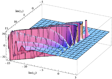
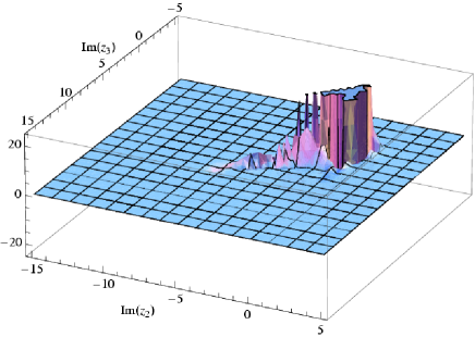
Figure 4: The real part of the integrand for the “sunset” diagram in eq. (51), for $p^{2}=\,$1, $m_{1}^{2}=\,$1, $m_{2}^{2}=\,$4, $m_{3}^{2}=\,$5. For the left panel, the integration contours have been chosen as straight lines parallel to the imaginary axis, and the $z_{1}$ integration has already been carried out. For the right panel, the contours have been deformed by a rotation in the complex plane, corresponding to $\theta=0.4$ in eq. (55).

However, for physical momenta, $p^{2}>0$, the integrand contains terms of the form

$$(-p^{2})^{z_{3}}=(p^{2})^{c_{3}+iy_{3}}(-1-i\epsilon)^{c_{3}+iy_{3}}=(p^{2})^{c_{3}+iy_{3}}e^{-i\pi c_{3}}e^{\pi y_{3}},$$ (53)

which grow exponentially for $y_{3}\to\infty$. While the contribution of the gamma functions is still dominant, so that the integral is formally finite, there is a long oscillating tail for positive values of $y_{3}$, see Fig. 4 (left). As a result, numerical integration routines often fail to converge in such a case.

This problem can be ameliorated by deforming the integration contours in the complex plane. To ensure that no pole of the integrand is crossed, all MB integrations need to be deformed in parallel. A possible choice is [67]

$$c_{i}+iy_{i}\to c_{i}+(\theta+i)y_{i}.$$ (54)

In eq. (53) this leads to

$$(-p^{2})^{z_{3}}=(p^{2})^{c_{3}+iy_{3}}e^{-i\pi(c_{3}+\theta y_{i})}e^{(\pi+\theta\log p^{2})y_{3}}.$$ (55)

By choosing $\theta$ appropriate, one can in principle cancel the exponentially growing term in (55), resulting in much improved numerical convergence, see Fig. 4 (right). The optimal value of $\theta$ for a given loop integral can be found by numerically probing the behavior of the integrand for large values $|y_{i}|$ of the integration variables.

A disadvantage of this method is that the parameter $\theta$ needs to be adjusted individually for each type of integral in a given loop calculation, and the choice depends on the values of the masses and external momenta. Moreover, there is no guarantee, in particular for non-planar diagrams, that a convergent result can always be obtained by varying the values of $\theta$. However, for certain classes of physical two-loop diagrams, this technique proved to be successful [67] and it was applied to the calculation of two-loop diagrams with triangle fermion subloops for the $Z\to b\bar{b}$ formfactor [69].

Further improvements of the numerical stability and convergence of the numerical MB integrals can be achieved through other variable transformations. For recent work in this direction, including possibilities for partial automatization, see $e.\,g.$ Refs. [70, 66].

2.4 Subtraction terms

In the previous two subsections, we discussed methods for the extraction of UV and IR divergences in terms of explicit powers in $1/\epsilon$, whose coefficients are finite multi-dimensional integrals that can be computed numerically. This subsection, on the other hand, will outline an alternative approach where the divergences are subtracted at the integrand level before any non-trivial integration is performed. The subtracted loop integrals are finite at every point in the integration region, and thus they are directly suitable for numerical evaluation. The subtraction terms are either simple enough so that they can be computed analytically and added back to the final expression, or they can be absorbed into renormalization counterterms that are then evaluated numerically.

Subtractions for multi-loop QED corrections:

In Ref. [71], a subtraction scheme has been presented that can be applied to theories with only Abelian gauge interactions, such as QED, and that works to arbitrary loop order. It has been used for the calculation of 3-loop [72, 73], 4-loop [74] and 5-loop [75] photonic corrections to the lepton anomalous magnetic moment.

For the construction of subtraction terms for the UV divergences, the technique of Kinoshita et al. starts with the Feynman parameter integral, see eq. (6), and proceeds as follows:

1. For a given subdiagram $\cal S$, its UV limit is taken by retaining the terms with the smallest number of external momenta in the numerator and taking the limit $x_{i}\sim{\cal O}(\delta)\to 0$ for all Feynman parameters $x_{i}$ associated with $\cal S$.

2. The function $\cal V$ in the Feynman parameter integral is replaced by $\cal V_{S}+V_{\bar{S}}$, where $\cal V_{S}$ is the $\cal V$ function of the subdiagram $\cal S$ and $V_{\bar{S}}$ is the corresponding function for the residual diagram that is obtained by shrinking $\cal S$ to a point.

3. In all other terms in the Feynman parameter integral, the UV limit from step 1 is taken, keeping only the leading terms in $\delta$.

4. It can be shown [71, 72] that the Feynman parameter integral then factorizes into two parts, one that contains the UV divergence of the subdiagram $\cal S$, and the other containing the contribution for the residual diagram $\cal\bar{S}$. The first factor can then be canceled against the UV-divergent part of the vertex or mass renormalization constant for $\cal S$.

Nested UV singularities are treated recursively from the minimal subdiagrams to larger subdiagrams, to the whole diagram, resulting in what is called a “forest” of subdiagrams [76].

Concerning the treatment of IR divergences, the situation for the computation of the lepton magnetic moment is somewhat special, since the magnetic form factor is free from any physical IR singularities, which would need to be canceled against soft real emission contributions. However, individual loop diagrams may still contain IR divergences, which cancel against the non-UV-divergent parts of the renormalization constants. In particular, IR divergences from self-energy subdiagrams cancel against the mass counterterm, while those from vertex subdiagrams cancel against the vertex counterterm [77].

To achieve this cancellation in practice, point-by-point in the Feynman parameter space, the IR-divergent parts of the renormalization constants need to be written in a form such that they can be combined with the Feynman parameter integral of the unrenormalized loop diagram. This can achieved by essentially inverting the factorization in step 4 above.

The IR subtraction terms may contain UV subdivergences, which must be removed as described above. Similarly, the IR divergences may appear within different subloops, leading to a nested structure. Therefore one needs to sum over all possibilities of recursively selecting IR-divergent subdiagrams [77] (again called “forests”).

These procedures can be cast into an algorithm and implemented in an automated computer program [77, 78], which can, in principle, tackle arbitrary high loop orders. However, the techniques have been tailored for QED corrections to magnetic moments of fermions, and they cannot be easily adapted to other problems.

Subtractions for general one- and two-loop processes:

For more general processes and interactions, it is more straightforward to apply singularity subtractions directly in loop momentum space, see eq. (1), rather than in Feynman parameter space. General subtraction schemes have been formulated for arbitrary one-loop amplitudes [79, 80, 81, 82, 83], but only partial extensions to the two-loop level are available [84, 83, 85, 86, 87].

Let us begin by reviewing the subtraction approach for one-loop integrals of the form

$$I^{(1)} =\int{\mathfrak{D}}q\;\frac{N(q)}{D_{1}\cdots D_{n}}, D_{j} =k_{j}^{2}-m_{j}^{2}=(q-p_{j})^{2}-m_{j}^{2},$$ (56)

where $N(q)$ is a polynomial in the loop momentum $q$, which may also depend on the external momenta and propagator masses. See Fig. 1 for a graphical representation.

A soft singularity occurs if a massless propagator $D_{i}$ is adjoined at both ends by two propagators $D_{i-1}$ and $D_{i+1}$ that become on-shell in the limit that the momentum of $D_{i}$ vanishes, while all other terms in the integrand remain regular in that limit. In other words, the necessary condition for a soft divergence is given by $m_{i}=0$ and $k_{i-1,i+1}\to 0$, $N(q)\not\to 0$ for $k_{i}\to 0$. It can be removed with the subtraction term [79, 80, 81, 82]

$${\cal G}_{\rm soft}^{(1)}=\frac{1}{D_{i-1}D_{i}D_{i+1}}\;\lim_{k_{i}\to 0}\biggl{[}N\prod_{\begin{subarray}{c}j\neq\\ i-1,\,i,\,i+1\end{subarray}}D^{-1}_{j}\biggr{]}.$$ (57)

This function can be easily integrated analytically in terms of the well known basic triangle function $C_{0}$. For explicit expressions, see $e.\,g.$ Refs. [80, 83].

A collinear singularity is encountered if two massless propagators meet at an external leg with vanishing invariant mass, $i.\,e.$ $m_{i}=m_{i-1}=0$ and $(k_{i}-k_{i-1})^{2}=(p_{i}-p_{i-1})^{2}=0$. It originates from the integration region where $k_{i-1}$ (and thus also $k_{i}$) becomes parallel to the external momentum $p_{i}-p_{i-1}$, $k_{i-1}=x(p_{i}-p_{i-1})$. At the same time, the numerator function should be regular in this limit, $N(q)\not\to 0$ for $q\to p_{i}$, which otherwise would be a fake singularity.

Collinear singularities associated with a soft singularity have already been removed by ${\cal G}_{\rm soft}^{(1)}$. For the remaining collinear singularities, the simplest subtraction term is given by [83]

$${\cal G}^{(1)}_{\rm coll} =\frac{1}{D_{i-1}D_{i}}\;\lim_{k_{i}\to p_{i}}\biggl{[}N\prod_{j\neq i-1,\,i}D^{-1}_{j}\biggr{]}.$$ (58)

In dimensional regularization, the integrated collinear subtraction term is simply zero. One drawback of this choice, however, is that ${\cal G}^{(1)}_{\rm coll}$ contains a UV divergence. This can be avoided by using the modified subtraction term [79, 82]

$${\cal G}^{(1)}_{\rm coll} =\frac{f_{\rm UV}(k_{i-1}^{2},k_{i}^{2})}{D_{i-1}D_{i}}\;\lim_{k_{i}\to p_{i}}\biggl{[}N\prod_{j\neq i-1,\,i}D^{-1}_{j}\biggr{]},$$ (59)

where $f_{\rm UV}$ vanishes for $k\to\infty$ but equals 1 in the collinear limit. A good choice is [82]

$$f_{\rm UV}(k_{i-1}^{2},k_{i}^{2}) =1-\frac{k_{i-1}^{2}k_{i}^{2}}{[(q-Q)^{2}-\mu_{\rm UV}^{2}]^{2}}.$$ (60)

Here $Q$ and $\mu_{\rm UV}$ are a constant four-vector and constant mass parameter, respectively, which can be chosen to be complex to prevent the appearance of additional singularities from ${\cal G}^{(1)}_{\rm coll}$ inside the integration region. An analytical result for the integrated collinear subtraction term can be found in Ref. [82].

At this point, the loop amplitude reads

$$I^{(1)} =\int{\mathfrak{D}}q\;\biggl{[}\frac{N(q)}{D_{1}\cdots D_{n}}-\sum_{\rm soft}{\cal G}_{\rm soft}^{(1)}-\sum_{\rm coll.}{\cal G}_{\rm coll}^{(1)}\biggr{]}+\sum_{\rm soft}G_{\rm soft}^{(1)}+\sum_{\rm coll.}G_{\rm coll}^{(1)},$$ (61)

where the sums run over all soft and collinear singularities in $I^{(1)}$, and $G_{x}^{(1)}=\int{\mathfrak{D}}q\,{\cal G}^{(1)}_{x}$ are the integrated subtraction terms. The first term in (61) is free of IR divergences, but may still contain UV divergences. These may be extracted with the help of Feynman parameters [83] or by introducing suitable UV subtraction terms [79, 82].

In order to do so, it is helpful to first write the integrand in (61) on a common denominator,

$$\frac{\widetilde{N}(q)}{D_{1}\cdots D_{n}}\equiv\frac{N(q)}{D_{1}\cdots D_{n}}-\sum_{\rm soft}{\cal G}_{\rm soft}^{(1)}-\sum_{\rm coll.}{\cal G}_{\rm coll}^{(1)},$$ (62)

where $\widetilde{N}(q)$ is a polynomial in $q$ and a rational function in the other parameters. Then a UV subtraction term for vertices and fermion self-energies can be constructed as [79]

$${\cal G}_{\rm UV}^{(1)} =\frac{\widetilde{N}_{\rm UV}(q)}{(q^{2}-\mu^{2}_{\rm UV})^{n}}+{\cal G}_{\rm UV,fin}^{(1)},$$ (63)

where $\widetilde{N}_{\rm UV}$ contains only terms of order $q^{2n-4}$ or higher from $\widetilde{N}(q)$. It is always possible to add a UV-finite piece, ${\cal G}_{\rm UV,fin}^{(1)}$, to the UV subtraction term, which can be adjusted according to some renormalization scheme, such as the $\overline{\text{MS}}$ scheme [79, 82].

Figure 5: UV-divergent one-loop self-energy diagrams.

For instance, the UV subtraction term for a gauge-interaction correction to a fermion self-energy, see Fig. 5 (a), is given by

$$\Sigma_{\rm UV}^{f(1)} =\frac{g^{2}}{16\pi^{2}}\,\frac{\gamma^{\mu}(\makebox[0.34444pt][l]{$q$}/+\frac{1}{2}\makebox[0.86108pt][l]{$p$}/+m_{f})\gamma_{\mu}}{[q^{2}-\mu^{2}_{\rm UV}]^{2}}+\Sigma_{\rm UV,fin}^{f(1)}.$$ (64)

For boson self-energies, the form (63) is not adequate due to the presence of quadratic divergences in the loop integral. Instead one needs to perform an expansion of the loop propagators in addition to the numerator $\widetilde{N}$. For example, one can construct in this way the following subtraction terms for the scalar self-energy as in Fig. 5 (b):

$$\Sigma_{\rm UV}^{\phi(1)} =-\frac{g^{2}}{4\pi^{2}}\,\biggl{[}\frac{1}{q^{2}-\mu^{2}_{\rm UV}}+\frac{p^{2}+q\cdot p+\mu_{\rm UV}^{2}-3m^{2}}{[q^{2}-\mu^{2}_{\rm UV}]^{2}}-\frac{2(q\cdot p)^{2}}{[q^{2}-\mu^{2}_{\rm UV}]^{3}}\biggr{]}+\Sigma_{\rm UV,fin}^{\phi(1)}.$$ (65)

Expressions for other UV subtraction terms can be found in Ref. [79] and, including the finite part required for $\overline{\text{MS}}$ renormalization, in Ref. [82].

Note that there is some ambiguity from the possibility of shifting $q$ by a fixed amount in (63), which can be exploited to make the UV subtraction term better behaved for numerical evaluation.

At the two-loop level, the situation becomes more involved. As long as a UV or IR singularity is associated with one of the two subloops only, essentially the same subtraction terms as above can be used [83, 87]. The only difference is that the analytically integrated subtraction terms need to be evaluated up to ${\cal O}(\epsilon)$.

In addition, subtraction terms for global UV divergences of both subloops have been defined [83, 85, 86]. They are given in terms of simple two-loop vacuum and self-energy integrals, which are known analytically [26, 88, 89]. However, no subtraction terms for overlapping IR divergences between the two subloops have been constructed to date.

Contour deformation:

After all IR and UV singularities have been subtracted, the loop integral is ensured to have a finite result. However, the integrand may still contain singularities associated with thresholds of the corresponding loop diagram, which lead to problems for the numerical integration. This situation is similar to what has been discussed in section 2.2. One approach to circumvent these singularities, therefore, is to introduce Feynman parameters, carry out the loop momentum integration, and then apply the complex contour deformation in eq. (40). This method is implemented in the public computer code Nicodemos [83].

In some situations, it may be advantageous not to perform the loop momentum integration analytically, but to evaluate the loop momentum and Feynman parameter integrals together in a multi-dimensional loop integration [57, 82]. This offers more flexibility in choosing a contour deformation that keeps the integrand fairly smooth everywhere and avoids large cancellations between different integration regions.

Alternatively, the numerical integration, with a suitable complex contour deformation, may be carried out directly in the $q$ momentum space [90, 91, 92, 93, 94]. This has the advantage of keeping the integration dimensionality low for multi-leg amplitudes, as well as to avoid a denominator raised to a high power, which can cause numerical convergence problems. It may also be beneficial for combining the virtual loop corrections with contributions from real emission of extra partons [90, 91, 95, 96]. On the other hand, the choice of the contour is more complicated for the $q$-momentum integral.

In the following, the contour deformation for the case of massless loop propagators will be sketched. A detailed description can be found in Ref. [92]. The integrand has singularities for $(q-p_{j})^{2}=0$. The goal is to avoid the singularities by shifting the loop momentum into the complex plane in their vicinity,

$$q^{\mu}\to q^{\prime\mu}=q^{\mu}+i\lambda\kappa^{\mu}_{0}(q),$$ (66)

where $\lambda$ is a small parameter. Then

$$(q^{\prime}-p_{j})^{2}=(q-p_{j})^{2}+2i\lambda\,(q-p_{j})\cdot\kappa_{0}(q)+{\cal O}(\lambda^{2}).$$ (67)

To stay compatible with the Feynman $i\varepsilon$ prescription, one must demand $(q-p_{j})\cdot\kappa_{0}(q)\geq 0$. This condition can be interpreted geometrically as the requirement that $\kappa_{0}$ point to the interior (for the $>$ sign) or along the boundary (for the $=$ sign) of a light cone from the point $p_{j}$.

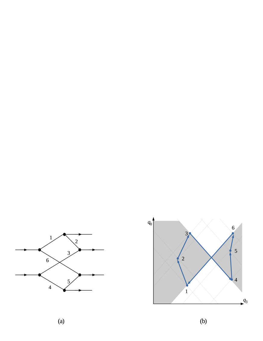
Figure 6: A sample $2\to 4$ diagram topology (a); and the projection of its kinematics onto the $q_{0}$–$q_{3}$ plane (b).

To see how this can be achieved in practice, it is illustrative to consider a concrete example, such as the diagram topology for a $2\to 4$ process shown in Fig. 6 (a). Figure 6 (b) shows the projection of the four-dimensional $q$-space onto the $q_{0}$–$q_{3}$ plane for a sample kinematical configuration. Each dot corresponds to a possible point $q=p_{j}$, while an upward/downward line represents an outgoing/incoming external momentum. The dashed lines indicate the light cones from the points $p_{j}$.

Now let us consider the deformation

$$\kappa_{0} =-\sum_{j}c_{j}(q-p_{j}),$$ (68)

where $c_{j}(q)\geq 0$ is a function to be specified below. For all $p_{i}$ lying inside the backward light cone from $p_{j}$, one has $(q-p_{j})\cdot(q-p_{i})=(q-p_{j})^{2}+(q-p_{j})\cdot(p_{j}-p_{i})>0$ when $q$ is on the surface of the backward light cone ($i.\,e.$ when $(q-p_{j})^{2}=0$ and $q_{0}-p_{j,0}<0$). Therefore, $c_{i}>0$ is a good choice in these cases to ensure that $(q-p_{j})\cdot\kappa_{0}(q)\geq 0$. On the other hand, when $q$ is on the forward light cone, one has $(q-p_{j})\cdot(q-p_{i})<0$ and thus we choose $c_{i}=0$.

Similarly, for all $p_{i}$ lying inside the forward light cone from $p_{j}$, one has $(q-p_{j})\cdot(q-p_{i})>0$ ($<0$) when $q$ is on the surface of the forward (backward) light cone, and thus we choose $c_{i}>0$ ($c_{i}=0$) in these cases. This can be realized through

$$c_{j}=h_{+}(q-p_{j+1})\,h_{-}(q+p_{j+1})\,g(q),$$ (69)

where $h_{\pm}(k)$ are smooth functions with the properties $h_{\pm}(k)=0$ for $|\vec{k}|>\pm k_{0}$ and $h_{\pm}(k)\to 1$ for $k_{0}\mp|\vec{k}|\to\infty$. $g(k)$ is a smooth function that vanishes for $k^{\mu}\to\infty$, to ensure that the contour deformation goes to zero at the integral boundaries. The precise definition of $h_{\pm}$ and $g$ can be found in Ref. [92].

The choice (69) ensures that $(q-p_{j})\cdot\kappa_{0}(q)\geq 0$ if $q$, $p_{j}$ and the $p_{i}$ are restricted to lie either inside the left or inside the right shaded regions of Fig. 6 (b). While some of the terms in (68) are zero due to the $h_{\pm}$ functions, there is always at least one non-zero term with the correct sign. The only exceptions are the points $q-p_{j}=0$ and the lines $q=xp_{j}-(1-x)p_{i}$ for $0<x<1$ and $(p_{j}-p_{i})^{2}-0$. In these two cases, which correspond to soft and collinear singularities, $(q-p_{j})\cdot\kappa_{0}(q)=0$, $i.\,e.$ the contour is pinched. However, the soft and collinear singularities have been subtracted already, so these points do not require any special contour deformation.

The treatment of the unshaded regions in Fig. 6 (b) requires the consideration of special cases for the coefficients $c_{j}$ and the introduction of additional terms in eq. (68). See Ref. [79] for more information.

Finally, one has to define the scaling parameter $\lambda$ in (67). To improve the smoothness of the integrand and increase the speed of convergence, it is advantageous to pick as large a value of $\lambda$ as possible. On the other hand, one must ensure that no other singularities are crossed by the contour as $\lambda$ is increased. To balance these two requirements, it is advantageous to define $\lambda$ as a function of $q$. Suitable choices that avoid singularities from other propagators and from the UV subtraction terms are given in Ref. [79] and Ref. [97], respectively.

While this algorithm for the $q$-space contour deformation is rather involved, it is straightforward to implement as a numerical computer program. Extensions to handle massive loop propagators [93] and multi-loop integrals [94] are also known. Techniques to improve the efficiency of the numerical integration are discussed in Refs. [98, 97]. One notable application of the direct contour deformation methods is the calculation of one-loop QCD corrections to five-, six- and seven-jet production in $e^{+}e^{-}$ annihilation [99].

Related methods:

Instead of carrying out all $4L$ dimensions of the loop integral numerically, where $L$ is the number of loops, one can also try to evaluate as many of the integrations analytically as possible, to arrive at a low-dimensional numerical integral. This approach has been pioneered for two-loop integrals in Ref. [100]. For this purpose, the loop momenta $q_{1}$ and $q_{2}$ are split into their energy components, $q_{10}$ and $q_{20}$, and their momentum components parallel and transverse to an external momentum, $q_{1||}$, $q_{1\perp}$, $q_{2||}$, and $q_{2\perp}$.

For a general finite two-loop self-energy integral, it was shown that the momentum-component integrations can be performed analytically, resulting in a two-dimensional integral representation related to the $q_{10}$ and $q_{20}$ integrations [100, 101]. The finiteness of the integral is assumed to have been achieved through suitable subtractions. This method can be straightforwardly extended to general $q_{1,2}$-dependent tensor structures in the numerator of the integral, by splitting these into components in the same fashion [85, 86].

Similarly, two-dimensional integral representations were obtained for two-loop vertex-type master integrals, which have a trivial numerator function $N(q_{1},q_{2})\equiv 1$ [101, 102]. Three-dimensional integral representations for certain two-loop box master integrals were obtained in Ref. [103]. These techniques have been applied towards the calculation of dominant two-loop corrections to Higgs-boson decays in the limit of a large Higgs mass [104].

An attractive feature of this method is the low dimension of the resulting numerical integrals, which thus can be evaluated with deterministic integration algorithms to high precision. However, it has certain shortcomings: No general procedure for numerator terms in three- and higher-point two-loop integrals is known. In addition, loop diagrams with internal threshold have singularities in the interior of the integration region where the integrand denominator vanishes. In Refs. [86, 105], these singular points are circumvented by assigning a non-zero numerical value to the $\varepsilon$ parameter of the Feynman $i\varepsilon$ prescription. While in principle this renders the integrand finite everywhere in the integration region, the numerical integration will converge relatively slowly near such a point.

2.5 Dispersion relations

Dispersion relations are based on analytical properties of field theory amplitudes, and they can be used to construct the value of a loop diagram from its imaginary part. The latter is related to the discontinuity across the branch cuts between different Riemann sheets. It can be constructed from cuts through internal lines of the loop diagram using the Cutkosky rules [106]. See Ref. [107] for a pedagogical introduction.

Generically, a dispersion relation has the form

$$I(q^{2}) =\frac{1}{2\pi i}\int_{s_{0}}^{\infty}\frac{\Delta I(s)}{s-q^{2}-i\varepsilon},$$ (70)

where $q^{2}$ is a characteristic squared external momentum, and $\Delta I(s)=\frac{1}{2i}\,{\rm Im}\,I(s)$ is the discontinuity of the loop integral $I(s)$. The idea is that the imaginary part is relatively simple to determine from the Cutkosky rules, and then one can use eq. (70) to find the result for the whole function $I(s)$. Note that the dispersion integral can be applied to a multi-loop diagram itself or to some subloop, and either choice may be more convenient for different types of Feynman diagrams. If possible, one may try to perform the $s$-integral in (70) analytically, see Ref. [108] for early applications. Here, we want to focus on the numerical evaluation of the dispersion integral.

Figure 7: One-loop scalar self-energy diagram with the cut contributing to its discontinuity (a); and a general two-loop scalar diagram with a self-energy subloop (b).

The simplest case is the one-loop scalar self-energy function, see Fig. 7 (a), which will be called $B_{0}(p^{2},m_{1}^{2},m_{2}^{2})$ in the following. As a function of $p^{2}$, it exhibits a discontinuity along the positive real axis for $p^{2}>(m_{1}+m_{2})^{2}$. The discontinuity can be calculated by cutting the diagram through the $m_{1}$ and $m_{2}$ lines, resulting in a $1\to 2$ decay process. The result in dimensional regularization is

$$B_{0}(p^{2},m_{1}^{2},m_{2}^{2}) =\int_{(m_{1}+m_{2})^{2}}^{\infty}{\rm d}s\,\frac{\Delta B_{0}(s,m_{1}^{2},m_{2}^{2})}{s-p^{2}-i\varepsilon},$$ (71)

$$\Delta B_{0}(s,m_{1}^{2},m_{2}^{2}) =\frac{\Gamma(D/2-1)}{\Gamma(D-2)}\,\frac{\lambda^{(D-3)/2}(s,m_{1}^{2},m_{2}^{2})}{s^{D/2-1}},$$ (72)

where $\lambda(a,b,c)$ is defined in (24). With this expression, a scalar two-loop integral with a self-energy subloop, see Fig. 7 (b), can be written as [109]

$$I^{(2)}_{\rm fig\ref{fig:dispse}b}(\{p_{i}\};\{m_{i}^{2}\})=- \int_{(m_{N}+m_{N+1})^{2}}^{\infty}{\rm d}s\;\Delta B_{0}(s,m_{N}^{2},m_{N+1}^{2})$$ (73)

$$\times \int{\mathfrak{D}}q\,\frac{1}{q^{2}-s}\,\frac{1}{(q+p_{1})^{2}-m_{1}^{2}}\cdots\frac{1}{(q+p_{N-1})^{2}-m_{N-1}^{2}}.$$

The integral in the second line is a $N$-point one-loop function, for which the well-known analytical expression [110, 111] can be inserted. The remaining integration over $s$ can then be carried out numerically.

This approach can be easily extended to deal with two-loop integrals with a self-energy subloop and a non-trivial tensor structure ($i.\,e.$ with non-trivial terms in the numerator of the integrand). For this purpose, one first decomposes the self-energy subloop into a sum of Lorentz covariant building blocks [4, 112]. For example, a vector-boson and a fermion self-energy can be written as

$$\Sigma_{\mu\nu}^{V}(q) =\Bigl{(}g_{\mu\nu}-\frac{q_{\mu}q_{\nu}}{q^{2}}\Bigr{)}\Sigma_{\rm T}^{V}(q^{2})+\frac{q_{\mu}q_{\nu}}{q^{2}}\Sigma_{\rm L}^{V}(q^{2}),$$ (74)

$$\Sigma^{f}(q) =\makebox[0.34444pt][l]{$q$}/P_{\rm L}\Sigma^{f}_{\rm L}(q^{2})+\makebox[0.34444pt][l]{$q$}/P_{\rm R}\Sigma^{f}_{\rm R}(q^{2})+m_{f}\Sigma^{f}_{\rm S}(q^{2}),$$ (75)

respectively. Here $P_{\rm L,R}=\frac{1}{2}(1\mp\gamma_{5})$. Inserting these expressions into the second loop, one obtains a dispersion integral similar to (73), except that the $q$-integral is in general a one-loop tensor integral. The latter can be evaluated analytically with the standard Passarino-Veltman decomposition [3, 111, 113].

Figure 8: Cuts through the basic scalar two-loop self-energy diagram with triangle subloops.

In addition, the dispersion approach has been used to derive a one-dimensional integral representation for the scalar self-energy integral in Fig. 8 [114]. The discontinuity of this diagram has been obtained by summing over the contributions from all cuts shown in the figure, see Ref. [114] for more details. The reduction of tensor integrals with the topology in Fig. 8 is described in Ref. [4].

For the two-loop examples discussed in this section so far, the dispersion relation method leads to one-dimensional integral expressions, which can be evaluated to a very high precision with a deterministic integration algorithm. The numerical integrals are free from problematic singularities in the interior of the integration interval, even for loop diagrams with physical thresholds. In some cases, the integrand may contain terms proportional to $1/(s-p^{2}-i\varepsilon)$, which can be rendered smooth with the simple variable transformation $s\to t=\log(s-p^{2}-i\varepsilon)$.

On the other hand, the method also has several drawbacks. Firstly, there is no automated treatment of UV and IR divergences. These manifest themselves as singularities at the lower or upper limit of the dispersion integral, respectively, and they must be removed from the dispersion integral using suitable subtraction terms. These terms have to be derived by hand for each different class of diagram.

For instance, a two-loop diagram of the form in Fig. 7 (b) has a UV divergence stemming from the self-energy subloop, but no global UV divergence if it has at least five propagators. The subloop UV divergence can be removed by subtracting the term

$$B_{0}(M^{2},m_{N}^{2},m_{N+1}^{2})\int{\mathfrak{D}}q\,\frac{1}{(q+p_{1})^{2}-m_{1}^{2}}\cdots\frac{1}{(q+p_{N-1})^{2}-m_{N-1}^{2}},$$ (76)

which is a product of two one-loop functions. Here $M^{2}$ is an arbitrary mass parameter. The subtracted dispersion integral then reads

$$I^{(2)}_{\rm fig\ref{fig:dispse}b,sub}(\{p_{i}\};\{m_{i}^{2}\})=- \int_{(m_{N}+m_{N+1})^{2}}^{\infty}{\rm d}s\;\frac{\Delta B_{0}(s,m_{N}^{2},m_{N+1}^{2})}{s-M^{2}}$$ (77)

$$\times \int{\mathfrak{D}}q\,\frac{q^{2}-M^{2}}{[q^{2}-s][(q+p_{1})^{2}-m_{1}^{2}]\cdots[(q+p_{N-1})^{2}-m_{N-1}^{2}]}.$$

The integrand behaves like $s^{-2-\epsilon}$ for $s\to\infty$ and thus the integral is UV-finite. Additional subtraction terms are needed for IR singularities.

Figure 9: Reduction of triangle subloop to self-energy subloop by means of a Feynman parameter.

Secondly, another limitation of the dispersion methods is the difficulty of extending the elegant examples mentioned above to more complicated two-loop topologies. One possibility is the introduction of Feynman parameters to reduce triangle subloops to self-energy subloops, which then can be evaluated as in (73) [115]. For example, the propagators 1 and 2 of the two-loop diagram in Fig. 9 can be combined using a Feynman parameter $x$, resulting in a diagram with a self-energy subloop, where one propagator is raised to the power two and has an $x$-dependent mass and $x$-dependent external momenta:

$$\begin{gathered}\ [(q+p_{1})^{2}-m_{1}^{2}]^{-1}\;[q^{2}-m_{2}^{2}]^{-1}=\int_{0}^{1}{\rm d}x\;[(q+xp_{1})^{2}-m_{\overline{12}}^{2}]^{-2}\\ m_{\overline{12}}^{2}=x\,m_{1}^{2}+(1-x)m_{2}^{2}-x(1-x)p_{1}^{2}.\end{gathered}$$ (78)

The integration over Feynman parameters, as well as the dispersion integral, are performed numerically. In this way, all basic two-loop vertex topologies can be represented by at most two-dimensional numerical integrals.

However, the dispersion relation is only defined for non-negative masses $m_{1,2}\geq 0$, whereas the Feynman-parameter dependent mass $m_{\overline{12}}$ can in general also become negative. Thus, the combination of dispersion relations and Feynman parameters can only be applied to restricted parameter regions.

Dispersion relations have been used for the calculation of two-loop corrections to the prediction of the $W$-boson mass from muon decay in the full Standard Model [116, 117], for subsets of two-loop diagrams contributing to the $Z\to f\bar{f}$ formfactors [118, 112, 115], as well as for two-loop quark loop corrections to Bhabha scattering [119].

2.6 Bernstein-Tkachov method

The Bernstein-Tkachov method [120, 121] uses analytic properties of the integrand to render singularity peaks into a smoother form that is suitable for numerical integration without complex contour deformation.

It can be applied most straightforwardly for one-loop integrals, see eq. (42), whose Feynman parametrization can be written as

$$I^{(1)} =(-1)\Gamma(n-D/2)\int_{0}^{1}dx_{1}\cdots dx_{n}\;\delta\Bigl{(}1-\sum_{i=1}^{n}x_{i}\Bigr{)}\;{\cal Q}(\vec{x}_{e})\,{\cal V}^{-n+D/2}(\vec{x}_{e}),$$ (79)

where $\cal Q$ and $\cal V$ are polynomials in $\vec{x}_{e}\equiv(x_{1},\dots,x_{n})^{\top}$, which also depend on the internal masses and external momenta. A non-trivial function $Q\neq 1$ occurs as a result of a non-trivial numerator function $N(q)$ in (42). The $x_{n}$-integral can be evaluated to eliminate the $\delta$-function, yielding

$$I^{(1)} =(-1)\Gamma(n-D/2)\int_{0}^{1}dx_{1}\int_{0}^{1-x_{1}}dx_{2}\cdots\int_{0}^{1-\sum_{i=1}^{n-2}x_{i}}dx_{n-1}\;{\cal Q}(\vec{x})\,{\cal V}^{-\nu-\epsilon}(\vec{x}),$$ (80)

where $\vec{x}\equiv(x_{1},\dots,x_{n-1})^{\top}$, $\nu=n-2$ and $\epsilon=(4-D)/2$. $\cal V$ is a quadratic form in the Feynman parameters,

$${\cal V}(\vec{x}) =\vec{x}^{\top}H\vec{x}+2\vec{K}^{\top}\vec{x}+L,$$ (81)

where $H$ is a $(n{-}1){\times}(n{-}1)$-matrix, $\vec{K}$ is a $(n{-}1)$-dimensional vector, and $L$ is a scalar in Feynman-parameter space. For $\nu>0$, the integrand in (80) exhibits singular behavior when ${\cal V}(\vec{x})$ becomes zero. This can occur for points $\vec{x}$ inside the integration region if the loop diagram has internal thresholds.

It was shown by Tkachov [121] that the following relation holds:

$${\cal V}^{-\nu-\epsilon}=\frac{1}{B}\biggl{[}1-\frac{(\vec{x}+\vec{A})^{\top}\vec{\partial}_{x}}{2(1-\nu-\epsilon)}\biggr{]}{\cal V}^{-\nu-\epsilon+1},$$ (82)

where

$$B =L-\vec{K}^{\top}H^{-1}\vec{K}, \vec{A} =H^{-1}\vec{K}, \vec{\partial}_{x} =\bigl{(}\tfrac{\partial}{\partial x_{1}},\dots,\tfrac{\partial}{\partial x_{n-1}}\bigr{)}^{\top}.$$ (83)

This relation can be used to increase the power of the polynomial ${\cal V}(\vec{x})$. For example, for the class of one-loop three-point functions with two independent Feynman parameters, one finds

$$\int_{0}^{1}dx_{1}\int_{0}^{1-x_{1}}dx_{2}\;{\cal Q}(\vec{x})\,{\cal V}^{-\nu-\epsilon}(\vec{x})$$

$$=\frac{1}{2(1-\nu-\epsilon)B}\,\biggl{\{}\int_{0}^{1}dx_{1}\int_{0}^{1-x_{1}}dx_{2}\;\biggl{[}(2-\nu-\epsilon){\cal Q}(\vec{x})+\sum_{i=1}^{2}A_{k}\frac{\partial\cal Q}{\partial x_{k}}\biggr{]}{\cal V}^{-\nu-\epsilon+1}(\vec{x})$$

$$\qquad\qquad\qquad\qquad+\int_{0}^{1}dx_{1}\;A_{2}{\cal Q}(\vec{x})\,{\cal V}^{-\nu-\epsilon+1}(\vec{x})\Big{|}_{x_{2}=0}+\int_{0}^{1}dx_{2}\;A_{1}{\cal Q}(\vec{x})\,{\cal V}^{-\nu-\epsilon+1}(\vec{x})\Big{|}_{x_{1}=0}$$

$$\qquad\qquad\qquad\qquad-\int_{0}^{1}dx_{1}\;(1+A_{1}+A_{2}){\cal Q}(\vec{x})\,{\cal V}^{-\nu-\epsilon+1}(\vec{x})\Big{|}_{x_{2}=1-x_{1}}\biggr{\}}.$$ (84)

Here the one-dimensional integrals stem from performing an integration-by-parts operation on the derivative term in eq. (82). This operation can be performed repeatedly until the power of $\cal V$ is reduced to ${\cal V}^{-\epsilon}$. Then one can simply perform a Laurent expansion about $\epsilon=0$ to extract the UV divergent contributions, while the finite terms contain only logarithms of $\cal V$ as the worst singularities. These can be integrated efficiently with standard numerical algorithms.

IR divergent configurations can be either evaluated by suitable rearrangements of the Feynman parameter integral such that one Feynman parameter integration can be performed analytically [122]. With a subsequent Laurent expansion about $\epsilon=0$, the IR divergent terms are obtained explicitly. Alternatively, the IR divergent cases can be handled with the help of sector decomposition or Mellin-Barnes representations [123]. See sections 2.2 and 2.3 for the definition of these methods.

For two-loop integrals, the Bernstein-Tkachov relation (82) cannot be employed straightforwardly, since in general the polynomial $\cal V$ in (7) is not a quadratic form in the Feynman parameters. Instead, one may apply eq. (82) to the one-loop subdiagram with the largest number of internal lines [122]. In other words, one introduces two sets of Feynman parameters, one set $\vec{x}$ for the subloop with most propagators, and another set $\vec{y}$ for the remainder of the two-loop diagram. The Bernstein-Tkachov relation (82) is then applied to the variables $\vec{x}$, but now the coefficients $A_{ij}$, $P_{i}$ and $M$ are dependent on $\vec{y}$. Repeated application of (82) can then be used to raise the power of the denominator function ${\cal V}(\vec{x},\vec{y})$. Additional variable transformations can be used to ensure that one encounters at most logarithmic behavior of the integrand near singularities in the interior of the integration region [124, 125]. Furthermore, oftentimes some of the Feynman parameter integrations can be carried out analytically, thus reducing the dimensionality of the numerical integral [125].

Integrals with non-trivial tensor structures in the numerator can be handled with essentially the same approach, since the contribution of the numerator terms can be absorbed into the function $\cal Q$ in eq. (79). See Ref. [126] for more details.

UV and IR divergences occurring in one subloop of a two-loop diagram can be extracted by performing the Feynman parameter integrations associated with this subloop analytically and then expanding the result in powers of $\epsilon$ [127]. Sector decomposition can be used to simplify this procedure in more complicated cases. This approach leads to compact results that can be efficiently integrated numerically, but it requires a separate derivation for each different loop topology. Alternatively, the singularities can also be removed with suitable subtraction terms before the Bernstein-Tkachov relation is applied [112]. The subtraction methods are described in section 2.4 in more detail.

One difficulty of the original Bernstein-Tkachov formula (82) is the appearance of the factor $B$ in the denominator. It may vanish for certain configurations, some of which correspond to physical singularities. However, one can also find $B\sim 0$ even in cases where the loop integral is regular. In this situation, different terms in the numerator of (82) cancel each other, leading to potential numerical instabilities. For a subloop within a two-loop diagram, $B$ depends on the Feynman parameters $\vec{y}$ of the outer loop, and thus one can encounter $B\sim 0$ for particular values of $\vec{y}$ inside the integration region, again resulting in numerical instabilities.

Therefore, it is necessary to have a special treatment for regular integrals with $B\sim 0$. For instance, a Taylor expansion about $B=0$ leads to a well-defined and numerically stable expression [123, 125]. In Ref. [128], a modified Bernstein-Tkachov-like relation was proposed that avoids the appearance of the $1/B$ factors altogether. Writing

$${\cal V}(\vec{x}) =Q(\vec{x})+B, Q(\vec{x}) =(\vec{x}+\vec{A})^{\top}H\;(\vec{x}+\vec{A}),$$ (85)

it can be shown that the following relation holds [128]:

$${\cal V}(\vec{x})^{-\nu-\epsilon} =\bigl{[}\beta+(\vec{x}+\vec{A})^{\top}\vec{\partial}_{x}\bigr{]}\int_{0}^{1}dy\,y^{\beta-1}[Q(\vec{x})y+B]^{-\nu-\epsilon},$$ (86)

where $\beta>0$ is an arbitrary constant. The integral over $y$ can be evaluated analytically in terms of the hypergeometric function ${}_{2}F_{1}$. The $\vec{\partial}_{x}$ can be eliminated by performed integration by parts in the $\vec{x}$-integral. Expanding the latter around $\epsilon=0$ then leads to an expression with a lower power of $Q(\vec{x})+B$ than on the left-hand side of eq. (86). This procedure can be applied iteratively with suitable values of $\beta$ until sufficiently smooth integrals are obtained.

The advantage of the Bernstein-Tkachov method and related techniques is the fact that it leads to relatively simple and smooth numerical integrals that converge quickly and reliably. For most two-loop configurations with up to three external legs, one can derive numerical integrals with just two or three dimensions. UV and IR divergent configurations can also be handled. However, each different diagram topology and IR singularity configuration requires a different derivation of the final integral representation, so that this step cannot be automatized easily.

Applications of the Bernstein-Tkachov method include two-loop electroweak corrections to $Z\to f\bar{f}$ formfactors [112, 129, 130] and next-to-leading order electroweak corrections to the Higgs-boson couplings to photons and gluons [131].

2.7 Differential equations

Differential equations [29] are a well-known tool for the analytical evaluation of loop integrals. However, they may also be integrated numerically. For concreteness, let us begin by illustrating this approach for the example for two-loop self-energy integrals, based on the work in Refs. [132, 133, 134].

Figure 10: A convenient basis of two-loop self-energy master integrals. All propagators are assumed to be scalars.

Using integration by parts or other reduction methods, an arbitrary two-loop self-energy integral can be written as a linear combination of five two-loop master integrals shown in Fig. 10 and terms involving one-loop integrals. The vacuum integral $T_{0}$ is known analytically in terms of dilogarithms [26, 88, 89]. The remaining integrals $I_{k}(p^{2};\{m_{n}^{2}\})$ depend on the external invariant momentum, $p^{2}$. The derivative of $I_{k}$ with respect to $p^{2}$ can be computed at the integrand level by using

$$\frac{\partial}{\partial(p^{2})}I_{k} =\frac{1}{2p^{2}}\,p^{\mu}\frac{\partial}{\partial(p^{\mu})}I_{k}.$$ (87)

From the expression on the right-hand side of (87) one obtains self-energy integrals with additional propagators and/or numerator terms. These again can be reduced to a linear combination of the $I_{k}$, $T_{0}$ and one-loop integrals. Thus one arrives at a differential equation of the form

$$\frac{\partial}{\partial(p^{2})}I_{k} =\sum_{l}f_{kl}\,I_{l}+g_{k}.$$ (88)

The coefficients $f_{kl}$ are rational functions of the masses $m_{n}$, the momentum invariant $p^{2}$ and the dimension $D$. The inhomogeneous part involves the two-loop vacuum function $T_{0}$ as well as one-loop functions, all of which are known analytically.

To eliminate the dependence of the space-time dimension $D=4-2\epsilon$, all terms in (88) can be expanded in powers of $\epsilon$. In the absence of IR divergences, the master integrals $I_{k}$ may contain UV $1/\epsilon$ and $1/\epsilon^{2}$ poles, so that one can write

$$I_{k} =I_{k}^{[-2]}\,\epsilon^{-2}+I_{k}^{[-1]}\,\epsilon^{-1}+I_{k}^{[0]}+{\cal O}(\epsilon),$$

$$f_{kl} =f^{[0]}_{kl}+f^{[1]}_{kl}\,\epsilon+f^{[2]}_{kl}\,\epsilon^{2}+{\cal O}(\epsilon^{3}),$$ (89)

$$g_{k} =g_{k}^{[-2]}\,\epsilon^{-2}+g_{k}^{[-1]}\,\epsilon^{-1}+g_{k}^{[0]}+{\cal O}(\epsilon).$$

For general situations, the coefficient functions $f_{kl}$ may have singular terms in $\epsilon$, so that the integrals $I_{k}$ need to be expanded to higher powers $\epsilon$ beyond $\epsilon^{0}$. However, for the class of two-loop self-energy integrals this is not needed. Inserting (89) into (88) one obtains

$$\frac{\partial}{\partial(p^{2})}I_{k}^{[-2]} =\sum_{l}f_{kl}^{[0]}\,I_{l}^{[-2]}+g_{k}^{[-2]},$$ (90)

$$\frac{\partial}{\partial(p^{2})}I_{k}^{[-1]} =\sum_{l}\bigl{(}f_{kl}^{[0]}\,I_{l}^{[-1]}+f_{kl}^{[1]}\,I_{l}^{[-2]}\bigr{)}g_{k}^{[-1]},$$ (91)

$$\frac{\partial}{\partial(p^{2})}I_{k}^{[0]} =\sum_{l}\bigl{(}f_{kl}^{[0]}\,I_{l}^{[0]}+f_{kl}^{[1]}\,I_{l}^{[-1]}+f_{kl}^{[2]}\,I_{l}^{[-2]}\bigr{)}g_{k}^{[0]}.$$ (92)

The differential equations (90) and (91) are simple enough such that they can be solved analytically [132, 133]. On the other hand, the system (92) of first-order linear differential equations can be integrated numerically from an initial value $p_{0}^{2}$, for example using the Runge-Kutta algorithm. A simple choice for the boundary value is $p_{0}^{2}=0$, where all integrals $I_{k}(p_{0}^{2})$ reduce to vacuum integrals and thus can be evaluated analytically.

Similar to other methods discussed in the previous subsections, difficulties can arise from singular points of the integrand associated with thresholds. While these singularities are formally integrable by virtue of the Feynman $i\varepsilon$ prescription, they can lead to numerical instabilities and convergence problems. This problem can be avoided by using a complex integration contour. A practical complex contour was suggested in Ref. [133]: $0\to i\delta\to p^{2}+i\delta\to p^{2}$, $i.\,e.$ the integration initially moves along the imaginary axis to a fixed value $\delta>0$, then parallel to the real axis, and finally back to the real axis.

Special cases occur if the integration endpoint $p^{2}$ is itself near a threshold. In this case, one could use this threshold as the initial value $p_{0}^{2}$ for the numerical integration, which requires the analytical evaluation of the integrals at the threshold value to obtain the boundary value [133, 135]. In this context, it is worth mentioning that the differential equations themselves can be used as a tool to derive expansions about various singular points, which then supply the necessary information for the boundary condition [132, 135]. Alternatively, one can use a variable transformation to improve the singular behavior of the integrand near the threshold point [136].

The techniques described above for the evaluation of two-loop self-energy master integrals have been implemented in the public programs TSIL [136] and BoKaSun [137].

More generally, a differential equation system can be built based on derivatives with respect to momentum invariants, as in eq. (88) above, or with respect to masses. In Ref. [138] this idea was extended to construct differential equation systems that depend on two variables simultaneously. This was done for the purpose of computing the master integrals required for the evaluation of $t\bar{t}$ production at hadron colliders. The amplitudes for this process can be expressed in terms of two independent variables, $x\equiv-t/s$ and $y\equiv m_{\rm t}^{2}/s$, where $s$ and $t$ are the usual Mandelstam variables [139]. The overall dimensionful scale $s$ can be factored out of the problem, leaving only the dimensionless variables $x$ and $y$. Thus the differential equation system takes the form

$$\frac{\partial}{\partial x}I_{k} =\sum_{l}f^{x}_{kl}\,I_{l}+g^{x}_{k},$$ (93)

$$\frac{\partial}{\partial y}I_{k} =\sum_{l}f^{y}_{kl}\,I_{l}+g^{y}_{k},$$ (94)

where the master integrals $I_{k}$ and the coefficients $f^{x}_{kl}$, $f^{y}_{kl}$, $g^{x}_{k}$, $g^{y}_{k}$ depend on $x$, $y$ and $D$.

For the boundary condition, it is convenient to choose a point in the high-energy regime ($i.\,e.$ with a small value of $y$) [138]. The boundary value can be obtained from a small-mass expansion. By choosing the high-energy boundary condition, no physical threshold is crossed when integrating the differential equation system from the boundary to a physical kinematical point. Nevertheless, there are spurious singularities from points that are regular but involve large numerical cancellations, which should be avoided by means of a complex contour deformation. The solution of the system is then obtained by choosing a path in the complex $x$–$y$ plane, which corresponds to a four-dimensional real space [138].

Differential equations are a useful framework to determine numerical solutions to multi-loop integrals with many beneficial properties: (i) UV and IR singularities can be systematically dealt with through an expansion in powers of $\epsilon$; (ii) the numerical integrals are of low dimensionality, which can be evaluated efficiently and with high precision; and (iii) in principle there is no limit to the complexity of the integrals that can be handled with this method. However, for each new class of loop integrals, several steps have to be worked out to make the differential equation approach viable: (i) a basis of master integrals needs to be identified and the full amplitude needs to be algebraically reduced to this basis; (ii) a suitable boundary condition for the differential equation is required; and (iii) the boundary terms must be evaluated analytically or numerically using a different method with very high precision. Computer algebra programs can assist in the execution of these steps, but the entire procedure is difficult to be fully automated and usually requires substantial manual work. Moreover, the reduction to master integrals may become impractical for problems with many mass and momentum scales.

The numerical differential equation method has been used in a variety of phenomenological applications, including the calculation of two-loop QCD corrections to the production of $t\bar{t}$ pairs at hadron colliders [141], of two-loop corrections to Higgs-boson masses in supersymmetric theories [142], and of two-loop corrections to rare $B$-meson decays [143].

2.8 Comparison of numerical methods

In section 1.3, three main challenges for numerical integration methods were named: (i) providing an algorithm for extracting UV and IR singularities; (ii) ensuring numerical stability and robust convergence; and (iii) being applicable to a large class of processes with different numbers of loops and external legs and different configurations of massive propagators. Tab. 1 provides a qualitative evaluation of the strengths and weaknesses of the techniques discussed in this chapter according to these criteria. It should be emphasized that this assessment is based on the author’s subjective opinion and does not claim to fully consider all pertinent aspects.

	Treatment of singularities	Stability and convergence	Generality
Feynman parameter integration of massive two-loop integrals (section 2.1)	Provides general procedure for UV singularities, but IR singularities require mass regulator	Good convergence and stability for massive two-loop amplitudes with up to four external legs	Applicable up to two-loop level; complex contour deformation requires case-by-case adaptation
Sector decomposition (section 2.2)	General algorithm for arbitrary UV and IR singularities	Generates large expression which may slow down numerical evaluation; numerical stability deteriorates in presence of thresholds and pinch singularities	Applicable for any number of loops and legs; but convergence suffers for large mass hierarchies
Mellin-Barnes representations (section 2.3)	General algorithm for arbitrary UV and IR singularities	Improvement through contour deformation and variable transformations in semi-automatic way; need manual adaption to new diagram classes	Applicable for any number of loops and legs; but convergence suffers for large mass hierarchies
Subtraction terms (section 2.4)	Complete at one-loop; partial solutions at two-loop; only results for QED beyond two-loop	Numerical stability deteriorates in presence of thresholds and pinch singularities	Applicable for general one-loop and subset of general two-loop cases, or for multi-loop QED amplitudes
Dispersion relations (section 2.5)	Removal of UV and IR singularities requires case-by-case treatment	Excellent stability and convergence for simple two-loop topologies	Applicable for two-loop cases with few legs; no general method for tensor integrals; restrictions on the occurrence of thresholds
Bernstein-Tkachov method (section 2.6)	Removal of UV and IR singularities for arbitrary one- and two-loop amplitudes, but requires case-by-case treatment	Very good numerical stability and convergence	Applicable for general one-loop and two-loop amplitudes; algorithmic automatization difficult
Differential equations (section 2.7)	Systematic procedure for evaluation of UV and IR singularities, details depend on integral basis and boundary terms	Very good numerical convergence and precision except for special threshold cases	No fundamental limit on number of loops or legs, but requires choice of (process-dependent) integral basis and boundary terms

Table 1: Qualitative comparison of different numerical integration techniques.

3 Application to electroweak precision observables

One notable application of the numerical methods presented in the previous chapter are electroweak two-loop corrections to electroweak precision observables (EWPOs). These contributions typically depend on many independent mass and momentum scales ($M_{\rm Z}$, $M_{\rm W}$, $M_{\rm H}$, $m_{\rm t}$, …), which are a challenge for analytical techniques.

In the following subsections, the phenomenology of electroweak precision observables will be discussed in more detail. Particular emphasis is paid to contributions beyond the one-loop order, including issues related to renormalization, resummation of leading contributions, and the evaluation of theory uncertainties.

3.1 Precision observables

Some of the observables most sensitive to quantum effects of physics beyond the Standard Model are:

• The $W$-boson mass as predicted from the muon decay rate. At low energies, muon decay can be described through an effective four-fermion interaction with the coupling strength given by the Fermi constant, $G_{\rm F}=1.1663787(6)\times 10^{-5}\,\,\mathrm{GeV}^{-2}$ [1],

  $$\Gamma_{\mu} =\frac{G_{\rm F}^{2}m_{\mu}^{5}}{192\pi^{3}}F\Bigl{(}\frac{m_{\rm e}^{2}}{m_{\mu}^{2}}\Bigr{)}(1+\Delta q),$$ (95)

  $$F(\rho) =1-8\rho+8\rho^{3}-\rho^{4}-12\rho^{2}\ln\rho,$$ (96)

  where $\Delta q$ captures QED radiative corrections, which will be covered in more detail in section 3.3. Within the Standard Model, $G_{\rm F}$ can be expressed as

  $$G_{\rm F} =\frac{\pi\alpha}{\sqrt{2}s_{\rm W}^{2}M_{\rm W}^{2}}(1+\Delta r),$$ (97)

  where $\Delta r$ summarizes the contribution from loop effects. Here $s_{\rm W}^{2}\equiv\sin^{2}\theta_{\rm W}=1-M_{\rm W}^{2}/M_{\rm Z}^{2}$ is the sine squared of the Weinberg angle, as defined through the $W$- and $Z$-boson masses. Eq. (97) can be solved for $M_{\rm W}$ iteratively, since $\Delta r$ also depends on $M_{\rm W}$.

• Observables related to the cross-section of $e^{+}e^{-}\to f\bar{f}$ near the $Z$ pole, $i.\,e.$ $\sqrt{s}\approx M_{\rm Z}$. These include (i) the cross-sections for different final states $f\bar{f}$ on the $Z$ peak, $\sigma^{0}_{f}\equiv\sigma_{f}(s=M_{\rm Z}^{2})$, (ii) the total width of the $Z$ boson, $\Gamma_{\rm Z}$, extracted from measuring the shape of $\sigma_{f}(s)$ at several values of $s$, (iii) and branching ratios of different final states, $\sigma_{f}/\sigma_{f^{\prime}}$, see Fig. 11.

  

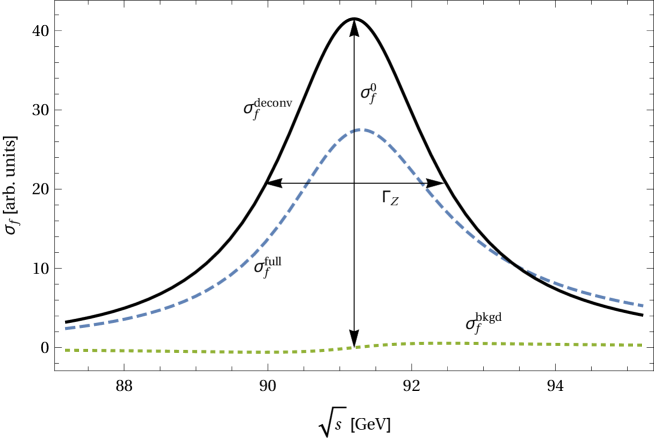
  Figure 11: Illustration of $Z$-pole line-shape observables (not to scale). The dashed line depicts the true line-shape, while the solid line indicates the line-shape after deconvolution of initial-state QED radiation. The dotted line shows the contribution of backgrounds from photon exchange and box contributions to the deconvoluted cross-section.

  It is customary to select the following independent set of quantities to describe this class of observables:

  $$\sigma^{0}_{\rm had} =\sigma[e^{+}e^{-}\to\text{hadrons}]_{s=M_{\rm Z}^{2}},$$ (98)

  $$\Gamma_{Z} =\sum_{f}\Gamma[Z\to f\bar{f}],$$ (99)

  $$R_{\ell} =\Gamma[Z\to\text{hadrons}]/\Gamma[Z\to\ell^{+}\ell^{-}], (\ell=e,\mu,\tau)$$ (100)

  $$R_{q} =\Gamma[Z\to q\bar{q}]/\Gamma[Z\to\text{hadrons}], (q=b,c,s,d,u).$$ (101)

  Here it is implicitly assumed that an $f\bar{f}$ final state always includes contributions from additional real photon and gluon radiation. In this sense, $\sigma[e^{+}e^{-}\to\text{hadrons}]=\sum_{q}\sigma_{q}$.

  Note that $\sigma_{f}(s)$ is not the observable cross-section. The latter, denoted $\sigma^{\rm full}_{f}(s)$ in the following, receives additional contributions from s-channel photon exchange, box contributions and initial-state QED radiation. These have an impact both on the magnitude and the shape of the cross-section as a function of $s$, see Fig. 11 for illustration. To a very good approximation, initial-state QED radiation can be described through a convolution of $\sigma_{f}$ with a radiator function $H(x)$ [144],

  $$\sigma^{\rm full}_{f}(s) =\int_{0}^{1-4m_{f}^{2}/s}dx\;H(x)\,\sigma^{\rm deconv}_{f}(s^{\prime}),\qquad s^{\prime}=s(1-x).$$ (102)

  Including resummed soft-photon and exact ${\cal O}(\alpha^{2})$ contributions, $H(x)$ reads

  $$H(x) =\beta x^{\beta-1}(1+\delta_{1}^{\rm V+S}+\delta_{2}^{\rm V+S})+\delta_{1}^{\rm H}+\delta_{2}^{\rm H},$$ (103)

  $$\beta =\frac{2\alpha}{\pi}(L-1),\qquad L=\log\frac{s}{m_{\rm e}^{2}},$$ (104)

  $$\delta_{1}^{\rm V+S} =\frac{\alpha}{\pi}\biggl{[}\frac{3}{2}L+\frac{\pi^{2}}{3}-2\biggr{]},$$ (105)

  $$\delta_{2}^{\rm V+S} =\Bigl{(}\frac{\alpha}{\pi}\Bigr{)}^{2}\biggl{[}\biggl{(}\frac{9}{8}-\frac{\pi^{2}}{3}\biggr{)}L^{2}+s_{21}L+s_{20}\biggr{]},$$ (106)

  $$\delta_{1}^{\rm H} =\frac{\alpha}{\pi}(L-1)(x-2),$$ (107)

  $$\delta_{2}^{\rm H} =\Bigl{(}\frac{\alpha}{\pi}\Bigr{)}^{2}\bigl{[}h_{22}L^{2}+h_{21}L+h_{20}\bigr{]}.$$ (108)

  The coefficients $s_{21}$, $s_{20}$, $h_{22}$, $h_{21}$ and $h_{20}$ can be found in Ref. [145].

  The deconvoluted cross-section, $\sigma^{\rm deconv}_{f}(s^{\prime})$ contains contributions from s-channel $Z$-boson exchange, s-channel photon exchange, photon-$Z$ interference, and box diagrams. To extract the first part, the remaining pieces are subtracted:

  $$\sigma_{f}(s^{\prime})=\sigma^{\rm deconv}_{f}(s^{\prime})-\sigma^{\gamma}_{f}(s^{\prime})-\sigma^{\gamma\rm Z}_{f}(s^{\prime})-\sigma^{\rm box}_{f}(s^{\prime}).$$ (109)

• Parity-violating asymmetries measured at the $Z$ pole. The forward-backward asymmetry is defined as

  $$A^{f}_{\rm FB} =\frac{\sigma_{f}(\theta<\frac{\pi}{2})-\sigma_{f}(\theta>\frac{\pi}{2})}{\sigma_{f}(\theta<\frac{\pi}{2})+\sigma_{f}(\theta>\frac{\pi}{2})},$$ (110)

  where $\theta$ is the scattering angle between the incoming $e^{-}$ and the outgoing $f$. It can be written as a product of two terms,

  $$A^{f}_{\rm FB} =\tfrac{3}{4}{\cal A}_{e}{\cal A}_{f},$$ (111)

  $${\cal A}_{f} =\frac{1-4|Q_{f}|\sin^{2}\theta_{\rm eff}^{f}}{1-4|Q_{f}|\sin^{2}\theta_{\rm eff}^{f}+8(Q_{f}\sin^{2}\theta_{\rm eff}^{f})^{2}},$$ (112)

  where $\sin^{2}\theta_{\rm eff}^{f}$ is called the effective weak mixing angle. In the presence of polarized electron beams, one can also measure the left-right asymmetry

  $$A^{f}_{\rm LR} =\frac{\sigma_{f}(P_{e}<0)-\sigma_{f}(P_{e}>0)}{\sigma_{f}(P_{e}<0)+\sigma_{f}(P_{e}>0)}={\cal A}_{e}|P_{e}|.$$ (113)

  Here $P_{e}$ is the polarization degree of the incident electrons, with $P_{e}<0$ ($P_{e}>0$) referring to left-handed (right-handed) polarization. Finally, angular and polarization information can be combined to construct

  $$A^{f}_{\rm LR,FB} =\frac{\sigma_{f,\rm LF}-\sigma_{f,\rm LB}-\sigma_{f,\rm RF}+\sigma_{f,\rm RB}}{\sigma_{f,\rm LF}+\sigma_{f,\rm LB}+\sigma_{f,\rm RF}+\sigma_{f,\rm RB}}=\tfrac{3}{4}{\cal A}_{f},$$ (114)

  where $\sigma_{f,\rm LF}=\sigma_{f}(P_{e}<0,\theta<\frac{\pi}{2})$, etc.

The quantities introduced above can be computed within the Standard Model. At tree-level they read, in the limit $m_{f}\ll M_{\rm Z}$,

$$\sigma^{0}_{\rm had} =\sum_{q}\frac{12\pi}{M_{\rm Z}^{2}}\,\frac{\Gamma_{e}\Gamma_{q}}{\Gamma_{\rm Z}^{2}}, \Gamma_{\rm Z} =\sum_{f}\Gamma_{f}, \Gamma_{f} =\frac{N_{c}^{f}\alpha M_{\rm Z}}{24s_{\rm W}^{2}c_{\rm W}^{2}}(1-4s_{\rm W}^{2}|Q_{f}|+8s_{\rm W}^{4}|Q_{f}|^{2}),$$ (115)

$$\Delta r =0, \sin^{2}\theta_{\rm eff}^{f} =s_{\rm W}^{2},$$ (116)

where $N_{c}^{f}=3(1)$ for quarks (leptons) and $s_{\rm W}^{2}=\sin^{2}\theta_{\rm W}$, $c_{\rm W}^{2}=\cos^{2}\theta_{\rm W}$. However, they receive sizable corrections from loop contributions that must be included to match the experimental precision. The loop contributions depend on other Standard Model parameters, most notably $M_{\rm W}$, $M_{\rm H}$, $m_{\rm t}$ and $\alpha_{\rm s}$, so that fits to the electroweak precision data can be used to derive indirect bounds on these parameters.

For a proper theoretical definition of the EWPOs beyond tree-level, one needs to ensure that gauge invariance is preserved at every loop order. For the $Z$-pole observables, this can be achieved by expanding the matrix element for $e^{+}e^{-}\to f\bar{f}$ about the complex pole, $s_{0}\equiv\overline{M}_{\rm Z}^{2}-i\overline{M}_{\rm Z}\overline{\Gamma}_{\rm Z}$ of the $Z$ propagator,

$${\cal M}[e^{+}e^{-}\to f\bar{f}] =\frac{R}{s-s_{0}}+S+(s-s_{0})S^{\prime}+...$$ (117)

Here $\overline{M}_{\rm Z}$ and $\overline{\Gamma}_{\rm Z}$ are the on-shell mass and width of the $Z$ boson. The difference to the unbarred quantities ($M_{\rm Z}$ and $\Gamma_{\rm Z}$) will be explained below. Since the pole is an analytical property of the $S$ matrix, it is gauge-invariant to all orders and can be identified with an observable [146]. It can also be shown explicitly, with the help of Ward or Nielsen identities, that $s_{0}$ as well as the coefficients $R,S,S^{\prime},\dots$ are gauge-parameter independent [147, 148].

When ignoring the non-resonant contributions in (117), it follows that the $s$-dependence of the cross-section near the $Z$ pole is given by the Breit-Wigner function

$$\sigma_{f} \propto\frac{1}{(s-\overline{M}_{\rm Z}^{2})^{2}+\overline{M}_{\rm Z}^{2}\overline{\Gamma}_{\rm Z}^{2}}.$$ (118)

However, in experimental analyses, a different form of the Breit-Wigner line-shape is being used,

$$\sigma_{f} \propto\frac{1}{(s-M_{\rm Z}^{2})^{2}+s^{2}\Gamma_{\rm Z}^{2}/M_{\rm Z}^{2}}.$$ (119)

These two Breit-Wigner forms can be translated into each other with the transformation [149]

$$\overline{M}_{\rm Z} =M_{\rm Z}\big{/}\sqrt{1+\Gamma_{\rm Z}^{2}/M_{\rm Z}^{2}}, \overline{\Gamma}_{\rm Z} =\Gamma_{\rm Z}\big{/}\sqrt{1+\Gamma_{\rm Z}^{2}/M_{\rm Z}^{2}}.$$ (120)

Similar relations hold for the $W$ mass. Numerically, they amount to

$$\overline{M}_{\rm Z} \approx M_{\rm Z}-34\,\,\mathrm{MeV}, \overline{\Gamma}_{\rm Z} \approx\Gamma_{\rm Z}-0.9\,\,\mathrm{MeV},$$ (121)

$$\overline{M}_{\rm W} \approx M_{\rm W}-27\,\,\mathrm{MeV}, \overline{\Gamma}_{\rm W} \approx\Gamma_{\rm W}-0.7\,\,\mathrm{MeV}.$$ (122)

As mentioned above, the non-resonant terms were disregarded in deriving these relations.

Quantities like $G_{\rm F}$, $\sigma^{0}_{\rm had}$, $\Gamma_{\rm Z}$, $R_{\ell}$, $R_{c,b}$, $A^{f}_{\rm FB}$, $A^{f}_{\rm LR}$, and $A^{f}_{\rm LR,FB}$ are frequently used in precision tests of the Standard Model and to derive constraints on new physics. As their definition requires the removal of some photonic corrections, they are called “pseudo-observables,” in contrast to the “true observables” (such as $\Gamma_{\mu}$, $\sigma^{\rm full}_{f}$, etc.). For $G_{\rm F}$, the subtraction of QED corrections is straightforward since these effects can be summarized in the single term $\Delta q$, see eq. (96). On the other hand, for the $Z$-pole observables, the deconvolution of soft and collinear initial-state radiation, see eq. (102), and the subtraction of s-channel photon exchange and box contributions, see eq. (109), is more involved.

There are several public computer codes that carry out this procedure to extract the pseudo-observables from the true observables. ZFitter [150, 151] and TOPAZ0 [152] use analytical expressions for the radiator function $H(x)$, as in eqs. (103) ff. They also permit the implementation of experimental cuts on the invariant mass, angular acceptance or acollinearity of the outgoing fermions.

A potential problem is the fact that these programs do not use a consistent treatment of the complex pole expansion in (117) when performing the subtraction of photon-exchange and box contributions. Nevertheless, it was analyzed in Ref. [115] that the impact of this mismatch is negligible compared to the current experimental uncertainties. It may, however, become relevant for the increased precision of a future high-luminosity $e^{+}e^{-}$ machine (see section 3.6). One should keep in mind that this inconsistency also affects the validity of the translation between the two Breit-Wigner forms in (120). Thus it may be necessary to abandon the form (119) in the future, since only the alternative form (118) has been shown to follow from a self-consistent definition of resonant and non-resonant terms that can be systematically extended to higher precision.

Several other computer codes use Monte-Carlo techniques for the evaluation of external QED radiation. Recent examples are KoralZ [153] and KK-MC [154]. To improve the precision beyond full ${\cal O}(\alpha)$ and resummed leading-logarithmic order, they use exclusive exponentiation [155] based on the Yennie-Frautschi-Suura theory [156] instead of traditional parton showering. See also Ref. [157] for similar considerations of QED radiation in the context of Bhabha scattering.

3.2 Renormalization and input parameters

The loop corrections to the EWPOs contain UV divergences, which must be removed with the help of suitable counterterms. Within the Standard Model, one may choose the masses of all elementary particles, the wave function normalization for asymptotic external states, and the electromagnetic coupling constant as independent quantities, for which counterterms are introduced:

Mass renormalization: $$m_{f,0}=m_{f}+\delta m_{f}, M^{2}_{\rm X,0}=M^{2}_{\rm X}+\delta M^{2}_{\rm X}\quad(X=W,Z,H),$$

Wave function renormalization: $$f^{\rm L}_{0}=\sqrt{1+\delta Z^{f\rm L}}\,f^{\rm L}, f^{\rm R}_{0}=\sqrt{1+\delta Z^{f\rm R}}\,f^{\rm R},$$ (123)

Coupling renormalization: $$e_{0}=(1+\delta Z_{e})e.$$

Here the symbols with (without) subscript 0 denote the bare (renormalized) quantities, and superscripts L,R refer to left- and right-handed fermion fields, respectively. Note that promptly decaying particles, such as the $W$ and $Z$ bosons, cannot be asymptotic external states, and thus no wave function renormalization for these can be defined consistently to all orders in perturbation theory.

One of most commonly used renormalization scheme for the calculation of EWPOs is the “on-shell scheme”. Within this scheme, the electromagnetic coupling constant is defined through the $\gamma f\bar{f}$ vertex in the Thomson limit, where the photon and fermions are on their mass shell. Furthermore, the masses of all elementary Standard Model particles are defined through the pole of their propagator. Note that the masses defined in this way correspond to the barred quantities, $\overline{M}_{\rm X}$, introduced in the previous subsection.

Using these on-shell renormalization conditions, all counterterms can be determined in terms of the one-particle irreducible self-energies

$$\Sigma_{\mu\nu}^{V_{1}V_{2}}(q)=\Bigl{(}g_{\mu\nu}-\frac{q_{\mu}q_{\nu}}{q^{2}}\Bigr{)}\Sigma_{\rm T}^{V_{1}V_{2}}(q^{2})+\frac{q_{\mu}q_{\nu}}{q^{2}}\Sigma_{\rm L}^{V_{1}V_{2}}(q^{2}),\qquad(V_{i}=\rm\gamma,Z,W)$$ (124)

$$\Sigma^{\rm H}(q^{2}),$$ (125)

$$\Sigma^{f}(q)=\makebox[0.34444pt][l]{$q$}/P_{\rm L}\Sigma^{f}_{\rm L(1)}(q^{2})+\makebox[0.34444pt][l]{$q$}/P_{\rm R}\Sigma^{f}_{\rm R(1)}(q^{2})+m_{f}\Sigma^{f}_{\rm S(1)}(q^{2}).$$ (126)

At one-loop order, the relevant on-shell counterterms read

$$\delta\overline{M}_{\rm W}^{2}{}_{(1)} =\text{Re}\bigl{\{}\Sigma_{\rm T(1)}^{\rm WW}(\overline{M}_{\rm W}^{2})\bigr{\}}, \delta Z_{e(1)} =\frac{1}{2}\Sigma^{\gamma\gamma\,\prime}_{\rm T(1)}(0)-\frac{s_{\rm W}}{c_{\rm W}}\,\frac{\Sigma^{\gamma\rm Z}_{\rm T(1)}(0)}{\overline{M}_{\rm Z}^{2}},$$ (127)

$$\delta\overline{M}_{\rm Z}^{2}{}_{(1)} =\text{Re}\bigl{\{}\Sigma_{\rm T(1)}^{\rm ZZ}(\overline{M}_{\rm Z}^{2})\bigr{\}}, \delta Z^{f\rm L}_{(1)} =-\Sigma^{f\rm L}_{(1)}(0),$$ (128)

$$\delta M_{\rm H}^{2}{}_{(1)} =\text{Re}\bigl{\{}\Sigma_{\rm(1)}^{\rm H}(M_{\rm H}^{2})\bigr{\}}, \delta Z^{f\rm R}_{(1)} =-\Sigma^{f\rm R}_{(1)}(0),$$ (129)

$$\delta m_{\rm t}{}_{(1)} =\frac{m_{\rm t}^{2}}{2}\,\text{Re}\bigl{\{}\Sigma_{\rm L}^{f}(m_{\rm t}^{2})+\Sigma_{\rm R}^{f}(m_{\rm t}^{2})+2\Sigma_{\rm S}^{f}(m_{\rm t}^{2})\bigr{\}},$$ (130)

Here the numbers in brackets denote the loop orders, while $\Sigma^{\prime}(p^{2})$ stands for the derivative $\frac{\partial}{\partial p^{2}}\Sigma(p^{2})$. For the EWPOs introduced above, only light fermions ($i.\,e.$ all fermions except the top quark) can appear as external states. Their wave function renormalization can be computed in the limit of vanishing fermion mass, since $m_{f}\ll M_{\rm W},M_{\rm Z}$ for $f=e,\mu\,\tau,u,d,s,c,b$.

To compute two-loop electroweak corrections to the EWPOs introduced above, the following counterterms are also needed at order ${\cal O}(\alpha^{2})$ [117]:

$$\begin{aligned} \delta\overline{M}_{\rm W}^{2}{}_{(2)}=\text{Re}\bigl{\{}\Sigma^{\rm WW}_{\rm T(2)}(\overline{M}_{\rm W}^{2})\bigr{\}}&+\text{Im}\bigl{\{}\Sigma^{\rm WW}_{\rm T(1)}(\overline{M}_{\rm W}^{2})\bigr{\}}\text{Im}\bigl{\{}\Sigma^{\rm WW\,\prime}_{\rm T(1)}(\overline{M}_{\rm W}^{2})\bigr{\}},\end{aligned}$$ (131)

$$\begin{aligned} \delta\overline{M}_{\rm Z}^{2}{}_{(2)}=\text{Re}\bigl{\{}\Sigma^{\rm ZZ}_{\rm T(2)}(\overline{M}_{\rm Z}^{2})\bigr{\}}&+\text{Im}\bigl{\{}\Sigma^{\rm ZZ}_{\rm T(1)}(\overline{M}_{\rm Z}^{2})\bigr{\}}\text{Im}\bigl{\{}\Sigma^{\rm ZZ\,\prime}_{\rm T(1)}(\overline{M}_{\rm Z}^{2})\bigr{\}}\\ &+\frac{1}{\overline{M}_{\rm Z}^{2}}\Bigl{(}\text{Re}\bigl{\{}\Sigma^{\rm\gamma Z}_{\rm T(1)}(\overline{M}_{\rm Z}^{2})\bigr{\}}\Bigr{)}^{2}+\frac{1}{\overline{M}_{\rm Z}^{2}}\Bigl{(}\text{Im}\bigl{\{}\Sigma^{\rm\gamma Z}_{\rm T(1)}(\overline{M}_{\rm Z}^{2})\bigr{\}}\Bigr{)}^{2},\end{aligned}$$ (132)

$$\delta Z^{f\rm L}_{(2)}=-\Sigma^{f\rm L}_{(2)}(0),\qquad\delta Z^{f\rm R}_{(2)}=-\Sigma^{f\rm R}_{(2)}(0),$$ (133)

$$\begin{aligned} \delta Z_{e(2)}=\,&\frac{1}{2}\Sigma^{\gamma\,\prime}_{\rm T(2)}(0)-\frac{s_{\rm W}}{c_{\rm W}}\,\frac{\Sigma^{\gamma\rm Z}_{\rm T(2)}(0)}{\overline{M}_{\rm Z}^{2}}+(\delta Z_{e(1)})^{2}+\frac{1}{8}\bigl{(}\Sigma^{\gamma\,\prime}_{\rm T(1)}(0)\bigr{)}^{2}\\ &+\frac{\Sigma^{\gamma\rm Z}_{\rm T(1)}(0)}{2\overline{M}_{\rm Z}^{2}}\Biggl{[}\frac{1}{s_{\rm W}c_{\rm W}}\,\frac{\delta\overline{M}_{\rm W}^{2}{}_{(1)}}{\overline{M}_{\rm W}^{2}}+\frac{(s_{\rm W}^{2}-c_{\rm W}^{2})}{2s_{\rm W}c_{\rm W}}\,\frac{\delta\overline{M}_{\rm Z}^{2}{}_{(1)}}{\overline{M}_{\rm Z}^{2}}+\frac{\Sigma^{\gamma\rm Z}_{\rm T(1)}(0)}{\overline{M}_{\rm Z}^{2}}\Biggr{]}.\end{aligned}$$ (134)

Here the one-loop formula $\overline{\Gamma}_{\rm Z}{}_{(1)}=\frac{1}{\overline{M}_{\rm Z}}\text{Im}\{\Sigma^{\rm Z}_{\rm T(1)}(\overline{M}_{\rm Z}^{2})\}$ and its equivalent form for the $W$-boson has been used.

The weak gauge couplings can be written as

$$g_{0}=\frac{e_{0}}{s_{\rm W}{}_{,0}}=\frac{e(1+\delta Z_{e})}{s_{\rm W}+\delta s_{\rm W}},\qquad g^{\prime}_{0}=\frac{e_{0}}{c_{\rm W}{}_{,0}}=\frac{e(1+\delta Z_{e})}{c_{\rm W}+\delta c_{\rm W}},$$ (135)

where

$$\frac{\delta s_{\rm W}}{s_{\rm W}}=-\frac{\delta c_{\rm W}}{c_{\rm W}}=\sqrt{1-\frac{\overline{M}_{\rm W}+\delta\overline{M}_{\rm W}}{\overline{M}_{\rm Z}+\delta\overline{M}_{\rm Z}}}-\sqrt{1-\frac{\overline{M}_{\rm W}}{\overline{M}_{\rm Z}}}.$$ (136)

Thus the renormalization of $g$ and $g^{\prime}$ is determined through the renormalization of the electromagnetic couplings and the $W$ and $Z$ masses.

Some of the counterterms contain contributions that are enhanced relative to the remaining electroweak corrections. For instance, the charge counterterm can be written as

$$1+\delta Z_{e} =\frac{1}{\sqrt{1-\Delta\alpha}}+\delta Z_{e,\rm rem}, \Delta\alpha \equiv-\Sigma^{\gamma\gamma\,\prime}_{\rm T,lf}(0)+\frac{\text{Re}\bigl{\{}\Sigma^{\gamma\gamma}_{\rm T,lf}(M_{\rm Z}^{2})\bigr{\}}}{M_{\rm Z}^{2}},$$ (137)

where $\Sigma^{\gamma\gamma}_{\rm T,lf}(q^{2})$ is the contribution to the photon self-energy from light fermions ($e,\mu\,\tau,u,d,s,c,b$). The $\Delta\alpha$ term can be interpreted as a shift of the electromagnetic coupling due to renormalization group running from the scale 0 to $\overline{M}_{\rm Z}^{2}$:

$$\alpha(M_{\rm Z}^{2})=\frac{\alpha}{1-\Delta\alpha}.$$ (138)

It is enhanced by logarithms of the light-fermion masses. For the leptonic part one finds at three-loop order [158]

$$\Delta\alpha_{\rm lept}=0.0314976.$$ (139)

The quark contribution to $\Delta\alpha$, however, receives large non-perturbative QCD corrections, which are difficult to compute from first principles. Instead, this part is typically extracted from experimental data for the cross-section of $e^{+}e^{-}\to\text{hadrons}$ or from tau-lepton decay distributions. Some recent evaluations of $\Delta\alpha_{\rm had}$ are listed in Tab. 2.

Result	Reference
$0.02762\pm 0.00011$	[159]
$0.02750\pm 0.00033$	[160]
$0.02764\pm 0.00014$	[161]
$0.02766\pm 0.00018$	[162]

Table 2: Recent evaluations of $\Delta\alpha_{\rm had}$ from $e^{+}e^{-}$ or $\tau$ decay data.

A second important enhanced contribution is contained in the weak mixing angle counterterm, which at one-loop order can be written as

$$\delta s_{\rm W}{}_{(1)} =\frac{c_{\rm W}^{2}}{2s_{\rm W}}\Delta\rho^{\alpha}_{(1)}+\delta s_{\rm W}{}_{(1),\rm rem}, \Delta\rho^{\alpha}_{(1)} =\frac{\Sigma^{\rm ZZ}_{\rm T(1)}(0)}{M_{\rm Z}^{2}}-\frac{\Sigma^{\rm WW}_{\rm T(1)}(0)}{M_{\rm W}^{2}}=\frac{3\alpha}{16\pi s_{\rm W}^{2}}\;\frac{m_{\rm t}^{2}}{M_{\rm W}^{2}}+\Delta\rho^{\alpha}_{(1),\rm rem}.$$ (140)

The quantity $\Delta\rho^{\alpha}$, called the “$\rho$ parameter,” was first studied in Ref. [163]. It captures the leading custodial-symmetry violating effect due to the Standard Model Yukawa couplings, which in our limit of vanishing light-fermion masses involves only the top Yukawa coupling. When going beyond the Standard Model, the $\rho$ parameter similarly measures the leading custodial-symmetry violating effects of the new particles. Higher-order Standard Model contributions to the $\rho$ parameter were computed in Refs. [164, 165, 166, 167, 168]. Numerically $\Delta\rho\sim 1\%$, but since it enters with a prefactor $\propto s_{\rm W}^{-2}$ in many EWPOs, it can dominate over other loop contributions.

It can be argued that by preforming the perturbation series in powers of $G_{\rm F}/M_{\rm W}^{2}$ rather than in powers of $\alpha$, part of the large $(\Delta\alpha)^{m}(\Delta\rho)^{n-m}$ terms at $n$-loop order are included automatically, thus leading to better convergence of the perturbation series. Furthermore, it was shown [169, 170] that

$$1+\Delta r =\frac{1}{(1-\Delta\alpha)\bigl{(}1+\frac{c_{\rm W}^{2}}{s_{\rm W}^{2}}\Delta\rho^{G}\bigr{)}-\Delta r_{\rm rem}},$$ (141)

$$\sin^{2}\theta_{\rm eff}^{f} =s_{\rm W}^{2}\Bigl{(}1+\frac{c_{\rm W}^{2}}{s_{\rm W}^{2}}\Delta\rho^{G}+\Delta\kappa_{\rm rem}\Bigr{)},$$ (142)

correctly reproduce the $(\Delta\alpha)^{m}(\Delta\rho)^{n-m}$ terms for $n$=2 and for $n$=3, $m{\geq}2$ for these quantities. Here $\Delta\rho^{G}=\frac{3G_{\rm F}m_{\rm t}^{2}}{8\sqrt{2}\pi^{2}}$ and $\Delta r_{\rm rem}$ and $\Delta\kappa_{\rm rem}$ denote the remaining corrections.

However, the resummation of $\Delta\alpha$ and $\Delta\rho$ through these prescriptions is not guaranteed to provide a numerically dominant contribution to the $n$-loop corrections. The reason is that there are large numerical cancellations between different $(\Delta\alpha)^{m}(\Delta\rho)^{n-m}$ terms for fixed $n$. For example, for $n$=3 one obtains

$$\Delta r_{\rm resum,(3)} \begin{array}[t]{l@{\;-\;}c@{\;+\;}c@{\;-\;}c@{}l}=(\Delta\alpha)^{3}&3(\Delta\alpha)^{2}\bigl{(}\tfrac{c_{\rm W}^{2}}{s_{\rm W}^{2}}\Delta\rho^{\alpha}\bigr{)}&6(\Delta\alpha)\bigl{(}\tfrac{c_{\rm W}^{2}}{s_{\rm W}^{2}}\Delta\rho^{\alpha}\bigr{)}^{2}&5\bigl{(}\tfrac{c_{\rm W}^{2}}{s_{\rm W}^{2}}\Delta\rho^{\alpha}\bigr{)}^{3}\\[4.30554pt] \approx(\;2.05&3.40&3.74&1.72&)\times 10^{-4}\\[4.30554pt] \lx@intercol=0.68\times 10^{-4}.\hfil\lx@intercol\end{array}$$ (146)

The sum is comparable in size to some other three-loop contributions.

Another frequently used renormalization scheme is the “$\overline{\text{MS}}$ scheme” [171]. In this scheme, the counterterm consists only of a divergent piece together with some universal parameters. Specifically, the counterterms have the form

$$\delta_{\overline{\text{MS}}}X =C_{X}\bigl{(}\mu^{2}e^{\gamma_{\rm E}}\bigr{)}^{4-D}\,\frac{1}{\epsilon},$$ (147)

where the coefficients $C_{X}$ are to be chosen appropriately to render all physical quantities finite. $\mu$ is a free parameter, which will drop out of physical observables when all orders of perturbation theory are included, but a fixed-order perturbative result has a residual dependence on $\mu$ from missing higher orders. In the calculation of EWPOs, one typically chooses $\mu=M_{\rm Z}$.

As before, one could choose the elementary particle masses and the electromagnetic coupling as the independent quantities $\{X\}$ for which $\overline{\text{MS}}$ counterterms are introduced. Instead, the following set of independent quantities is used more commonly [172, 173, 174]:

1. Fermion masses $\hat{m}_{f}$;

2. Higgs mass $\hat{M}_{\rm H}$;

3. The couplings $\hat{g}$ and $\hat{g}^{\prime}$ or, equivalently, $\hat{s}^{2}=\frac{\hat{g}^{\prime 2}}{\hat{g}^{2}+\hat{g}^{\prime 2}}$ and $\hat{e}=\frac{\hat{g}}{\hat{s}}$.

Here and in the following, the hat ($\hat{X}$) denotes $\overline{\text{MS}}$ quantities. Note that the $\overline{\text{MS}}$ masses in points 1 and 2 depend on the unphysical scale $\mu$ (at finite order in perturbation theory) and do not directly correspond to any observable. In practice, one needs to compute the translation between the $\overline{\text{MS}}$ masses and, say, the on-shell masses at the required order before the results can be compared to experiment. Two-loop results and higher-order QCD contributions for the translation of the top-quark mass were presented in Refs. [176, 24, 175].

The on-shell masses of the $W$ and $Z$ bosons can be computed from $G_{\rm F}$, $\hat{s}^{2}$ and $\hat{e}$ using the relations [172]

$$\overline{M}_{\rm W}^{2} =\frac{\hat{e}^{2}}{4\sqrt{2}G_{\rm F}\hat{s}^{2}}\;\frac{1}{1+\Delta\hat{r}_{\rm W}}, \overline{M}_{\rm Z}^{2} =\frac{\hat{e}^{2}}{4\sqrt{2}G_{\rm F}\hat{s}^{2}(1-\hat{s}^{2})}\;\frac{1}{1+\Delta\hat{r}},$$ (148)

where $\hat{r}_{\rm W}$ and $\delta\hat{r}$ contain the required radiative corrections.

Two-loop results for the $\overline{\text{MS}}$ renormalization of $\hat{e}$, $\hat{s}^{2}$ and $\hat{m}_{\rm t}$, as well as for $\hat{r}_{\rm W}$ were computed in Refs. [177, 176, 178, 179].

The $\overline{\text{MS}}$ scheme has both advantages and disadvantages compared to the on-shell scheme. For instance, the $\overline{\text{MS}}$ scheme is convenient for drawing connections to low-energy physics or to GUT physics through renormalization group running. Furthermore, when employing the $\overline{\text{MS}}$ top mass for computing ${\cal O}(\alpha\alpha_{\rm s}^{n})$ corrections to the $\rho$ parameter, the coefficients for increasing $n$ are much smaller compared to the case when the on-shell mass is used. Specifically, one finds [164, 166, 168]

$$\Delta\rho^{\overline{\text{MS}}}_{\rm QCD} =\frac{3G_{\rm F}\hat{m}_{\rm t}}{8\sqrt{2}\pi^{2}}\biggl{[}-0.193\Bigl{(}\frac{\alpha_{\rm s}}{\pi}\Bigr{)}-2.860\Bigl{(}\frac{\alpha_{\rm s}}{\pi}\Bigr{)}^{2}-1.680\Bigl{(}\frac{\alpha_{\rm s}}{\pi}\Bigr{)}^{3}\biggr{]},$$ (149)

$$\Delta\rho^{\rm OS}_{\rm QCD} =\frac{3G_{\rm F}m_{\rm t}}{8\sqrt{2}\pi^{2}}\biggl{[}-3.970\Bigl{(}\frac{\alpha_{\rm s}}{\pi}\Bigr{)}-14.59\Bigl{(}\frac{\alpha_{\rm s}}{\pi}\Bigr{)}^{2}-93.15\Bigl{(}\frac{\alpha_{\rm s}}{\pi}\Bigr{)}^{3}\biggr{]}.$$ (150)

On the other hand, the $\overline{\text{MS}}$ scheme requires additional translations between $\overline{\text{MS}}$ quantities and actual observables. Furthermore, the $\overline{\text{MS}}$ quantities are in general not guaranteed to be gauge-invariant, although gauge invariance of the $\overline{\text{MS}}$ masses can be achieved in the full Standard Model ($i.\,e.$ without integrating out any heavy particles) through a suitable renormalization of the electroweak vacuum [180].

3.3 QED/QCD and short-distance corrections

When computing radiative corrections to EWPOs, it is convenient to separate them into two categories:

1. Virtual and real QED and QCD radiation from the incoming and outgoing fermions. These contributions contain physical soft and collinear IR divergences that cancel between the virtual and real emission diagrams. They are, furthermore, subject to experimental acceptances and cuts, so that it may be advantageous to treat them with Monte-Carlo techniques.

2. Electroweak corrections involving massive gauge or Higgs bosons. These contributions are IR finite and can be absorbed into short-distance effective couplings, such as $G_{\rm F}$ or the vector and axial-vector couplings of a gauge-boson to a $f\bar{f}$ pair.

It is desirable to factorize the complete set of all radiative corrections into a product of the external radiation part (a) and the massive short-distance part (b). For example, the muon decay rate in eqs. (96) and (97) is written as

$$\Gamma_{\mu} =\frac{\alpha^{2}m_{\mu}^{5}}{384\pi s_{\rm W}^{2}M_{\rm W}^{2}}F\Bigl{(}\frac{m_{\rm e}^{2}}{m_{\mu}^{2}}\Bigr{)}(1+\Delta q)(1+\Delta r)^{2},$$ (151)

where $\Delta q$ represents initial- and final-state QED radiation, while $\Delta r$ denotes massive electroweak corrections. However, in general this factorization is not exact, and there are additional non-factorizable contributions. These first occur at the two-loop level and stem from diagrams with both massless and massive boson exchange. Nevertheless, a factorized form can be recovered by shifting the non-trivial non-factorizable terms into the short-distance part. This can be illustrated by referring again to the example of muon decay:

$$(1+\Delta q)(1+\Delta r_{\rm fact})^{2}+\Delta x_{\rm nonfact}\equiv(1+\Delta q)(1+\Delta r)^{2},$$ (152)

$$\Delta r=\Delta r_{\rm fact}+\frac{\Delta x_{\rm nonfact}}{2(1+\Delta q)(1+\Delta r_{\rm fact})}+{\cal O}\bigl{(}(\Delta x_{\rm nonfact})^{2}\bigr{)},$$ (153)

where the symbol $\Delta x_{\rm nonfact}$ has been introduced to denote the non-factorizable contributions.

For the QED corrections $\Delta q$ defined in this way, complete ${\cal O}(\alpha)$ [181] and ${\cal O}(\alpha^{2})$ [182] contributions are known, including terms that are suppressed by powers of $m_{\rm e}/m_{\mu}$ [183]. As a result, there is a very small relative uncertainty of $6\times 10^{-7}$ for the extracted value of the Fermi constant $G_{\rm F}$.

As far as the short-distance corrections $\Delta r$ are concerned, the full ${\cal O}(\alpha)$ [184], ${\cal O}(\alpha\alpha_{\rm s})$ [164, 185], ${\cal O}(\alpha\alpha_{\rm s}^{2})$ [166, 186] and ${\cal O}(\alpha^{2})$ [116, 117, 187] have been computed. For the calculation of the two-loop electroweak corrections in Refs. [116, 117, 187], some of the numerical techniques described in section 2 have been used. In addition, some leading three- and four-loop corrections in the large-$m_{\rm t}$ limit, that enter through the $\rho$ parameter, are known. These include corrections of order ${\cal O}(\alpha_{\rm t}^{2}\alpha_{\rm s})$, ${\cal O}(\alpha_{\rm t}^{3})$ [167] and ${\cal O}(\alpha_{\rm t}\alpha_{\rm s}^{3})$ [168], where $\alpha_{\rm t}=y_{\rm t}^{2}/(4\pi)$ and $y_{\rm t}$ is the top Yukawa coupling.

Let us now move to the analysis of the $Z$-pole observables. The total $Z$ width, $\overline{\Gamma}_{\rm Z}$, can be obtained from the requirement that $s_{0}\equiv\overline{M}_{\rm Z}^{2}-i\overline{M}_{\rm Z}\overline{\Gamma}_{\rm Z}$ is the pole of the $Z$-boson propagator,

$$(s_{0}-\overline{M}_{\rm Z}^{2})+\Sigma^{\rm Z}_{\rm T}(s_{0})=0,.$$ (154)

Here $\Sigma^{\rm Z}_{\rm T}$, in contrast to $\Sigma^{\rm ZZ}_{\rm T}$ defined in eq. (124), contains contributions from $\gamma$–$Z$ mixing,

$$\Sigma^{\rm Z}_{\rm T}(s)=\Sigma^{\rm ZZ}_{\rm T}(s)-\frac{[\Sigma^{\rm\gamma Z}_{\rm T}(s)]^{2}}{s+\Sigma^{\gamma\gamma}_{\rm T}(s)}.$$ (155)

From the imaginary part of (154) one finds

$$\overline{\Gamma}_{\rm Z} =\frac{1}{\overline{M}_{\rm Z}}\text{Im}\bigl{\{}\Sigma^{\rm Z}_{\rm T}(s_{0})\bigr{\}}$$

$$=\frac{1}{\overline{M}_{\rm Z}}\Bigl{[}\text{Im}\bigl{\{}\Sigma^{\rm Z}_{\rm T}(\overline{M}_{\rm Z}^{2})\bigr{\}}-\overline{M}_{\rm Z}\overline{\Gamma}_{\rm Z}\,\text{Re}\bigl{\{}\Sigma^{\rm Z\prime}_{\rm T}(\overline{M}_{\rm Z}^{2})\bigr{\}}-\tfrac{1}{2}\overline{M}_{\rm Z}^{2}\overline{\Gamma}_{\rm Z}^{2}\text{Im}\bigl{\{}\Sigma^{\rm Z\prime\prime}_{\rm T}(\overline{M}_{\rm Z}^{2})\bigr{\}}+{\cal O}(\overline{\Gamma}_{\rm Z}^{3})\Bigr{]}.$$ (156)

Eq. (156) can be solved recursively for $\overline{\Gamma}_{\rm Z}$. The imaginary part of the self-energy can be related, with the help of the optical theorem, to the decay process $Z\to f\bar{f}$:

$$\text{Im}\,\Sigma^{\rm Z}_{\rm T}=\frac{1}{3\overline{M}_{\rm Z}}\sum_{f}\sum_{\rm spins}\int d\Phi\;\bigl{(}{\cal R}_{\rm V}^{f}|v_{f}|^{2}+{\cal R}_{\rm A}^{f}|a_{f}|^{2}\bigr{)},$$ (157)

where $d\Phi$ is the integration measure for the $f\bar{f}$ phase-space integration. In writing (157), the radiative corrections have been split up, as before, into final-state QED and QCD contributions, which are denoted by the radiator functions ${\cal R}_{\rm V,A}$, and short-distance contributions contained in the effective vector coupling $v_{f}$ and axial vector coupling $a_{f}$ of the $Zf\bar{f}$ vertex. These effective couplings include massive electroweak vertex corrections and $Z$–$\gamma$ mixing contributions. At tree-level, they are given by

$$v_{f(0)} =\frac{e}{s_{\rm W}c_{\rm W}}\bigl{(}\tfrac{1}{2}I_{f}-Q_{f}s_{\rm W}^{2}), a_{f(0)} =\frac{eI_{f}}{2s_{\rm W}c_{\rm W}},$$ (158)

where $I_{f}$ and $Q_{f}$ are the weak isospin and electric charge quantum numbers, respectively.

Inserting (157) into (156) and expanding the electroweak contributions up to next-to-next-to-leading order, one obtains [188, 189]

$$\overline{\Gamma}_{\rm Z} =\sum_{f}\overline{\Gamma}_{f}\,,\qquad\overline{\Gamma}_{f}=\frac{N_{c}^{f}\overline{M}_{\rm Z}}{12\pi}\Bigl{[}{\cal R}_{\rm V}^{f}F_{\rm V}^{f}+{\cal R}_{\rm A}^{f}F_{\rm A}^{f}\Bigr{]}_{s=\overline{M}_{\rm Z}^{2}}\;,$$ (159)

$$F_{\rm V}^{f} =v_{f(0)}^{2}\bigl{[}1-\text{Re}\,\Sigma^{\rm Z\prime}_{\rm T(1)}-\text{Re}\,\Sigma^{\rm Z\prime}_{\rm T(2)}+(\text{Re}\,\Sigma^{\rm Z\prime}_{\rm T(1)})^{2}\bigr{]}+2\,\text{Re}\,(v_{f(0)}v_{f(1)})\bigl{[}1-\text{Re}\,\Sigma^{\rm Z\prime}_{\rm T(1)}\bigr{]}$$

$$\quad+2\,\text{Re}\,(v_{f(0)}v_{f(2)})+|v_{f(1)}|^{2}-\tfrac{1}{2}\overline{M}_{\rm Z}\overline{\Gamma}_{\rm Z}v_{f(0)}^{2}\;\text{Im}\,\Sigma^{\rm Z\prime\prime}_{\rm T(1)}\,,$$ (160)

$$F_{\rm A}^{f} =a_{f(0)}^{2}\bigl{[}1-\text{Re}\,\Sigma^{\rm Z\prime}_{\rm T(1)}-\text{Re}\,\Sigma^{\rm Z\prime}_{\rm T(2)}+(\text{Re}\,\Sigma^{\rm Z\prime}_{\rm T(1)})^{2}\bigr{]}+2\,\text{Re}\,(a_{f(0)}a_{f(1)})\bigl{[}1-\text{Re}\,\Sigma^{\rm Z\prime}_{\rm T(1)}\bigr{]}$$

$$\quad+2\,\text{Re}\,(a_{f(0)}a_{f(2)})+|a_{f(1)}|^{2}-\tfrac{1}{2}\overline{M}_{\rm Z}\overline{\Gamma}_{\rm Z}a_{f(0)}^{2}\;\text{Im}\,\Sigma^{\rm Z\prime\prime}_{\rm T(1)}\,.$$ (161)

The radiator functions ${\cal R}_{\rm V,A}$ are known with QCD corrections up to ${\cal O}(\alpha_{\rm s}^{4})$ [190, 191], QED corrections up to ${\cal O}(\alpha^{2})$ [192] and mixed QED-QCD corrections of ${\cal O}(\alpha\alpha_{\rm s})$ [190]. These have been computed in the limit of massless final-state quarks. Additionally, terms that are suppressed by powers of $m_{q}^{2}/s$ are known up to ${\cal O}(\alpha_{\rm s}^{3})$ [190].

For the short-distance loop corrections in $F^{f}_{\rm V,A}$, entering through $v_{f}$, $a_{f}$ and $\Sigma^{\rm Z}_{\rm T}$, complete electroweak one-loop and fermionic two-loop results have been computed [188, 189]. Here “fermionic” stands for contributions from diagrams with closed fermions loops, which are numerically dominant compared to the “bosonic” contributions. The two-loop electroweak corrections have been computed using numerical loop integration techniques. In addition, the two-loop ${\cal O}(\alpha\alpha_{\rm s})$ corrections are available [164, 185, 193, 194], as well as leading three- and four-loop contributions of ${\cal O}(\alpha_{\rm t}\alpha_{\rm s}^{2})$ [166], ${\cal O}(\alpha_{\rm t}^{2}\alpha_{\rm s})$, ${\cal O}(\alpha_{\rm t}^{3})$ [167] and ${\cal O}(\alpha_{\rm t}\alpha_{\rm s}^{3})$ [168].

The higher-order predictions for the partial widths $\overline{\Gamma}_{f}$ can be used to derive predictions for other pseudo-observables in eqs. (98)–(101):

$$\sigma^{0}_{\rm had} =\sum_{q}\frac{12\pi}{\overline{M}_{\rm Z}^{2}}\;\frac{\overline{\Gamma}_{e}\overline{\Gamma}_{q}}{\overline{\Gamma}_{\rm Z}^{2}}(1+\delta X),$$ (162)

$$R_{\ell} =\frac{\sum_{q}\overline{\Gamma}_{q}}{\sum_{\ell}\overline{\Gamma}_{\ell}},\qquad R_{c}=\frac{\overline{\Gamma}_{c}}{\sum_{q}\overline{\Gamma}_{q}},\qquad R_{b}=\frac{\overline{\Gamma}_{b}}{\sum_{q}\overline{\Gamma}_{q}}.$$ (163)

The correction factor $\delta X$ is obtained by performing the systematic expansion of the matrix element for $e^{+}e^{-}\to f\bar{f}$ about the complex pole $s_{0}$, see eq. (117), and then collecting all terms for $s=\overline{M}_{\rm Z}^{2}$ at the required order. At two-loop order one finds [188]

$$\delta X_{(2)}=-\Bigl{[}(\text{Im}\,\Sigma^{\rm Z\prime}_{\rm T(1)})^{2}+2\overline{M}_{\rm Z}\overline{\Gamma}_{\rm Z}\;\text{Im}\,\Sigma^{\rm Z\prime\prime}_{\rm T(1)}\Bigr{]}_{s=\overline{M}_{\rm Z}^{2}}.$$ (164)

The $Z$-pole asymmetries can also be defined in terms of the effective couplings $v_{f}$ and $a_{f}$, leading to

$$\sin^{2}\theta_{\rm eff}^{f} =\frac{1}{4|Q_{f}|}\biggl{(}1-{\rm Re}\frac{v_{f}}{a_{f}}\biggr{)}=\biggl{(}1-\frac{\overline{M}_{\rm W}^{2}}{\overline{M}_{\rm Z}^{2}}\biggr{)}\,\frac{1-{\rm Re}\{v_{f}/a_{f}\}}{1-v_{f(0)}/a_{f(0)}},$$ (165)

from which the left-right and forward-backward asymmetries can be constructed. The left-right asymmetry, $A^{f}_{\rm LR}$, does not receive any contributions from initial/final-state QED or QCD corrections. The effect of initial- and final-state radiation on the forward-backward asymmetry, $A^{f}_{\rm FB}$, strongly depends on the experimental cuts applied, but it is generally small [195]. Note, however, that the observable forward-backward asymmetry is significantly affected by soft and collinear initial-state radiation, which is already removed in the definition of the pseudo-observable $A^{f}_{\rm FB}$ in terms of the deconvoluted cross-section $\sigma_{f}$ in (110).

The complete electroweak one-loop and two-loop corrections to the leptonic effective weak mixing angle $\sin^{2}\theta_{\rm eff}^{\ell}$ have been computed in Refs. [184, 196] and [118, 115, 112, 129], respectively. As before, numerical loop integration methods were used for the two-loop contributions. Furthermore, mixed electroweak–QCD corrections of ${\cal O}(\alpha\alpha_{\rm s})$ [164, 185] and ${\cal O}(\alpha\alpha_{\rm s}^{2})$ [166, 186] are known, as well as leading contributions entering through the $\rho$ parameter, of order ${\cal O}(\alpha_{\rm t}^{2}\alpha_{\rm s})$, ${\cal O}(\alpha_{\rm t}^{3})$ [167] and ${\cal O}(\alpha_{\rm t}\alpha_{\rm s}^{3})$ [168].

For the quark weak mixing angle $\sin^{2}\theta_{\rm eff}^{q},\;q=u,d,c,s,b$, the situation is similar, except that only fermionic but no bosonic electroweak two-loop corrections are available. Furthermore, the calculation of mixed electroweak–QCD corrections becomes more involved in this case. The additional contributions at order ${\cal O}(\alpha\alpha_{\rm s})$ have been computed in Ref. [193, 194], but only the leading $\rho$-parameter contribution is known at the next order ${\cal O}(\alpha_{\rm t}\alpha_{\rm s}^{2})$ [166].

The use of numerical loop integration techniques has enabled the computation of precise results for the two-loop electroweak contributions to various EWPOs, without needing to resort to any large-mass or small-momentum expansions. However, the numerical evaluation is relatively slow and involves large expressions for the integrands, so that it is difficult to implement these results in this form into other computer codes. Instead they have been made available in the form of convenient parametrization formulae, whose coefficients have been fitted to reproduce the full numerical result over a wide range of values for the input parameters [115, 130, 189, 197]. They have been implemented in the global fitting programs GFitter [198], GAPP [199], in Ref. [200] and partially in ZFitter 6.42 [201].

3.4 Impact of corrections beyond one-loop

Global fits to a set of EWPOs lead to important indirect constraints on physics beyond the Standard Model. See Ref. [202] for recent examples within the context of a variety of new physics models. One can also use a model-independent effective field theory framework to parametrize any deviations from the Standard Model (see Refs. [200, 203] for more information and recent results). At the same time, a fit of the Standard Model to EWPOs tests the theory at the quantum level and leads to indirect constraints on the masses of heavy particles, such as the top-quark and Higgs-boson masses [200, 198, 1].

The inclusion of higher-order corrections in these fits is mandatory to ensure that the results are not subject to systematic errors from missing theory contributions. In Fig. 12, the impact of corrections of different order on the indirect prediction of the Higgs mass, $M_{\rm H}$, from various EWPOs is shown. In each case, the Standard Model prediction of one EWPO is compared to the experimental value in the left side of Tab. 3, using the values on the right side of Tab. 3 for the remaining parametric inputs.

Quantity	Value	Ref.
$M_{\rm W}$	$80.385\pm 0.015\,\,\mathrm{GeV}$	[1]
$\sin^{2}\theta_{\rm eff}^{\ell}$	$0.23153\pm 0.00016$	[204]
$\Gamma_{\rm Z}$	$2.4952\pm 0.0023\,\,\mathrm{GeV}$	[204]

Quantity	Value	Ref.
$G_{\rm F}$	$(11663787\pm 6)\times 10^{-12}\,\,\mathrm{GeV}^{-2}$	[1]
$M_{\rm Z}$	$91.1876\pm 0.0021\,\,\mathrm{GeV}$	[204]
$m_{\rm t}$	$173.24\pm 0.95\,\,\mathrm{GeV}$	[1]
$\alpha_{\rm s}(M_{\rm Z}^{2})$	$0.1185\pm 0.0006$	[1]
$\Delta\alpha_{\rm had}$	$0.02766\pm 0.00018$	[162]

Table 3: Direct measurements of various electroweak precision observables (left); and measurements of other important Standard Model inputs (right).

To produce the data in Fig. 12, the calculations were performed in the on-shell scheme, using an expansion of perturbative electroweak corrections in powers of $\alpha$ (rather than $G_{\rm F}/M_{\rm W}^{2}$). Higher-order corrections are included step-by-step in the following order:

• One-loop corrections, ${\cal O}(\alpha)$;

• Two- and three-loop QCD corrections, ${\cal O}(\alpha\alpha_{\rm s})$ and ${\cal O}(\alpha\alpha_{\rm s}^{2})$;

• Two-loop electroweak corrections from diagrams with two-closed fermion loops, denoted ${\cal O}(\alpha_{\rm 2f})$, which include resummed terms proportional to powers of $\Delta\alpha$ and $\Delta\rho$;

• The remaining two-loop electroweak corrections, denoted ${\cal O}(\alpha_{\rm rem})$, which include the two-loop terms that cannot be obtained from resummation or scheme changes;

• Leading three- and four-loop corrections in the large-$m_{\rm t}$ limit entering through the $\rho$ parameter, ${\cal O}(\alpha_{\rm t}^{2}\alpha_{\rm s})$, ${\cal O}(\alpha_{\rm t}^{3})$ and ${\cal O}(\alpha_{\rm t}\alpha_{\rm s}^{3})$.

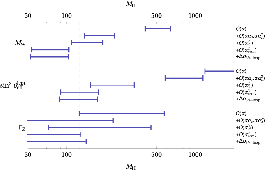
Figure 12: Impact of higher-order corrections on the indirect determination of $M_{\rm H}$ from $M_{\rm W}$ (predicted from $G_{\rm F}$), $\sin^{2}\theta_{\rm eff}^{\ell}$ and $\Gamma_{\rm Z}$. Corrections of different order are cumulatively added as indicated on the right. Here ${\cal O}(\alpha^{2}_{\rm 2f})$ stands for electroweak two-loop contributions with two closed fermion loops, ${\cal O}(\alpha^{2}_{\rm rem})$ denotes the remaining two-loop contributions (with one or no closed fermion loop), and $\Delta\rho_{\rm 3/4-loop}$ are leading 3- and 4-loop corrections of ${\cal O}(\alpha_{\rm t}^{2}\alpha_{\rm s})$, ${\cal O}(\alpha_{\rm t}^{3})$ and ${\cal O}(\alpha_{\rm t}\alpha_{\rm s}^{3})$. The error bars reflect the parametric uncertainty from the input parameters in Tab. 3, but not the theory error from missing higher orders. The dashed line indicates the value $M_{\rm H}=125\,\,\mathrm{GeV}$ from the direct measurement of the Higgs mass.

As evident from the figure, radiative corrections beyond the one-loop level are essential for a reliable test of the Standard Model at the current level of experimental precision. In particular, the non-trivial two-loop electroweak corrections with one or no closed fermion loop, ${\cal O}(\alpha_{\rm rem})$, are sizable and shift the indirect value of $M_{\rm H}$ by about one standard deviation for the most sensitive observables $M_{\rm W}$ and $\sin^{2}\theta_{\rm eff}^{\ell}$. These are the corrections for which the use of numerical loop integration methods has been instrumental. The intrinsic uncertainty from the numerical integration is entirely negligible on the scale shown in the figure. The rather small numerical impact of the leading three- and four-loop corrections, $\Delta\rho_{\rm 3/4-loop}$, is due to the fact the contributions of ${\cal O}(\alpha_{\rm t}^{2}\alpha_{\rm s})$ and ${\cal O}(\alpha_{\rm t}^{3})$ are partially canceled by the ${\cal O}(\alpha_{\rm t}\alpha_{\rm s}^{3})$ terms.

3.5 Theory uncertainties from missing higher-order contributions

As was demonstrated in the previous subsection, multi-loop radiative corrections have a sizable impact on electroweak precision tests. Therefore it is important to estimate the uncertainty from missing higher-order contributions. Unfortunately there is no undisputable method for arriving at this estimate. Some of the common approaches are:

• Collect all relevant prefactors of the most important missing contributions, such as couplings, group factors, particle multiplicities, and mass ratios. This method has been advocated, for example, in Refs. [199, 205].

• When using the $\overline{\text{MS}}$ renormalization scheme, an estimate of missing higher orders may be obtained from varying the renormalization scale, $\mu$, within a certain range, such as $M_{\rm Z}/2<\mu<2M_{\rm Z}$. This idea has been widely used for the evaluation of theory errors from missing QCD corrections, but its application in the electroweak sector stands on less firm footing.

• Another approach is to compare results between different renormalization schemes, for instance between the on-shell and $\overline{\text{MS}}$ schemes. See for example Ref. [206, 207].

• When several orders of a certain quantity have already been computed, one could try to extrapolate to higher orders by assuming that the coefficients of the perturbative series approximately follow a geometric series. There is no formal reason for the validity of this assumption, but in practice it has led to reasonable theory error estimates. This method has been used, for example, in Refs. [117, 115, 189].

In the following, the outcome of these methods will be illustrated with a few examples, and their advantages and disadvantages will be briefly discussed.

Let us begin by examining the use of the prefactor method to estimate the theory error in the prediction of $\Gamma_{\rm Z}$. The most important missing higher order corrections are the bosonic electroweak two-loop contributions, ${\cal O}(\alpha_{\rm bos})$, three-loop contributions of orders $\alpha^{3}$, $\alpha^{2}\alpha_{\rm s}$ and $\alpha\alpha_{\rm s}^{2}$, and four-loop contributions of order $\alpha\alpha_{\rm s}^{3}$. For all these contributions except the ${\cal O}(\alpha_{\rm bos})$ terms, the leading terms in the large-$m_{\rm t}$ limit are already known, so the uncertainty pertains only to the remaining, non-enhanced terms. The following estimates are obtained with the prefactor method:

$${\cal O}(\alpha_{\rm bos})\sim\Gamma_{\rm Z}\alpha^{2}\approx 0.13\,\,\mathrm{MeV},$$

$${\cal O}(\alpha^{3})-{\cal O}(\alpha_{\rm t}^{3})\sim\Gamma_{\rm Z}\alpha\alpha_{\rm t}^{2}\approx 0.12\,\,\mathrm{MeV},$$

$${\cal O}(\alpha^{2}\alpha_{\rm s})-{\cal O}(\alpha_{\rm t}^{2}\alpha_{\rm s})\sim\Gamma_{\rm Z}\,\frac{\alpha\alpha_{\rm t}n_{q}}{\pi}\alpha_{\rm s}(m_{\rm t})\approx 0.23\,\,\mathrm{MeV},$$ (166)

$${\cal O}(\alpha\alpha_{\rm s}^{2})-{\cal O}(\alpha_{\rm t}\alpha_{\rm s}^{2})\sim\Gamma_{\rm Z}\,\frac{\alpha n_{q}}{\pi}\alpha_{\rm s}^{2}(m_{\rm t})\approx 0.35\,\,\mathrm{MeV},$$

$${\cal O}(\alpha\alpha_{\rm s}^{3})-{\cal O}(\alpha_{\rm t}\alpha_{\rm s}^{3})\sim\Gamma_{\rm Z}\,\frac{\alpha n_{q}}{\pi}\alpha_{\rm s}^{3}(m_{\rm t})\approx 0.04\,\,\mathrm{MeV}.$$

Alternatively, one may estimate the theory error for $\Gamma_{\rm Z}$ using the geometric series extrapolation method. As mentioned above, we are only interested in the missing contributions of orders $\alpha^{3}$, $\alpha^{2}\alpha_{\rm s}$, $\alpha\alpha_{\rm s}^{2}$ and $\alpha\alpha_{\rm s}^{3}$ beyond the known leading large-$m_{\rm t}$ part. Consequently, the leading large-$m_{\rm t}$ part must also be excluded for the lower order which is used as reference for the extrapolation. In this way, one obtains [189]

$${\cal O}(\alpha_{\rm bos})\sim[{\cal O}(\alpha_{\rm bos})]^{2}\approx 0.10\,\,\mathrm{MeV},$$

$${\cal O}(\alpha^{3})-{\cal O}(\alpha_{\rm t}^{3})\sim\frac{{\cal O}(\alpha^{2})}{{\cal O}(\alpha)}\,[{\cal O}(\alpha^{2})-{\cal O}(\alpha_{\rm t}^{2})]\approx 0.26\,\,\mathrm{MeV},$$

$${\cal O}(\alpha^{2}\alpha_{\rm s})-{\cal O}(\alpha_{\rm t}^{2}\alpha_{\rm s})\sim\frac{{\cal O}(\alpha\alpha_{\rm s})}{{\cal O}(\alpha)}\,[{\cal O}(\alpha^{2})-{\cal O}(\alpha_{\rm t}^{2})]\approx 0.30\,\,\mathrm{MeV},$$ (167)

$${\cal O}(\alpha\alpha_{\rm s}^{2})-{\cal O}(\alpha_{\rm t}\alpha_{\rm s}^{2})\sim\frac{{\cal O}(\alpha\alpha_{\rm s})}{{\cal O}(\alpha)}\,[{\cal O}(\alpha\alpha_{\rm s})-{\cal O}(\alpha_{\rm t}\alpha_{\rm s})]\approx 0.23\,\,\mathrm{MeV},$$

$${\cal O}(\alpha\alpha_{\rm s}^{3})-{\cal O}(\alpha_{\rm t}\alpha_{\rm s}^{3})\sim\frac{{\cal O}(\alpha\alpha_{\rm s}^{2})}{{\cal O}(\alpha)}\,[{\cal O}(\alpha\alpha_{\rm s})-{\cal O}(\alpha_{\rm t}\alpha_{\rm s})]\approx 0.035\,\,\mathrm{MeV}.$$

By comparing (166) and (167), one can see that both methods lead to comparable estimates, although there are sizable differences for certain individual contributions. Adding all contributions in quadrature, the total error is estimated to be $\delta_{\rm th}\Gamma_{\rm Z}\sim 0.5\,\,\mathrm{MeV}$.

The scale variation method has mostly been applied for the estimation of higher-order QCD corrections to EWPOs. In Ref. [117] it has been used to estimate the ${\cal O}(\alpha^{2}\alpha_{\rm s})$ and ${\cal O}(\alpha\alpha_{\rm s}^{3})$ contributions to $M_{\rm W}$ to amount to $\approx 3.8\,\,\mathrm{MeV}$ and $\approx 0.7\,\,\mathrm{MeV}$, respectively. Since then, the leading large-$m_{\rm t}$ contributions at order $\alpha_{\rm t}^{2}\alpha_{\rm s}$ and $\alpha_{\rm t}\alpha_{\rm s}^{3}$ have been calculated [167, 168], yielding about 2 MeV each when using the on-shell definition for the top-quark mass. Thus the magnitude of the ${\cal O}(\alpha^{2}\alpha_{\rm s})$ contributions has been properly estimated from the scale variation, whereas the ${\cal O}(\alpha\alpha_{\rm s}^{3})$ contributions were somewhat underestimated. This may be partially due to the use of the on-shell top-quark mass, whereas better estimates may be obtained when consistently using $\overline{\text{MS}}$ renormalization for all quantities that receive QCD corrections.

Finally, the analysis of scheme variation has also been used to evaluate the impact of missing higher-order corrections. In Ref. [207, 208], approximate results for the electroweak two-loop corrections to $M_{\rm W}$, $\sin^{2}\theta_{\rm eff}^{\ell}$ and $\Gamma_{\ell}$ were computed in the $\overline{\text{MS}}$ and the on-shell scheme. These results incorporated the leading, ${\cal O}(\alpha^{2}m_{\rm t}^{4}/MW^{4})$, and next-to-leading, ${\cal O}(\alpha^{2}m_{\rm t}^{2}M_{\rm W}^{2})$, contributions in an expansion for large values of $m_{\rm t}$, besides resummed terms involving $\Delta\alpha$. The $\overline{\text{MS}}$ and on-shell results can be compared to estimate the remaining two-loop electroweak contributions. The observed differences were $\delta M_{\rm W}\approx 2\,\,\mathrm{MeV}$, $\delta\sin^{2}\theta_{\rm eff}^{\ell}\approx 3\times 10^{-5}$ and $\delta\Gamma_{\ell}\approx 0.001\,\,\mathrm{MeV}$ for $M_{\rm H}\sim 100\,\,\mathrm{GeV}$. Later, explicit results for the remaining ${\cal O}(\alpha^{2})$ contributions were obtained, resulting in significantly larger numerical effects: $\delta M_{\rm W}\approx 4\,\,\mathrm{MeV}$ [116, 117], $\delta\sin^{2}\theta_{\rm eff}^{\ell}\gtrsim 4\times 10^{-5}$ [118, 115] and $\delta\Gamma_{\ell}\approx 0.02\,\,\mathrm{MeV}$ [189].

This underestimation of the theory error may not be entirely surprising since the difference between renormalization schemes is part of the missing higher-order corrections, but there is no strong reason to assume that it is the numerically dominant part. More recently, the complete two-loop corrections to the prediction of the $W$ mass have been computed both in the on-shell and $\overline{\text{MS}}$ schemes. The difference between the results in Ref. [179] and in the arXiv update of Ref. [197] (hep-ph/0311186v2) can be taken as an estimate of the missing three-loop contributions. It amounts to 4–5 MeV, in reasonable agreement with other estimates of the missing higher-order contributions [197].

3.6 Future projections

Table 4 gives a summary of the estimated theory uncertainty for several important electroweak precision observables, compared with their current experimental precision from measurements at LEP, SLC and Tevatron. In all cases, the theory error is smaller than the experimental uncertainty by a factor of a few, which is a desirable situation since it implies a subdominant impact from ambiguities in defining and evaluating the theoretical uncertainty (see previous subsection).

Quantity	Theory error	Exp. error
$M_{\rm W}$ [MeV]	4	15
$\sin^{2}\theta_{\rm eff}^{\ell}$ [$10^{-5}$]	4.5	16
$\Gamma_{\rm Z}$ [MeV]	0.5	2.3
$R_{b}$ [$10^{-5}$]	15	66

Table 4: Estimated theory error of available predictions for several important electroweak precision observables (from Refs. [197, 115, 189]), compared to the current experimental error (from Refs. [204, 1]).

There are several proposals for future high-luminosity $e^{+}e^{-}$ colliders, which are expected to measure electroweak precision observables, in particular $Z$-pole observables and the $W$ mass, to significantly higher precision. The first proposal, the International Linear Collider (ILC), is planned to be a linear $e^{+}e^{-}$ machine with adjustable center-of-mass energy in the range $\sqrt{s}\sim 90\dots 500\,\,\mathrm{GeV}$, extendable to 1 TeV [209, 210]. It can accommodate polarized $e^{-}$ and $e^{+}$ beams and is expected to collect more than 50 fb^-1 of data near the $Z$ pole and 100 fb^-1 near the $W$ pair production threshold. An alternative proposal, the Future Circular Collider (FCC-ee), is based on a 80–100 km circumference accelerator ring with $\sqrt{s}\sim 90\dots 350\,\,\mathrm{GeV}$ [211]. It has the potential to generate several ab^-1 of data near the $Z$ pole and a comparable amount at the $WW$ threshold. Finally, there is the Circular Electron-Positron Collider (CEPC) proposal [212], which is also a ring collider with 50–70 km circumference and $\sqrt{s}\sim 90\dots 250\,\,\mathrm{GeV}$. Its target luminosities are 150 fb^-1 at the $Z$ pole and 100 fb^-1 near the $WW$ threshold.

Quantity	ILC	FCC-ee	CEPC	Projected theory error
$M_{\rm W}$ [MeV]	3–4	1	3	1
$\sin^{2}\theta_{\rm eff}^{\ell}$ [$10^{-5}$]	1	0.6	2.3	1.5
$\Gamma_{\rm Z}$ [MeV]	0.8	0.1	0.5	0.2
$R_{b}$ [$10^{-5}$]	14	6	17	5–10

Table 5: Estimated experimental precision for several important electroweak precision observables at future $e^{+}e^{-}$ colliders [210, 213, 211, 214, 212] (no theory uncertainties included, see text). In the last column, the estimated error for the theoretical predictions of these quantities is given, under the assumption that ${\cal O}(\alpha\alpha_{\rm s}^{2})$, fermionic ${\cal O}(\alpha^{2}\alpha_{\rm s})$, fermionic ${\cal O}(\alpha^{3})$, and leading four-loop corrections entering through the $\rho$-parameter will become available [215].

All of these machines will significantly improve the experimental uncertainty for the determination of electroweak precision observables (EWPOs), see Tab. 5 [210, 213, 211, 214, 212]. As a consequence, the experimental error for many quantities will become comparable or even subdominant compared to the theory error, from missing higher-order corrections, in the prediction of these quantities within the Standard Model. Therefore it will be necessary to compute three-loop and even leading four-loop corrections to be able to take full advantage of the potential of these future accelerators. In Ref. [215], it has been estimated by how much the theory error may be expected to be reduced if the complete ${\cal O}(\alpha\alpha_{\rm s}^{2})$ corrections, the fermionic ${\cal O}(\alpha^{2}\alpha_{\rm s})$ and ${\cal O}(\alpha^{3})$ corrections, and the leading four-loop corrections in the large-$m_{\rm t}$ limit will become available. This estimate is based on the geometric series extrapolation method discussed in the previous subsection, and only provides an order-of-magnitude projection. The results are shown in the last column of Tab. 5.

On the technical side, the calculation of these corrections will include three-loop self-energy and vertex integrals with many different masses in the propagators. It appears highly unlikely that they can be tackled with analytical methods. In some cases, in particular diagrams involving top-quark propagators, asymptotic expansion techniques may be helpful to arrive at a result with sufficient accuracy. Alternatively, and for the remaining cases, numerical integration methods will need to be employed. None of the techniques described in this review can be immediately deployed to this problem, but further developments and improvements in numerical efficiency and convergence will be required to carry out these calculations.

In addition, theoretical improvements will be necessary for the processes that are being used to extract the relevant Standard Model input parameters. These include $M_{\rm W}$, which can be determined from the $e^{+}e^{-}\to W^{+}W^{-}$ cross-section near threshold, and $m_{\rm t}$, which can be determined from the $e^{+}e^{-}\to t\bar{t}$ cross-section near threshold. A lot of effort has been invested into precision calculations for the $t\bar{t}$ cross-section, culminating in the recent completion of full ${\cal O}(\alpha_{\rm s}^{3})$ [216] and partial ${\cal O}(\alpha)$ electroweak [217] corrections. Together with future improvements in the determination of $\alpha_{\rm s}$, this appears to enable a determination of $m_{\rm t}$ from $e^{+}e^{-}\to t\bar{t}$ with a theory error of about 50 MeV [218].

On the other hand, a much more ambitious precision target of 1 MeV is envisioned for $M_{\rm W}$ at FCC-ee, see Tab. 5. On the theory side, this will require the inclusion of multi-loop electroweak corrections for the prediction of $e^{+}e^{-}\to W^{+}W^{-}$ near threshold. The current state of the art includes complete one-loop electroweak corrections for $W$-boson pair production and decay with off-shell effects [219], as well as two-loop contributions that are enhanced by the Coulomb singularity from soft photon exchange [220]. The theory uncertainty is estimated to be $\delta_{\rm th}M_{\rm W}\sim 3\,\,\mathrm{MeV}$, which is not sufficient for the FCC-ee and CEPC precision targets. The most important steps for improving the theoretical precision are the calculation of full ${\cal O}(\alpha^{2})$ electroweak corrections to on-shell $W$-boson pair production ($e^{+}e^{-}\to W^{+}W^{-}$) and to on-shell $W$-boson decay ($W\to f\bar{f}^{\prime}$), which are building blocks for the effective field theory framework in Refs. [220, 221]. Since these contributions depend on many independent mass and momentum scales, it again is likely that numerical loop integration methods are the most promising avenue towards dealing with these challenges.

Another important quantity is the shift in the electromagnetic fine structure constant from hadronic contributions, $\Delta\alpha_{\rm had}$. It can be extracted from data on $e^{+}e^{-}\to\text{hadrons}$, which may be improved in the future by, $e.\,g.$, radiative return events measured at Belle-II [222]. Alternatively, $\alpha(M_{\rm Z}^{2})$ could be measured directly at a very-high-luminosity $e^{+}e^{-}$ machine, such as FCC-ee, by taking data at a few GeV above and below the $Z$ peak [223]. This approach will require very precise Standard Model predictions for $e^{+}e^{-}\to f\bar{f}$, including fermionic three-loop vertex and box corrections. This is another example where numerical integration techniques can play an essential role.

4 Summary

Since the 1980s, results from particle physics experiments have reached a level of precision that makes the consideration of radiative corrections a necessary element of many experimental analyses and interpretations thereof. With increasing number of loops and increasing number of mass and momentum scales, it becomes more difficult to compute these corrections analytically. Thus, both from a conceptual and practical point of view, one needs to resort to non-analytical methods for the evaluation of multi-loop multi-scale problems. Broadly speaking, these can be divided into two categories: asymptotic expansions and numerical integration techniques.

The asymptotic expansion technique aims to write a loop amplitude as a series in powers of a suitable small parameter, such as a small mass or momentum scale, the inverse of a large mass or momentum scale, or a small mass difference. The coefficients of this series are simpler loop integrals, which are more amenable for analytical evaluation. An asymptotic expansion may also be performed in terms of more than one expansion parameter, in order to simplify the analytics even further. By computing ${\cal O}(10)$ terms for each expansion parameter, one can obtain sufficiently accurate results for many practical purposes. Nevertheless, by its very nature, this method delivers only approximate results. In principle, the quality of the approximation can be systematically improved by including more terms of the series, but the computational complexity grows significantly with each additional term.

Numerical integration techniques, on the other hand, aim to evaluate a given loop amplitude without any specific approximation, by performing some subset or all integrations of a multi-dimensional integral numerically. Depending on the chosen technique, the numerical integration may be carried out directly in the loop momentum space, or one may transform the integral to a different set of variables, such as Feynman parameters. In any case, a successful numerical integration technique will be subject to three general requirements: (i) a method for the removal or regularization of UV and IR singularities; (ii) sufficiently fast convergence of the numerical integration for a range of values of the input parameters; and (iii) applicability to a variety of physical processes with different numbers of external legs and different types of particles in the loops.

In section 2, a variety of different numerical loop integration techniques have been reviewed, and their approaches to addressing the aforementioned requirements have been discussed. Due to the contribution of many researchers, tremendous progress in the development and improvement of numerical integration techniques has been achieved over the last 20 years. Nevertheless, no single technique is applicable to any arbitrary multi-loop multi-scale problem. Instead, different techniques have advantages and disadvantages for certain applications.

For instance, sector decomposition and Mellin-Barnes representations provide a general and fully automatizable algorithm for the extraction of UV and IR divergences from arbitrary multi-loop integrals. However, they have problems with reaching high numerical stability and precision in many physical applications. At the other extreme are techniques like dispersion relations, the Bernstein-Tkachov method, and differential equations, which are capable of producing high-precision numerical results, but which require substantial work to adapt them to a new class of processes. Here a class of processes is characterized by the number of loops and external legs, as well as the types of subloops that can appear in a given Feynman diagram.

The availability of a variety of different numerical loop integration techniques has led to tremendous progress in the computation of difficult higher-loop contributions. As a concrete example, the computation of electroweak two-loop corrections to the most important electroweak precision observables has been reviewed in section 3. These observables are the $W$-mass, which can be predicted from the muon decay rate, and $Z$-pole observables, such as the peak $Z$ production cross-section, the total $Z$ width and branching ratios, and various parity-breaking asymmetries.

These corrections can be computed in different renormalization schemes, which differ in the higher-order terms that are implicitly resummed. Due to cancellations between different terms, the resummed terms are generically numerically small, so that there is no phenomenologically motivated advantage of one renormalization scheme over another. For practical purposes, the radiative corrections are factorized into initial- and final-state QED and QCD corrections, which include real emission contributions, and massive electroweak corrections, which are free of physical IR divergences. Due to the efforts of many groups, high-precision results are available for both of these categories, resulting in an estimated theory error that is safely below the experimental uncertainties for all relevant electroweak precision observables.

The estimation of theory uncertainties has been discussed in some detail in section 3.5, with the conclusion that no single method is fully reliable, but instead it is advantageous to compare the outcomes of different error estimation methods. These issues are important in the context of planned future high-luminosity $e^{+}e^{-}$ colliders that are projected to obtain electroweak precision data with substantially improved precision. To match the projected experimental precision, new theory calculations will be necessary, including three-loop electroweak corrections. Numerical methods will likely play an essential role in achieving this goal. However, none of the available methods is immediately applicable to this task, but new developments and improvements will be needed.

References

- [1] K. A. Olive et al. [Particle Data Group Collaboration], Chin. Phys. C 38 (2014) 090001.
- [2] C. G. Bollini and J. J. Giambiagi, Nuovo Cim. B 12 (1972) 20; J. F. Ashmore, Lett. Nuovo Cim. 4 (1972) 289; G. ’t Hooft and M. J. G. Veltman, Nucl. Phys. B 44 (1972) 189; G. Leibbrandt, Rev. Mod. Phys. 47 (1975) 849.
- [3] G. Passarino and M. J. G. Veltman, Nucl. Phys. B 160 (1979) 151.
- [4] G. Weiglein, R. Scharf and M. Böhm, Nucl. Phys. B 416 (1994) 606 [hep-ph/9310358].
- [5] K. G. Chetyrkin and F. V. Tkachov, Nucl. Phys. B 192 (1981) 159.
- [6] S. Laporta and E. Remiddi, Phys. Lett. B 379 (1996) 283 [hep-ph/9602417]; S. Laporta, Int. J. Mod. Phys. A 15 (2000) 5087 [hep-ph/0102033].
- [7] T. Gehrmann and E. Remiddi, Nucl. Phys. B 580 (2000) 485 [hep-ph/9912329].
- [8] S. G. Gorishnii, S. A. Larin, L. R. Surguladze and F. V. Tkachov, Comput. Phys. Commun. 55 (1989) 381.
- [9] C. Anastasiou and A. Lazopoulos, JHEP 0407 (2004) 046 [hep-ph/0404258].
- [10] A. V. Smirnov, JHEP 0810 (2008) 107 [arXiv:0807.3243 [hep-ph]]; A. V. Smirnov, Comput. Phys. Commun. 189 (2014) 182 [arXiv:1408.2372 [hep-ph]].
- [11] C. Studerus, Comput. Phys. Commun. 181 (2010) 1293 [arXiv:0912.2546 [physics.comp-ph]]; A. von Manteuffel and C. Studerus, arXiv:1201.4330 [hep-ph].
- [12] R. N. Lee, arXiv:1212.2685 [hep-ph]; R. N. Lee, J. Phys. Conf. Ser. 523 (2014) 012059 [arXiv:1310.1145 [hep-ph]].
- [13] P. A. Baikov, Phys. Lett. B 385 (1996) 404 [hep-ph/9603267]; P. A. Baikov, Nucl. Instrum. Meth. A 389 (1997) 347 [hep-ph/9611449].
- [14] P. A. Baikov, Phys. Lett. B 634 (2006) 325 [hep-ph/0507053].
- [15] O. V. Tarasov, Phys. Rev. D 54 (1996) 6479 [hep-th/9606018]; O. V. Tarasov, Nucl. Phys. B 502 (1997) 455 [hep-ph/9703319].
- [16] C. Anastasiou, E. W. N. Glover and C. Oleari, Nucl. Phys. B 575 (2000) 416 [Erratum-ibid. 585 (2000) 763] [hep-ph/9912251]; C. Anastasiou, T. Gehrmann, C. Oleari, E. Remiddi and J. B. Tausk, Nucl. Phys. B 580 (2000) 577 [hep-ph/0003261].
- [17] Z. Bern, L. J. Dixon, D. C. Dunbar and D. A. Kosower, Nucl. Phys. B 425 (1994) 217 [hep-ph/9403226]; R. Britto, F. Cachazo and B. Feng, Nucl. Phys. B 725 (2005) 275 [hep-th/0412103].
- [18] G. Ossola, C. G. Papadopoulos and R. Pittau, Nucl. Phys. B 763 (2007) 147 [hep-ph/0609007]; C. Anastasiou, R. Britto, B. Feng, Z. Kunszt and P. Mastrolia, Phys. Lett. B 645 (2007) 213 [hep-ph/0609191]; W. T. Giele, Z. Kunszt and K. Melnikov, JHEP 0804 (2008) 049 [arXiv:0801.2237 [hep-ph]]; R. K. Ellis, W. T. Giele, Z. Kunszt and K. Melnikov, Nucl. Phys. B 822 (2009) 270 [arXiv:0806.3467 [hep-ph]].
- [19] C. F. Berger, Z. Bern, L. J. Dixon, F. Febres Cordero, D. Forde, H. Ita, D. A. Kosower and D. Maitre, Phys. Rev. D 78 (2008) 036003 [arXiv:0803.4180 [hep-ph]]; W. T. Giele and G. Zanderighi, JHEP 0806 (2008) 038 [arXiv:0805.2152 [hep-ph]]; G. Bevilacqua, M. Czakon, M. V. Garzelli, A. van Hameren, A. Kardos, C. G. Papadopoulos, R. Pittau and M. Worek, Comput. Phys. Commun. 184 (2013) 986 [arXiv:1110.1499 [hep-ph]]; V. Hirschi, R. Frederix, S. Frixione, M. V. Garzelli, F. Maltoni and R. Pittau, JHEP 1105 (2011) 044 [arXiv:1103.0621 [hep-ph]]; F. Cascioli, P. Maierhofer and S. Pozzorini, Phys. Rev. Lett. 108 (2012) 111601 [arXiv:1111.5206 [hep-ph]]; S. Agrawal, T. Hahn and E. Mirabella, J. Phys. Conf. Ser. 368 (2012) 012054 [arXiv:1112.0124 [hep-ph]]; S. Badger, B. Biedermann, P. Uwer and V. Yundin, Comput. Phys. Commun. 184 (2013) 1981 [arXiv:1209.0100 [hep-ph]]; G. Cullen et al., Eur. Phys. J. C 74 (2014) 8, 3001 [arXiv:1404.7096 [hep-ph]].
- [20] R. K. Ellis, Z. Kunszt, K. Melnikov and G. Zanderighi, Phys. Rept. 518 (2012) 141 [arXiv:1105.4319 [hep-ph]].
- [21] Z. Bern, L. J. Dixon and D. A. Kosower, JHEP 0001 (2000) 027 [hep-ph/0001001]; Z. Bern, J. J. M. Carrasco, H. Johansson and D. A. Kosower, Phys. Rev. D 76 (2007) 125020 [arXiv:0705.1864 [hep-th]]; J. Gluza, K. Kajda and D. A. Kosower, Phys. Rev. D 83 (2011) 045012 [arXiv:1009.0472 [hep-th]]; P. Mastrolia and G. Ossola, JHEP 1111 (2011) 014 [arXiv:1107.6041 [hep-ph]]; D. A. Kosower and K. J. Larsen, Phys. Rev. D 85 (2012) 045017 [arXiv:1108.1180 [hep-th]]; S. Badger, H. Frellesvig and Y. Zhang, JHEP 1204 (2012) 055 [arXiv:1202.2019 [hep-ph]]; P. Mastrolia, E. Mirabella, G. Ossola and T. Peraro, Phys. Lett. B 718 (2012) 173 [arXiv:1205.7087 [hep-ph]]; H. Johansson, D. A. Kosower and K. J. Larsen, Phys. Rev. D 87 (2013) 2, 025030 [arXiv:1208.1754 [hep-th]]; B. Feng and R. Huang, JHEP 1302 (2013) 117 [arXiv:1209.3747 [hep-ph]].
- [22] R. J. Gonsalves, Phys. Rev. D 28 (1983) 1542; G. Kramer and B. Lampe, J. Math. Phys. 28 (1987) 945; W. L. van Neerven, Nucl. Phys. B 268 (1986) 453.
- [23] M. Beneke, A. Signer and V. A. Smirnov, Phys. Rev. Lett. 80 (1998) 2535 [hep-ph/9712302]; A. Czarnecki and K. Melnikov, Phys. Rev. Lett. 87 (2001) 013001 [hep-ph/0012053].
- [24] K. G. Chetyrkin and M. Steinhauser, Nucl. Phys. B 573 (2000) 617 [hep-ph/9911434].
- [25] E. Panzer, JHEP 1403 (2014) 071 [arXiv:1401.4361 [hep-th]]; E. Panzer, Ph.D. thesis, Humboldt University Berlin (2015) [arXiv:1506.07243 [math-ph]].
- [26] A. I. Davydychev and J. B. Tausk, Nucl. Phys. B 397 (1993) 123.
- [27] V. A. Smirnov, Phys. Lett. B 460 (1999) 397 [hep-ph/9905323]; J. B. Tausk, Phys. Lett. B 469 (1999) 225 [hep-ph/9909506]; G. Heinrich and V. A. Smirnov, Phys. Lett. B 598 (2004) 55 [hep-ph/0406053].
- [28] V. A. Smirnov, Phys. Lett. B 567 (2003) 193 [hep-ph/0305142].
- [29] A. V. Kotikov, Phys. Lett. B 254 (1991) 158; A. V. Kotikov, Phys. Lett. B 267 (1991) 123; A. V. Kotikov, Phys. Lett. B 259 (1991) 314; E. Remiddi, Nuovo Cim. A 110 (1997) 1435 [hep-th/9711188].
- [30] J. M. Henn, Phys. Rev. Lett. 110 (2013) 251601 [arXiv:1304.1806 [hep-th]].
- [31] V. A. Smirnov, “Feynman integral calculus,” Springer (Berlin, Germany) (2006).
- [32] E. Remiddi and J. A. M. Vermaseren, Int. J. Mod. Phys. A 15 (2000) 725 [hep-ph/9905237].
- [33] A. B. Goncharov, Math. Res. Lett. 5 (1998), 497 [arXiv:1105.2076 [math.AG]].
- [34] V. A. Smirnov, Mod. Phys. Lett. A 10 (1995) 1485 [hep-th/9412063].
- [35] M. Beneke and V. A. Smirnov, Nucl. Phys. B 522 (1998) 321 [hep-ph/9711391].
- [36] V. A. Smirnov, Phys. Lett. B 465 (1999) 226 [hep-ph/9907471]; B. Jantzen, JHEP 1112 (2011) 076 [arXiv:1111.2589 [hep-ph]].
- [37] F. Jegerlehner, M. Y. Kalmykov and O. Veretin, Nucl. Phys. B 641 (2002) 285 [hep-ph/0105304]; M. Czakon, M. Awramik and A. Freitas, Nucl. Phys. Proc. Suppl. 157 (2006) 58 [hep-ph/0602029].
- [38] A. Ghinculov and J. J. van der Bij, Nucl. Phys. B 436 (1995) 30 [hep-ph/9405418].
- [39] A. Ghinculov and Y. P. Yao, Nucl. Phys. B 516 (1998) 385 [hep-ph/9702266].
- [40] A. Ghinculov, Phys. Lett. B 337 (1994) 137 [Phys. Lett. B 346 (1995) 426] [hep-ph/9405394]; A. Ghinculov, Nucl. Phys. B 455 (1995) 21 [hep-ph/9507240].
- [41] A. Ghinculov and Y. P. Yao, Mod. Phys. Lett. A 15 (2000) 925 [hep-ph/0002211].
- [42] A. Ghinculov and Y. P. Yao, Mod. Phys. Lett. A 15 (2000) 1967 [hep-ph/0004201].
- [43] A. Ghinculov, T. Hurth, G. Isidori and Y. P. Yao, Nucl. Phys. B 685 (2004) 351 [hep-ph/0312128].
- [44] T. Binoth and G. Heinrich, Nucl. Phys. B 585 (2000) 741 [hep-ph/0004013]; T. Binoth and G. Heinrich, Nucl. Phys. B 680 (2004) 375 [hep-ph/0305234].
- [45] K. Hepp, Commun. Math. Phys. 2 (1966) 301.
- [46] C. Anastasiou, K. Melnikov and F. Petriello, Nucl. Phys. B 724 (2005) 197 [hep-ph/0501130].
- [47] G. Heinrich, Int. J. Mod. Phys. A 23 (2008) 1457 [arXiv:0803.4177 [hep-ph]].
- [48] G. Heinrich, Nucl. Phys. Proc. Suppl. 116 (2003) 368 [hep-ph/0211144]; C. Anastasiou, K. Melnikov and F. Petriello, Phys. Rev. D 69 (2004) 076010 [hep-ph/0311311]; T. Binoth and G. Heinrich, Nucl. Phys. B 693 (2004) 134 [hep-ph/0402265]; K. Melnikov and F. Petriello, Phys. Rev. D 74 (2006) 114017 [hep-ph/0609070].
- [49] C. Bogner and S. Weinzierl, Comput. Phys. Commun. 178 (2008) 596 [arXiv:0709.4092 [hep-ph]].
- [50] A. V. Smirnov and V. A. Smirnov, JHEP 0905 (2009) 004 [arXiv:0812.4700 [hep-ph]]; T. Kaneko and T. Ueda, Comput. Phys. Commun. 181 (2010) 1352 [arXiv:0908.2897 [hep-ph]].
- [51] J. Gluza, K. Kajda, T. Riemann and V. Yundin, Eur. Phys. J. C 71 (2011) 1516 [arXiv:1010.1667 [hep-ph]].
- [52] A. V. Smirnov and M. N. Tentyukov, Comput. Phys. Commun. 180 (2009) 735 [arXiv:0807.4129 [hep-ph]]; A. V. Smirnov, V. A. Smirnov and M. Tentyukov, Comput. Phys. Commun. 182 (2011) 790 [arXiv:0912.0158 [hep-ph]]; A. V. Smirnov, Comput. Phys. Commun. 185 (2014) 2090 [arXiv:1312.3186 [hep-ph]]; A. V. Smirnov, arXiv:1511.03614 [hep-ph].
- [53] J. Carter and G. Heinrich, Comput. Phys. Commun. 182 (2011) 1566 [arXiv:1011.5493 [hep-ph]].
- [54] S. Borowka, J. Carter and G. Heinrich, Comput. Phys. Commun. 184 (2013) 396 [arXiv:1204.4152 [hep-ph]]; S. Borowka, G. Heinrich, S. P. Jones, M. Kerner, J. Schlenk and T. Zirke, Comput. Phys. Commun. 196 (2015) 470 [arXiv:1502.06595 [hep-ph]].
- [55] T. Ueda and J. Fujimoto, PoS ACAT 08 (2008) 120 [arXiv:0902.2656 [hep-ph]].
- [56] J. A. M. Vermaseren, math-ph/0010025; J. Kuipers, T. Ueda, J. A. M. Vermaseren and J. Vollinga, Comput. Phys. Commun. 184 (2013) 1453 [arXiv:1203.6543 [cs.SC]].
- [57] Z. Nagy and D. E. Soper, Phys. Rev. D 74 (2006) 093006 [hep-ph/0610028].
- [58] T. Binoth, J. P. Guillet, G. Heinrich, E. Pilon and C. Schubert, JHEP 0510 (2005) 015 [hep-ph/0504267].
- [59] G. F. Sterman, “An Introduction to quantum field theory,” Cambridge University Press (Cambridge, UK) (1994).
- [60] C. Anastasiou, S. Beerli and A. Daleo, JHEP 0705 (2007) 071 [hep-ph/0703282]; C. Anastasiou, S. Beerli and A. Daleo, Phys. Rev. Lett. 100 (2008) 241806 [arXiv:0803.3065 [hep-ph]].
- [61] A. Lazopoulos, K. Melnikov and F. Petriello, Phys. Rev. D 76 (2007) 014001 [hep-ph/0703273]; A. Lazopoulos, T. McElmurry, K. Melnikov and F. Petriello, Phys. Lett. B 666 (2008) 62 [arXiv:0804.2220 [hep-ph]].
- [62] C. Anastasiou and A. Daleo, JHEP 0610 (2006) 031 [hep-ph/0511176].
- [63] M. Czakon, Comput. Phys. Commun. 175 (2006) 559 [hep-ph/0511200].
- [64] J. Gluza, K. Kajda and T. Riemann, Comput. Phys. Commun. 177 (2007) 879 [arXiv:0704.2423 [hep-ph]]; J. Gluza, K. Kajda, T. Riemann and V. Yundin, Eur. Phys. J. C 71 (2011) 1516 [arXiv:1010.1667 [hep-ph]]; I. Dubovyk, J. Gluza and T. Riemann, J. Phys. Conf. Ser. 608 (2015) 1, 012070.
- [65] A. V. Smirnov and V. A. Smirnov, Eur. Phys. J. C 62 (2009) 445 [arXiv:0901.0386 [hep-ph]].
- [66] I. Dubovyk, A. Freitas, J. Gluza, T. Riemannn, J. Usovitsch, in preparation.
- [67] A. Freitas and Y. C. Huang, JHEP 1004 (2010) 074 [arXiv:1001.3243 [hep-ph]].
- [68] M. Ochman and T. Riemann, Acta Phys. Polon. B 46 (2015) 11, 2117 [arXiv:1511.01323 [hep-ph]].
- [69] A. Freitas and Y. C. Huang, JHEP 1208 (2012) 050 [Errata-ibid. 1305 (2013) 074, 1310 (2013) 044] [arXiv:1205.0299 [hep-ph]].
- [70] J. Usovitsch, “MBnumerics, a Mathematica/Fortran package for the numerical calculation of multiple MB-integral representations for Feynman integrals”, in preparation.
- [71] P. Cvitanovic and T. Kinoshita, Phys. Rev. D 10 (1974) 3991; T. Aoyama, M. Hayakawa, T. Kinoshita and M. Nio, Nucl. Phys. B 796 (2008) 184 [arXiv:0709.1568 [hep-ph]]; T. Aoyama, M. Hayakawa, T. Kinoshita and M. Nio, PTEP 2012 (2012) 01A107.
- [72] P. Cvitanovic and T. Kinoshita, Phys. Rev. D 10 (1974) 4007.
- [73] T. Kinoshita, “Quantum electrodynamics,” World Scientific (Singapore) (1990); T. Kinoshita, Phys. Rev. Lett. 75 (1995) 4728.
- [74] T. Kinoshita and M. Nio, Phys. Rev. D 73 (2006) 013003 [hep-ph/0507249]; T. Aoyama, M. Hayakawa, T. Kinoshita and M. Nio, Phys. Rev. Lett. 99 (2007) 110406 [arXiv:0706.3496 [hep-ph]]; T. Aoyama, M. Hayakawa, T. Kinoshita and M. Nio, Phys. Rev. D 77 (2008) 053012 [arXiv:0712.2607 [hep-ph]].
- [75] T. Aoyama, M. Hayakawa, T. Kinoshita and M. Nio, Phys. Rev. Lett. 109 (2012) 111807 [arXiv:1205.5368 [hep-ph]]; T. Aoyama, M. Hayakawa, T. Kinoshita and M. Nio, Phys. Rev. Lett. 109 (2012) 111808 [arXiv:1205.5370 [hep-ph]].
- [76] W. Zimmermann, Commun. Math. Phys. 15 (1969) 208.
- [77] T. Aoyama, M. Hayakawa, T. Kinoshita and M. Nio, Nucl. Phys. B 796 (2008) 184 [arXiv:0709.1568 [hep-ph]].
- [78] T. Aoyama, M. Hayakawa, T. Kinoshita and M. Nio, Nucl. Phys. B 740 (2006) 138 [hep-ph/0512288].
- [79] Z. Nagy and D. E. Soper, JHEP 0309 (2003) 055 [hep-ph/0308127].
- [80] S. Dittmaier, Nucl. Phys. B 675 (2003) 447 [hep-ph/0308246].
- [81] M. Assadsolimani, S. Becker and S. Weinzierl, Phys. Rev. D 81 (2010) 094002 [arXiv:0912.1680 [hep-ph]].
- [82] S. Becker, C. Reuschle and S. Weinzierl, JHEP 1012 (2010) 013 [arXiv:1010.4187 [hep-ph]].
- [83] A. Freitas, JHEP 1207 (2012) 132 [Erratum-ibid. 1209 (2012) 129] [arXiv:1205.3515 [hep-ph]].
- [84] F. V. Tkachov and V. V. Vlasov, preprint MCGILL-91-04; A. N. Kuznetsov and F. V. Tkachov, preprint NIKHEF-H-90-17.
- [85] D. Kreimer, Mod. Phys. Lett. A 9 (1994) 1105 [hep-ph/9312223].
- [86] L. Brucher, J. Franzkowski and D. Kreimer, Comput. Phys. Commun. 115 (1998) 140.
- [87] J. Fleischer, V. A. Smirnov, A. Frink, J. G. Korner, D. Kreimer, K. Schilcher and J. B. Tausk, Eur. Phys. J. C 2 (1998) 747 [hep-ph/9704353].
- [88] C. Ford, I. Jack and D. R. T. Jones, Nucl. Phys. B 387 (1992) 373 [Erratum-ibid. 504 (1997) 551] [hep-ph/0111190].
- [89] R. Scharf and J. B. Tausk, Nucl. Phys. B 412 (1994) 523.
- [90] D. E. Soper, Phys. Rev. Lett. 81 (1998) 2638 [hep-ph/9804454].
- [91] D. E. Soper, Phys. Rev. D 62 (2000) 014009 [hep-ph/9910292].
- [92] W. Gong, Z. Nagy and D. E. Soper, Phys. Rev. D 79 (2009) 033005 [arXiv:0812.3686 [hep-ph]].
- [93] S. Becker and S. Weinzierl, Phys. Rev. D 86 (2012) 074009 [arXiv:1208.4088 [hep-ph]].
- [94] S. Becker and S. Weinzierl, Eur. Phys. J. C 73 (2013) 2, 2321 [arXiv:1211.0509 [hep-ph]].
- [95] S. Catani, T. Gleisberg, F. Krauss, G. Rodrigo and J. C. Winter, JHEP 0809 (2008) 065 [arXiv:0804.3170 [hep-ph]]; I. Bierenbaum, S. Buchta, P. Draggiotis, I. Malamos and G. Rodrigo, JHEP 1303 (2013) 025 [arXiv:1211.5048 [hep-ph]]; R. J. Hernandez-Pinto, G. F. R. Sborlini and G. Rodrigo, JHEP 1602 (2016) 044 [arXiv:1506.04617 [hep-ph]]; S. Buchta, G. Chachamis, P. Draggiotis and G. Rodrigo, arXiv:1510.00187 [hep-ph].
- [96] W. Kilian and T. Kleinschmidt, arXiv:0912.3495 [hep-ph].
- [97] S. Becker, C. Reuschle and S. Weinzierl, JHEP 1207 (2012) 090 [arXiv:1205.2096 [hep-ph]].
- [98] D. E. Soper, Phys. Rev. D 64 (2001) 034018 [hep-ph/0103262].
- [99] S. Becker, D. Goetz, C. Reuschle, C. Schwan and S. Weinzierl, Phys. Rev. Lett. 108 (2012) 032005 [arXiv:1111.1733 [hep-ph]].
- [100] D. Kreimer, Phys. Lett. B 273 (1991) 277.
- [101] A. Czarnecki, U. Kilian and D. Kreimer, Nucl. Phys. B 433 (1995) 259 [hep-ph/9405423].
- [102] A. Frink, U. Kilian and D. Kreimer, Nucl. Phys. B 488 (1997) 426 [hep-ph/9610285].
- [103] R. Kreckel, D. Kreimer and K. Schilcher, Eur. Phys. J. C 6 (1999) 693 [hep-ph/9804333].
- [104] A. Frink, B. A. Kniehl, D. Kreimer and K. Riesselmann, Phys. Rev. D 54 (1996) 4548 [hep-ph/9606310].
- [105] L. Brucher, J. Franzkowski and D. Kreimer, hep-ph/9710484.
- [106] R. E. Cutkosky, J. Math. Phys. 1 (1960) 429.
- [107] B. A. Kniehl, Acta Phys. Polon. B 27 (1996) 3631 [hep-ph/9607255].
- [108] K. Schilcher, M. D. Tran and N. F. Nasrallah, Nucl. Phys. B 181 (1981) 91 [Erratum-ibid. 187 (1981) 594]; T. H. Chang, K. J. F. Gaemers and W. L. van Neerven, Phys. Lett. B 108 (1982) 222; T. H. Chang, K. J. F. Gaemers and W. L. van Neerven, Nucl. Phys. B 202 (1982) 407; B. A. Kniehl, Nucl. Phys. B 347 (1990) 86; B. A. Kniehl and J. H. Kühn, Phys. Lett. B 224 (1989) 229; B. A. Kniehl and J. H. Kühn, Nucl. Phys. B 329 (1990) 547.
- [109] S. Bauberger, F. A. Berends, M. Böhm and M. Buza, Nucl. Phys. B 434 (1995) 383 [hep-ph/9409388].
- [110] G. ’t Hooft and M. J. G. Veltman, Nucl. Phys. B 153 (1979) 365.
- [111] A. Denner, Fortsch. Phys. 41 (1993) 307 [arXiv:0709.1075 [hep-ph]].
- [112] W. Hollik, U. Meier and S. Uccirati, Nucl. Phys. B 731 (2005) 213 [hep-ph/0507158].
- [113] A. Denner and S. Dittmaier, Nucl. Phys. B 734 (2006) 62 [hep-ph/0509141].
- [114] S. Bauberger and M. Böhm, Nucl. Phys. B 445 (1995) 25 [hep-ph/9501201].
- [115] M. Awramik, M. Czakon and A. Freitas, JHEP 0611 (2006) 048 [hep-ph/0608099].
- [116] A. Freitas, W. Hollik, W. Walter and G. Weiglein, Phys. Lett. B 495 (2000) 338 [Erratum-ibid. 570 (2003) 3, 265] [hep-ph/0007091]; M. Awramik and M. Czakon, Phys. Rev. Lett. 89 (2002) 241801 [hep-ph/0208113]; M. Awramik and M. Czakon, Phys. Lett. B 568 (2003) 48 [hep-ph/0305248].
- [117] A. Freitas, W. Hollik, W. Walter and G. Weiglein, Nucl. Phys. B 632 (2002) 189 [Erratum-ibid. 666 (2003) 305] [hep-ph/0202131].
- [118] M. Awramik, M. Czakon, A. Freitas and G. Weiglein, Phys. Rev. Lett. 93 (2004) 201805 [hep-ph/0407317]; M. Awramik, M. Czakon and A. Freitas, Phys. Lett. B 642 (2006) 563 [hep-ph/0605339].
- [119] S. Actis, M. Czakon, J. Gluza and T. Riemann, Phys. Rev. Lett. 100 (2008) 131602 [arXiv:0711.3847 [hep-ph]]; S. Actis, M. Czakon, J. Gluza and T. Riemann, Phys. Rev. D 78 (2008) 085019 [arXiv:0807.4691 [hep-ph]].
- [120] I. N. Bernshtein, Functional Analysis and Its Applications 6 (1972) 273.
- [121] F. V. Tkachov, Nucl. Instrum. Meth. A 389 (1997) 309 [hep-ph/9609429].
- [122] G. Passarino, Nucl. Phys. B 619 (2001) 257 [hep-ph/0108252].
- [123] A. Ferroglia, M. Passera, G. Passarino and S. Uccirati, Nucl. Phys. B 650 (2003) 162 [hep-ph/0209219].
- [124] G. Passarino and S. Uccirati, Nucl. Phys. B 629 (2002) 97 [hep-ph/0112004].
- [125] A. Ferroglia, M. Passera, G. Passarino and S. Uccirati, Nucl. Phys. B 680 (2004) 199 [hep-ph/0311186].
- [126] S. Actis, A. Ferroglia, G. Passarino, M. Passera and S. Uccirati, Nucl. Phys. B 703 (2004) 3 [hep-ph/0402132].
- [127] G. Passarino and S. Uccirati, Nucl. Phys. B 747 (2006) 113 [hep-ph/0603121].
- [128] S. Uccirati, Acta Phys. Polon. B 35 (2004) 2573 [hep-ph/0410332].
- [129] W. Hollik, U. Meier and S. Uccirati, Phys. Lett. B 632 (2006) 680 [hep-ph/0509302]; W. Hollik, U. Meier and S. Uccirati, Nucl. Phys. B 765 (2007) 154 [hep-ph/0610312].
- [130] M. Awramik, M. Czakon, A. Freitas and B. A. Kniehl, Nucl. Phys. B 813 (2009) 174 [arXiv:0811.1364 [hep-ph]].
- [131] G. Passarino, C. Sturm and S. Uccirati, Phys. Lett. B 655 (2007) 298 [arXiv:0707.1401 [hep-ph]]; S. Actis, G. Passarino, C. Sturm and S. Uccirati, Phys. Lett. B 670 (2008) 12 [arXiv:0809.1301 [hep-ph]]; S. Actis, G. Passarino, C. Sturm and S. Uccirati, Nucl. Phys. B 811 (2009) 182 [arXiv:0809.3667 [hep-ph]].
- [132] M. Caffo, H. Czyz, S. Laporta and E. Remiddi, Nuovo Cim. A 111 (1998) 365 [hep-th/9805118].
- [133] M. Caffo, H. Czyz and E. Remiddi, Nucl. Phys. B 634 (2002) 309 [hep-ph/0203256]; M. Caffo, H. Czyz, A. Grzelinska and E. Remiddi, Nucl. Phys. B 681 (2004) 230 [hep-ph/0312189].
- [134] S. P. Martin, Phys. Rev. D 68 (2003) 075002 [hep-ph/0307101].
- [135] M. Caffo, H. Czyz and E. Remiddi, Nucl. Phys. B 581 (2000) 274 [hep-ph/9912501]; M. Caffo, H. Czyz and E. Remiddi, Nucl. Phys. B 611 (2001) 503 [hep-ph/0103014].
- [136] S. P. Martin and D. G. Robertson, Comput. Phys. Commun. 174 (2006) 133 [hep-ph/0501132].
- [137] M. Caffo, H. Czyz, M. Gunia and E. Remiddi, Comput. Phys. Commun. 180 (2009) 427 [arXiv:0807.1959 [hep-ph]].
- [138] M. Czakon, Phys. Lett. B 664 (2008) 307 [arXiv:0803.1400 [hep-ph]]; P. Bärnreuther, M. Czakon and P. Fiedler, JHEP 1402 (2014) 078 [arXiv:1312.6279 [hep-ph]].
- [139] S. Mandelstam, Phys. Rev. 112 (1958) 1344.
- [140] J. Ablinger, A. Behring, J. Bl mlein, A. De Freitas, A. von Manteuffel and C. Schneider, Comput. Phys. Commun. 202 (2016) 33 [arXiv:1509.08324 [hep-ph]].
- [141] P. Bärnreuther, M. Czakon and A. Mitov, Phys. Rev. Lett. 109 (2012) 132001 [arXiv:1204.5201 [hep-ph]]; M. Czakon, P. Fiedler and A. Mitov, Phys. Rev. Lett. 110 (2013) 252004 [arXiv:1303.6254 [hep-ph]]; M. Czakon, P. Fiedler, D. Heymes and A. Mitov, arXiv:1601.05375 [hep-ph].
- [142] S. P. Martin, Phys. Rev. D 71 (2005) 016012 [hep-ph/0405022]; S. P. Martin and D. G. Robertson, Phys. Rev. D 90 (2014) 7, 073010 [arXiv:1407.4336 [hep-ph]]; G. Degrassi, S. Di Vita and P. Slavich, Eur. Phys. J. C 75 (2015) 61 [arXiv:1410.3432 [hep-ph]].
- [143] R. Boughezal, M. Czakon and T. Schutzmeier, JHEP 0709 (2007) 072 [arXiv:0707.3090 [hep-ph]].
- [144] F. A. Berends et al., in “Z Physics at LEP 1,” eds. G. Altarelli, R. Kleiss and C. Verzegnassi, CERN report 89-08 (1989), p. 89.
- [145] F. A. Berends, W. L. van Neerven and G. J. H. Burgers, Nucl. Phys. B 297 (1988) 429 [Erratum-ibid. 304 (1988) 921].
- [146] S. Willenbrock and G. Valencia, Phys. Lett. B 259 (1991) 373; A. Sirlin, Phys. Rev. Lett. 67 (1991) 2127; R. G. Stuart, Phys. Lett. B 262 (1991) 113.
- [147] H. G. J. Veltman, Z. Phys. C 62 (1994) 35.
- [148] P. Gambino and P. A. Grassi, Phys. Rev. D 62 (2000) 076002 [hep-ph/9907254].
- [149] D. Y. Bardin, A. Leike, T. Riemann and M. Sachwitz, Phys. Lett. B 206 (1988) 539.
- [150] D. Y. Bardin et al., hep-ph/9412201.
- [151] D. Y. Bardin, P. Christova, M. Jack, L. Kalinovskaya, A. Olchevski, S. Riemann and T. Riemann, Comput. Phys. Commun. 133 (2001) 229 [hep-ph/9908433].
- [152] G. Montagna, F. Piccinini, O. Nicrosini, G. Passarino and R. Pittau, Comput. Phys. Commun. 76 (1993) 328; G. Montagna, O. Nicrosini, F. Piccinini and G. Passarino, Comput. Phys. Commun. 117 (1999) 278 [hep-ph/9804211].
- [153] S. Jadach, B. F. L. Ward and Z. Wa̧s, Comput. Phys. Commun. 79 (1994) 503; S. Jadach, B. F. L. Ward and Z. Wa̧s, Comput. Phys. Commun. 124 (2000) 233 [hep-ph/9905205].
- [154] S. Jadach, B. F. L. Ward and Z. Wa̧s, Comput. Phys. Commun. 130 (2000) 260 [hep-ph/9912214]; S. Jadach, B. F. L. Ward and Z. Wa̧s, Phys. Rev. D 88 (2013) 11, 114022 [arXiv:1307.4037 [hep-ph]].
- [155] S. Jadach and B. F. L. Ward, Comput. Phys. Commun. 56 (1990) 351; S. Jadach, B. F. L. Ward and Z. Wa̧s, Phys. Rev. D 63 (2001) 113009 [hep-ph/0006359].
- [156] D. R. Yennie, S. C. Frautschi and H. Suura, Annals Phys. 13 (1961) 379.
- [157] C. Carloni Calame et al., JHEP 1107 (2011) 126 [arXiv:1106.3178 [hep-ph]].
- [158] M. Steinhauser, Phys. Lett. B 429 (1998) 158 [hep-ph/9803313].
- [159] M. Davier, A. Hoecker, B. Malaescu and Z. Zhang, Eur. Phys. J. C 71 (2011) 1515 [Erratum-ibid. 72 (2012) 1874] [arXiv:1010.4180 [hep-ph]].
- [160] H. Burkhardt and B. Pietrzyk, Phys. Rev. D 84 (2011) 037502 [arXiv:1106.2991 [hep-ex]].
- [161] K. Hagiwara, R. Liao, A. D. Martin, D. Nomura and T. Teubner, J. Phys. G 38 (2011) 085003 [arXiv:1105.3149 [hep-ph]].
- [162] F. Jegerlehner, arXiv:1511.04473 [hep-ph].
- [163] M. J. G. Veltman, Nucl. Phys. B 123 (1977) 89; M. S. Chanowitz, M. A. Furman and I. Hinchliffe, Phys. Lett. B 78 (1978) 285.
- [164] A. Djouadi and C. Verzegnassi, Phys. Lett. B 195 (1987) 265; A. Djouadi, Nuovo Cim. A 100 (1988) 357; B. A. Kniehl, Nucl. Phys. B 347 (1990) 86.
- [165] R. Barbieri, M. Beccaria, P. Ciafaloni, G. Curci and A. Vicere, Phys. Lett. B 288 (1992) 95 [Erratum-ibid. 312 (1993) 511] [hep-ph/9205238]; R. Barbieri, M. Beccaria, P. Ciafaloni, G. Curci and A. Vicere, Nucl. Phys. B 409 (1993) 105; J. Fleischer, O. V. Tarasov and F. Jegerlehner, Phys. Lett. B 319 (1993) 249; J. Fleischer, O. V. Tarasov and F. Jegerlehner, Phys. Rev. D 51 (1995) 3820.
- [166] L. Avdeev, J. Fleischer, S. Mikhailov and O. Tarasov, Phys. Lett. B 336 (1994) 560 [Erratum-ibid. 349 (1995) 597] [hep-ph/9406363]; K. G. Chetyrkin, J. H. Kühn and M. Steinhauser, Phys. Lett. B 351 (1995) 331 [hep-ph/9502291].
- [167] J. J. van der Bij, K. G. Chetyrkin, M. Faisst, G. Jikia and T. Seidensticker, Phys. Lett. B 498 (2001) 156 [hep-ph/0011373]; M. Faisst, J. H. Kühn, T. Seidensticker and O. Veretin, Nucl. Phys. B 665 (2003) 649 [hep-ph/0302275].
-
[168]
Y. Schröder and M. Steinhauser,
Phys. Lett. B 622 (2005) 124
[arXiv:hep-ph/0504055];
K. G. Chetyrkin, M. Faisst, J. H. Kühn, P. Maierhoefer and C. Sturm, Phys. Rev. Lett. 97 (2006) 102003 [arXiv:hep-ph/0605201];
R. Boughezal and M. Czakon, Nucl. Phys. B 755 (2006) 221 [arXiv:hep-ph/0606232]. - [169] M. Consoli, W. Hollik and F. Jegerlehner, Phys. Lett. B 227 (1989) 167.
- [170] D. Bardin et al., in “Reports of the Working Group on Precision Calculations for the Z Resonance,” eds. D. Bardin, W. Hollik and G. Passarino, CERN report 95-03 (1995), p. 7.
- [171] G. ’t Hooft, Nucl. Phys. B 61 (1973) 455; S. Weinberg, Phys. Rev. D 8 (1973) 3497.
- [172] A. Sirlin, Phys. Lett. B 232 (1989) 123; S. Fanchiotti and A. Sirlin, Phys. Rev. D 41 (1990) 319.
- [173] G. Degrassi, S. Fanchiotti and A. Sirlin, Nucl. Phys. B 351 (1991) 49.
- [174] G. Degrassi, P. Gambino and A. Vicini, Phys. Lett. B 383 (1996) 219 [hep-ph/9603374].
- [175] K. Melnikov and T. v. Ritbergen, Phys. Lett. B 482 (2000) 99 [hep-ph/9912391]; P. Marquard, A. V. Smirnov, V. A. Smirnov and M. Steinhauser, Phys. Rev. Lett. 114 (2015) 14, 142002 [arXiv:1502.01030 [hep-ph]].
- [176] F. Jegerlehner and M. Y. Kalmykov, Nucl. Phys. B 676 (2004) 365 [hep-ph/0308216]; F. Jegerlehner, M. Y. Kalmykov and B. A. Kniehl, Phys. Lett. B 722 (2013) 123 [arXiv:1212.4319 [hep-ph]].
- [177] S. Fanchiotti, B. A. Kniehl and A. Sirlin, Phys. Rev. D 48 (1993) 307 [hep-ph/9212285].
- [178] G. Degrassi and A. Vicini, Phys. Rev. D 69 (2004) 073007 [hep-ph/0307122].
- [179] G. Degrassi, P. Gambino and P. P. Giardino, JHEP 1505 (2015) 154 [arXiv:1411.7040 [hep-ph]].
- [180] B. A. Kniehl, A. F. Pikelner and O. L. Veretin, Nucl. Phys. B 896 (2015) 19 [arXiv:1503.02138 [hep-ph]].
- [181] T. Kinoshita and A. Sirlin, Phys. Rev. 113 (1959) 1652.
- [182] T. van Ritbergen and R. G. Stuart, Phys. Rev. Lett. 82 (1999) 488 [hep-ph/9808283]; T. van Ritbergen and R. G. Stuart, Nucl. Phys. B 564 (2000) 343 [hep-ph/9904240]; M. Steinhauser and T. Seidensticker, Phys. Lett. B 467 (1999) 271 [hep-ph/9909436].
- [183] Y. Nir, Phys. Lett. B 221 (1989) 184; A. Pak and A. Czarnecki, Phys. Rev. Lett. 100 (2008) 241807 [arXiv:0803.0960 [hep-ph]].
- [184] A. Sirlin, Phys. Rev. D 22 (1980) 971; W. J. Marciano and A. Sirlin, Phys. Rev. D 22 (1980) 2695 [Erratum-ibid. D 31 (1985) 213].
- [185] F. Halzen and B. A. Kniehl, Nucl. Phys. B 353 (1991) 567; B. A. Kniehl and A. Sirlin, Nucl. Phys. B 371 (1992) 141; B. A. Kniehl and A. Sirlin, Phys. Rev. D 47 (1993) 883; A. Djouadi and P. Gambino, Phys. Rev. D 49 (1994) 3499 [Erratum-ibid. D 53 (1994) 4111] [hep-ph/9309298].
- [186] K. G. Chetyrkin, J. H. Kühn and M. Steinhauser, Phys. Rev. Lett. 75 (1995) 3394 [hep-ph/9504413]; K. G. Chetyrkin, J. H. Kühn and M. Steinhauser, Nucl. Phys. B 482 (1996) 213 [hep-ph/9606230].
- [187] A. Onishchenko and O. Veretin, Phys. Lett. B 551 (2003) 111 [hep-ph/0209010]; M. Awramik, M. Czakon, A. Onishchenko and O. Veretin, Phys. Rev. D 68 (2003) 053004 [hep-ph/0209084].
- [188] A. Freitas, Phys. Lett. B 730 (2014) 50 [arXiv:1310.2256 [hep-ph]].
- [189] A. Freitas, JHEP 1404 (2014) 070 [arXiv:1401.2447 [hep-ph]].
- [190] K. G. Chetyrkin, J. H. Kühn and A. Kwiatkowski, Phys. Rept. 277, 189 (1996).
- [191] P. A. Baikov, K. G. Chetyrkin and J. H. Kühn, Phys. Rev. Lett. 101, 012002 (2008) [arXiv:0801.1821 [hep-ph]]; P. A. Baikov, K. G. Chetyrkin, J. H. Kühn and J. Rittinger, Phys. Rev. Lett. 108, 222003 (2012) [arXiv:1201.5804 [hep-ph]].
- [192] A. L. Kataev, Phys. Lett. B 287, 209 (1992).
- [193] A. Czarnecki and J. H. Kühn, Phys. Rev. Lett. 77 (1996) 3955 [hep-ph/9608366].
- [194] J. Fleischer, O. V. Tarasov, F. Jegerlehner and P. Raczka, Phys. Lett. B 293 (1992) 437; G. Buchalla and A. J. Buras, Nucl. Phys. B 398 (1993) 285; G. Degrassi, Nucl. Phys. B 407 (1993) 271 [hep-ph/9302288]; K. G. Chetyrkin, A. Kwiatkowski and M. Steinhauser, Mod. Phys. Lett. A 8 (1993) 2785; R. Harlander, T. Seidensticker and M. Steinhauser, Phys. Lett. B 426 (1998) 125 [hep-ph/9712228].
- [195] M. Böhm and W. Hollik, Nucl. Phys. B 204 (1982) 45; M. Böhm and W. Hollik, Z. Phys. C 23 (1984) 31; M. Greco, G. Pancheri and Y. Srivastava, Nucl. Phys. B 171 (1980) 118 [Erratum-ibid. 197 (1982) 543]; F. A. Berends, R. Kleiss and S. Jadach, Nucl. Phys. B 202 (1982) 63.
- [196] G. Degrassi and A. Sirlin, Nucl. Phys. B 352 (1991) 342; P. Gambino and A. Sirlin, Phys. Rev. D 49 (1994) 1160 [hep-ph/9309326].
- [197] M. Awramik, M. Czakon, A. Freitas and G. Weiglein, Phys. Rev. D 69 (2004) 053006 [hep-ph/0311148].
- [198] H. Flacher, M. Goebel, J. Haller, A. Hocker, K. Mönig and J. Stelzer, Eur. Phys. J. C 60 (2009) 543 [Erratum-ibid. 71 (2011) 1718] [arXiv:0811.0009 [hep-ph]]; M. Baak et al. [Gfitter Group Collaboration], Eur. Phys. J. C 74 (2014) 3046 [arXiv:1407.3792 [hep-ph]].
- [199] J. Erler, hep-ph/0005084.
- [200] M. Ciuchini, E. Franco, S. Mishima and L. Silvestrini, JHEP 1308 (2013) 106 [arXiv:1306.4644 [hep-ph]]; M. Ciuchini, E. Franco, S. Mishima, M. Pierini, L. Reina and L. Silvestrini, arXiv:1410.6940 [hep-ph].
- [201] A. B. Arbuzov, M. Awramik, M. Czakon, A. Freitas, M. W. Grünewald, K. Mönig, S. Riemann and T. Riemann, Comput. Phys. Commun. 174 (2006) 728 [hep-ph/0507146].
- [202] O. Buchmueller et al., Eur. Phys. J. C 72 (2012) 2020 [arXiv:1112.3564 [hep-ph]]; O. Eberhardt, G. Herbert, H. Lacker, A. Lenz, A. Menzel, U. Nierste and M. Wiebusch, Phys. Rev. Lett. 109 (2012) 241802 [arXiv:1209.1101 [hep-ph]]; O. Eberhardt, U. Nierste and M. Wiebusch, JHEP 1307 (2013) 118 [arXiv:1305.1649 [hep-ph]]; D. López-Val and T. Robens, Phys. Rev. D 90 (2014) 114018 [arXiv:1406.1043 [hep-ph]]; S. Gori, J. Gu and L. T. Wang, arXiv:1508.07010 [hep-ph].
- [203] A. Pomarol and F. Riva, JHEP 1401 (2014) 151 [arXiv:1308.2803 [hep-ph]]; J. Ellis, V. Sanz and T. You, JHEP 1503 (2015) 157 [arXiv:1410.7703 [hep-ph]]; A. Efrati, A. Falkowski and Y. Soreq, JHEP 1507 (2015) 018 [arXiv:1503.07872 [hep-ph]]; L. Berthier and M. Trott, JHEP 1602 (2016) 069 [arXiv:1508.05060 [hep-ph]].
- [204] S. Schael et al. [ALEPH and DELPHI and L3 and OPAL and SLD and LEP Electroweak Working Group and SLD Electroweak Group and SLD Heavy Flavour Group Collaborations], Phys. Rept. 427 (2006) 257 [hep-ex/0509008].
- [205] U. Baur et al. [Snowmass Working Group on Precision Electroweak Measurements Collaboration], eConf C 010630 (2001) P1WG1 [hep-ph/0202001].
- [206] J. Chyla and A. L. Kataev, in Reports of the Working Group on Precision Calculations for the Z Resonance, eds. D. Bardin, W. Hollik, G. Passarino, CERN Yellow Report CERN 95-03, p. 313 (1995). [hep-ph/9502383].
- [207] G. Degrassi, P. Gambino and A. Sirlin, Phys. Lett. B 394 (1997) 188 [hep-ph/9611363].
- [208] G. Degrassi and P. Gambino, Nucl. Phys. B 567 (2000) 3 [hep-ph/9905472].
- [209] J. A. Aguilar-Saavedra et al. [ECFA/DESY LC Physics Working Group Collaboration], hep-ph/0106315.
- [210] H. Baer et al., arXiv:1306.6352 [hep-ph].
- [211] M. Bicer et al. [TLEP Design Study Working Group Collaboration], JHEP 1401 (2014) 164 [arXiv:1308.6176 [hep-ex]].
- [212] M. Ahmad et al. [CEPC-SPPC Study Group], IHEP-CEPC-DR-2015-01, IHEP-TH-2015-01, HEP-EP-2015-01.
- [213] R. Hawkings and K. Mönig, Eur. Phys. J. direct C 1 (1999) 8 [hep-ex/9910022]; G. Moortgat-Pick et al., Eur. Phys. J. C 75 (2015) 8, 371 [arXiv:1504.01726 [hep-ph]].
- [214] D. d’Enterria, arXiv:1602.05043 [hep-ex].
- [215] A. Freitas, K. Hagiwara, S. Heinemeyer, P. Langacker, K. Moenig, M. Tanabashi and G. W. Wilson, arXiv:1307.3962; A. Freitas, PoS LL 2014 (2014) 050 [arXiv:1406.6980 [hep-ph]].
- [216] M. Beneke, Y. Kiyo, P. Marquard, A. Penin, J. Piclum and M. Steinhauser, Phys. Rev. Lett. 115 (2015) 19, 192001 [arXiv:1506.06864 [hep-ph]].
- [217] M. Beneke, A. Maier, J. Piclum and T. Rauh, Nucl. Phys. B 899 (2015) 180 [arXiv:1506.06865 [hep-ph]].
-
[218]
A. Hoang, presentation at the
“First FCC-ee mini-workshop on Precision Observables and Radiative
Corrections,” CERN, Switzerland (13–14 July 2015)
[https://indico.cern.ch/event/387296/contribution/11]. - [219] A. Denner, S. Dittmaier, M. Roth and L. H. Wieders, Phys. Lett. B 612 (2005) 223 [Erratum-ibid. 704 (2011) 667] [hep-ph/0502063]; A. Denner, S. Dittmaier, M. Roth and L. H. Wieders, Nucl. Phys. B 724 (2005) 247 [Erratum-ibid. 854 (2012) 504] [hep-ph/0505042].
- [220] S. Actis, M. Beneke, P. Falgari and C. Schwinn, Nucl. Phys. B 807 (2009) 1 [arXiv:0807.0102 [hep-ph]].
- [221] M. Beneke, P. Falgari, C. Schwinn, A. Signer and G. Zanderighi, Nucl. Phys. B 792 (2008) 89 [arXiv:0707.0773 [hep-ph]].
- [222] J. Crnkovic, Ph.D. thesis, University of Illinois at Urbana-Champaign (2013).
- [223] P. Janot, JHEP 1602 (2016) 053 [arXiv:1512.05544 [hep-ph]].