The Ultraviolet and Infrared Star Formation Rates of Compact Group Galaxies: An Expanded Sample

Abstract

Compact groups of galaxies provide insight into the role of low-mass, dense environments in galaxy evolution because the low velocity dispersions and close proximity of galaxy members result in frequent interactions that take place over extended timescales. We expand the census of star formation in compact group galaxies by Tzanavaris et al. (2010) and collaborators with Swift UVOT, Spitzer IRAC and MIPS 24 µm photometry of a sample of 183 galaxies in 46 compact groups. After correcting luminosities for the contribution from old stellar populations, we estimate the dust-unobscured star formation rate (SFR_UV) using the UVOT uvw2 photometry. Similarly, we use the MIPS 24 µm photometry to estimate the component of the SFR that is obscured by dust (SFR_IR). We find that galaxies which are MIR-active (MIR-“red”), also have bluer UV colours, higher specific star formation rates, and tend to lie in H i-rich groups, while galaxies that are MIR-inactive (MIR-“blue”) have redder UV colours, lower specific star formation rates, and tend to lie in H i-poor groups. We find the SFRs to be continuously distributed with a peak at about 1 M_⊙ yr^-1 , indicating this might be the most common value in compact groups. In contrast, the specific star formation rate distribution is bimodal, and there is a clear distinction between star-forming and quiescent galaxies. Overall, our results suggest that the specific star formation rate is the best tracer of gas depletion and galaxy evolution in compact groups.

1 Introduction

Galaxy neighbourhoods cover a large range of richness as determined by the number of members, ranging from poor groups to rich clusters. A sub-class of galaxy groups is the class of compact groups (CGs). CGs are small concentrations of galaxies that occupy a small angular extent on the sky, where “compact” specifically indicates a handful of galaxies within a few projected galaxy radii of each other.

CGs are characterized by low velocity dispersions (about 200 km s^-1), short crossing times (about 0.016$H_{0}^{-1}$ or 200 Myr) and high galaxy densities (comparable to the cores of dense clusters; Hickson et al. 1992). However, they are found in low galaxy density environments (a result of the isolation criteria; Verdes-Montenegro et al., 2001). These combined properties should enhance the occurrence of strong gravitational interactions including mergers happening over long timescales ($\gtrsim 1$ Gyr). CGs are therefore excellent candidates for studying multiple concurrent interactions and their effects on galaxy evolution. In addition, CGs are the only nearby structures that roughly approximate the complex interaction environments of the earlier universe when galaxies were undergoing hierarchical assembly (Baron & White, 1987). Finally, galaxies in group environments can transition from star-forming to quiescent before falling into rich clusters (“pre-processing”) through quenching mechanisms like early major mergers, starvation, and tidal stripping (e.g. Cortese et al. 2006; Dressler et al. 2013). These mechanisms are observed in CGs and play important roles in galaxy evolution in these systems.

Mendes de Oliveira & Hickson (1994) conducted a study of the morphologies of galaxies in 92 HCGs and combined their data with previous results published on their morphologies, kinematics, radio fluxes, infrared fluxes and optical colour information. Their results showed that 43 per cent of galaxies in CGs showed morphological and/or kinematic distortions that were indicative of strong interactions (including possible mergers) between galaxies. Their results also showed that $\geq$ 32 per cent of groups have three or more galaxies that show signs of interactions. The results of this study and further detailed Fabry-Perot analyses (see Torres-Flores et al. (2014) and references therein) confirmed the importance of using the unique environment of CGs to study complex galaxy interactions and their consequences on galaxy evolution.

Verdes-Montenegro et al. (2001) conducted an analysis of H i gas content in 72 HCGs, and proposed an evolutionary scheme for CGs comprising three phases after loose groups have contracted into compact groups. The first phase consists of largely undisturbed H i distributions and kinematics with most of the gas present in the disks of the galaxies and at most small amounts of gas found in developing tidal tails. In the second phase, a significant amount of H i gas is still in galaxy disks, but 30–60 per cent of it forms tidal features. In the final phase, most of the H i gas (if detectable) has been stripped from the galaxy disks into tidal features. Throughout these three phases, the redistribution of gas fuels star formation.

Further evidence that the distribution of gas plays an important role in the evolution of galaxies was provided by Johnson et al. (2007) (hereafter J07). They performed a Spitzer Space Telescope study of the mid-infrared properties of 12 HCGs including CGs in all three phases of the evolutionary scheme proposed by Verdes-Montenegro et al. (2001). They found that galaxies residing in the most H i-gas rich groups are more actively star-forming (based on their Spitzer IRAC mid-infrared colours and luminosities), implying that galaxies in gas-rich environments experience star formation until the neutral gas is consumed or is stripped by interactions. In mid-infrared colour space, the groups studied by J07 showed a gap between gas-rich and gas-poor groups that is sparsely populated by individual galaxies. This dearth in colour space is not seen in samples of field galaxies (Gallagher et al., 2008; Walker et al., 2010). This gap was interpreted to indicate a rapid stage of evolution in galaxy properties that results from the complex dynamical interactions characteristic of CG environments. J07 also proposed an evolutionary scheme relating group gas richness to the individual galaxy member morphologies: Type I groups are gas-rich with spirals or irregulars as the main class of galaxies; Type III groups are gas-poor and tend to be populated by elliptical and/or lenticular (E/S0 galaxies). Finally, Type II groups are in an intermediate state in which CGs are in the midst of forming their last generation of stars while consuming their gas.

Tzanavaris et al. (2010, hereafter T10) included the ultraviolet (UV) regime to determine whether or not, and to what extent, this would provide support to the evolutionary scheme based on mid-infrared (MIR) and radio (H i) work. They compiled UV data from the Swift UV/ Optical Telescope (UVOT) as well as mid-IR data from the Spitzer Space Telescope MIPS 24 µm camera on a sample of 11 HCGs (41 galaxies). The photometry from the UVOT images was used to determine the dust-unobscured component of the star formation rate ($\mathrm{SFR}_{\rm UV}$) that when combined with the dust-obscured SFR ($\mathrm{SFR}_{\rm IR}$ from the 24 µm luminosities) provided an estimate for the total SFR ($\mathrm{SFR}_{\rm TOTAL}$) for the 41 galaxies in the sample. T10 found that the specific star formation rates (SSFRs) defined as the $\mathrm{SFR}_{\rm TOTAL}$/$M_{*}$, where $M_{*}$ is the stellar mass, showed a clear bimodal distribution in the sample of 11 HCGs, indicating that galaxies are either actively star-forming or almost entirely quiescent (i.e., not star forming). This provided a physical explanation for the empirically observed gap in the MIR colours. The results also showed – as expected – that E/S0 galaxies typically have low SSFRs, while spiral galaxies have higher SSFRs (see also Bitsakis et al. 2010).

Walker et al. (2010, 2012) conducted further work on the mid-IR properties of CGs, using an expanded sample of 49 CGs. They found that for the larger sample of CGs, the J07 “gap” (with no galaxies in that region of colour-space) was more accurately characterized as a mid-IR “canyon”, which still showed a significant dearth of galaxies. Comparing to the Local Volume Legacy and the Spitzer Infrared Nearby Galaxies Survey (LVL-SINGS) galaxies (local sample of field galaxies;Dale et al. 2009), interacting galaxies (Smith et al., 2007) and galaxies in the Coma cluster (Jenkins et al., 2007), they found that other than the galaxies in the Coma infall region, no other sample of comparison galaxies exhibited a similar deficit in galaxy numbers in mid-IR colour space. Similar to CGs, infall regions of clusters are known to be sites of active galaxy evolution (Lubin et al., 2002). Other authors using the Wide Field Infrared Survey Explorer (WISE) show bimodalities in the WISE colours for galaxies in environments other than CGs (Ko et al., 2013; Yesuf et al., 2014; Alatalo et al., 2014). However, the WISE bands (3.4, 4.6, 12, and 22 µm ) are not the same as the IRAC bands (3.6, 4.5, 5.8, and 8.0 µm ), and therefore the IRAC colours contain information that is different from those of the WISE colours. For example, the 8 µm IRAC channel can cleanly pick out 7.7 µm PAH emission. The 12 µm WISE bandpass that covers the 7.7 µm PAH feature is very broad (7-17 µm ), and thus the relative contributions of possible sources of emission (e.g., PAHs, silicate absorption or emission, and thermal dust continuum) are often ambiguous. Furthermore, the 12 µm WISE bandpass includes the 11.3 µm neutral PAH feature, which does not trace star formation.

Walker et al. (2013) addressed the question of where the mid-IR canyon galaxies fall in optical colour-magnitude diagrams (CMDs), i.e. whether they fall along the red sequence (“red and dead” or reddened galaxies), blue cloud (actively star-forming galaxies), or the so-called optical green valley (transition region between the blue cloud and red sequence where star formation has recently ceased). They found that the MIR canyon galaxies fall on the optical red sequence. However, optical colours of mature galaxies are not always sensitive to low SSFRs, and therefore a UV-optical colour study is required to determine if canyon galaxies truly reside in the UV-defined “green valley” (Wyder et al., 2007; Martin et al., 2007; Thilker et al., 2010).

More recently, Bitsakis et al. (2014) estimated the dust masses, luminosities and temperatures of 120 galaxies in 28 HCGs. They do this by fitting their UV to sub-mm spectral energy distributions, using the models of da Cunha et al. (2008). In addition, they also calculate SFRs, stellar masses, and SSFRs. They find that red late-type and dusty lenticular galaxies appear to be a transition population between star-forming and quiescent galaxies. Their results are generally consistent with the picture that the interactions in CGs profoundly shape the evolution of galaxy members.

In this paper, we expand on the work of T10 by using new Swift data (PI: Tzanavaris) to analyze the expanded sample of 49 CGs (with 193 galaxies) compiled by Walker et al. (2013). The primary aim is to investigate whether the result of T10 on the connection between the SSFRs and mid-IR colours still holds for a significantly larger sample of galaxies. Further, we address the question as to where the mid-IR CG galaxies of all types fall within the UV-optical CMDs, and if the UV colours independently offer any insight into star formation in CG galaxies.

The paper is structured as follows: Section 2 describes the data selection and analysis, Section 3 reviews and discusses the results found in this work and Section 4 summarizes the paper and includes the conclusion. Throughout this paper we use a cosmology of $H_{0}$ = 70 km s^-1 Mpc^-1, $\Omega_{M}$ = 0.3, and $\Omega_{\Lambda}$ = 0.7 (Spergel et al., 2007).

2 Observations and Data Analysis

2.1 HCG Sample Selection

The sample of CGs studied here is the same sample studied by Walker et al. (2012) of 49 CGs: 33 Hickson Compact Groups and 16 Redshift Survey Compact Groups (RSCGs). Hickson (1982) constructed a catalogue of 100 CGs using three photometric selection criteria: a minimum of four galaxies (subsequent spectroscopy reduced this to 92 HCGs with at least 3 accordant member redshifts; Hickson et al. 1992) within 3 magnitudes of the brightest galaxy, a limiting surface brightness to define compactness ($\bar{\mu}<26$ mag arcsec^-2), and an encircling ring devoid of bright galaxies to ensure isolation.

The RSCG catalogue of 89 CGs was constructed by Barton et al. (1996). They used an automated search, applying a “friends-of- friends” algorithm to find groups in the magnitude-limited Center for Astrophysics 2 redshift survey (CfA2; de Lapparent et al. 1986) and Southern Sky Redshift Survey (SSRS2; da Costa et al. 1991) catalogues. This algorithm used projected distances between galaxies ($\Delta$D $\leq$ 50 kpc), and their line-of-sight velocity differences ($\Delta$v $\leq$ 1000 km s^-1) to determine whether two galaxies belong to a group. This methodology was adopted in order to eliminate biases as a function of distance which are introduced by visually selecting groups, as Hickson (1982) had done. Selecting CGs based on their redshift reduces the possibility of chance projections, however the isolation criterion was not rigorously satisfied and therefore many RSCGs are actually components of larger structures. Because of this, RSCGs 21, 67 and 68 are excluded from our analysis as they are part of clusters, thus reducing our sample to 46 CGs (Walker et al., 2012). The RSCGs in our sample were therefore selected to have properties similar to HCGs. In addition, Walker et al. (2010) chose to include only CGs that are at a sufficiently low redshift (z $<$0.035) that the polycyclic aromatic hydrocarbon features do not shift out of their rest-frame IRAC bands to maintain their rest-frame positions in mid-IR colour space. The 46 remaining CGs in our sample satisfy this requirement. The coordinates and group velocities of each CG are given in Table 1, as well as the breakdown of group properties such as group H i content.

Table 1: HCG and RSCG Sample

Group ID	RAa,b	Deca,b	Velocityc	Luminosity Distanced	E(B-V)e	UV	IR	Opticalf	Group	Group
			(km s-1)	(Mpc)					H i Typeg	H i Typeh
HCG 2	00h31m30.0s	+08∘25′54′′	3991	57.6	0.036	Y	Y	Y	I	Rich
HCG 4	00h34m16.0s	$-$21∘26′48′′	7764	113.0	0.018	Y	Y	Y	II	Rich
HCG 7	00h39m24.0s	+00∘52′42′′	3885	56.0	0.018	Y	Y	Y	II	Int
HCG 15	02h07m39.0s	+02∘08′18′′	6568	95.4	0.026	Y	Y	Y	III	Int
HCG 16	02h09m31.3s	$-$10∘09′31′′	3706	53.4	0.022	Y	Y	Y	II	Int
HCG 19	02h42m45.0s	$-$12∘24′42′′	3989	57.6	0.03	Y	Y	N	I	Rich
HCG 22	03h03m33.0s	$-$15∘41′00′′	2522	36.3	0.048	Y	Y	Y	II	Int
HCG 25	03h20m43.0s	$-$01∘03′06′′	6185	89.8	0.063	Y	Y	Y	I	Rich
HCG 26	03h21m54.0s	$-$13∘38′48′′	9319	136.0	0.053	Y	Y	N	II	Rich
HCG 31	05h01m38.3s	$-$04∘15′25′′	4026	58.1	0.045	Y	Y	Y	I	Rich
HCG 33	05h10m48.0s	+18∘02′06′′	7779	113.0	0.305	Y	Y	N	II	Rich
HCG 37	09h13m35.0s	+30∘00′54′′	6940	101.0	0.027	Y	Y	Y	III	Int
HCG 38	09h27m39.0s	+12∘16′48′′	9067	133.0	0.035	Y	Y	Y	II	Int
HCG 40	09h38m54.0s	$-$04∘51′06′′	7026	102.0	0.057	Y	Y	N	II	Int
HCG 42	10h00m22.0s	$-$19∘39′00′′	4332	62.6	0.038	Y	Y	N	II	Poor
HCG 47	10h25m48.0s	+13∘43′54′′	9843	147.0	0.038	Y	Y	Y	II	Int
HCG 48	10h37m45.0s	$-$27∘04′48′′	3163	45.6	0.063	Y	Y	N	III	$\cdots$
HCG 54	11h29m15.5s	+20∘35′06′′	1797	25.8	0.018	Y	Y	Y	II	Rich
HCG 56	11h32m39.6s	+52∘56′25′′	8279	121.0	0.013	Y	Y	Y	II	Poor
HCG 57	11h37m50.0s	+21∘59′06′′	9436	138.0	0.028	N	Y	N	III	Poor
HCG 59	11h48m26.6s	+12∘42′40′′	4392	63.5	0.032	Y	Y	Y	III	Rich
HCG 61	12h12m25.0s	+29∘11′24′′	4186	60.4	0.019	Y	Y	Y	II	Rich
HCG 62	12h53m08.0s	$-$09∘13′24′′	4443	68.7	0.045	Y	Y	N	III	Poor
HCG 67	13h49m03.0s	$-$07∘12′18′′	7633	109.0	0.031	N	Y	N	III	Poor
HCG 68	13h53m40.9s	+40∘19′07′′	2583	37.1	0.01	N	Y	N	II	Int
HCG 71	14h11m04.0s	+25∘29′06′′	9240	135.0	0.018	Y	Y	Y	$\cdots$	$\cdots$
HCG 79	15h59m11.9s	+20∘45′31′′	4439	64.1	0.048	Y	Y	Y	II	Rich
HCG 90	22h02m05.0s	$-$31∘58′00′′	2364	34.0	0.023	Y	Y	N	III	Poor
HCG 91	22h09m10.4s	$-$27∘47′45′′	6843	99.5	0.017	N	Y	N	II	$\cdots$
HCG 92	22h35m59.0s	+33∘57′30′′	6119	88.8	0.07	Y	Y	N	II	Int
HCG 96	23h27m58.0s	+08∘46′24′′	8384	122.0	0.052	Y	Y	N	II	Rich
HCG 97	23h47m22.9s	$-$02∘19′34′′	6174	89.6	0.031	Y	Y	Y	III	Int
HCG 100	00h01m20.0s	+13∘08′00′′	4976	72.0	0.072	Y	Y	Y	II	Rich
RSCG 4	00h42m49.5s	$-$23∘33′11′′	6302	91.5	0.017	Y	Y	Y	I	Int
RSCG 6	01h16m12.0s	+46∘44′18′′	4847	70.1	0.072	Y	N	Y	I	Rich
RSCG 15	01h52m41.4s	+36∘08′46′′	4543	65.7	0.078	Y	Y	N	III	$\cdots$
RSCG 17	01h56m21.8s	+05∘38′37′′	5415	78.4	0.046	Y	Y	Y	II	$\cdots$
RSCG 21i	03h19m36.6s	+41∘33′39′′	4937	71.4	0.146	Y	Y	Y	II	$\cdots$
RSCG 31	09h17m26.0s	+41∘57′18′′	2009	28.8	0.017	Y	N	Y	I	Int
RSCG 32	09h19m51.0s	+33∘46′18′′	6987	102.0	0.015	Y	Y	Y	III	Int
RSCG 34	09h43m12.0s	+31∘54′42′′	1765	25.3	0.018	Y	Y	Y	III	Int
RSCG 38	10h51m46.7s	+32∘51′31′′	1783	25.6	0.02	Y	Y	Y	$\cdots$	Rich
RSCG 42	11h36m51.3s	+19∘59′19′′	6624	96.2	0.023	Y	N	Y	II	Rich
RSCG 44	11h44m00.6s	+19∘56′44′′	6623	96.2	0.019	Y	Y	Y	III	Poor
RSCG 64	12h41m32.0s	+26∘04′06′′	5083	73.6	0.014	Y	Y	Y	I	Rich
RSCG 66	12h43m17.9s	+13∘11′47′′	1220	17.5	0.023	Y	Y	N	$\cdots$	$\cdots$
RSCG 67i	12h59m32.8s	+27∘57′27′′	7464	109.0	0.008	N	Y	N	$\cdots$	$\cdots$
RSCG 68i	13h00m10.7s	+27∘58′17′′	6864	99.8	0.008	N	Y	N	$\cdots$	$\cdots$
RSCG 86	23h38m34.4s	+27∘01′24′′	8348	122.0	0.06	Y	Y	Y	II	$\cdots$
aPosition data taken from Hickson (1982) for HCG sample. bPosition data taken from Barton et al. (1996) for RSCG sample. cVelocities corrected to CMB taken from http://ned.ipac.caltech.edu/ for all CGs in our sample. dCMB corrected values from http://ned.ipac.caltech.edu/ with a cosmology of H0 = 70 $\mathrm{kms^{-1}Mpc^{-1}}$, $\Omega_{\mathrm{M}}$ = 0.3, $\Omega_{\Lambda}$ = 0.7. eValues taken from http://ned.ipac.caltech.edu/ with a cosmology of H0 = 70 $\mathrm{kms^{-1}Mpc^{-1}}$, $\Omega_{\mathrm{M}}$ = 0.3, $\Omega_{\Lambda}$ = 0.7. fSloan Digital Sky Survey Optical r band Data from Walker et al. (2013). gGroup types as defined by J07. hWalker et al. (2015), submitted. iThese CGs are part of clusters. Their photometry is presented in Table 5, but they are not included in the subsequent analysis.

2.2 UV Data

Swift is a multi-wavelength observatory (Gehrels et al., 2004) whose primary goal is to study gamma-ray bursts. When Swift is not following gamma ray burst targets, there is a fill-in program of other observations. The ultraviolet optical telescope (UVOT) (Roming et al., 2005) instrument is a 30 cm telescope with a 17 $\times$ 17 square arcminute field of view that provides ultraviolet and optical coverage (1600–8000 Å) with a spatial resolution of $\sim$ 2.5″. It uses a micro-channel-plate, intensified photon- counting CCD detector. It has 256 $\times$ 256 active pixels, each of which is subdivided into 8 $\times$ 8 pixels using a centroiding algorithm (Breeveld et al., 2010).

Table 2: UVOT Filter Characteristics

Filter	Conversion Factora	Error	Effective Wavelength	Widthb	Zero Pointc	Error
	Count Rates to Flux (erg s-1 cm-2)		Å	Å
$uvw2$	$6.2\times 10^{-16}$	$1.4\times 10^{-17}$	2030	657	19.11	0.03
$uvm2$	$8.50\times 10^{-16}$	$5.6\times 10^{-18}$	2231	498	18.54	0.03
$uvw1$	$4.00\times 10^{-16}$	$9.7\times 10^{-18}$	2634	693	18.95	0.03
$u$	$1.63\times 10^{-16}$	$2.5\times 10^{-17}$	3501	785	19.36	0.02
aData from Poole et al. (2008). bFor UVOT, these are the full width at half maximum values. cData from Breeveld et al. (2011), AB magnitudes.

The data used in this study originated from “fill-in” observations with UVOT’s three UV filters ($uvw2$, $uvm2$, $uvw1$) as well as the bluest optical filter ($u$). The characteristics of these filters are given in Table 2. All UV data (PI: Tzanavaris) were downloaded from the Swift archive and Table 3 gives a list of the observation IDs used for this study.

Table 3: Observation Log for Swift UVOT HCG and RSCG Data - The full table is available online

Group ID	Observation ID	Dates	Total Exposure Time
			$uvw2$	$uvm2$	$uvw1$	$u$
			(s)	(s)	(s)	(s)
HCG 2	00035906001	2007 Feb 11, 2007 Feb 12	2449	2431	1632	811
	00035906002	2011 Nov 1
HCG 4	00091109001	2011 May 5	$\cdots$	1594	2916	5122
	00091109002	2011 May 22
	00091109003	2001 May 26, 2011 May 27
HCG 7	00035907001	2006 Oct 28, 2006 Oct 30	4236	4633	2867	1406
	00035907002	2006 Nov 10
	00035907003	2007 Jan 29
	00035907004	2007 Feb 10, 2007 Feb 11

The data were reduced following standard procedures and dedicated UVOT analysis routines which are part of the HEASOFT package (version 6.15.1) (see T10 for more details). In brief, sky images were prepared from raw images and event files, and were aspect-corrected. Final exposure maps and images were made by combining separate exposures for a given observation. The pixel scale of these images is 0.502 arcsec pixel^-1.

The photometric zero points for converting UVOT count rates to the AB magnitude system (Oke, 1974) are provided by the Goddard Space Flight Center (see also Breeveld et al. 2011). The zero points are: $19.11\pm 0.03$, $18.54\pm 0.03$, $18.95\pm 0.03$ and $19.36\pm 0.02$ $\mathrm{mag}$ for the $uvw2$, $uvm2$, $uvw1$ and $u$ filters respectively (see Table 5).

2.2.1 $uvm2$ AB Magnitudes

To compare UV-optical colours of CGs to other galaxy samples in the literature that use GALEX $NUV-r$ (e.g., Hammer et al. 2012), we convert $uvm2$ fluxes to AB magnitues. In terms of effective wavelength, the $uvm2$ filter most closely matches the GALEX NUV.

$$m_{uvm2}\equiv-2.5\times\log_{10}(C_{uvm2})+{\rm ZP}_{uvm2}$$ (1)

where $C_{uvm2}$ is the $uvm2$ filter count rate and ZP_uvm2 is the zero point of the $uvm2$ filter (Table 2).

2.2.2 Coincidence Loss

UVOT is a photon-counting detector and thus suffers from coincidence loss at high count rates (Fordham et al., 2000) because more than one photon may be registered within a single readout interval. Poole et al. (2008) studied coincidence loss in 5″ radius apertures by comparing observed count rates to theoretical ones. They determined that for such apertures, coincidence loss becomes an important effect at $\approx$10 counts s^-1. They estimate that the true flux for such a count rate is 5 per cent higher (see T10 for more details). Lanz et al. (2013) further discuss that coincidence loss becomes greater than 1 per cent when the count rate is greater than 0.007 counts per second per pixel. They correct for coincidence loss in extended sources by excluding regions of high count rates, and then measuring them as point sources and applying the corrections of Poole et al. (2008).

We thus checked our UV data for coincidence loss effects using the method of Poole et al. (2008), by measuring the non-background subtracted count rates in circular apertures within a 5″ radius centered on the surface brightness peak. Consistent with the results of T10, we found that the u filter images were most significantly affected by coincidence loss; 32 of 120 galaxies with u data suffered from coincidence loss, whereas only 6, 2, and 5 galaxies suffered from coincidence loss effects in the uvw1, uvm2, and $uvw2$ filters, respectively. Data thus affected are indicated in Table 5 with a superscript and table footnote.

2.3 Mid-Infrared Data

The Spitzer Infrared Array Camera (IRAC; Fazio et al. 2004) is a four-channel camera with a $5^{\prime}.2\times 5^{\prime}.2$ field of view that has imaging capabilities at 3.6, 4.5, 5.8, and 8.0 µm. The IRAC detector arrays have a size of $256\times 256$ pixels and the images have a pixel scale of 1.2 arcsec pixel^-1. The images for our sample of CGs are archival data presented by Walker et al. (2012).

The Multiband Imaging Photometer for Spitzer (MIPS; Rieke et al. 2004) is an instrument that provides three imaging bands at 24, 70, and 160 µm. At 24 µm, the instrument has a resolution of $\sim$ 6″ (Dole et al., 2006). Spitzer MIPS (24 µm) data were obtained from the Spitzer Heritage Archive . The basic calibrated data were downloaded and processed through the template overlap and mosaic pipelines of the Spitzer MOPEX package (version 18.5.6, Makovoz et al. 2006). These images have a pixel scale of 2.45 arcsec pixel^-1.

2.4 Optical Data

We use Sloan Digital Sky Survey (SDSS) $r$-band magnitudes to create UV-optical colour-magnitude diagrams. The optical photometry was obtained from Walker et al. (2013) who performed custom photometry on SDSS images using SURPHOT (Reines et al., 2008). This IDL routine determines apertures based on the contour levels of a reference image, and then applies those apertures to every image. Walker et al. (2013) used the sum of the $gri$ images of each galaxy as the reference image. Not all CGs in our sample have optical photometry; the data status is indicated in column 9 of Table 1.

2.5 Extended Source Photometry

Before photometry was performed, all UVOT and IRAC images were convolved with a Gaussian kernel to the MIPS 24 µm point spread function (PSF), which is significantly broader than the UVOT PSF ($\sim$ 2.5″ vs. $\sim$ 6″ for MIPS).

The 3.6 µm fluxes primarily probe the distribution of stellar mass in a galaxy, and they are intermediate in wavelength between the UV and 24 µm data. We thus used the convolved images in this band to define common photometric Kron apertures for each galaxy with SExtractor (version 2.8.6, Bertin & Arnouts 1996). We chose the default values for all SExtractor parameters, except the ones listed in Table 4. The latter were empirically established as the best values for obtaining well-defined apertures for individual galaxies given the small projected separations of CG galaxies.

Table 4: SExtractor Parameters

Parameter	Value
DETECT_MINAREA	10
DETECT_THRESH	10
ANALYSIS_THRESH	10
DEBLEND_NTHRESH	20
DEBLEND_MINCONT	0.001
SEEING_FWHM	1.66

For each galaxy, background annuli were defined between 1.5 and 2 times the Kron radius of the galaxy aperture, where the Kron radius is a luminosity-weighted radius which will include more than $\approx$ 90 per cent of a galaxy’s light (Kron, 1980). All the apertures were visually inspected and adjusted as needed to avoid overlaps between adjacent galaxies. In some cases, the angular separation of the galaxies was too small (or non-existent) to separate them, and we combined the apertures for these. There are six CGs where this was the case and these appear in Table 5 with a single entry for the combined galaxies. The name includes the designations of all galaxies in the aperture (e.g., HCG 31ACE has a single aperture encompassing the three galaxies HCG 31A, 31C, and 31E).

Photometry was then carried out on all UVOT, IRAC 3.6 and 4.5 µm and MIPS 24 µm images, with our apertures, using the IDL photometry tool SURPHOT (Reines et al., 2008) modified to accommodate photon-counting data (T10). The results of the UV and IR photometry are presented in Table 5. Every galaxy in our sample with Swift data was detected in the UV, however there were 2 non-detections in the 24 µm images (HCG 59B and HCG 97C).

Table 5: UVOT, MIPS 24 $\mu$m and IRAC 3.6 and 4.5 $\mu$m Fluxes for HCG and RSCG Galaxies. The full table is available online.

CG ID	UVOT Flux Densities						Spitzer Flux Densities
	$uvw2$	Correcteda	$uvm2$	$uvw1$	$u$	muvm2b	3.6 $\mu$m	4.5 $\mu$m	24 $\mu$m	Correcteda
	($10^{-16}$ erg s-1 cm-2)						(mJy)
HCG 2A	$328.3\pm 12.9$	$204.0$	$283.8\pm 9.6$	$188.8\pm 7.6$	$159.1\pm 4.3$c	15.1	$18.4\pm 1.8$	$12.5\pm 1.2$	$127.3\pm 12.7$	$125.4\pm 12.4$
HCG 2B	$124.6\pm 5.2$	$75.8$	$115.1\pm 4.4$	$73.2\pm 3.1$	$70.5\pm 2.0$c	16.0	$15.5\pm 1.5$	$11.2\pm 1.1$	$344.2\pm 34.4$	$342.6\pm 34.2$
HCG 2C	$85.8\pm 3.7$	$52.2$	$78.6\pm 3.2$	$49.5\pm 2.2$	$54.9\pm 1.7$	16.5	$10.4\pm 1.0$	$6.7\pm 1.3$	$22.8\pm 2.4$	$21.8\pm 2.2$
HCG 4A	$\cdots$	$\cdots$	$168.8\pm 6.0$	$136.0\pm 5.4$	$132.8\pm 3.4$c	15.5	$37.4\pm 3.7$	$27.5\pm 2.8$	$402.1\pm 40.2$	$398.4\pm 39.8$
HCG 4B	$\cdots$	$\cdots$	$23.3\pm 1.2$	$19.2\pm 0.9$	$21.4\pm 0.6$	17.6	$4.4\pm 2.2$	$2.7\pm 1.3$	$12.5\pm 1.3$	$12.1\pm 1.2$
HCG 4C	$\cdots$	$\cdots$	$2.8\pm 0.4$	$4.7\pm 0.3$	$10.1\pm 0.3$	19.9	$7.5\pm 1.5$	$5.2\pm 1.0$	$2.8\pm 1.4$	$2.1\pm 1.1$
HCG 4D	$\cdots$	$\cdots$	$15.0\pm 0.9$	$13.0\pm 0.7$	$13.4\pm 0.4$	18.1	$4.3\pm 2.1$	$2.8\pm 1.4$	$29.4\pm 2.9$	$29.0\pm 2.9$
HCG 7A	$59.7\pm 2.5$	$29.6$	$51.6\pm 2.0$	$67.2\pm 2.8$	$115.8\pm 3.1$c	16.7	$72.9\pm 7.3$	$47.1\pm 4.7$	$294.5\pm 29.4$	$287.2\pm 28.7$
HCG 7B	$15.5\pm 0.8$	$4.7$	$12.0\pm 0.7$	$26.5\pm 1.2$	$63.3\pm 1.8$c	18.3	$34.7\pm 3.5$	$21.7\pm 2.2$	$11.2\pm 1.1$	$7.7\pm 1.5$
HCG 7C	$165.4\pm 6.4$	$113.0$	$145.7\pm 4.9$	$123.7\pm 5.0$	$141.0\pm 3.8$	15.6	$36.4\pm 3.6$	$23.7\pm 2.4$	$78.9\pm 7.9$	$75.3\pm 7.5$
HCG 7D	$43.1\pm 1.9$	$29.2$	$39.9\pm 1.6$	$33.6\pm 1.5$	$44.5\pm 1.3$	17.0	$10.8\pm 1.1$	$7.0\pm 1.4$	$11.3\pm 1.1$	$10.2\pm 1.0$
a$uvw2$ and 24 $\mu$m values corrected for emission from old stellar populations (see section 2.5). bAB magnitudes for the $uvm2$ filter. cThese are the galaxies which experienced coincidence loss in the $u$ filter.

T10 used the MIPS photometry results from J07. In Figure 1, we compare the 24 µm fluxes obtained in the present work to the 24 µm fluxes obtained by J07. The two methods of defining apertures give consistent values at higher fluxes ($\geq 60$ mJy), and show more scatter ($\pm$50 per cent) at lower flux values. We obtain noticeably larger (factor of a few) fluxes for 7 out of 40 galaxies. After visual inspection of the discrepant sources, we find that for three out of the 7 the apertures we have defined for these galaxies are contaminated by other sources (e.g., foreground stars or background galaxies). For these galaxies (HCG 19C, HCG 22A, and HCG 22B), exclusion regions were defined to remove the contaminating flux. For the remaining 4 out of these 7 galaxies (HCG 31Q, HCG 42D, HCG 48C, and HCG 48D), our apertures are larger than the apertures used by T10, and so include more light. All other galaxies in our sample were also visually inspected for contaminating sources, and none were found.

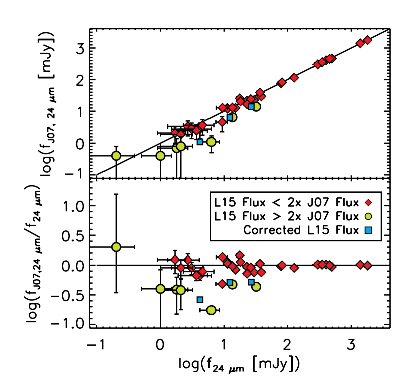
Figure 1: Top: J07 and T10 24 µm fluxes vs. fluxes obtained in this paper (with new 3.6 µm-based apertures) for galaxies in common. Higher fluxes ($\gtrsim 60$ mJy) fall close to the one-to-one line. The 7 galaxies for which we measure fluxes more than $2\times$ larger than the J07 fluxes have either larger apertures in our method or contaminating sources (indicated with green circles, while the corrected fluxes are marked with blue squares). We are using the values obtained with our 3.6 µm-defined Kron apertures for the remainder of the work. Bottom: Residuals for top panel plot.

In quiescent galaxies, populations of evolved stars contribute measurable emission in the UV (from horizontal branch stars) and at 24 µm (from asymptotic giant branch stars; Kaviraj et al. 2007). This can be seen in Figure 2 where we plot the level of $uvw2$ versus 24 µm fluxes as fractions of the 3.6 µm flux. Galaxies found in the region above and to the right of the dotted lines have both UV and MIR emission dominated by star formation, and we see that most of the MIR-active (actively star-forming) galaxies lie in this region. Objects in the lower right region are possibly reddened (and thus depressed UV flux) whereas the UV and MIR light of objects in the lower left region is dominated by old stellar populations. To account for this, we correct the $uvw2$ and 24 µm fluxes for contamination by emission from old stellar populations before converting them to star formation rates, following the method of Ford et al. (2013). The authors used the following equations to perform this correction

$$I_{\rm{FUV,SF}}=I_{\rm{FUV}}-\alpha_{\rm{FUV}}I_{\rm{3.6}}$$ (2)

$$I_{\rm{24,SF}}=I_{\rm{24}}-\alpha_{\rm{24}}I_{\rm{3.6}}$$ (3)

where $I$ represents intensity. Additionally, $\alpha_{\rm{FUV}}=I_{\rm{FUV}}/I_{\rm{3.6}}=0.003$ and $\alpha_{\rm{24}}=I_{\rm{24}}/I_{\rm{3.6}}=0.1$. These values were obtained by Leroy et al. (2008) by looking at the ratio of fluxes in elliptical galaxies. The $uvw2$ filter is more similar to GALEX NUV (used by Leroy et al. 2008) than it is to FUV, and so we examine whether the $\alpha_{\rm{FUV}}$ parameter may have a systematic offset. In Smith et al. (2012, see their Fig. 1), we see that the GALEX $FUV-NUV$ colour distribution (where FUV and NUV are in magnitudes) of massive quiescent galaxies with $r$-band luminosities of $\gtrsim 10^{9.5}$ $\mathrm{L_{r}}/\mathrm{L_{\odot}}$ is flat (with significant scatter). Since most galaxies in our sample fall within that range, we choose to set $\alpha_{uvw2}=\alpha_{\rm{FUV}}$.

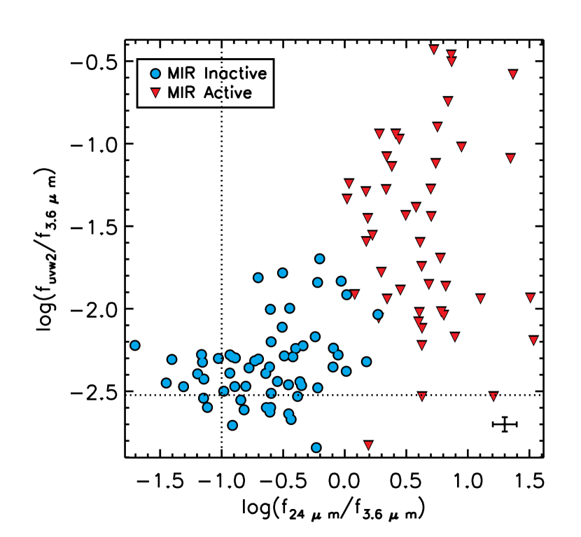
Figure 2: The $uvw2$ versus 24 µm emission with both axes normalized to the 3.6 µm fluxes. The data points are colour-coded according to their MIR colours. MIR-inactive galaxies are quiescent, and MIR-active galaxies are actively star-forming. The dashed horizontal line corresponds to UV-correction factor, $\alpha_{uvw2}=0.003$ and the dashed vertical line corresponds to MIR-correction factor, $\alpha_{24}=0.1$. The region above and to the right of the dotted lines contains galaxies whose UV and MIR light is dominated by star formation. Galaxies outside of this region likely have their UV and/or MIR light dominated by emission from old stars.

2.6 Stellar Masses

Stellar masses were calculated from the IRAC 3.6 and 4.5 µm photometry according to the prescription of Eskew et al. (2012):

$$M_{*}=10^{5.65}F_{3.6}^{2.85}F_{4.5}^{-1.85}\left(\frac{D}{0.05}\right)^{2}(\mathrm{M_{\odot}})$$ (4)

where $D$ is the luminosity distance of each CG given in Table 1. In brief, Eskew et al. (2012) used extinction and star formation history maps of the Large Magellanic Cloud to calculate its stellar mass, and calibrate the 3.6 and 4.5 µm fluxes for the purpose of stellar mass measurements. We compare this method to that of Bell et al. (2003) and McGaugh & Schombert (2015), and present the results in Figure 3. Bell et al. (2003) use a sample of galaxies from the Two Micron All Sky Survey and the Sloan Digital Sky Survey to derive a luminosity and stellar mass function, based on $K$-band luminosities. We compare the stellar masses calculated according to Eskew et al. (2012) with the stellar masses of Tzanavaris et al. (2010), which are calculated using the relation of bell03), and see that there is good agreement between these two methods, with some slight scatter about the one-to-one line. McGaugh & Schombert (2015) use a sample of 26 galaxies to constrain the slope of the Baryonic Tully-Fisher relation and use this to derive $K$-band and 3.6 µm mass-to-light ratios that are independent of the initial mass function. Their sample goes down to a mass of 3 $\times$ 10⁷ M_⊙. We have used their 3.6 µm mass-to-light ratio to calculate stellar masses and compare to our values. Our stellar masses agree well with those calculated according to McGaugh & Schombert (2015). We find that all of our stellar masses are in very good agreement with those derived using the method of McGaugh & Schombert (2015) and Bell et al. (2003), and proceed with the values we calculated with the relation of Eskew et al. (2012). Note that PAH emission from starbursting dwarfs (e.g., HCG 31F) may cause the masses to be overestimated in these types of galaxies (Desjardins, 2015).

Figure 3: Log of the stellar masses derived following Bell et al. (2003) and McGaugh & Schombert (2015) vs. the log of the stellar masses derived from the relation of Eskew et al. (2012) used in this paper. The one-to-one line is overplotted. The stellar masses derived from the relation of McGaugh & Schombert (2015) are very well correlated to the stellar masses derived in this work and they fall below the one-to-one line by a median of about 20 per cent. The stellar masses derived from the method of Bell et al. (2003) are also well correlated to the stellar masses derived in this work, and show only slight scatter about the one-to-one line.

2.7 Star Formation Rates

Active star formation in galaxies can be traced directly by studying UV emission from massive O and B stars and indirectly by studying IR emission, from dust heated by the light from these stars. UV-based SFRs must be corrected for intrinsic extinction in order to avoid underestimating their true values (Kennicutt, 1998; Salim et al., 2007), whereas IR-based values of SFR assume that most of the UV emission is absorbed and re-emitted in the IR (Calzetti et al., 2007; Rieke et al., 2009). Therefore, a complete picture of the star formation in our sample of compact groups can be obtained by measuring the dust-obscured component of the SFR from the MIR emission, and the unobscured component of the SFR from the UV light. In this section, we are following the methodology of T10, and briefly describe it here.

The $uvw2$ filter has an effective wavelength of 2030 Å, which is approximately in the middle of the UV 1500–2800 Å range. This therefore provides a “mean” estimate of the UV emission properties of CGs in our sample. Hence, for this study, the $uvw2$ filter luminosities were used to determine the UV contribution to SFR_TOTAL. The relation between luminosity and SFR_UV is given by equation 5 (Kennicutt, 1998). Equation 6 (Rieke et al., 2009) uses the calorimeter assumption (e.g., completely obscured star formation) calibrated to 24µm luminosities; we use this relation to measure the IR component of SFR_TOTAL. Finally, the total SFR is measured by simply adding the two components together, as in equation 7.

$${\rm SFR}_{uvw2}(M_{\odot}\,{\rm yr^{-1}})\equiv 9.5\times 10^{-44}\nu L_{\nu,uvw2}\ ({\rm erg\,s^{-1}})$$ (5)

$${\rm SFR}_{24\mu m}(M_{\odot}\,{\rm yr^{-1}})\equiv 2.03\times 10^{-43}\nu L_{\nu,24\mu m}\ ({\rm erg\,s^{-1}})$$ (6)

$${\rm SFR}_{TOTAL}\equiv{\rm SFR}_{uvw2}+{\rm SFR}_{24\mu m}$$ (7)

Our sample includes several early-type galaxies. Davis et al. (2014) use the results of Hao et al. (2011) to combine 22 µm WISE data and GALEX FUV data to derive SFRs for early-type galaxies in the ATLAS^3D sample. We note that the Hao et al. (2011) near-UV+25 µm calibration (SFR [M_⊙ yr^-1] $=1.1\times 10^{-43}L_{\rm 2000{\textup{\AA}}}$ [erg s^-1] $+2.4\times 10^{-43}L_{25\mu m}$ [erg s^-1]) corresponds well to our version. Although Davis et al. (2014) use FUV instead, as was discussed in section 2.5, the GALEX $NUV-FUV$ distribution for galaxies with r-band luminosities $\gtrsim$ 10^9.5 $\mathrm{L_{r}}/\mathrm{L_{\odot}}$ is flat. Since most CG galaxies in our sample satisfy this condition, we do not expect that the method of Davis et al. (2014) for calculating SFRs will yield results that are substantially different from the ones presented in this work.

Specific star formation rate (SSFR) values were also calculated in order to probe the star formation history of the galaxies in our sample, in addition to studying current star formation. SSFR is given by:

$${\rm SSFR}\equiv\frac{{\rm SFR}}{M_{*}}$$ (8)

where the stellar mass values were obtained from equation 4.

2.8 Comparison to Bitsakis et al. (2014)

For the 93 galaxies that we have in common, we have compared our SFR, stellar mass, and SSFR values to those of Bitsakis et al. (2014). We find that the SFR and stellar mass results derived in this work are systematically higher than those of Bitsakis et al. (2014)(median of 132 per cent and 2 per cent higher respectively). The SSFRs are observed to be scattered about the one-to-one line. In order to understand the offsets, we compare photometry, and examine the methodologies and assumptions of both studies.

2.8.1 Photometry

There are differences in photometry that could partially account for the systematic discrepancies. Bitsakis et al. (2014) used 3.6 µm data to define apertures, much like we did. These apertures were used across all of their data, however none of their data was convolved to the resolution of the largest beam (of Herschel SPIRE 500 µm). Instead, if the beam size was larger than the 3.6 µm-defined aperture they used the beam size to extract the photometry (T. Bitsakis, 2015, priv. comm.). Further, they also use slightly different luminosity distances from those used in our work. To mitigate this effect, we have compared our measured UV and MIR fluxes directly to those of Bitsakis et al. (2011). The IR fluxes are in good agreement, while the UV fluxes in Figure 4 show some scatter about the one-to-one line. We define offsets as the fractional difference between the linear fluxes we derive ($f_{\rm L15}$) and the fluxes of Bitsakis et al. (2011) ($f_{\rm B11}$))

$$\frac{f_{\rm L15}-f_{\rm B11}}{f_{\rm L15}}$$ (9)

The UV flux offsets have a mean of $-51$ per cent, a median value of $-21$ per cent and a standard deviation of 150 per cent, while the IR flux offsets have a mean, median and standard deviation of $-2$ per cent, 5 per cent, and 72 per cent respectively. Thus, the GALEX NUV fluxes of Bitsakis et al. (2011) are in general higher than the UV fluxes we derive and this can be seen from Figure 4, while the IR fluxes are in much better agreement.

Kaviraj et al. (2007) showed that UV fluxes can become contaminated by post-starburst stellar populations. While this possibility cannot be excluded, we note that there are no extreme UV outliers in the UV vs. MIR luminosity plots in Figure 6. It is thus unlikely that this is a major concern for our galaxies.

Emission from hot dust around AGN can contaminate the 24 µm data (Sanders et al., 1989); however Tzanavaris et al. (2014) showed that out of 37 HCG galaxies, only two are strong AGN while the remaining have X-ray nuclei consistent with low-luminosity AGN or a circumnuclear X-ray binary population. In addition, the MIR fluxes derived in this work agree well with those derived by Bitsakis et al. (2014), therefore it is unlikely that this might be the cause for the discrepancy between this work and the work of Bitsakis et al. (2014).

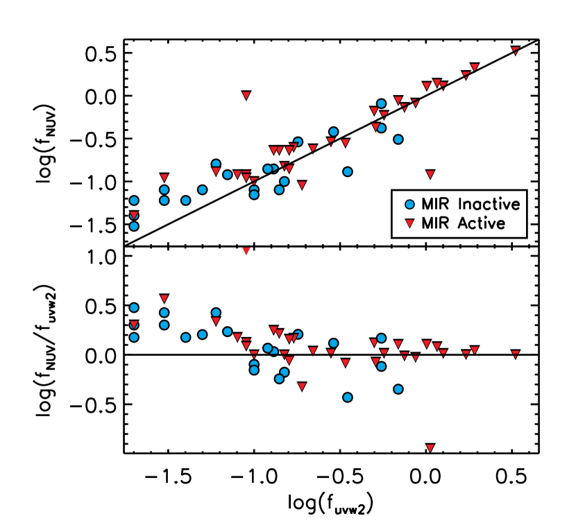
Figure 4: Top: GALEX NUV fluxes of Bitsakis et al. (2014) plotted against the Swift $uvw2$ fluxes of this work, separated according to MIR activity. In general, the NUV fluxes are higher than the $uvw2$ fluxes for fainter galaxies, however there does not seem to exist any relation to the MIR activity. Bottom: Residuals for the top panel.

2.8.2 Methodology

To assess the contribution of differences in methodology between this work and the work of Bitsakis et al. (2014), we use the NUV and 24 µm fluxes from Bitsakis et al. (2011) to derive SFRs using our methodology. By doing this, the SFRs calculated using our method and the photometry of Bitsakis et al. (2011) show a median increase of $\approx$90 per cent, relative to the SFRs reported in Bitsakis et al. (2014).

The greatest differences are seen at the low end of the SFR range of values (quiescent galaxies); our method estimates higher SFRs for quiescent galaxies than does the method of Bitsakis et al. (2014). It is important to note that galaxies which Bitsakis et al. (2014) find to be low star formation rate galaxies are also identified as such using our method. For example, Bitsakis et al. (2014) report a SFR of 0.01 $M_{\odot}$ yr^-1 for HCG 15C, while we find a SFR of 0.12 $M_{\odot}$ yr^-1. For more actively star forming galaxies, the increases in SFRs (our values versus theirs) are much smaller. This accounted for some of the systematic discrepancy. There is a remaining median difference of $\approx$43 per cent. We attribute the rest to differences in methodology, which we further discuss.

Bitsakis et al. (2014) use SED-fitting of the observed UV to sub-millimeter (152.8 nm to 500 µm) luminosities to estimate the star formation rates and stellar masses of individual galaxies. They use the MAGPHYS code (da Cunha et al., 2008) to interpret their SEDs and obtain these physical parameters. MAGPHYS is a stellar population synthesis model which uses the Galactic disk initial mass function (IMF) of Chabrier (2003). The version of MAGPHYS used by Bitsakis et al. (2014) employs the Bruzual & Charlot (2003) stellar-population synthesis models because the libraries of Charlot & Bruzual (2007) overestimate the importance of the thermally pulsing asymptotic giant branch (TP-AGB), and therefore inaccurately overpredict the near-IR luminosities in the stellar evolution models, leading to an underestimate of stellar masses (Zibetti et al., 2012).

In comparison, the calibrations of Kennicutt (1998) and Rieke et al. (2009) that we use to calculate SFRs assume a Salpeter IMF and do not depend on population synthesis models. The model of Eskew et al. (2012) we use to determine stellar masses also does not rely on population synthesis models. Rather, the authors performed star counts in the Large Magellanic Cloud with NIR data, and used this to calibrate a conversion between 3.6 and 4.5 µm fluxes, and stellar mass. This approach to determining stellar mass still has some dependence on the IMF and on stellar evolution models, however, it does not depend on the star formation history and therefore minimizes the effects of rare stages of stellar evolution such as the TP-AGB phase. Their model favours bottom-heavy IMFs such as that of Salpeter (1955), and disfavours bottom-light IMFs such as that of Chabrier (2003).

As an independent check, we have derived stellar masses using the 3.6 µm mass-to-light ratio of McGaugh & Schombert (2015) and have found that they correlate very well with the stellar masses we have derived using the relation of Eskew et al. (2012). The method of McGaugh & Schombert (2015) is independent of the IMF and the authors find a 3.6 µm mass-to-light ratio of 0.45 M_⊙/L_⊙, compared to 0.5 M_⊙/L_⊙ found by Eskew et al. (2012).

2.8.3 Conclusion

After performing this comparison, we are confident that we have ruled out any unknown systematics in our treatment that leads to the mostly small discrepancies with Bitsakis et al. (2011). The most important point to make however, is that despite the differences in derived values, our results are not affected qualitatively. The bimodality we observe in SSFRs remains intact regardless of what values we choose to use. Therefore, we now proceed with our analysis using our derived values.

3 Results and Discussion

3.1 UV Results

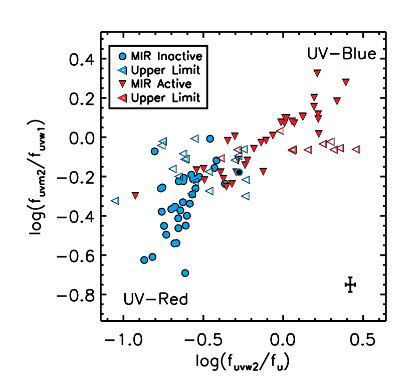
Figure 5: UV colour-space distribution, defined in terms of flux ratios, of 101 galaxies from our sample of 192 CG galaxies. The hollow data points are those which suffer from coincidence loss in the $u$ filter and are therefore upper limits (along the horizontal axis). MIR-active galaxies are found to be UV-blue, as expected if they are actively star-forming galaxies, while the MIR-inactive galaxies are found to generally be UV-red, consistent with being quiescent galaxies. The median error bars are presented in the bottom right corner.

In Figure 5, we have plotted the colour-space distribution of 101 galaxies for which we have data in all four UV filters. We do this to investigate whether the UV colours can independently tell us something about the status of star formation in the CG environment. We have indicated in red triangles galaxies which are MIR-active (i.e., actively star-forming) and indicated in blue circles galaxies which are MIR-inactive (i.e., quiescent) according to the criteria of Walker et al. (2012). The majority of MIR-active galaxies are also UV-blue, and the MIR-quiescent galaxies are UV-red as expected if ongoing star formation contributes UV-light from young, massive stars as well as dust and PAH emission. There is some overlap between these two populations in this particular colour-space without a gap or canyon; the distribution is continuous. The data (especially where there is no coincidence loss) are well correlated. The Spearman test supports this, returning a Spearman rank coefficient of 0.87 and a significance of $5.9\times 10^{-32}$, indicating a significant correlation between the two UV colours. If we remove the data that suffer from coincidence loss (the unfilled points), we find a Spearman Rank coefficient of 0.89 with a significance of $8.6\times 10^{-25}$.

We notice in this colour-space that there is a sort of plateau in $\log(F_{\rm uvm2}/F_{\rm uvw1})$ of 8 MIR-active galaxies: HCG 2A, HCG 2B, HCG 22C, HCG 31ACE, HCG 31G, RSCG 31B, RSCG 44C and RSCG 66A. These are all upper limits as they are saturated in the $u$ filter, and thus have only lower limits to their $F_{\rm u}$ values. Since the upper limits are in the x-axis, the true $\log(F_{\rm uvw2}/F_{u})$ values are to the left of the open data points. There is also one MIR-active galaxy which appears to be UV-red. This is the edge-on spiral galaxy HCG 37B, and therefore likely suffers from significant reddening in the UV.

3.2 MIR and UV Comparisons

We have plotted the $uvw2$ and 24 µm luminosities for individual galaxies in Figure 6 and have indicated the galaxies according to morphology (E/S0 or S/Irr) and according to the parent-group H i richness for each galaxy. The luminosities are mildly correlated (Spearman Rank coefficient of 0.58 with a significance of $1.9\times 10^{-11}$) but with considerable scatter that increases at $\sim$ 10⁴² erg s^-1. When coded by morphology, it becomes clear that E/S0 galaxies are typically less luminous at both UV and MIR wavelengths, even though they are also typically more massive. This is expected since we would expect to see more star formation in S/Irr galaxies. We also notice that the galaxies in our sample are generally more luminous in the UV rather than the MIR. This implies that there are not significant amounts of embedded star formation only detectable at 24 µm.

However, there is a population of galaxies which fall below the one-to-one line indicating that they have stronger MIR emission compared to the UV. The majority of these galaxies are S/Irr, and so they may have significant dust along the line of sight that depresses the UV emission relative to the MIR. From visual inspection of the Swift $u$ images, we find that of the 29 galaxies which fall to the right of the one-to-one line, 7 have E/S0 morphologies, 5 galaxies appear to be (near) face-on spirals, and approximately half (17) are high inclination (close to edge-on) spirals. None of the MIR-brighter E/S0 galaxies (HCGs 2B, 37E, 90B and RSCGs 4B, 4C, and 17C) are known AGN according to NED. Furthermore, most of the galaxies which fall below the one-to-one line reside in groups of intermediate H i gas-richness. This could be due to there not being a large number of H i-rich groups, and H  i-poor groups do not contain many spiral galaxies. The overall group type does not segregate galaxies in this parameter space, though we see a general trend that galaxies in H i-poor groups have lower UV and MIR luminosities, and correspond to E/S0 type galaxies. Galaxies in H i- rich groups generally have higher UV and MIR luminosities and correspond more to S/Irr galaxies. Galaxies in groups of intermediate H i-richness span the range of UV and MIR luminosities.

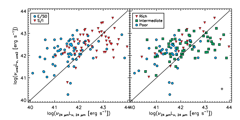
Figure 6: log($\nu_{uvw2}L_{\nu,uvw2}$) vs. log($\nu_{\rm 24\mu m}L_{\nu,24\mu m}$) for 114 CG galaxies. Left: Galaxy symbols indicate E/S0 (blue circles) and Sp/Irr (red triangles) morphologies. All CG galaxies are in general more luminous at UV wavelengths, than MIR. Right: Galaxy symbols indicate parent group H i type. Galaxies in gas-rich groups are indicated with squares, intermediate groups with circles, and poor groups with triangles. These parent group H i types are defined according to dynamical mass, as found in J07. Galaxies in H i-rich groups tend to be more luminous than those in H i-poor groups, while galaxies residing in groups of intermediate H i content span the range of luminosities. For reference, a one-to-one line is overplotted in both panels. Median error bars are presented in the bottom right corner of the right panel.

In Figure 7, we have plotted the distribution of $uvw2$ luminosities for the full sample of CGs which have available data in this filter, as well as subsamples based on the total H i content of the group. Using the definition of J07, gas richness is defined as: H i rich groups have $\log(M_{\rm HI})/\log(M_{\rm dyn})\geq 0.9$, H i intermediate groups have $0.9>\log(M_{\rm HI})/\log_{10}(M_{dyn})\geq 0.8$ and H I poor groups have $\log_{10}(M_{H~{}{\sc I}})/\log_{10}(M_{dyn})<0.8$. In contrast to what was found by T10 (see their Figure 10), with this larger sample, we see considerable overlap between the $uvw2$ luminosities of galaxies in the three levels of H i-richness. We have, however, performed a Mann Whitney U test (RS_TEST in IDL) on the three subsamples defined by H i group type and have found the following probabilities that the subsamples have the same median distribution: 0.221, 0.004 and 0.001, when comparing the galaxies in rich and intermediate groups, rich and poor groups, and intermediate and poor groups. Probabilities that are lower than the 0.05 significance level indicate that the two samples being tested do not have the same median distribution. This suggests that the H i-rich and intermediate groups share the same median distribution, while the H i-rich and poor, and H i-intermediate and poor groups are different. We also performed the two-sided Kolmogorov-Smirnov test (KS_2SAMP in Python) and found similar results. The $p$-values returned were 0.61, 0.04, and 0.01 when comparing H i-rich and intermediate groups, rich and poor, and intermediate and poor, respectively. The $p$-value for the H i-rich and intermediate groups is high, 61 per cent, and therefore we can consider these two distributions to be statistically consistent. The $p$-values for the H i-rich and poor, and intermediate and poor groups, are both less than 5 per cent so we can consider them to be statistically different. Rich, intermediate and poor groups seem to all have more galaxies at intermediate luminosities. Rich groups seem to have somewhat more UV-luminous galaxies than intermediate and poor groups, and poor groups seem to have somewhat UV-fainter galaxies than rich and intermediate. This is consistent with more cold gas present in rich groups enabling higher levels of star formation.

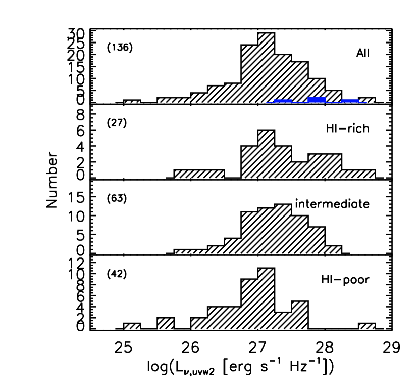
Figure 7: Histogram of the $uvw2$ monochromatic luminosities for the full sample of CGs. The distribution for the entire sample is shown, as well as subsamples defined by the group H i content. Data points HCG 71A, HCG 71B, HCG 71C and RSCG 66A have an undetermined H i group type and are therefore plotted in solid blue in the top panel. The number of galaxies in each panel is given in parentheses in its upper left corner.

3.3 SFR and SSFR Results

Our SFR_UV, SFR_IR and SSFR values, along with the UV and IR luminosities are given in Table 6. This Table also includes stellar masses (calculated with equation 4), and $\alpha_{\rm IRAC}$ values of each galaxy. The $\alpha_{\rm IRAC}$ parameter was defined by Gallagher et al. (2008) as the spectral index of the power-law fit to the 4.5, 5.6, and 8.0 µm luminosity densities, $l_{\nu}\propto\nu^{\alpha_{\rm IRAC}}$. MIR-active galaxies (with red MIR spectral energy distributions from warm dust and PAH emission) have $\alpha_{\rm IRAC}\leq 0$, whereas MIR-quiescent galaxies (with blue MIR SEDs consistent with stellar photospheric emission) have $\alpha_{\rm IRAC}>0$. The $\alpha_{\rm IRAC}$ values presented in Table 6 were measured by fitting a power-law to the Walker et al. (2012) IRAC photometry.

Table 6: UV and IR Properties of HCG and RSCG Galaxies. The full table is available online.

CG	Galaxy	$\log$ Lν (erg s-1 Hz-1)					log M∗	$\alpha_{\rm IRAC}$a	SFRuvw2	SFR24μm	SSFR
ID	Morphology	$uvw2$	$uvm2$	$uvw1$	$u$	24 $\mu$m	(M⊙)		(M⊙ yr-1)	(M⊙ yr-1)	(10-11 yr-1)
HCG 2A	S	28.05	28.27	28.24	28.41	29.70	10.35	-2.68	2.523	1.335	17.230
HCG 2B	S	27.62	27.88	27.83	28.06	30.13	10.22	-3.63	0.957	3.645	27.778
HCG 2C	S	27.45	27.71	27.66	27.95	28.94	10.15	-2.38	0.659	0.232	6.322
HCG 4A	S	$\cdots$	28.63	28.68	28.92	30.78	11.18	-3.47	$\cdots$	16.348	$\cdots$
HCG 4B	S	$\cdots$	27.77	27.83	27.13	29.27	10.40	-2.64	$\cdots$	0.496	$\cdots$
HCG 4D	E	$\cdots$	27.58	27.66	27.92	29.65	10.33	-3.33	$\cdots$	1.190	$\cdots$
HCG 7A	S	27.49	27.51	27.77	28.25	30.03	10.96	-2.37	0.435	2.894	3.631
HCG 7C	S	27.93	27.96	28.03	28.34	29.45	10.65	-2.45	1.203	0.758	4.352
HCG 7D	S0	27.35	27.40	27.46	27.83	28.58	10.14	-2.41	0.352	0.103	3.043
aGallagher et al. (2008) defines the $\alpha_{\mathrm{IRAC}}$ parameter. Desjardins et al. (2014) describes the method of SED fitting from which the values presented here were calculated.

Figure 8 shows a histogram of the SFRs separated into two subsamples: MIR-active and MIR-quiescent defined according to the $\alpha_{\rm IRAC}$ values. Both the original sample of CGs studied by T10 and the sample of 46 CGs studied in this project show a continuous distribution of SFRs (Fig. 12 in T10 and our Fig. 8). The original sample from T10 shows a flatter distribution, whereas the expanded sample is more peaked at around log(SFR) $=$ 0, indicating that the most common SFR value in CGs might be $\approx$1 $M_{\odot}$ yr^-1. Despite the significant overlap between MIR-active and MIR-inactive galaxies, we do see that quiescent galaxies ($\alpha_{\rm IRAC}>0$) are less star-forming and active galaxies ($\alpha_{\rm IRAC}\leq 0$) have higher star formation rates on average. The total distribution has a mean log(SFR) and standard deviation of $-0.29\pm 0.72$ $\mathrm{M}_{\odot}~{}\mathrm{yr}^{-1}$. The population of galaxies with $\alpha_{\rm IRAC}>0$ has a mean log(SFR) and standard deviation of $-0.66\pm 0.55$ $\mathrm{M}_{\odot}\mathrm{yr}^{-1}$ whereas the population of galaxies with $\alpha_{\rm IRAC}\leq 0$ has $0.04\pm 0.69$ $\mathrm{M}_{\odot}\mathrm{yr}^{-1}$.

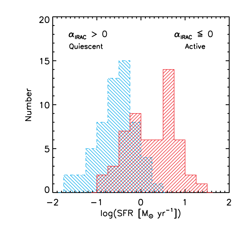
Figure 8: SFR distribution for 114 CG galaxies. The sample is separated into two subsamples; MIR-active ($\alpha_{\rm IRAC}\leq 0$; red hashed histogram) and MIR-quiescent ($\alpha_{\rm IRAC}>0$; blue hashed histogram). Though the medians of the two populations are offset, the distributions have significant overlap, and the total distribution of SFRs is continuous.

The same separation according to $\alpha_{\mathrm{IRAC}}$ does not yield a continuous distribution for SSFRs as we can see in Figure 9. In the left panel we show the distribution of SSFR values that are not corrected for old stellar populations, whereas the right panel shows the corrected SSFR values. Even before applying the correction for contamination by old stellar populations, we see that the distribution of SSFRs is bimodal. Applying the correction only makes the dip more pronounced. The dip appears at $0.2\leq\textrm{log}(\textrm{SSFR}[10^{-11}\mathrm{yr}^{-1}])\leq 0.4$ and is indicated in both panels with dotted lines. This dip region is defined as half the median value of the histogram. We performed the Hartigan Dip Test using the R package diptest, to check the statistical significance of this bimodality. The Hartigan Dip Test (Hartigan & Hartigan, 1985) measures a distribution’s departure from unimodality by minimizing the maximum difference between an empirical distribution and a unimodal distribution. The resulting dip statistic (D_n) indicates that a distribution is significantly bimodal if it is $\leq 0.05$ and only marginally bimodal if it is between $0.05$ and $0.1$. After performing this test, the resulting dip statistic, D_n = 0.02, indicates that the distribution is significantly bimodal. Thus, the bimodality that was previously found by T10 is still present even after significantly increasing the sample size, suggesting a fast transition from active star formation to quiescence in CG galaxies. The mean and standard deviation of the total log(SSFR) distribution is $0.20\pm 0.65$ $10^{-11}\mathrm{yr}^{-1}$. For the population of quiescent galaxies ($\alpha_{\rm IRAC}>0$), they are $-0.23\pm 0.42$ $10^{-11}\mathrm{yr}^{-1}$, while for the population of actively star-forming galaxies ($\alpha_{\rm IRAC}\leq 0$), they are $0.67\pm 0.51$ $10^{-11}\mathrm{yr}^{-1}$.

Since the most massive galaxies would have formed earlier in time, one might expect that they should have lower SFRs. Due to their high stellar masses, they will also have lower values of SSFR. Correspondingly, we would expect galaxies with higher SFRs and SSFRs to be lower mass galaxies because they have (consistent with cosmic downsizing) both larger reservoirs of gas for star formation and lower stellar masses.

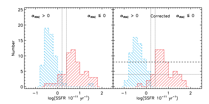
Figure 9: Distribution of SSFRs for 117 CG galaxies. Left: Distribution of SSFRs uncorrected for old stellar populations. Right: Distribution of SSFRs corrected for emission from old stellar populations. The values in both panels are separated into two different populations, according to their $\alpha_{\rm{IRAC}}$ values. Both panels show a clear bimodality in the values of SSFRs. The values of SSFR show even less overlap according to $\alpha_{\rm{IRAC}}$ values when they are corrected for emission by old stellar populations. The vertical lines mark the “dip” in the distribution of the total population of SSFRs, defined as half the median value of the histogram, where the dashed horizontal line indicates the median, and the dotted horizontal line marks the half median value.

Looking at Figure 10, we notice that the SSFR values correlate much better with H i-gas content of the group than did the $uvw2$ luminosities. Rich groups tend to have higher SSFRs, groups of intermediate H i-richness cover a broad range of SSFR values, and H i-poor groups tend to have lower SSFRs. This is consistent with the results from T10 (as shown in their Fig. 13).

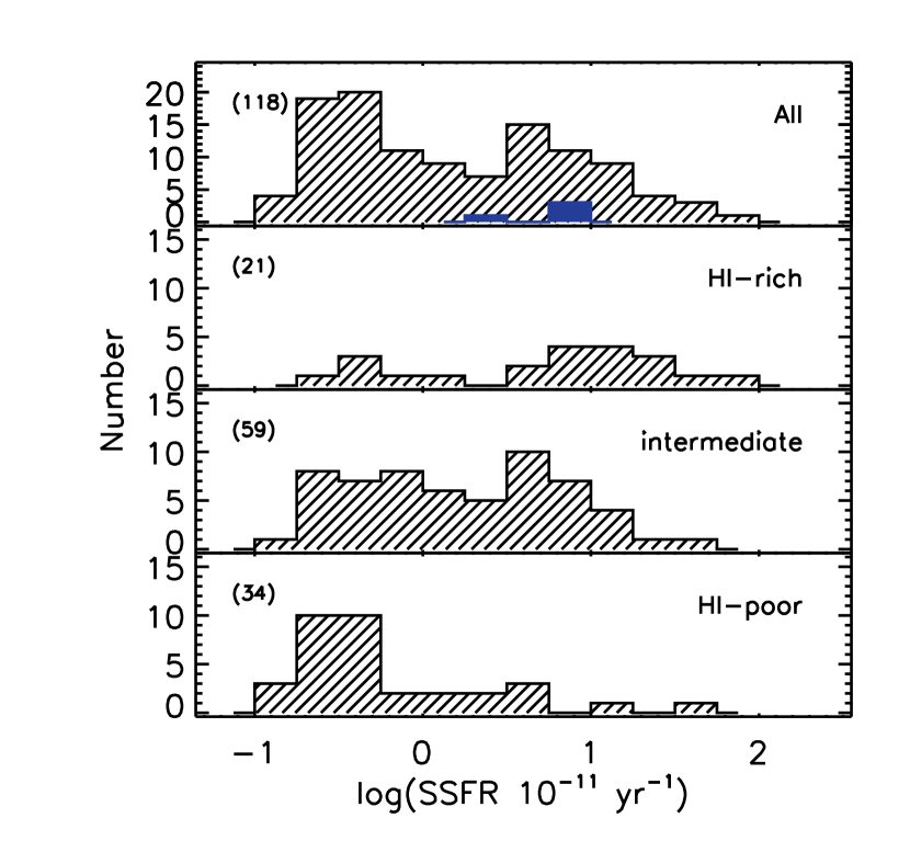
Figure 10: SSFR distribution for CG galaxies. The top panel shows the total distribution. The H i group type for HCG 71A, HCG 71B, HCG 71C and RSCG 66A are undetermined and plotted in dark blue. The next three panels show subsamples determined by the group H i content. The number of galaxies in each panel is indicated in the left corners.

In Figure 11, we have plotted the MIR activity index, $\alpha_{\rm IRAC}$ versus SSFR. The plotting symbols indicate the parent-group H i richness. As also found by T10, it is clear from the plot that quiescent galaxies ($\alpha_{\rm IRAC}>0$) have lower SSFRs and they mostly reside in gas-poor or intermediate groups. We can also see that actively star-forming galaxies ($\alpha_{\rm IRAC}\leq 0$) also have higher SSFRs and reside mostly in gas-rich or intermediate groups. We have indicated in dashed lines the region where we see the dip (determined from the histogram in the right panel of Fig. 9). For comparison, we include vertical bold lines to indicate the gap region that was previously observed by T10. The horizontal bold lines indicate gap region in $\alpha_{\mathrm{IRAC}}$ values. Due to larger numbers, it is perhaps not surprising that the earlier SSFR gap (T10) is now observed as a dip, which is shown to be statistically significant.

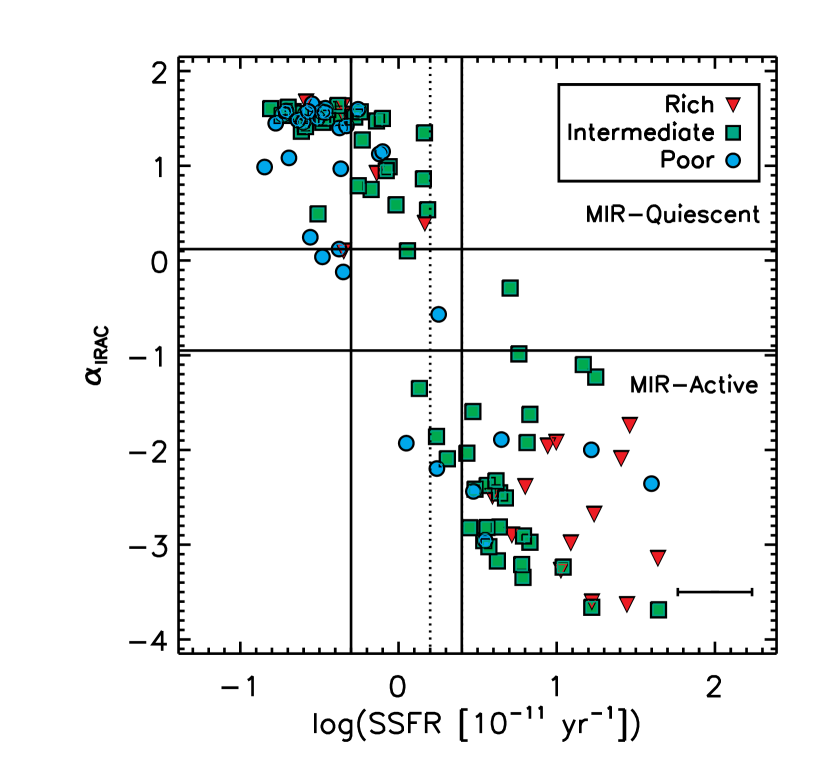
Figure 11: MIR activity index, $\alpha_{\rm IRAC}$ vs. $\log(SSFR)$ for 114 galaxies (corrected for emission from old stellar populations). The different plotting symbols indicate different parent-group gas richness. The bold lines represent the SSFR and $\alpha_{\rm IRAC}$ gaps observed in T10. The dashed lines show where we see the dip in SSFRs with the expanded sample of CGs.

In Figure 12, we plot the total group SFRs versus the H i content of each group and find that groups span the full range of SFR values regardless of their group type. This again shows that the quantity of interest is the SSFR of each group, not its SFR. We also plot the total group SSFRs versus the H i content of each group in Figure 13. The left panel contains H i content defined in terms of stellar mass, while the right panel contains H i content defined according to dynamical mass (J07). When we define the H i content types according to stellar mass, there is a clear trend of increasing values of SSFR with increasing richness in parent-group H i content, supporting the idea that SSFR tracks gas depletion (T10).

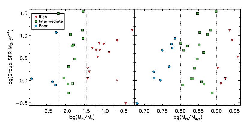
Figure 12: Total group SFR vs. $\log M_{H~{}{\sc I}}/\log M_{*}$ for every galaxy in our sample. The symbols indicate parent-group H i richness. We can see that the groups span the full range of SFR values regardless of their parent-group type.

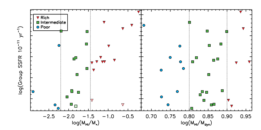
Figure 13: Total group SSFR vs. $\log M_{H~{}{\sc I}}/\log M_{dyn}$ for every group in our sample. The symbols indicate parent-group H i richness. We can see that the trend remains for H i rich groups to have higher values of SSFR, as in T10.

Finally, we plot in Figure 14 the $\log(F_{\rm uvw2}/F_{\rm u})$ flux ratio versus SFR and SSFR; symbols indicate MIR-active and MIR-inactive galaxies. When the UV flux ratio is plotted versus SFR, there is no strong correlation. However, when we plot this UV flux ratio against SSFR, a strong trend is evident. In this parameter space, two populations are clearly shown: MIR-active galaxies have higher SSFRs and tend to be UV-blue while MIR-inactive galaxies tend to be UV-red with lower values of SSFR. There is little overlap between the two populations. A few galaxies are discrepant: HCG 48C, HCG 37B and HCG 92C (a strong X-ray AGN, Tzanavaris et al. 2014) are MIR-active but also UV-red (lower part of plot). All three are spiral galaxies, but only HCG 48C and HCG 37B are edge-on. Therefore, the UV-flux ratio is likely reflecting intrinsic extinction in HCG 48C and 37B. The X-ray AGN HCG 92C is a Seyfert 2 galaxy, and so while the direct view of the UV AGN continuum is blocked, the AGN likely dominates the MIR emission.

We find 8 galaxies here as well which do not follow the general trend of the data. These galaxies are all MIR-active, but have lower UV flux ratios for their SSFRs. These galaxies are HCG 16D, HCG 40D, HCG 56B, HCG 56D, HCG 59A, HCG 71B, RSCG 4A and RSCG 4C.

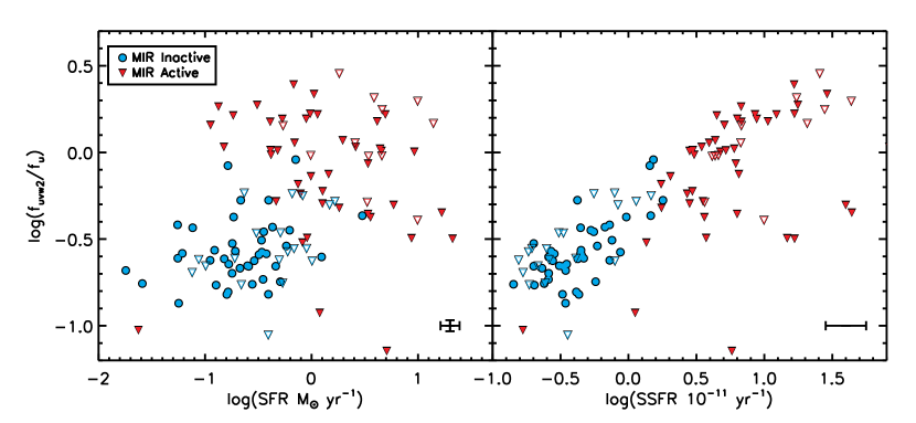
Figure 14: The $f_{uvw2}/f_{u}$ UV flux ratio has been plotted versus SFR (left panel) and SSFR (right panel) for the 115 galaxies for which all the data are available. The galaxies are colour-coded as MIR-quiescent (blue circles) and MIR-active galaxies (red triangles). While the UV-flux ratio shows a scatter plot vs. SFR, there is a significant trend whereby blue UV flux ratios correlate with increassing SSFRs. The combination of MIR-colour, UV-flux ratio, and SSFR measurements clearly separate the CG galaxy population into active and quiescent galaxies. Median error bars are shown in the bottom right corners of each panel.

3.3.1 Star-Forming “Main Sequence”

It has now been established that over the past 10 Gyr a correlation exists between SFR and $M_{\ast}$ for star-forming galaxies (Noeske et al., 2007; Elbaz et al., 2007; Daddi et al., 2007). Wuyts et al. (2011) studied large sample of more than 800,000 galaxies at different redshifts, confirming the correlation, albeit with a zero point that increases with redshift. We take our SFR and stellar mass measurements, and plot our sample of CGs in this parameter space, together with the best-fit results of Chang et al. (2015), to investigate how they compare to non-CG galaxies. Chang et al. (2015) adopt a mass limit, such that all galaxies in their sample have significant WISE 12 µm emission. Their galaxies all have redshift $<0.6$, with the majority having redshifts $<0.2$. We include all of our CG galaxies regardless of mass, and show the main sequence line, defined as the median values of 0.2 M_⊙ wide stellar mass bins ($\pm 1\sigma$) from Figure 11 of Chang et al. (2015) as a comparison to our sample. This comparison is illustrated in Figure 15, with galaxies separated according to MIR activity. This compares well to the results of Chang et al. (2015) as all CGs plotted in Figure 15 fall within their range of SFRs from $-3<\mathrm{log(SFR[M_{\odot}yr^{-1}])}<1$. Furthermore, we see that MIR inactive galaxies all fall below the $-1\sigma$ limit of the main sequence line. The MIR active galaxies however follow the main sequence line, with most galaxies falling within the $\pm 1\sigma$ limit. Of the 48 MIR-active galaxies plotted in this figure, 26 lie above the main sequence line.

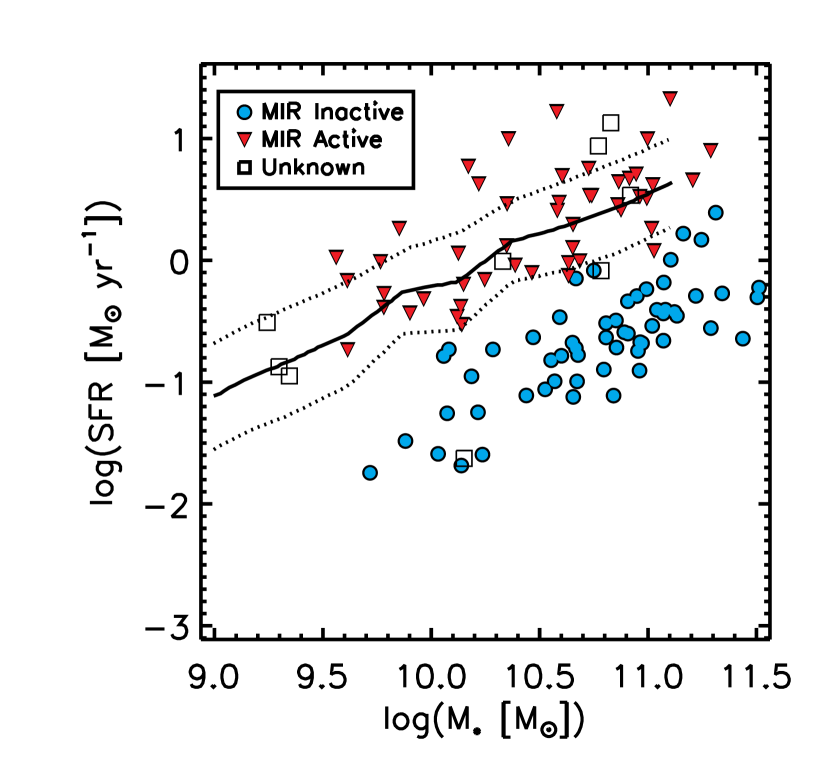
Figure 15: Plot of log(SFR) vs. log($M_{\ast}$). The solid black line is the median main sequence line from Chang et al. (2015), while the dotted orange lines represent the 1$\sigma$ limits. We plot the 118 CG galaxies for which we have SFR and M_∗ measurements. We separate the 118 CG galaxies according to their MIR activity and find that all MIR inactive galaxies fall below the $-1\sigma$ limit of the main sequence line, while the MIR active galaxies are generally within $\pm 1\sigma$ of the line. In cases where we do not have MIR activity information, we plot the data point as a black box. Based on their locations within this parameter space, the majority of these galaxies are likely to be MIR-active.

3.4 UV-Optical Results

Figure 16 is a UV-optical colour-magnitude plot. To be consistent with earlier GALEX work, we use data from the Swift $uvm2$ filter which is most similar to the GALEX NUV band. The bottom portion of Figure 16 is the region of star formating galaxies and these galaxies are accordingly MIR-active/UV-blue, the top portion represents the red sequence where passive or reddened galaxies reside and are accordingly MIR-quiescent/UV-red.

Figure 12 of Wyder et al. (2007) shows the volume density of galaxies as a function of $NUV-r$ for 0.5 mag wide bins. They note an underpopulation of galaxies in the region $3<NUV-r<5$ mag and refer to this as the “green valley”. We mark this region with horizontal dashed lines in Figure 16. The black data point in our Figure 16 is the galaxy HCG 37E, a MIR canyon galaxy, as defined in Walker et al. (2012) and just falls in this region of the UV-optical CMD. Otherwise there is no evidence for a green valley in this figure. This region is well populated with galaxies. However, we have not corrected our UV-optical colours for intrinsic extinction.

Comparing Figure 16 to Figure 14, we see that the UV-only colours are much cleaner than the UV-optical colour in separating galaxies according to MIR activity. The UV-only colour may be better at discriminating between low and high SSFRs because the UV-colour is sensitive to SSFRs as seen in Figure 14. However, in addition to this, the $uvw2$ and $u$ filters have a much narrower wavelength separation than do $uvm2$ and $r$. As long as there is no bump at around 2200 Å in the extinction curve (Stecher, 1969), the UV-only colour should be less susceptible to extinction.

We separate the data in Figure 16 according to the MIR activity of each galaxy. We also scale the data point symbols according to SSFR. The data are separated in bins of width equal to 0.4 $10^{-11}\textrm{yr}^{-1}$. The MIR-inactive galaxies all have lower SSFR values and all the MIR-active galaxies have higher SSFR values, as we would expect. It shows however, that the galaxies in the UV-optical green valley region, which are a mixture of MIR-active and MIR-inactive galaxies, all have intermediate SSFR values.

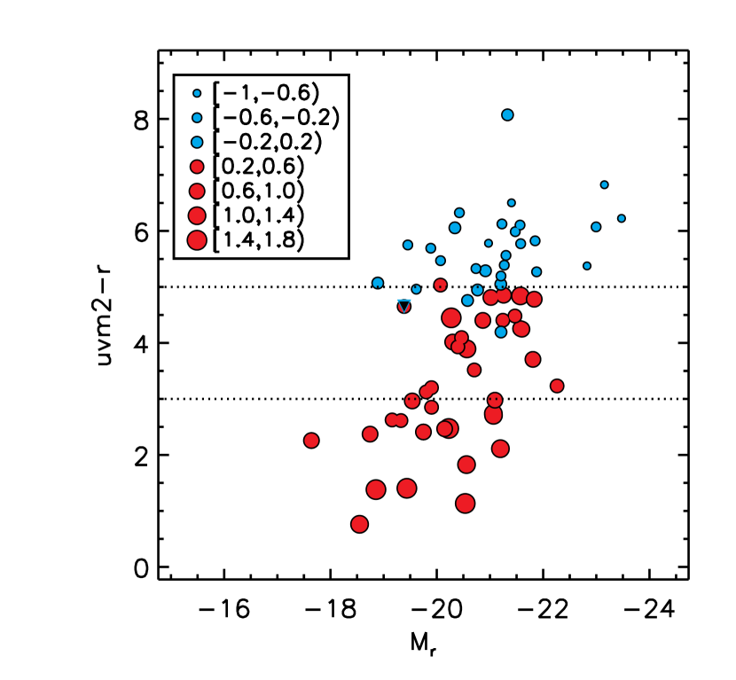
Figure 16: UV-optical colour-magnitude diagram for 69 galaxies in our sample. The number of data points in this figure is limited to galaxies for which we were able to determine SSFRs. The symbol sizes refer to bins of SSFRs with increasing symbol size corresponding to increasing SSFRs, as indicated in the legend. The bins have width of 0.4 10${}^{-11}\mathrm{M_{\odot}}$. We see that all galaxies along the red sequence ($uvm2-r>5$) have lower values of SSFR. The region of the blue cloud ($uvm2-r<3$) contains galaxies that have higher SSFRs. The green valley is populated by galaxies of intermediate SSFR levels. No corrections have been made for internal extinction.

Figure 17 plots the $uvm2-r$ colour vs the SFRs and the SSFRs. When we plot the $uvm2-r$ colour against the SFRs, there appears to be no correlation. However, the data is separated cleanly into two “clouds” delineated by the MIR colours. When we plot this colour against the SSFRs, we see that the data are highly correlated. This is not surprising since $uvm2$ is dominated by massive, short-lived stars, thus it traces SFR. On the other hand, $r$ traces stellar mass since it is sensitive to emission from older, longer-lived stars (Wyder et al., 2007; Martin et al., 2007; Thilker et al., 2010). We notice in the top right panel that there appears to be a separate little cloud of MIR-active galaxies at around $4\leq\mathrm{uvm2-r}\leq 5$ mag. These galaxies are HCG 7A, HCG 38A, HCG 38B, HCG 47C, HCG 56B, HCG 56D, HCG 59A, HCG 61A, HCG 71B, HCG 100A, and RSCG 4A. The scatter observed in these MIR-active galaxies is likely related to extinction.

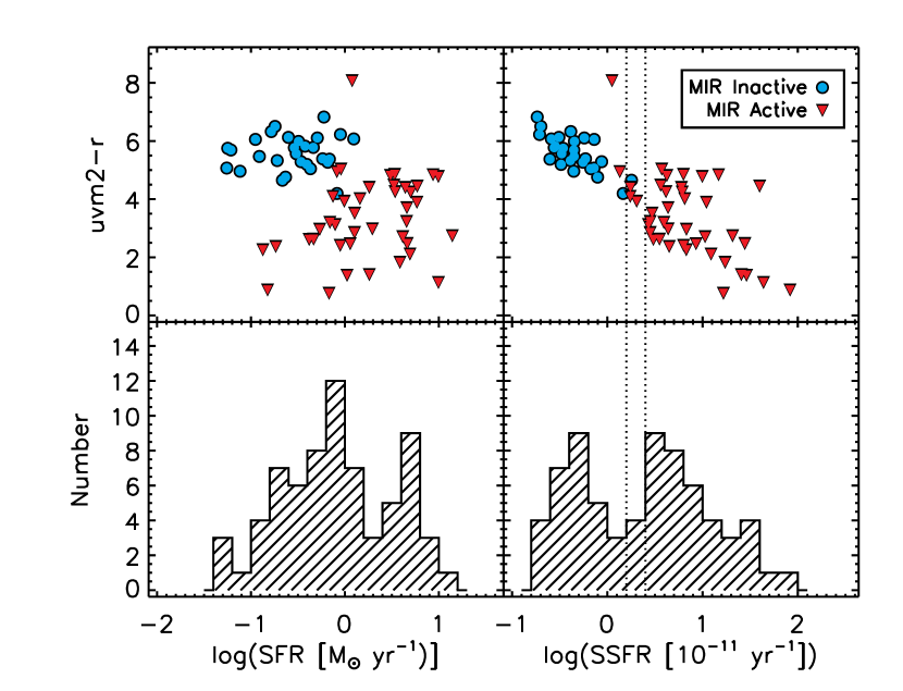
Figure 17: UV-optical colour vs. SSFR and SFR for the 69 galaxies for which we had available data. Top left: We plot the $uvm2-r$ colour vs. SFR and see that the data are scattered. We colour code the points according to MIR activity. We see that MIR active galaxies are generally more star forming and have bluer $uvm2-r$ colours. MIR inactive galaxies are less star forming and have redder $uvm2-r$ colours. Top right: We plot the $uvm2-r$ colour vs SSFR and find a much stronger correlation. Bottom left: Distribution of SFR values. Bottom right: Distribution of SSFRs. We use dotted lines again to indicate the dip region in SSFR values.

4 Summary and Conclusion

We have presented Swift UV ($uvw2$, $uvm2$, $uvw1$ and $u$) and Spitzer MIR (3.6 $\micron$, 4.5 $\micron$ and 24 $\micron$) photometry for 136, 130, 141, 146 and 169, 169, 154, CG galaxies respectively. We have combined the UV and MIR photometry to obtain star formation rates, stellar masses, and specific star formation rates for 118, 169 and 118 galaxies, respectively.

Including corrections for the contribution to the UV and MIR emission from old stellar populations. Compared to the earlier work of T10, the sample size in this paper represents an increase by a factor of about 4.

The main results of this paper are summarized here.

• We have confirmed the correlation between L_ν,uvw2 and L_ν,24μm (Figure 6) and shown that E/S0 galaxies are typically less luminous at UV and MIR wavelengths than S/Irr galaxies. CG galaxies are however generally more luminous at UV wavelengths than MIR, implying that there is not much embedded star formation in this population. Galaxies in H i-rich groups are generally more luminous at UV and MIR wavelengths than those in H i-poor groups, while galaxies in groups of intermediate H i gas richness span the range of UV and MIR luminosities.

• The UV $uvw2/u$ and $uvm2/uvw1$ flux ratios confirm our expectation that the MIR-active and UV-blue colours consistently trace young stellar populations. No gap or canyon is observed in this parameter space.

• As seen by T10, the SFR distribution is continuous though more peaked than seen previously with the most likely SFR in compact group galaxies of $\sim 1\rm{M_{\odot}yr^{-1}}$. Figure 8 shows that the SFRs do not trace the MIR colours well as we see much overlap between MIR-active and MIR-quiescent galaxies. However, when we look at the distribution of SSFRs in Figure 9, we see that the MIR colours map onto the SSFRs very well. The $\alpha_{\rm IRAC}$ index separates the SSFR values into two almost distinct populations corresponding to actively star-forming and quiescent galaxies.

• Figure 10 shows that the SSFRs trace gas depletion because we see that galaxies in H i-rich groups tend to have higher SSFRs than the intermediate or poor groups, while galaxies in H i-poor groups clearly populate the lower end of the SSFR values. The intermediate groups span the range of SSFRs and populate the lower and somewhat higher values of SSFRs. Galaxies residing in H i-rich or intermediate groups tend to be MIR active, UV blue, and have higher SSFRs. Likewise, galaxies in H i-poor groups tend to be MIR inactive, UV red, and have lower SSFRs.

• The UV-optical colours in Figure 16 show that MIR- quiescent galaxies lie along the red sequence, and we further see that these galaxies all have low SSFRs. The blue cloud is populated with MIR-active galaxies and these all have higher SSFRs (similar to Walker et al. (2013)). The green valley region defined by Wyder et al. (2007) is well populated with galaxies with intermediate SSFRs. The MIR canyon galaxy HCG 37E, is found to be in the green valley.

In conclusion, the MIR colours, the UV colours and SSFRs all tell a consistent story about galaxy evolution in the compact group environment. It is the SSFRs, not the SFRs, that drive the UV and MIR colours. We see that in general MIR-active galaxies are also UV-blue, have higher SSFRs and tend to lie in H i-rich or intermediate groups. MIR-quiescent galaxies tend to be UV-red and have lower SSFRs, and lie in H i- intermediate or poor groups. The persistent presence of a bimodality in the SSFR tracers supports the idea that the CG environment accelerates the evolution of galaxies from a state of active star formation, to quiescence.

The next steps required to further understand galaxy evolution in compact groups will involve investigating the spatial distributions of star formation, stellar mass and specific star formation rate distributions.

This work was supported by the Natural Science and Engineering Research Council and the Ontario Early Researcher Award Program (LL, SG). We thank the anonymous referee for useful comments which improved the presentation of this work. We also thank T. Bitsakis, S. Rahmani and N. Vulic for helpful discussions. This research has made use of the NASA/IPAC Extragalactic Database (NED) which is operated by the Jet Propulsion Laboratory, California Institute of Technology, under contract with the National Aeronautics and Space Administration. This research has made use of the VizieR catalogue access tool, CDS, Strasbourg, France. The original description of the VizieR service was published in Ochsenbein et al. (2000).

References

- Alatalo et al. (2014) Alatalo K., Cales S. L., Appleton P. N., Kewley L. J., Lacy M., Lisenfeld U., Nyland K., Rich J. A., 2014, ApJL, 794, L13
- Baron & White (1987) Baron E., White S. D. M., 1987, ApJ, 322, 585
- Barton et al. (1996) Barton E., Geller M., Ramella M., Marzke R. O., da Costa L. N., 1996, AJ, 112, 871
- Bell et al. (2003) Bell E. F., McIntosh D. H., Katz N., Weinberg M. D., 2003, ApJS, 149, 289
- Bertin & Arnouts (1996) Bertin E., Arnouts S., 1996, A&ApS, 117, 393
- Bitsakis et al. (2010) Bitsakis T., Charmandaris V., Le Floc’h E., Díaz-Santos T., Slater S. K., Xilouris E., Haynes M. P., 2010, A&Ap, 517, A75
- Bitsakis et al. (2011) Bitsakis T., Charmandaris V., da Cunha E., Díaz-Santos T., Le Floc’h E., Magdis G., 2011, A&Ap, 533, A142
- Bitsakis et al. (2014) Bitsakis T., Charmandaris V., Appleton P. N., Díaz-Santos T., Le Floc’h E., da Cunha E., Alatalo K., Cluver M., 2014, A&Ap, 565, A25
- Breeveld et al. (2011) Breeveld A. A., Landsman W., Holland S. T., Roming P., Kuin N. P. M., Page M. J., 2011, in J.E. McEnery, J.L. Racusin, N. Gehrels, eds, American Institute of Physics Conference Series. American Institute of Physics Conference Series, Vol. 1358, pp. 373–376
- Breeveld et al. (2010) Breeveld A. A. et al., 2010, MNRAS, 406, 1687
- Bruzual & Charlot (2003) Bruzual G., Charlot S., 2003, MNRAS, 344, 1000
- Calzetti et al. (2007) Calzetti D. et al., 2007, ApJ, 666, 870
- Chabrier (2003) Chabrier G., 2003, PASP, 115, 763
- Chang et al. (2015) Chang Y. Y., van der Wel A., da Cunha E., Rix H. W., 2015, ApJS, 219, 8
- Cortese et al. (2006) Cortese L., Gavazzi G., Boselli A., Franzetti P., Kennicutt R. C., O’Neil K., Sakai S., 2006, A&Ap, 453, 847
- da Costa et al. (1991) da Costa L. N., Pellegrini P. S., Davis M., Meiksin A., Sargent W. L. W., Tonry J. L., 1991, ApJS, 75, 935
- da Cunha et al. (2008) da Cunha E., Charlot S., Elbaz D., 2008, MNRAS, 388, 1595
- Daddi et al. (2007) Daddi E. et al., 2007, ApJ, 670, 156
- Dale et al. (2009) Dale D. A. et al., 2009, ApJ, 703, 517
- Davis et al. (2014) Davis T. A. et al., 2014, MNRAS, 444, 3427
- de Lapparent et al. (1986) de Lapparent V., Geller M. J., Huchra J. P., 1986, ApJL, 302, L1
- Desjardins (2015) Desjardins T. D., 2015, in American Astronomical Society Meeting Abstracts. American Astronomical Society Meeting Abstracts, Vol. 225
- Desjardins et al. (2014) Desjardins T. D. et al., 2014, ArXiv e-prints
- Dole et al. (2006) Dole H. et al., 2006, A&Ap, 451, 417
- Dressler et al. (2013) Dressler A., Oemler Jr. A., Poggianti B. M., Gladders M. D., Abramson L., Vulcani B., 2013, ApJ, 770, 62
- Elbaz et al. (2007) Elbaz D. et al., 2007, A&Ap, 468, 33
- Eskew et al. (2012) Eskew M., Zaritsky D., Meidt S., 2012, AJ, 143, 139
- Fazio et al. (2004) Fazio G. G. et al., 2004, ApJS, 154, 10
- Ford et al. (2013) Ford G. P. et al., 2013, ApJ, 769, 55
- Fordham et al. (2000) Fordham J. L. A., Moorhead C. F., Galbraith R. F., 2000, MNRAS, 312, 83
- Gallagher et al. (2008) Gallagher S. C., Johnson K. E., Hornschemeier A. E., Charlton J. C., Hibbard J. E., 2008, ApJ, 673, 730
- Gehrels et al. (2004) Gehrels N. et al., 2004, ApJ, 611, 1005
- Hammer et al. (2012) Hammer D. M., Hornschemeier A. E., Salim S., Smith R., Jenkins L., Mobasher B., Miller N., Ferguson H., 2012, ApJ, 745, 177
- Hao et al. (2011) Hao C. N., Kennicutt R. C., Johnson B. D., Calzetti D., Dale D. A., Moustakas J., 2011, ApJ, 741, 124
- Hartigan & Hartigan (1985) Hartigan J. A., Hartigan P. M., 1985, The Annals of Statistics, 13, 70
- Hickson (1982) Hickson P., 1982, ApJ, 255, 382
- Hickson et al. (1992) Hickson P., Mendes de Oliveira C., Huchra J. P., Palumbo G. G., 1992, ApJ, 399, 353
- Jenkins et al. (2007) Jenkins L. P., Hornschemeier A. E., Mobasher B., Alexander D. M., Bauer F. E., 2007, ApJ, 666, 846
- Johnson et al. (2007) Johnson K. E., Hibbard J. E., Gallagher S. C., Charlton J. C., Hornschemeier A. E., Jarrett T. H., Reines A. E., 2007, AJ, 134, 1522
- Kaviraj et al. (2007) Kaviraj S., Kirkby L. A., Silk J., Sarzi M., 2007, MNRAS, 382, 960
- Kennicutt (1998) Kennicutt Jr. R. C., 1998, ARAA, 36, 189
- Ko et al. (2013) Ko J., Hwang H. S., Lee J. C., Sohn Y. J., 2013, ApJ, 767, 90
- Kron (1980) Kron R. G., 1980, in G.O. Abell, P.J.E. Peebles, eds, Objects of High Redshift. IAU Symposium, Vol. 92, pp. 9–15
- Lanz et al. (2013) Lanz L. et al., 2013, ApJ, 768, 90
- Leroy et al. (2008) Leroy A. K., Walter F., Brinks E., Bigiel F., de Blok W. J. G., Madore B., Thornley M. D., 2008, AJ, 136, 2782
- Lubin et al. (2002) Lubin L. M., Oke J. B., Postman M., 2002, AJ, 124, 1905
- Makovoz et al. (2006) Makovoz D., Roby T., Khan I., Booth H., 2006, in Society of Photo-Optical Instrumentation Engineers (SPIE) Conference Series. Society of Photo-Optical Instrumentation Engineers (SPIE) Conference Series, Vol. 6274
- Martin et al. (2007) Martin D. C. et al., 2007, ApJS, 173, 342
- McGaugh & Schombert (2015) McGaugh S. S., Schombert J. M., 2015, ApJ, 802, 18