A Primal-Dual Algorithm for Link Dependent Origin Destination Matrix Estimation

Abstract

Origin-Destination Matrix (ODM) estimation is a classical problem in transport engineering aiming to recover flows from every Origin to every Destination from measured traffic counts and a priori model information. In addition to traffic counts, the present contribution takes advantage of probe trajectories, whose capture is made possible by new measurement technologies. It extends the concept of ODM to that of Link dependent ODM (LODM), keeping the information about the flow distribution on links and containing inherently the ODM assignment. Further, an original formulation of LODM estimation, from traffic counts and probe trajectories is presented as an optimisation problem, where the functional to be minimized consists of five convex functions, each modelling a constraint or property of the transport problem: consistency with traffic counts, consistency with sampled probe trajectories, consistency with traffic conservation (Kirchhoff’s law), similarity of flows having close origins and destinations, positivity of traffic flows. A primal-dual algorithm is devised to minimize the designed functional, as the corresponding objective functions are not necessarily differentiable. A case study, on a simulated network and traffic, validates the feasibility of the procedure and details its benefits for the estimation of an LODM matching real-network constraints and observations.

1 Introduction

The estimation of traffic flows over networks is a keystone for understanding their usage and behaviour in specific situations, e.g., network has a limited capacity or traffic may significantly vary with time or with particular events. Estimating traffic flows is thus needed for the network efficiency analysis, for traffic prediction, and traffic optimisation. Origin-Destination matrices (ODM) estimation is one of the classical problem in transport engineering [willumsen_estimation_1978] but also in the study of Internet traffic [coates_internet_2002, girard_performance_2006, mardani_estimating_2015]. ODM are double entry tables indexed by network zones or major nodes, whose elements contain the demand of traffic from origins indexed by rows, to destinations, indexed by columns. With respect to the transport field, ODM can be recovered from traveller interviews directly. This is however a long, difficult and costly process. Thus, since the 70’s and as a consequence of the generalisation, in occidental cities, of the access to link counts (e.g., by magnetic/inductive loops), many researches have sought to estimate the ODM with traffic counts as their primary source of data.

Estimating ODM from link counts.  Formally, a road network is represented by a graph $\mathcal{G}=(V,L)$, with $\underline{\underline{{T}}}$ the corresponding ODM, of size $|V|\times|V|$. Magnetic loops, on links $l\in L$, produce $|L|$ measures represented by vector $\underline{{q}}$. Thus, ODM estimation problem amounts to solving the following inverse problem:

$$\underline{{q}}=F(\underline{\underline{{T}}})+\underline{{\epsilon}}$$ (1)

where the assignment function $F$ relates OD flows to network link, for comparisons against traffic counts $q$, and where $\underline{{\epsilon}}$ models the measurement error. The two main difficulties in solving Problem (1) stem, first, from its being ill-conditioned: the size of the quantity to be estimated $\underline{\underline{{T}}}$ is larger than that of the available measures $\underline{{q}}$ and second, from $F$ being unknown and thus often modelled.

To solve Problem (1), a common approach is to rely on the so-called four-steps model, that consists of Trip Generation, Trip Distribution, Modal Split, and Trip Assignment. The first two steps permit to design $\underline{\underline{{T}}}$ while the Assignment step, amounts to specifying $F$. Interested readers can refer to [ortuzar_modelling_2011] for more information on this framework. The use of this model requires a fine parameters tuning for the three steps. Hence, a large literature can be found, with numerous variations for both trip distribution and assignment. A detailed review is beyond the scope of the present contribution, and interested readers are referred to e.g., [wilson_entropy_1970, willumsen_estimation_1978, parry_estimation_2012, kim_estimation_2010, castillo_bayesian_2013, mellegard_origin/destination-estimation_2011, iqbal_development_2014, alexander_origin-destination_2015] and references therein.

Goals, contributions and outline.  Despite the fact that $\underline{\underline{{T}}}$ is of size $|V|\times|V|$, solving (1) is in fact an inverse problem of size $|V|\times|V|\times|L|$, because of the required assignment step that actually involves the number of links in the network. The goal of the present contribution is to directly account for the real dimensionality of the problem by proposing a new and original description tool for traffic, that directly includes assignment: the Link dependent Origin Destination Matrix (LODM). LODM represents the OD flows already assigned to each link of the network, thus incorporating the assignment, or equivalently making its independent specification unnecessary. We also propose to estimate LODM as an inverse problem of dimension $|V|\times|V|\times|L|$. We rely on traffic counts $q$ and, in addition, on a new set of data: partial (or sampled) knowledge of trajectories, whose collection is now made possible by new technologies such as GPS [herrera_evaluation_2010], Bluetooth [michau_bluetooth_2016, hainen_estimating_2011, feng_vehicle_2015], Floating car data [gomez_evaluation_2015]. Section 2 formalises the transport problem, from its engineering perspective. Section 3 details five significant properties imposed either by the network or for consistency with the observed data and turns them into five components of an objective function that formalises LODM estimation from traffic counts and sampled trajectories. Because these five functions are convex but non necessarily differentiable, a proximal primal-dual algorithm is devised to minimize the corresponding optimisation problem results. To finish with, the feasibility of the proposed approach and the assessment of its estimation performance are investigated in Section 4, on a case study consisting of network and traffic simulations, designed to match closely various realistic network and traffic in large western metropolitan cities.

Notations.  The following notations are used throughout this article: $\underline{{X}}$, $\underline{\underline{{X}}}$ and $\underline{\underline{\underline{{X}}}}$ refer to vectors, matrices and tensors, respectively. The Hadamard product (element-wise product) of $\underline{\underline{\underline{{Y}}}}$ and $\underline{\underline{\underline{{X}}}}$ is denoted $\underline{\underline{\underline{{Y}}}}\circ\underline{\underline{\underline{{X}}}}$. Subscript indices are used for dimensions over the nodes of the graph and the index $i$ is used to label origins, $j$ to label destinations, $k,m,n$ and $p$ to label nodes in general. Superscript indices are used for dimensions over the links and the indexes $l$ and $e$ are favoured.

The symbol $\bullet$ is used to denote the dimension that does not contribute to a sum: e.g., the sum over first and third dimensions, indexed respectively with $i$ and $l$, is written $\sum_{i\bullet l}\underline{\underline{\underline{{X}}}}$.

We denote by $\|\cdot\|_{1}$ the element-wise first norm for matrices: e.g., $\|\underline{\underline{{X}}}\|_{1}=\sum_{ij}|X_{ij}|$.

2 Road Network and Link-Dependent ODM

2.1 The problem

The network is described as a graph $\mathcal{G}=(V,L)$ where the finite set of nodes $V$ models intersections of the road network. Each node also defines a possible origin or destination. $L$ is the set of directed edges, each corresponding to a direct itinerary (or road) linking two nodes (i.e., not going through another node in $V$). The number of road users is denoted $N$. A schematic (small) such graph is illustrated in Fig. 1a.

On such a graph, LODM consists of a tensor of size $|V|\times|V|\times|L|$, labelled $\underline{\underline{\underline{{Q}}}}=(Q_{ij}^{l})_{{(i,j)\in V^{2},l\in L}}.$ As illustrated in Fig. 1, each trajectory adds a count of 1 in $Q_{ij}^{l}$ if the link $l$ is on the origin-destination path $(i,j)$. Therefore, $\underline{\underline{\underline{{Q}}}}$ consists, for each link $l\in L$, in an OD matrix of size $|V|\times|V|$.

To perform the estimation of $\underline{\underline{\underline{{Q}}}}$, we use information stemming from probe trajectories as well as traffic counts on each link. The set of trajectories can be measured from various sources (GPS, Bluetooth, …) and the actual technology matters little in the procedure. We propose here, though, to refer to the Bluetooth technology, which is of great interest as it currently provides trajectory datasets with the highest penetration rate, compared to other technologies; the penetration rate is the fraction of vehicles equipped with the chosen technology and from which information needed to reconstruct trajectory can be collected [michau_bluetooth_2016]. Trajectory information is stored into a tensor labelled $\underline{\underline{\underline{{B}}}}$, of size $|V|\times|V|\times|L|$. This tensor can be read as a sampled version of $\underline{\underline{\underline{{Q}}}}$, from only a fraction of the total traffic. Traffic counts consists of the total volume of traffic on each link $l\in L$, labelled $\underline{{q}}$, of size $|L|$, irrespective of OD pairs. Traffic counts can be, for instance, measured by magnetic loops.

A variational approach will now be devised to estimate $\underline{\underline{\underline{{Q}}}}^{\star}$, the real LODM, by means of non-smooth convex optimisation from $\underline{\underline{\underline{{B}}}}$ and $\underline{{q}}$. The involved criterion represents on the one hand the relationship between the tensor $\underline{\underline{\underline{{Q}}}}$ and the measures ($\underline{\underline{\underline{{B}}}}$, $\underline{{q}}$) and, on the other hand, properties of the road network and traffic constraints (e.g., car conservation at intersections).

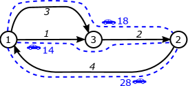
(a)

$\underline{\underline{{I}}}=\left[\begin{tabular}[]{c c c c}0&0&0&1\\ 0&1&0&0\\ 1&0&1&0\end{tabular}\right]$ $\underline{\underline{{E}}}=\left[\begin{tabular}[]{c c c c}1&0&1&0\\ 0&0&0&1\\ 0&1&0&0\end{tabular}\right]$ $\underline{{q}}=\left[\begin{tabular}[]{c}14\\ 32\\ 18\\ 28\end{tabular}\right]$ $\underline{\underline{{T}}}=\left[\begin{tabular}[]{c c c}0&32&0\\ 28&0&0\\ 0&0&0\end{tabular}\right]$ $\underline{\underline{\underline{{Q}}}}=\ \$

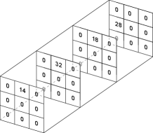
(b)

Figure 1: Example of a simple network (a) with the associated tools describing the topology and the traffic (b).

2.2 Structure of the graph and of the traffic

The structure of the graph is given by the incidence and excidence matrices denoted respectively $\underline{\underline{{I}}}$ and $\underline{\underline{{E}}}$ of size $|V|\times|L|$. These matrices describe the relations between the nodes and the edges, such that, for every $(k,l)\in V\times L$,

$$\begin{array}[]{ll}I^{l}_{k}&=\left\{\begin{array}[]{ll}1&\mbox{if the link $l$ is arriving to the node $k$},\\ 0&\mbox{otherwise},\\ \end{array}\right.\\ \\ E^{l}_{k}&=\left\{\begin{array}[]{ll}1&\mbox{if the link $l$ is starting from the node $k$},\\ 0&\mbox{otherwise}.\\ \end{array}\right.\\ \end{array}$$ (2)

Note that in graph theory, it is customary to name the difference $(\underline{\underline{{I}}}-\underline{\underline{{E}}})$ as Incidence Matrix; however we need both matrices separately in this work.

Let us also define the tensors $\underline{\underline{\underline{{I_{1}}}}}$ and $\underline{\underline{\underline{{I_{2}}}}}$ (resp. $\underline{\underline{\underline{{E_{1}}}}}$ and $\underline{\underline{\underline{{E_{2}}}}}$) corresponding to the replication of $\underline{\underline{{I}}}$ (resp. $\underline{\underline{{E}}}$) such that,

$$\begin{array}[]{rl}(\forall m\in V)&(I_{1})^{l}_{km}=\left\{\begin{array}[]{l l}1&\mbox{if link $l$ is arriving to node $k$,}\\ 0&\mbox{otherwise,}\\ \end{array}\right.\\ (\forall k\in V)&(I_{2})^{l}_{km}=\left\{\begin{array}[]{l l}1&\mbox{if link $l$ is arriving to node $m$,}\\ 0&\mbox{otherwise.}\\ \end{array}\right.\\ \end{array}$$ (3)

Using these notations, we relate the LODM $\underline{\underline{\underline{{Q}}}}$ to the classical OD matrix $\underline{\underline{{T}}}$ of size $|V|\times|V|$ where each element $T_{ij}$ contains the traffic flow originating from the node $i$ and having $j$ for destination as follows:

$$\underline{\underline{{T}}}=\sum_{\bullet\bullet l}\underline{\underline{\underline{{E_{1}}}}}\circ\underline{\underline{\underline{{Q}}}}=\sum_{\bullet\bullet l}\underline{\underline{\underline{{I_{2}}}}}\circ\underline{\underline{\underline{{Q}}}}.$$ (4)

We denote by $\underline{{O}}$ (resp. $\underline{{D}}$) the origin (resp. destination) vector, of size $|V|$ as the sum of $\underline{\underline{{T}}}$ over the second (resp. first) dimension. It represents the flows originating (or having for destination) each node of the graph. Formally,

$$\left\{\begin{array}[]{l}\underline{{D}}=(\sum_{i\bullet}\underline{\underline{{T}}})^{\top},\\ \underline{{O}}=\sum_{\bullet j}\underline{\underline{{T}}}.\end{array}\right.$$ (5)

2.3 Model, Measures and Estimates

For this problem, we consider an urban road network composed of major roads, ignoring residential and service streets, seldom equipped with traffic sensors.

The set of users with their trajectories on those major roads, are represented through the tensor $\underline{\underline{\underline{{Q}}}}$, as described above and that we wish to estimate.

For this estimation, we first assume that every road is equipped with a magnetic loop, counting the number of cars using it. It implies therefore that every element in $\underline{{{q}}}$ is known. This assumption is realistic in our case considering major roads only. The magnetic loops are usually subject to counting errors and it is modelled here by a noise $\underline{{\varepsilon}}$. Hence the measured quantity $\underline{{q}}$ reads:

$$\underline{{{q}}}=\underline{{q}}^{\star}+\underline{{\varepsilon}}$$ (6)

where $\underline{{q}}^{\star}$ is the true traffic volumes.

Second, we also assume that the proportion of Bluetooth equipped vehicle can vary with each possible pair of OD but that it doesn’t change along a trajectory (the tracking devices are not turned off and on while the car is running). This assumption allows us to define an OD-dependant penetration rate $\underline{\underline{{\eta_{o}}}}$ of size $|V|\times|V|$. Experiments in Brisbane have shown that the average Bluetooth penetration rate is around 25% [laharotte_spatiotemporal_2015]. Moreover, $\underline{\underline{\underline{{B}}}}$ appears as a noisy version of $\underline{\underline{\underline{{Q}}}}^{\star}$ for which the noise level depends on the penetration rate. The relation between the tensors $\underline{\underline{\underline{{B}}}}$ to $\underline{\underline{\underline{{Q}}}}^{\star}$ can thus be modelled by a Poisson law, typically involved in counting processes. This leads to a model

$$(\forall i,j,l\in V\times V\times L)\quad B_{ij}^{l}=\mathcal{P}((\eta_{o})_{ij}Q_{ij}^{\star l}).$$ (7)

3 Variational Approach

Instead of using the traditional four-steps model resolution, iterating over a process involving a priori information, modelling of the traffic, estimating the variables of interest, comparing to the observed measures and tuning the models, we propose here the use of a variational approach. Both our knowledge of the network and of the traffic states are included within an objective function that combines together five terms to be jointly minimised.

3.1 Objective Function

The terms of the objective functions can be classified in three types: The first type, composed of functions 3.1.1, 3.1.2 and 3.1.3, is aiming for consistency between the measures and the estimate. The second type, with function 3.1.4, stems from the topology of the network. The third and last type, with function 3.1.5, comes from an additional assumption based on our knowledge of transport networks.

3.1.1 Traffic Count Data Fidelity $f_{TC}$

Ensuring the consistency with traffic counts would require that Eq. (6) is satisfied. Noting that:

$${\underline{{q}}^{\star}}=\sum_{ij\bullet}\underline{\underline{\underline{{Q}}}}^{\star}$$ (8)

and assuming a random unbiased Gaussian noise $\underline{{\varepsilon}}$ for the magnetic loops, as in Eq. (6), the constraint of Eq (8) can be released and leads to the following function:

$$f_{TC}(\underline{\underline{\underline{{Q}}}})=\|\underline{{{q}}}-\sum_{ij\bullet}\underline{\underline{\underline{{Q}}}}\|^{2}.$$ (9)

3.1.2 Poisson Bluetooth Sampling Data Fidelity $f_{P}$

Second, the consistency with Bluetooth measures, as modelled in Equation (7) requires the knowledge of the OD-dependent penetration rate $\underline{\underline{{\eta_{o}}}}$. This information, of size $|V|\times|V|$, is not directly available from $\underline{{q}}$ and $\underline{\underline{\underline{{B}}}}$, therefore we introduce an approximation of this penetration rate of size $|L|$, noted $\underline{{\eta}}$ and calculated as:

$$\underline{{\eta}}=\frac{\underline{{{q}}}}{\sum_{i,j,\bullet}\underline{\underline{\underline{{B}}}}}.$$ (10)

The resulting data fidelity term, denoted $f_{P}$, models the minus log-likelihood associated with the Poisson model [combettes_douglas-rachford_2007]:

$$f_{P}(\underline{\underline{\underline{{Q}}}})=\sum_{ijl}\psi\left(B_{ij}^{l},\eta^{l}Q_{ij}^{l}\right)$$ (11)

where, for every $(u,v)\in\mathbb{R}^{2}$,

$$\psi(u,v)=\begin{cases}-u\log v+v&\mbox{if}\;\;v>0\;\;\mbox{and}\;\;u>0,\\ v&\mbox{if}\;\;v\geq 0\;\;\mbox{and}\;\;u=0,\\ +\infty&\mbox{otherwise}.\\ \end{cases}$$ (12)

3.1.3 Definition Domain Constraint $f_{C}$

Third, another term ensuring data consistency models that the total flow should be greater than the flow of Bluetooth enabled vehicles. It consists thus in imposing that $\underline{\underline{\underline{{Q}}}}$ belongs to the following convex set $C$:

$$C=\big{\{}\underline{\underline{\underline{{Q}}}}=\big{(}{Q}_{ij}^{l}\big{)}_{(ijl)\in V\times V\times L}\in\mathbb{R}^{|V|\times|V|\times|L|}\;|\;{Q}_{ij}^{l}\geq{B}_{ij}^{l}\big{\}}.$$ (13)

The corresponding convex function is the indicator function $\iota_{C}$:

$$f_{C}(\underline{\underline{\underline{{Q}}}})=\iota_{C}(\underline{\underline{\underline{{Q}}}})=\begin{cases}0&\mbox{\ if\ }\;\;\underline{\underline{\underline{{Q}}}}\in C,\\ +\infty&\mbox{\ otherwise.}\end{cases}$$ (14)

3.1.4 Kirchhoff’s Law $f_{K}$

This property is the classical law for flows on network, the Kirchhoff’s law, describing the conservation of cars at intersections. It takes into account the network topology. It requires that, for each OD pairs and at every node, the number of cars is conserved when properly accounting for origins and destinations. For every origin $i\in V$, destination $j\in V$ and node $k\in V$ of the network, this yields to,

$$\sum_{l}E^{l}_{k}Q^{l}_{ij}-\underbrace{\delta_{ik}T_{ij}}_{\begin{subarray}{c}\textrm{origin}\\ \textrm{(source)}\end{subarray}}=\sum_{l}I^{l}_{k}Q_{ij}^{l}-\underbrace{\delta_{jk}T_{ij}}_{\begin{subarray}{c}\textrm{destination}\\ \textrm{(sink)}\end{subarray}}.$$ (15)

This constraint can then be summarized as

$$\big{(}\forall(i,j,k)\in V^{3}\big{)}\quad\sum_{l}A^{l}_{ijk}Q^{l}_{ij}=0$$ (16)

where the $|V|\times|V|\times|V|\times|L|$ tensor $\underline{\underline{\underline{\underline{A}}}}$ is defined as

$$\big{(}\forall(i,j,k,l)\in V^{3}\times L\big{)}\quad A^{l}_{kij}=\left(E^{l}_{k}-I^{l}_{k}\right)-\left(\delta_{ik}-\delta_{jk}\right)E^{l}_{i}.$$ (17)

It results in a convex function to be minimised:

$$f_{K}(\underline{\underline{\underline{{Q}}}})=\sum_{ijk}\Big{(}\sum_{l}A^{l}_{ijk}Q^{l}_{ij}\Big{)}^{2}.$$ (18)

Compared to our previous works [michau_estimating_2015-1, michau_estimating_2015], here the Kirchhoff’s law is applied per OD pairs and not simply at a global scale. Indeed, the Kirchhoff’s law needs also to be satisfied at each node, independently of the origin and destination of the cars. Satisfying this global Kirchhoff’s law of [michau_estimating_2015-1, michau_estimating_2015] is a consequence of the one used here.

3.1.5 Total Variation $f_{TV}$

Finally, from a transport perspective it seems realistic to assume that for two paths having close origins (resp. destinations) and same destination (origin), the trajectories in the network should be correlated (e.g., use of similar roads). Such property can be written as

$$(\forall i\sim i^{\prime})(\forall j\in V)(\forall l\in L)\qquad Q_{ij}^{l}\sim Q_{i^{\prime}j}^{l}$$ (19)

$$(\forall j\sim j^{\prime})(\forall i\in V)(\forall l\in L)\qquad Q_{ij}^{l}\sim Q_{ij^{\prime}}^{l}$$ (20)

In order to be used in a variational approach these relationships can be gathered within the convex function $f_{TV}$ defined as the total variation:

$$f_{TV}(\underline{\underline{\underline{{Q}}}})=\sum_{i\sim\mathcal{N}_{i^{\prime}}}\sum_{j,l}\omega_{ii^{\prime}}|Q_{ij}^{l}-Q_{i^{\prime}j}^{l}|+\sum_{j\sim\mathcal{N}_{j^{\prime}}}\sum_{i,l}\omega_{jj^{\prime}}|Q_{ij}^{l}-Q_{ij^{\prime}}^{l}|$$ (21)

where $\mathcal{N}_{i^{\prime}}$ models the neighbourhood of $i^{\prime}$ and where $\omega_{ii^{\prime}}$ are positive weights on edges detailed later. The use of the $\ell_{1}$-norm is justified for its edge preservation properties. Indeed, it has been shown in [chambolle_introduction_2010, couprie_dual_2013] that the $\ell_{1}$-norm is adapted for cases where one seeks for spatial correlations while allowing some irregularities, e.g., edges, in image analysis. From a traffic perspective, we want to encourage users from similar origin (resp. destination) and with same destination (resp. origin) to use similar routes, but also want to allow some irregularities, e.g., for nodes in between two major roads where both could be a possible choice. Those nodes can be interpreted as edges in image analysis.

Equation (21) can further be simplified using a weighted effective incidence matrix, denoted $\underline{\underline{{J}}}$, defined as

$$\big{(}\forall(k,l)\in V\times L\big{)}\qquad J_{k}^{l}=W^{l}(I_{k}^{l}-E_{k}^{l})$$ (22)

and thus having a size $|V|\times|L|$, where each element $W^{l}$ denotes the weight for the link $l$. For this work we choose the following vector $\underline{{W}}$ of size $|L|$:

$$\big{(}\forall l\in L\big{)}\qquad W^{l}=e^{-\frac{d_{l}}{d_{0}}}$$ (23)

where $d_{l}$ models the length of the link $l$ and $d_{0}$ is the average distance of the nodes. For the simulated network:

$$d_{0}=\sqrt{\frac{\mbox{GridWidth}\cdot\mbox{GridHeight}}{|V|}}.$$ (24)

Note that $W^{l}=\omega_{km}$ if $l$ is a link between $k$ and $m$.

Eq. (21) can then be rewritten as

$$f_{TV}(\underline{\underline{\underline{{Q}}}})=\sum_{l}\|\underline{\underline{{J}}}^{\top}\underline{\underline{{Q}}}^{l}\|_{1}+\sum_{l}\|\underline{\underline{{J}}}^{\top}(\underline{\underline{{Q}}}^{l})^{\top}\|_{1}.$$ (25)

where $\underline{\underline{{Q}}}^{l}$ models the $l$-th extracted matrix from $\underline{\underline{\underline{{Q}}}}$. Its dimension is thus $|V|\times|V|$.

3.2 Algorithm

To sum up, the objective is to find an estimate of $\underline{\underline{\underline{{Q}}}}^{\star}$ satisfying

$${\underline{\underline{\underline{{\widehat{Q}}}}}}\in\underset{\underline{\underline{\underline{{Q}}}}}{\mathrm{Argmin}\,}\big{\{}\gamma_{TC}f_{TC}+\gamma_{P}f_{P}+\gamma_{C}f_{C}\\ +\gamma_{K}f_{K}+\gamma_{TV}f_{TV}\big{\}}$$ (26)

where $\gamma_{\cdot}$ are positive weights applied to the objectives and model their relative importance within the global objective.

All the five functions involved in Eq. (26) follow the usual assumptions required when dealing with convex optimisation tools: they are convex, lower-semicontinuous (l.s.c.) and proper. Moreover, both the functions $f_{TC}$ and $f_{K}$ are differentiable and their gradients are given below:

$$\nabla f_{TC}(\underline{\underline{\underline{{Q}}}})=\left(\left(-2\left(q^{l}-\sum_{k,m}Q_{km}^{l}\right)\right)_{ij}^{l}\right)_{(ijl)\in V\times V\times L}$$ (27)

and

$$\nabla f_{K}(\underline{\underline{\underline{{Q}}}})=\left(\left(2\sum_{k}A^{l}_{jik}\ \sum_{e}A^{e}_{ijk}\ Q^{e}_{ij})\right)^{l}_{ij}\right)_{(ijl)\in V\times V\times L}.$$ (28)

Their Lipschitz constants are denoted $\beta_{TC}$ and $\beta_{K}$ respectively [pustelnik_wavelet-based_2016]. The other three functions however are not differentiable and $f_{TV}$ involves a linear transformation $H$ such as:

$$f_{TV}(\underline{\underline{\underline{{Q}}}})=\|H(\underline{\underline{\underline{{Q}}}})\|_{1}$$ (29)

where $H$ satisfies:

$$H\colon \mathbb{R}^{|V|\times|V|\times|L|} \to \ \mathbb{R}^{|L|\times|V|\times|L|}\times\mathbb{R}^{|L|\times|V|\times|L|}$$ (30)

$$\underline{\underline{\underline{{Q}}}} \mapsto \ \Big{(}\big{(}\underline{\underline{{J}}}^{\top}\underline{\underline{{Q}}}^{l}\big{)}_{l\in L},\big{(}\underline{\underline{{J}}}^{\top}(\underline{\underline{{Q}}}^{l})^{\top}\big{)}_{l\in L}\Big{)}$$

and whose adjoint is

$$H^{*}\colon (\underline{\underline{\underline{{R}}}},\underline{\underline{\underline{{S}}}}) \mapsto \ \Big{(}\underline{\underline{{J}}}\;\underline{\underline{{R}}}^{l}\Big{)}_{l\in L}+\Big{(}(\underline{\underline{{J}}}\;\underline{\underline{{S}}}^{l})^{\top}\Big{)}_{l\in L}.$$ (31)

In the following, we denote $\chi_{H}$ the norm of this operator. For further details about the way to compute this norm, the reader can refer to [pustelnik_wavelet-based_2016].

Choose: $\gamma_{TC}\geq 0,\quad\gamma_{K}\geq 0,\quad\gamma_{TV}\geq 0,\quad\gamma_{P}\in[0,1],\quad\gamma_{D}\in[0,1]$
Compute: $\chi_{H},\quad\beta=\gamma_{TC}\beta_{TC}+\gamma_{K}\beta_{K}$,  if $\gamma_{TV}=0$, $\quad\tau=\frac{1.99}{\beta}$, else choose $(\tau,\sigma)$ such as $\tau=\frac{0.9}{\frac{\beta}{2}+\sigma\chi_{H}}\in[\frac{2}{3}\sigma,\frac{3}{2}\sigma]$
Set : $\underline{\underline{\underline{{Q}}}}^{0}=\underline{\underline{\underline{{0}}}}$, $\quad(\underline{\underline{\underline{{R}}}}^{0},\underline{\underline{\underline{{S}}}}^{0})=(\underline{\underline{\underline{{0}}}},\underline{\underline{\underline{{0}}}})$

For $k=0$,… :
     1. $\widetilde{\underline{\underline{\underline{{Q}}}}}^{k+1}=\underline{\underline{\underline{{Q}}}}^{k}-\tau\big{(}\gamma_{TC}\nabla f_{TC}(\underline{\underline{\underline{{Q}}}}^{k})+\gamma_{K}\nabla f_{K}(\underline{\underline{\underline{{Q}}}}^{k})\big{)}-\tau H^{*}(\underline{\underline{\underline{{R}}}}^{k},\underline{\underline{\underline{{S}}}}^{k})$
     2. $\underline{\underline{\underline{{Q}}}}^{k+1}=\mathrm{prox}_{\gamma_{C}f_{C}}\Bigg{(}\mathrm{prox}_{\tau\gamma_{P}f_{P}}\Big{(}\widetilde{\underline{\underline{\underline{{Q}}}}}^{k+1}\Big{)}\Bigg{)}$
     3. $\big{(}\widetilde{\underline{\underline{\underline{{R}}}}}^{k+1},\widetilde{\underline{\underline{\underline{{S}}}}}^{k+1}\big{)}=\sigma H(2\widetilde{\underline{\underline{\underline{{Q}}}}}^{k+1}-\underline{\underline{\underline{{Q}}}}^{k})+\big{(}\underline{\underline{\underline{{R}}}}^{k},\underline{\underline{\underline{{S}}}}^{k}\big{)}$
     4. $\Big{(}\underline{\underline{\underline{{R}}}}^{k+1},\underline{\underline{\underline{{S}}}}^{k+1}\Big{)}=\Big{(}\widetilde{\underline{\underline{\underline{{R}}}}}^{k+1},\widetilde{\underline{\underline{\underline{{S}}}}}^{k+1}\Big{)}-\sigma\cdot\mathrm{prox}_{\gamma_{TV}/\sigma,\ell_{1}}\left(\frac{1}{\sigma}\widetilde{\underline{\underline{\underline{{R}}}}}^{k+1},\frac{1}{\sigma}\widetilde{\underline{\underline{\underline{{S}}}}}^{k+1}\right)$
Stop if:
     $\frac{\|\underline{\underline{\underline{{Q}}}}^{k+1}-\underline{\underline{\underline{{Q}}}}^{k}\|_{2}}{\|\underline{\underline{\underline{{Q}}}}^{k+1}\|_{2}}<10^{-6}$ OR $k>10^{5}$

Algorithm 1 Primal Dual algorithm

This optimisation problem is solved by means of a primal-dual proximal algorithm, as in [vu_splitting_2011, combettes_primal-dual_2011, condat_primal-dual_2013, komodakis_playing_2015], which is particularly suited when the objective combines differentiable and non-differentiable functions along with linear operators. In such an iterative scheme, the non-differentiable functions are involved through their proximity operator [moreau_proximite_1965] defined as:

$$(\forall u\in\mathcal{H})\qquad\mathrm{prox}_{f}(u)=\operatorname{arg}\min_{x\in\mathcal{H}}f(x)+\frac{1}{2}\|u-x\|_{2}^{2}$$ (32)

where $\mathcal{H}$ denotes a real Hilbert space and $f$ a convex, l.s.c., proper function from $\mathcal{H}$ to $]-\infty,+\infty]$. For further details on proximal algorithms, the reader could refer to [combettes_proximal_2010, bauschke_convex_2011, parikh_proximal_2013].

The proximity operator of the indicator of the convex set $C$ has a closed form expression as a projection [theodoridis_adaptive_2011]:

$$\mathrm{prox}_{\gamma_{C}f_{C}}(\underline{\underline{\underline{{Q}}}})=\left\{\begin{array}[]{ll}P_{C}(\underline{\underline{\underline{{Q}}}})=\max(\underline{\underline{\underline{{Q}}}},\underline{\underline{\underline{{B}}}})&\mbox{if }\gamma_{C}>0\\ \underline{\underline{\underline{{Q}}}}&\mbox{if }\gamma_{C}=0.\\ \end{array}\right.$$ (33)

The proximity operator of the function, $f_{P}$, also have a closed form expression [combettes_douglas-rachford_2007]:

$$\mathrm{prox}_{\gamma_{P}f_{P}}(\underline{\underline{\underline{{Q}}}})$$ (34)

$$=\Big{(}\mathrm{prox}_{\gamma_{P}\psi}(B_{ij}^{l},\eta^{l}Q_{ij}^{l})\Big{)}_{(ijl)\in V\times V\times L}$$

$$=\Bigg{(}\frac{Q_{ij}^{l}-\gamma_{P}\eta^{l}+\sqrt{|Q_{ij}^{l}-\gamma_{P}\eta^{l}|^{2}+4\gamma_{P}B_{ij}^{l}}}{2}\Bigg{)}_{(ijl)\in V\times V\times L}.$$

The proximal operator of the sum of these two functions satisfies the following property [chaux_nested_2009]:

$$\mathrm{prox}_{\gamma_{C}f_{C}+\gamma_{P}f_{P}}(\underline{\underline{\underline{{Q}}}})=P_{C}(\mathrm{prox}_{\gamma_{P}f_{P}}(\underline{\underline{\underline{{Q}}}})).$$ (35)

Last, the $\ell_{1}$-norm, applied to $H$, as in Eq. (29), also has a closed form expression for its proximity operator [chaux_variational_2007, pustelnik_parallel_2009, donoho_-noising_1995, combettes_signal_2005]:

$$\mathrm{prox}_{\gamma_{TV}\|\cdot\|_{1}}(\underline{\underline{\underline{{R}}}},\underline{\underline{\underline{{S}}}})=\Bigg{(} \mathrm{sign}(\underline{\underline{\underline{{R}}}})\ \max\{|\underline{\underline{\underline{{R}}}}|-\gamma_{TV},0\},$$ (36)

$$\mathrm{sign}(\underline{\underline{\underline{{S}}}})\ \max\{|\underline{\underline{\underline{{S}}}}|-\gamma_{TV},0\}\Bigg{)}.$$

The primal-dual proximal iterations designed for minimizing Eq. (26) are described in Algorithm 1. Under some technical assumptions regarding the domain of definition and the following condition [condat_primal-dual_2013, theorem (3.1)]:

$$\frac{1}{\tau}-\sigma\chi_{H}\geq\frac{\beta}{2},$$ (37)

where the $\beta=\gamma_{TC}\beta_{TC}+\gamma_{K}\beta_{K}$ denotes the Lipschitz constant of $\gamma_{TC}f_{TC}+\gamma_{K}f_{K}$ and $\sigma>0$, the sequence $\big{(}\underline{\underline{\underline{{Q}}}}^{k+1}\big{)}_{k\in\mathbb{N}}$ converges to a minimizer of Eq. (26).

4 Simulated Case Study

4.1 Experimental setup

4.1.1 Simulation context

To test and validate the proposed method, a simplified road network model has been created. This has been preferred to a real case study for three reasons: tractability, the possibility to access the ground truth and the opportunity to explore the behaviour of the method for varied conditions. However, the number of nodes, the connectivity, the number of users and their OD patterns have been chosen to be consistent with those of a real networks.

The number of nodes of the simulated network is $|V|=50$ nodes. This number is kept relatively low to allow for a thorough exploration of the possible weights $\gamma_{\cdot}$ of problem (26). For comparison, the Brisbane Bluetooth scanner network has around $900$ intersections equipped with vehicle identification devices. Other works on ODM estimation consider often few tens of nodes ($\propto 100$ OD flows) [djukic_advanced_2015] while very recent works considered up to $300$ nodes [perrakis_bayesian_2015].

For the simulation, nodes are first located randomly on a grid and then links are created while aiming for an average connectivity of 6, a value consistent with that of real road networks [porta_network_2006]. This is done first, by means of a minimum spanning tree (computed by the Kruskal’s algorithm [cormen_algorithms_2009]), then, by adding links randomly to the nodes with lower degree (sum of in and out edges) provided that the added links do not cross or repeat an existing one.

The number of users is fixed to $N=10^{5}$. This leads to an mean flow per link of 3000 users. In big cities, it would correspond to around one hour of traffic during peak hours. Each node $i$ has a probability $p_{O}(i)$ of being an origin and similarly we define $p_{D}(j)$ the probability of node $j$ to be a destination. Thus $\underline{{p_{O}}}$ and $\underline{{p_{D}}}$ satisfy:

$$\left\{\begin{array}[]{l}\underline{{D}}=\mathbb{E}(N\times\underline{{p_{D}}}),\\ \underline{{O}}=\mathbb{E}(N\times\underline{{p_{O}}}).\\ \end{array}\right.$$ (38)

An origin and a destination are randomly associated to each user, according to the probabilities $p_{O}$ and $p_{D}$. We simulate a preferred direction of travel, consistent with the trends observed in urban context (mostly due to commuters). To this end, $p_{O}$ is decreasing linearly with the X-axis of the grid while $p_{D}$ is increasing linearly. The shortest path from origin to destination is then attributed to each user.

For each OD pair, a Bluetooth penetration rate is drawn from a Gaussian distribution of mean 30% and standard deviation of 10% (and truncated to be between 0 and 1). This choice accounts for the variability of the ownership distribution of Bluetooth devices (which is not known) from one node to another, depending, as an example, on the wealth of the neighbourhoods of the node. Each user has a probability equal to the Bluetooth penetration rate drawn for its OD of being equipped with a Bluetooth device. This gives us $\underline{\underline{\underline{{B}}}}$ while the full set of trajectories gives $\underline{\underline{\underline{{Q}}}}^{\star}$ for ground truth. The measured traffic flow per link $\underline{{q}}$ is obtained from $\underline{\underline{\underline{{Q}}}}^{\star}$, assuming the addition a noise $\underline{{\varepsilon}}$, for which each independent component is drawn from a Gaussian distribution ${\cal N}(0,r\cdot\underline{{q}}^{\star})$. For consistency with the noise usually measured on magnetic loops [coifman_using_1999], we take $r=5\%$. Figure 2 illustrates the simulated case study with total volumes on the links ($\underline{{q}}$) and the realisation of $p_{O}$ and $p_{D}$ for the $10^{5}$ users on the nodes.

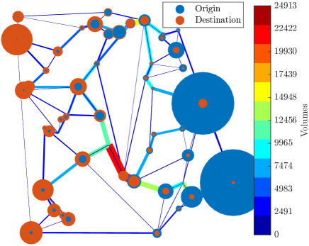
Figure 2: Simulated road networks with the projection of $\underline{{q}}$ on the links: the width is proportional to the flows, also correlated with the color. For nodes, the color distinguishes between origin (blue) and destination flows (red) and the diameter of the nodes is proportional to their value in $\underline{{p_{O}}}$ and $\underline{{p_{D}}}$.

4.1.2 Algorithmic parameters setup

As discussed in section 3.2, the objective function (26) depends on five parameters $\gamma_{\cdot}\geq 0$. It appears however that, as $f_{C}$ can only be $0$ or $\infty$, exploring $\gamma_{C}\in\{0;1\}$ is enough. Moreover, the minimum in Equation (26) is preserved by a linear operation over the four remaining parameters $\gamma_{\cdot}$, and thus we choose $\gamma_{P}\in\{0;1\}$. This would then correspond to two situations: with or without considering the data stemming from sampled trajectories in the estimation process. We then explore the space of positive real numbers for the three remaining parameters $\gamma_{\cdot}$.

For those parameters, it has been observed that, for comparison purposes, it is justified to compare scenarii for rescaled values $\gamma_{\cdot}\beta_{\cdot}$. Indeed, $\beta_{\cdot}$ depends on the setup, in particular on $\underline{{q}}$ and $\underline{\underline{\underline{{B}}}}$.

The algorithm stops if the convergence criteria is satisfied (cf. Alg. 1) or after $10^{5}$ iterations.

4.1.3 Performance evaluation

The efficiency of the estimation algorithm is assessed by comparing its results to the ground truth $\underline{\underline{\underline{{Q}}}}^{\star}$ with two indicators. First, we denote RMSE the $\ell_{2}$ norm of the error divided by the norm of the ground truth (RMSE standing for Root Mean Square Error):

$$RMSE(\widehat{\underline{\underline{\underline{{Q}}}}})=\frac{\|\widehat{\underline{\underline{\underline{{Q}}}}}-\underline{\underline{\underline{{Q}}}}^{\star}\|}{\|\underline{\underline{\underline{{Q}}}}^{\star}\|}.$$ (39)

Second, EMD refers to the Earth Movers’ Distance [rubner_earth_2000], a metric often used for image or distribution comparisons. It corresponds to the minimal cost that must be paid to transform the histogram of one image or distribution into the other.

We also provide a comparison of the estimates with two naive solutions denoted $\widehat{\underline{\underline{\underline{{Q}}}}}^{0}$ and $\widehat{\underline{\underline{\underline{{Q}}}}}^{1}$, computed as the Bluetooth LODM multiplied by the mean Bluetooth penetration rate over the whole network ($\widehat{\eta}$), or over each link ($\underline{{\eta}}$) respectively, for every $(i,j,l)\in V\times V\times L$,

$$(\widehat{{Q}}^{0})^{l}_{ij}=\widehat{\eta}\ B^{l}_{ij} \widehat{\eta}=\sum_{l}{\underline{{q}}}/\sum_{i,j,l}\underline{\underline{\underline{{B}}}},$$ where (40)

$$(\widehat{{Q}}^{1})^{l}_{ij}=\eta^{l}\ B^{l}_{ij} \eta^{l}=q^{l}/\sum_{i,j,\bullet}\underline{\underline{\underline{{B}}}}.$$ where

4.2 Results

4.2.1 Finding the best estimates

Solutions to problem (26) have been explored through a systematic exploration of the $\gamma_{\cdot}$ values within the positive real numbers. Figures 3 and 4 illustrate the evolution of the criteria RMSE (Fig. 3) and EMD (Fig. 4) as a function of one $\gamma_{\cdot}$, the others being fixed. It highlights the existence of sets of parameters $\gamma_{\cdot}$ for which the estimates have minimal criteria while being lower than the criteria of the naive estimates $\widehat{\underline{\underline{\underline{{Q}}}}}^{0}$ and $\widehat{\underline{\underline{\underline{{Q}}}}}^{1}$. Therefore, in the following we denote by $\widehat{\underline{\underline{\underline{{Q}}}}}_{RMSE}$ the estimate $\widehat{\underline{\underline{\underline{{Q}}}}}$ minimizing the RMSE and by $\widehat{\underline{\underline{\underline{{Q}}}}}_{EMD}$ the one minimising the EMD. That is:

$$\widehat{\underline{\underline{\underline{{Q}}}}}_{RMSE}\in \underset{\widehat{\underline{\underline{\underline{{Q}}}}}}{\mathrm{Argmin}\,}RMSE(\widehat{\underline{\underline{\underline{{Q}}}}}),$$ (41)

$$\widehat{\underline{\underline{\underline{{Q}}}}}_{EMD}\in \underset{\widehat{\underline{\underline{\underline{{Q}}}}}}{\mathrm{Argmin}\,}EMD(\widehat{\underline{\underline{\underline{{Q}}}}}).$$ (42)

Figure 5 represents the distribution of the elements in $\widehat{\underline{\underline{\underline{{Q}}}}}^{0}$, $\widehat{\underline{\underline{\underline{{Q}}}}}^{1}$, $\widehat{\underline{\underline{\underline{{Q}}}}}_{RMSE}$, $\widehat{\underline{\underline{\underline{{Q}}}}}_{EMD}$ as histograms, superposed to the ground truth $\underline{\underline{\underline{{Q}}}}^{\star}$ for comparison. As one could have expected from Eq (40), $\widehat{\underline{\underline{\underline{{Q}}}}}^{0}$ contains only multiples of the penetration rate value $\widehat{\eta}$. It has therefore a higher EMD value than other estimates.

For those four same estimates, Table 1 presents the values for RMSE, EMD, $f_{TC}$ (consistency with observed counts) and $f_{K}$ (conformity with Kirchhoff’s law). These two functions are chosen because they are the most important from a transport perspective point-of-view. When applicable, the corresponding values for the $\gamma_{\cdot}$ are indicated. The table illustrates that $\widehat{\underline{\underline{\underline{{Q}}}}}^{0}$ is a good solution from a transport perspective as it has low values for $f_{TC}$ and $f_{K}$ but is the worst performing when it is compared to the ground truth $\underline{\underline{\underline{{Q}}}}^{\star}$ (both for EMD and RMSE). On the opposite, $\widehat{\underline{\underline{\underline{{Q}}}}}^{1}$ has better RMSE and EMD values than $\widehat{\underline{\underline{\underline{{Q}}}}}^{0}$ but performs poorly on the relevant transport indicators. Hence it is justified to actually solve problem (26) as none of the naive solutions bring satisfying results. While doing so, both $\widehat{\underline{\underline{\underline{{Q}}}}}_{RMSE}$ and $\widehat{\underline{\underline{\underline{{Q}}}}}_{EMD}$ give similar results in term of comparison to ground truth. As one might expect, their performances with respect to the transport indicators are consistent with the weights applied to the corresponding functions: The solution $\widehat{\underline{\underline{\underline{{Q}}}}}_{RMSE}$ is reached for higher $\gamma_{TC}$ and, therefore, performs much better on the $f_{TC}$ criterion while $\widehat{\underline{\underline{\underline{{Q}}}}}_{EMD}$ has a relatively higher $\gamma_{K}$ and hence satisfies the Kirchhoff’s law better. The question of which solution is the best partly depends on the reliability of the link counts (if the noise is high, satisfying perfectly $f_{TC}$ might not be relevant). Anyway, choosing between the two amounts to choosing the best $\gamma_{\cdot}$, a question left for future work.

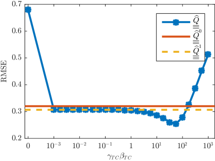
Figure 3: RMSE as a function of $\gamma_{TC}\ \beta_{TC}$ for $\gamma_{K}=\gamma_{TV}=0$ and $\gamma_{C}=\gamma_{P}=1$. Note that the first point on the left is for $\gamma_{TC}\ \beta_{TC}=0$, to be distinguished from the logarithmic scale from the second point and after.

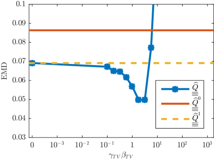
Figure 4: EMD as a function of $\gamma_{TV}\ \beta_{TV}$ for $\gamma_{K}=0$ and $\gamma_{TC}=\gamma_{C}=\gamma_{P}=1$. Again, note that the first point on the left is for $\gamma_{TV}\ \beta_{TV}=0$ whereas the rest is drawn on a logarithmic scale.

Table 1: Results for LODM estimates: the two naive solution and the ones minimizing RMSE and the EMD

	$\gamma_{TC}$	$\gamma_{K}$	$\gamma_{TV}$	RMSE	EMD	$f_{K}$	$f_{TC}$
$\widehat{\underline{\underline{\underline{{Q}}}}}^{0}$				0.320	0.086	0	55
$\widehat{\underline{\underline{\underline{{Q}}}}}^{1}$				0.307	0.069	1142	84
$\widehat{\underline{\underline{\underline{{Q}}}}}_{RMSE}$	31.6	0.008	0.015	0.239	0.047	289	1
$\widehat{\underline{\underline{\underline{{Q}}}}}_{EMD}$	1	0.025	0.027	0.244	0.045	133	28

4.2.2 Impact of each objective

If it appears from these results that it is justified to solve problem (26), the question of the importance of each function can be raised. To answer such a question, Tables 2(a) (resp. (b)) summarises the best RMSE values (resp. EMD) when only the objectives indexed by the rows and column are not set to zeros. Thus diagonal elements correspond to a single term in the objective function while the four others are set to zero and non diagonal elements involve at most the two terms indexed by the row and column. For example, element (1,2) of Table 2(a) corresponds to the best value of RMSE achieved for $\gamma_{TV}=\gamma_{P}=\gamma_{C}=0$ and values of $\gamma_{K}$ and $\gamma_{TC}$ evaluated on a grid. For those tables, light-grey cells correspond to estimates that could not outperform the naive estimates, and darker grey elements, cases for which Algorithm 1 reached the $100000$ steps limit without convergence.

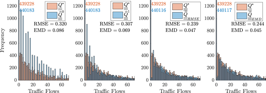
Figure 5: Distribution as histograms of the elements in $\widehat{\underline{\underline{\underline{{Q}}}}}^{0}$, $\widehat{\underline{\underline{\underline{{Q}}}}}^{1}$, $\widehat{\underline{\underline{\underline{{Q}}}}}_{RMSE}$, $\widehat{\underline{\underline{\underline{{Q}}}}}_{EMD}$ (in blue) superposed to the ground truth $\underline{\underline{\underline{{Q}}}}^{\star}$ (in red).

The observation of both tables (for RMSE and EMD) leads to the conclusion that neither term gives satisfactory results by itself. None of the diagonal elements outperform the naive estimates. To improve on those values, one must involve the Poisson assumption and either the traffic counts function or the Kirchhoff’s law. This means that one cannot obtain a good estimate of the traffic flows while there are not at least one term ensuring data fidelity along with a regularization term. The fact that the Poisson function seems to be the most important can be expected as $\underline{\underline{\underline{{B}}}}$ brings the most information and confirms the importance of probe trajectories to solve such traffic problem.

Thus in a second step, the Poisson function has been imposed ($\gamma_{P}=1$) with either one or two extra functions and similar results are gathered in Tables 3(a) and (b). In those tables, the indicator function corresponding to the projection on the convex set $f_{C}$ has also been imposed ($\gamma_{C}=1$) for three reasons: First its additional computational cost is negligible compared to the other functions, second, it accelerates the convergence speed of the algorithm by reducing the number of steps required while having little impact on the values of the criteria at convergence. Last, it corresponds to the weakest assumption of our model: that the total flow is greater than the measured probe trajectories.

In this second scenario (with $\gamma_{P}=\gamma_{C}=1$ and one or two additional functions), any estimate performs better than the naive one but for the case where only the total variation (TV) is added. Depending on whether a minimum is sought for RMSE or for the EMD, it is either the pair Kirchhoff’s law and TV, or the pair Traffic Counts and TV, that are the best suited to complement the Poisson assumption. In any case, best results, as summarised in Table 1, are achieved when all functions are involved. However, these results might question the role of the TV: First one can not reach better results than with naive estimates if at least the Poisson assumption and another function (K or TC) are not also involved. Second, the additional computation cost in Algorithm 1 caused by the realisation of $H$, its adjoint and the proximal of the $\ell_{1}$-norm multiplies by four the time needed for each iteration (convergence reached in $\sim$4 hours instead of $\sim$1 on a Core i7 laptop). However, the total variation bring a slight improvement to the results for both RMSE (0.262 to 0.239) and the EMD (0.067 to 0.045). This is probably caused by the difficulty of estimating flows not sampled at all by the probe trajectories, task to which, in this version of the problem, the total variation is the only answer.

Table 2: Best values of RMSE and EMD when only one or two constraints are considered

(a)	RMSE TC K TV P C TC 0.99 0.98 0.99 0.30 0.67 K 1 1 0.29 0.68 TV 1 0.39 0.68 P 1 0.68 C 0.68
(b)	EMD TC K TV P C TC 2.03 1.20 1.20 0.07 1.43 K 1.20 1.20 0.08 0.81 TV 1.20 0.19 0.78 P 1.20 0.81 C 0.81

Table 3: Best values of RMSE and EMD when $\gamma_{C}=\gamma_{P}=1$ and with one or two additional constraints

(a) (b)
RMSE TC K TV TC 0.27 0.26 0.26 K 0.27 0.25 TV 0.35 EMD TC K TV TC 0.067 0.067 0.046 K 0.069 0.069 TV 0.605

4.3 Results with fewer users on the networks

Finally, one might wonder whether this method, as presented in this article, can achieve similar results over smaller time periods, that is in our case, a lower number of users. In this section the main results are presented again for $N=10^{4}$ users. This correspond to an average flow of 300 vehicles per link. In a big city, this correspond to 5 to 10 minutes of traffic during peak hours. With such a low number of users we are reaching the limits of our model as $10^{4}$ users corresponds to $\sim$4 users (that is, in average, 1.3 probe trajectories) per OD. Therefore the impact of the Poisson assumption, inferring information from $\underline{\underline{\underline{{B}}}}$ decreases. Table 4 summarises the results in this case. Yet there is still a 14% improvement on the RMSE and a 30% improvement on the EMD. These results are very encouraging as even in the limit cases, the estimates achieved with the algorithm are still an improvement with respect to the naive estimates.

Table 4: Best Achieved Results with N=10 000

	$\gamma_{TC}$	$\gamma_{K}$	$\gamma_{TV}$	RMSE	EMD	$f_{K}$	$f_{TC}$
$\widehat{\underline{\underline{\underline{{Q}}}}}^{0}$				0.398	0.021	0	13.3
$\widehat{\underline{\underline{\underline{{Q}}}}}^{1}$				0.396	0.017	128	0.1
$\widehat{\underline{\underline{\underline{{Q}}}}}_{RMSE}$	1.78	0.25	0.027	0.341	0.013	10.7	9.8
$\widehat{\underline{\underline{\underline{{Q}}}}}_{EMD}$	1	0.45	0.026	0.342	0.012	5.8	13.7

5 Conclusion

We have shown that the Link dependent Origin-Destination matrix is an interesting tool for traffic representation. Moreover we have evidenced that its estimation can be performed with a primal dual algorithm and that the objective function to be minimized can be partially derived from natural properties of the problem (the consistency between measured and estimated traffic counts, the domain of definition and the Kirchhoff’s law). Then by adding a few sensible relationships, as for example, the Poisson sampling assumption and the similarities between nearby flows computed as the total variation, one can obtain from such method, estimates that outperform the naive solutions. However improvements can still be sought, especially by designing new functions. Future works will demonstrate that, if available, traffic turn fractions at intersections can be involved as an additional term to achieve even better results. Another trail for developing this problem is to look for an online algorithm as the one presented in [combettes_stochastic_2015, Section 5.2]. Last, one could think about implementing time dependencies. This could be done by adding new relationships that would link successive estimations of the LODM or, alternatively, by using other methods: for example, a Kalman filter similarly to what have been done on traffic counts based ODM estimation [cremer_new_1987], or also with supplementary data (e.g., Bluetooth [barcelo_robustness_2013] or other sensors [lu_kalman_2015]).