The Mittag-Leffler Fitting of the Phillips Curve

Abstract

In this paper, a mathematical model based on the one-parameter Mittag-Leffler function is proposed to be used for the first time to describe the relation between unemployment rate and inflation rate, also known as the Phillips curve. The Phillips curve is in the literature often represented by an exponential-like shape. On the other hand, Phillips in his fundamental paper used a power function in the model definition. Considering that the ordinary as well as generalised Mittag-Leffler function behaves between a purely exponential function and a power function it is natural to implement it in the definition of the model used to describe the relation between the data representing the Phillips curve. For the modelling purposes the data of two different European economies, France and Switzerland, were used and an “out-of-sample” forecast was done to compare the performance of the Mittag-Leffler model to the performance of the power-type and exponential-type model. The results demonstrate that the ability of the Mittag-Leffler function to fit data that manifest signs of stretched exponentials, oscillations or even damped oscillations can be of use when describing economic relations and phenomenons, such as the Phillips curve.

Institute of Control and Informatization of Production Processes
BERG Faculty, Technical University of Kosice
Nemcovej 3, 042 00 Kosice, Slovak Republic
phone number: +421556025143
e-mail: tomas.skovranek@tuke.sk

Keywords: Econometric modelling; Identification; Phillips curve; Mittag-Leffler function

1 Introduction

It is “because of” or “thanks to” Paul Anthony Samuelson and Robert Merton Solow (Samuelson and Solow, 1960), that the economists all around the world call the negative correlation between the rate of wage change (or the price inflation rate) and unemployment rate the Phillips curve (PC). It is lesser-known, that the idea occurred more than 30 years before publishing the famous paper of Alban William Housego Phillips (Phillips, 1958), in the work by Irving Fisher (Fisher, 1926). And Fisher was not the only one who would deserve such an important “discovery” be named after him. Arthur Joseph Brown in his book (Brown, 1955), published 3 years before Phillips paper, precisely described the inverse relation between the wage and price inflation and the rate of unemployment. Also Richard George Lipsey (Lipsey, 1960) played an important role by the birth, creation of the theoretical foundations and popularisation of the PC. Samuelson and Solow in their paper (Samuelson and Solow, 1960) for the first time mention policy implications. In the empirical studies (Brown, 1955; Phillips, 1958; Lipsey, 1960) for the United Kingdom, and (Bowen, 1960; Samuelson and Solow, 1960; Bodkin, 1966) for the United States, the inverse relationship between the rate of wage change and the unemployment rate was proven. The PC was in its beginnings widely used by the policy-makers to exploit the trade-off to reduce unemployment at a small cost of additional inflation - “sacrifice ratio”.

Since then the PC has been studied, extended and re-formulated by many authors. One of the “modern” forms of the PC is represented by models in which expectations are not anchored in backward-looking behaviour but can jump in response to current and anticipated changes in policy - the New Keynesian theory of the output-inflation tradeoff. The model called the New Keynesian Phillips Curve (NKPC) builds, among others, on the works of Taylor (Taylor, 1979, 1980) and Calvo (Calvo, 1983), where the models of staggered contracts were developed, and on the quadratic price adjustment cost model of Rotemberg and Woodford (Rotemberg, 1982; Rotemberg and Woodford, 1997), all of which have a similar formulation as the expectations-augmented PC of Friedman and Phelps (Friedman, 1968; Phelps, 1968). The work of Clarida et al. (Clarida et al., 1999) illustrates the widely usage of this model in theoretical analysis of monetary policy. With the focus shifted from the unemployment rate to the output gap, Phillips’ relationship has become an aggregate supply curve, but the idea remains the same. McCallum (McCallum, 1997) has called it “the closest thing there is to a standard specification”. The NKPC stayed popular also in the late 90’s and at the beginning of the 21^st century as a theory for understanding inflation dynamics. In the works (Galí and Gertler, 1999; Galí et al., 2001, 2005) the NKPC was transformed into a hybrid version, that relates inflation to expected future inflation, lagged inflation and real marginal costs.

When Magnus Gustaf Mittag-Leffler in his works (Mittag-Leffler, 1903a, b) proposed a new function $E_{\alpha}(x)$, he surely did not expect how important generalisation of the exponential function $e^{x}$ he developed. The ML function and its generalisations interpolate between a purely exponential law and a power-law-like behaviour, and they arise naturally in the solution of fractional-order integro-differential equations, random walks, Lévy flights, the study of complex systems, and in other fields. In numerous works the properties, generalisations and applications of the ML-type functions were studied e.g.  (Hille and Tamarkin, 1930; Dzhrbashyan, 1966; Caputo and Mainardi, 1971; Blair, 1974; Torvik and Bagley, 1984; Samko et al., 1993; Gorenflo and Vessella, 1991; Gorenflo and Mainardi, 1996, 1997; Gorenflo et al., 2002, 2014; Kilbas and Saigo, 1995, 1996; Kilbas et al., 2004; Mainardi and Gorenflo, 1996, 2000; Srivastava and Saxena, 2001; Srivastava and Tomovski, 2009; West et al., 2003; Haubold et al., 2011; Garrappa, 2015), and computation procedures for evaluating the ML function were developed e.g. in (Gorenflo et al., 2002; Chen, 2008a, b; Podlubny, 2005, 2011; Garrappa, 2015; Matychyn, 2017).

The Mittag-Leffler (ML) function become of great use and importance not only for mathematicians, but because of its special properties and huge potential by solving applied problems it found its applicability also in the fields such as psychorheology (Blair, 1974), electrotechnics (Capelas de Oliveira et al., 2011; Petras et al., 2012; Sierociuk et al., 2013), modeling of processes such as diffusion (Maindardi, 2018), combustion (Samuel et al., 2016), universe expansion (Zeng et al., 2015), etc. The idea to use the fractional-order calculus and the ML function for modelling phenomenons from the fields of economics and econophysics was elaborated by several authors (Scalas et al., 2000; Gorenflo et al., 2001; Mainardi et al., 2000, 2002; Cartea and del Castillo-Negrete, 2007; Vilela Mendes, 2008; Garibaldi and Scalas, 2010; Skovranek et al., 2012; Tejado, 2015, 2018; Tarasov, 2016; Tarasov and Tarasova, 2017; Tarasova and Tarasov, 2018; Tarasov, 2018, 2019, 2019a, 2019b, 2019c).

In this paper the one-parameter ML function is for the first time used to model the relation between the unemployment rate and the inflation rate - the Phillips curve, and its performance is compared to the power-type model and the exponential-type model. French and Swiss econometric data are taken for the period of time 1980 - 2017 from the portal EconStats^TM (Econstats.com, 2019) to identify the PC of these economies. The dataset is split into two subsets, the “modelling” subset is used to identify the model parameters, and a shorter “out-of-sample” subset serves for evaluating the forecast-performance of the models. The performance of all three models is evaluated based on the fitting-criterion, i.e. the sum of squared errors (SSE). The results are presented in the form of figures and tables, where the SSE of the fitting curve to the “modelling” subset, SSE of the fitting curve to the “out-of-sample” subset, and SSE of the fitting curve to the complete dataset, as well as some other quality criterions for the goodness-of-fit are listed.

The paper is organised as follows. Section 2 gives an overview of Mittag-Leffler function and its generalisations. The original Phillips curve as well as the and Mittag-Leffler model for fitting the Phillips curve is described in Section 3. The numerical results and the discussion on the experiments can be found in Section 4. Finally, concluding remarks are given in Section 5.

2 Preliminaries: Mittag-Leffler function and its generalisations

In 1903 M. G. Mittag-Leffler (Mittag-Leffler, 1903a, b) introduced a new function $E_{\alpha}(x)$, a generalisation of the classical exponential function $e^{x}$, which is till today known as the one-parameter ML function. Using Erdélyi’s notation (Erdélyi et al., 1955), where $z$ is used instead of $x$, the function can be written as:

$$E_{\alpha}(z)=\sum_{k=0}^{\infty}\frac{z^{k}}{\Gamma(\alpha k+1)},\quad\alpha\in\mathbb{C},\,\operatorname{Re}(\alpha)>0,\,z\in\mathbb{C},$$ (1)

where $\Gamma$ denotes the (complete) Gamma function, having the property $\Gamma(n)=(n-1)!$. The one-parameter ML function and its properties were further investigated in (Mittag-Leffler, 1904, 1905; Wiman, 1905a, b; Pollard, 1948; Agarwal, 1953; Humbert, 1953; Humbert and Agarwal, 1953) followed by the generalisation to a two-parameter function of the ML-type, by some authors called the Wiman’s function (some give the credit to Agarwal). Following the Erdélyi’s handbook the formula has the form (Erdélyi et al., 1955):

$$E_{\alpha,\beta}(z)=\sum_{k=0}^{\infty}\frac{z^{k}}{\Gamma(\alpha k+\beta)},\quad\alpha,\beta\in\mathbb{C},\,\operatorname{Re}(\alpha)>0,\,\operatorname{Re}(\beta)>0,\,z\in\mathbb{C}.$$ (2)

The main properties of the above mentioned functions, and other ML-type functions, can be found in the book by Erdélyi et al. (Erdélyi et al., 1955), and a detailed overview in the book by Dzhrbashyan (Dzhrbashyan, 1966). To demonstrate the concept of generality of the ML-type functions let us point out, that the ML function for one parameter (1), is a special case of the two-parameter ML function, i.e. if we substitute $\beta=1$ in (2). Accordingly, the classical exponential function is a special case of the one-parameter ML function, where $\alpha=1$:

$$E_{\alpha,1}(z)=\sum_{k=0}^{\infty}\frac{z^{k}}{\Gamma(\alpha k+1)}\equiv E_{\alpha}(z),$$

$$E_{1}(z) =\sum_{k=0}^{\infty}\frac{z^{k}}{\Gamma(k+1)}=\sum_{k=0}^{\infty}\frac{z^{k}}{k!}=e^{z}.$$

In 1971 the generalisation of the two-parameter function of the ML-type (2) was introduced by T.R. Prabhakar (Prabhakar, 1971) in terms of the series representation:

$$E^{\gamma}_{\alpha,\beta}(z)=\sum_{k=0}^{\infty}\frac{(\gamma)_{k}z^{k}}{\Gamma(\alpha k+\beta)\,k!},\quad\alpha,\beta,\gamma\in\mathbb{C},\,\operatorname{Re}(\alpha)>0,\,\operatorname{Re}(\beta)>0,\,z\in\mathbb{C},$$ (3)

where $(\gamma)_{k}$ is Pochhammer’s symbol (Rainville, 1960), defined by:

$$(\gamma)_{k}=\frac{\Gamma(\gamma+k)}{\Gamma(\gamma)}=\left\{\begin{array}[]{ll}1,&(k=0,\,\gamma\neq 0),\\ \gamma(\gamma+1)\ldots(\gamma+k-1),&(k\in\mathbb{N},\,\gamma\in\mathbb{C}).\end{array}\right.$$

The function defined in (3) is a natural generalisation of the exponential function $e^{z}$, the one-parameter ML function $E_{\alpha}(z)$ and the Wiman’s function $E_{\alpha,\beta}(z)$. In 2007 Shukla and Prajapati (Shukla and Prajapati, 2007) proposed and investigated the function $E^{\gamma,q}_{\alpha,\beta}(z)$, defined as:

$$E^{\gamma,q}_{\alpha,\beta}(z)=\sum_{k=0}^{\infty}\frac{(\gamma)_{qk}z^{k}}{\Gamma(\alpha k+\beta)\,k!},\quad\alpha,\beta,\gamma\in\mathbb{C},\,\operatorname{Re}(\alpha)>0,\,\operatorname{Re}(\beta)>0,\,\operatorname{Re}(\gamma)>0,\,z\in\mathbb{C},$$

where $q\in(0,1)\ \cup\ \mathbb{N}$, and $(\gamma)_{qk}$ denotes the generalised Pochhammer’s symbol:

$$(\gamma)_{qk}=\frac{\Gamma(\gamma+qk)}{\Gamma(\gamma)},$$

which in particular reduces to:

$$q_{qk}=\prod_{r=1}^{q}\left(\frac{\gamma+r-1}{q}\right)_{k},\quad\text{if }q\in\mathbb{N}.$$

Also other authors introduced and investigated further generalisations of the ML function, but to demonstrate the potential of the ML function these four generalisations of the exponential function are sufficient.

3 Modelling the Phillips curve

As in many fields of science and applications so in economics, to describe a relation between two variables the regression analysis is often used. One can use different regression models from simple linear-type, throughout exponential- and power-type models, to polynomial ones, and many other more complex and sophisticated. The discussion on the linearity or nonlinearity, and on the convex or concave shape of the PC, if it is supposed to be nonlinear, is still ongoing. Some authors are in favour of convex shape (Cover, 1992; Karras, 1996; Nobay and Peel, 2000; Schaling, 2004), some of concave (Stiglitz, 1997), and some of their combination (Filardo, 1998). The application of the ML-type function to describe the PC perfectly fits into this discussion.

3.1 The “Original” Phillips Curve

Phillips in (Phillips, 1958) used British econometric data - the rate of change of money wage rates, provided by the Board of Trade and the Ministry of Labour (calculated by Phelps Brown and Sheila Hopkins (Brown and Hopkins, 1950)), and corresponding percentage employment data, quoted in Beveridge, Full Employment in a Free Society, Table 22. But, for a simpler evaluation, the data were first preprocessed, i.e. the average values of the rate of change of money wage rates and of the percentage unemployment for 6 different levels of the unemployment (0-2, 2-3, 3-4, 4-5, 5-7, 7-11) were calculated. The crosses in the Figure 1 refer to these average values. Each cross gives an approximation to the rate of change of wages which would be associated with the indicated level of unemployment if unemployment were held constant at that level. Finally, Phillips fitted a curve to the crosses using a model in the form:

$$y+a =b\,x^{c}\Rightarrow$$ (4)

$$\log\,(y+a) =\log\,b+c\,\log\,x,$$

where $y$ is the rate of change of wage rates and $x$ the percentage unemployment. The constants $b$ and $c$ were estimated using the least squares to fit four crosses laying between 0-5 % of unemployment, and constant $a$ was chosen to fit the remaining two crosses laying in the interval 5-11 % of unemployment. Based on this “fitting criterion” Phillips identified the parameters of the model (4) as follows:

$$y+0.900 =9.638\,x^{-1.394}\Rightarrow$$

$$\log\,(y+0.900) =0.984-1.394\,\log\ x.$$

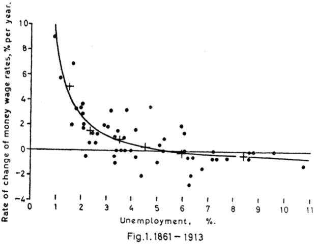
Figure 1: “Original” Phillips curve (Phillips, 1958).

3.2 The Mittag-Leffler Model for Fitting the Phillips Curve

The idea to use a ML-type function to describe the econometric data (representing the Phillips curve) results naturally from observation of two facts:

• the simplicity of the model used by Phillips in his paper (Phillips, 1958) given in (4), where a power-type regression is used to fit the data, where the model can be defined in the form:

  $$y(x)=b\,x^{c}-a,\quad a,b,c\in\mathbb{R},$$ (5)

• the usual shape of the PC, used in the literature, which reminds on the exponential-type function:

  $$y(x)=b\operatorname{e}^{c\,x}-a,\quad a,b,c\in\mathbb{R},$$ (6)

where for both cases, (5) and (6), $x$ stands for the unemployment rate and $y$ for the inflation rate.

Based on these facts, the one-parameter ML function appears to be a general model to fit the PC relation, as it behaves between a purely exponential function and a power function. Some of the possible manifestations of the ML function are shown in Figure 2 (figures generated using the Matlab demo published by Igor Podlubny (Podlubny, 2011)).

(a) $y(x)=c\,E_{\alpha}\,(b\,x^{\alpha}\,)$

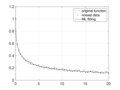
(b) $y(x)=e^{x}\,\operatorname{erfc}\,(\sqrt{x})$

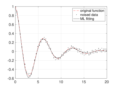
(c) $y(x)=e^{-\alpha x}\cos\,(x)$

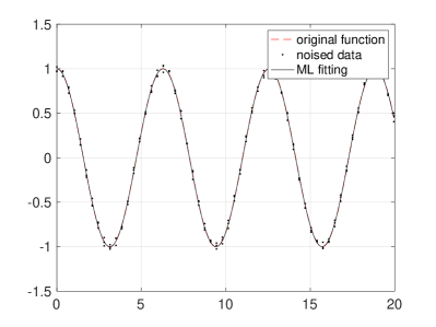
(d) $y(x)=\cos\,(x)$

Figure 2: Mittag-Leffler fitting using different functions $y(x)$ for generating data (Podlubny, 2011).

The one-parameter ML function defined in (1), which includes the special case when $\alpha=1$, i.e. the classical exponential function, is used to model the econometric data under study. Generally, the proposed fitting model can be written as follows:

$$y(x)=c\,E_{\alpha}\,(b\,x^{\alpha}\,),\quad\alpha\in\mathbb{C},\quad\operatorname{Re}(\alpha)>0,\quad b,c\in\mathbb{R},$$ (7)

where the parameters $\alpha,b,c$ are subject to optimisation procedure minimising the squared sum of the vertical offsets between the data points and the fitting curve. For the evaluation of the one-parameter ML function, the Matlab functions created by Podlubny, Chen and Garrappa (Podlubny, 2005, 2011; Chen, 2008a, b; Garrappa, 2015) were used, all giving identical results.

4 Numerical Results and Discussion

To evaluate the performance of the proposed ML model (7) in comparison to the power-type model (5), and the exponential-type model (6) the econometric data of two European countries (France and Switzerland) were used, that were obtained from the EconStats^TM portal (Econstats.com, 2019). The unemployment rate and inflation rate were taken for the period of time 1980-2017. The whole list of the processed data can be found in the Table 3.

4.1 Goodness-of-Fit Statistics and Data Preprocessing

The sum of squared errors (SSE) between the fitting models and the used data serves as the fitting-criterion, with values closer to $0$ indicating a smaller random error component of the model. Also some other quality measures were evaluated, i.e. the R-square from interval $[0,\ 1]$, with values closer to $1$ indicating that a greater proportion of variance is accounted for by the model (e.g. value of $0.7325$ means that the fit explains $73.25\%$ of the total variation in the data about the average); the adjusted R-square statistic, with values smaller or equal to $1$, where values closer to $1$ indicate a better fit; the root mean squared error (RMSE), with values closer to $0$ indicating a fit that is more useful for prediction (MathWorks, 2019).

The used dataset, where the unemployment rate corresponds to the $x$-coordinate and the inflation rate corresponds to the $y$-coordinate of each sample representing the state of these two indicators for each year from the period under study, is first split into two subsets, the “modelling” subset is used to identify the model parameters, the “out-of-sample” subset serves for evaluating the forecast-performance of the models. For both economies, French ad Swiss, all three models were first fitted to the data from the “modelling” subset (composed of 31 samples), by minimising SSE, identifying the optimal parameters. The obtained parameters were then used to compute SSE of the identified models to the “out-of-sample” subset (composed of 7 samples with the greatest values of unemployment rate) and SSE of the fitting model to the complete dataset.

4.2 Experiments

The first experiment was conducted using the French econometric data. The “modelling” subset of 31 samples, was used for the identification purposes. All three models, the power-type model (5), the exponential-type model (6), and the ML model (7), were fitted to these data minimising the SSE obtaining so the optimal parameters. The identified models were then used to compute the SSE to the complete dataset of 38 samples (including the “out-of-sample” subset). SSE results to the “modelling” subset as well as SSE to the “out-of-sample” subset and SSE to the complete dataset for the French Phillips Curve are shown in Table 1, alongside the values of R-square, adjusted R-square, and RMSE. The ML model outperforms the compared models in all listed statistic indicators, with SSE to the “out-of-sample” subset double smaller than the exponential-type model, and almost three-times smaller than the power-type model (see Table 1, where bold stands for better result).

Table 1: The statistical results of the French Phillips curve fitting.

	power-type model	exponential-type model	ML model
SSE to “modelling” subset	157.8422	155.8276	149.6035
SSE to “out-of-sample” subset	10.9024	8.0347	3.9904
SSE to complete dataset	168.7446	163.8623	153.5939
R-square	0.5634	0.569	0.5862
adjusted R-square	0.5322	0.5382	0.5567
RMSE	2.374	2.359	2.311
Model	$y(x)=b\,x^{c}-a$	$y(x)=b\operatorname{e}^{c\,x}-a$	$y(x)=c\,E_{\alpha}\,(b\,x^{\alpha}\,)$
definition
	$a=1.552$	$a=-0.0187$	$\alpha=1.358$
Identified	$b=1.009e+04$	$b=563.6$	$b=-0.6378$
parameters	$c=-3.471$	$c=-0.571$	$c=-149.9$

The result of the French Phillips Curve fitting is also shown in Figure 3, where it is possible to observe a similar behaviour of all three models, i.e. with the increase of the unemployment rate the inflation rate exponentially decreases. However, for the last samples, the decrease of the ML model slows down in comparison to the power-type and exponential-type models. This behaviour of the ML model is obviously better copying the trend of the “out-of-sample” subset. This is also confirmed by the smallest SSE value of the ML fitting curve to the “out-of-sample” subset (see Table 1).

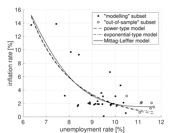
Figure 3: Fitting the French Phillips curve.

Identically as in the French case, the Swiss econometric data (unemployment rate and inflation rate) were first preprocessed. The complete dataset was split into the “modelling” subset composed of 31 samples, that was used to identify the optimal parameters of the power-type model (5), the exponential-type model (6), and the ML model (7). The SSE between the “modelling” subset and the fitting curves was again used as the fitting criterion. Using the identified model parameters the SSE of the evaluated models to the complete dataset of 38 samples (including the “out-of-sample” subset) was computed. In order to compare the forecast-performance of the models SSE to the “out-of-sample” subset, as well as the SSE values for the “modelling” subset fitting, and SSE to the complete dataset for the Swiss Phillips Curve are shown in Table 2, alongside the values of R-square, adjusted R-square, and RMSE.

Table 2: The statistical results of the Swiss Phillips curve fitting.

	power-type model	exponential-type model	ML model
SSE to “modelling” subset	39.6506	40.0588	39.2992
SSE to “out-of-sample” subset	6.8961	4.6826	5.0041
SSE to complete dataset	46.5466	44.7414	44.3033
R-square	0.6389	0.6351	0.642
adjusted R-square	0.6131	0.6091	0.6165
RMSE	1.19	1.196	1.185
Model	$y(x)=b\,x^{c}-a$	$y(x)=b\operatorname{e}^{c\,x}-a$	$y(x)=c\,E_{\alpha}\,(b\,x^{\alpha}\,)$
definition
	$a=-551.3$	$a=-0.7809$	$\alpha=0.7733$
Identified	$b=-548.6$	$b=6.364$	$b=-1.468$
parameters	$c=30.85e-04$	$c=-1.376$	$c=8.823$

Observing the result of the Swiss Phillips Curve fitting shown in Figure 4, one can see an interesting case, where although all the compared models are exponentially decreasing, the curve representing the proposed ML model proceeds in-between the power-type and the exponential-type models, that form a kind of scissors. In respect to the “out-of-sample” subset it is possible to observe that two points of that subset deviate, having higher inflation rate value then the others. This strongly influenced the fitting results. In this case the exponential-type model visually represents the “out-of-sample” subset slightly better then the ML model, that is also demonstrated by a smaller value of SSE of the exponential-type model to the “out-of-sample” subset (see Table 2). In spite of this, the ML model outperforms the compared models in all other used statistic indicators, including smaller SSE to the complete dataset, proving it’s capability. Moreover, in case of filtering these two outliers from the “out-of-sample” subset, the ML model better fits the data-trend.

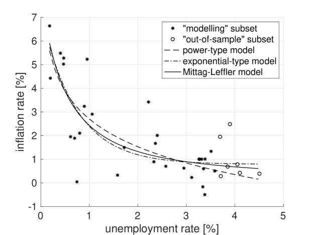
Figure 4: Fitting the Swiss Phillips curve.

5 Conclusion

The ability of the Mittag-Leffler function to behave between the power-type and the exponential-type function, and moreover to fit data that manifest signs of stretched exponentials, oscillations or damped oscillations is demonstrated in this paper, with application to fitting the econometric data (Phillips curve) of two European economies. Exploiting the full potential of the Mittag-Leffler function and it’s generalisations, as well as associating the model parameters with the corresponding economic indicators will be the topic of further work.

The author declare no conflict of interest.

Appendix: The econometric dataset

Table 3: The complete dataset: Econometric data for years 1980 – 2017 (Econstats.com, 2019).

	France		Switzerland
Year	unemployment	inflation	unemployment	inflation
	rate [%]	rate [%]	rate [%]	rate [%]
1980	6.3490	13.7300	0.1970	4.4260
1981	7.4380	13.8900	0.1810	6.6370
1982	8.0690	9.6910	0.4040	5.4850
1983	8.4210	9.2920	0.8010	2.1000
1984	9.7710	6.6900	1.0590	2.9040
1985	10.2300	4.7030	0.8970	3.2380
1986	10.3600	2.1210	0.7440	0.0400
1987	10.5000	3.1150	0.6970	1.8870
1988	10.0100	3.0810	0.6130	1.9490
1989	9.3960	3.5630	0.4690	5.0220
1990	8.9750	3.2120	0.4720	5.2760
1991	9.4670	3.0630	0.9550	5.2270
1992	9.8500	1.9180	2.2190	3.4210
1993	11.1200	2.0700	3.8970	2.4820
1994	11.6800	1.4690	4.1020	0.4200
1995	11.1500	2.1720	3.6950	1.9480
1996	11.5800	2.0860	4.0510	0.7810
1997	11.5400	1.2820	4.5050	0.3860
1998	11.0700	0.6680	3.3380	-0.1680
1999	10.4600	0.5620	2.3620	1.6680
2000	9.0830	1.8270	1.7190	1.4930
2001	8.3920	1.7810	1.5810	0.3250
2002	8.9080	1.9380	2.3300	0.8910
2003	8.9000	2.1690	3.3530	0.5940
2004	9.2330	2.3420	3.5090	1.3320
2005	9.2920	1.9000	3.3840	1.0060
2006	9.2420	1.9120	2.9490	0.6210
2007	8.3670	1.6070	2.4000	2.0040
2008	7.8080	3.1590	2.5760	0.7010
2009	9.5000	0.1030	3.7090	0.2830
2010	9.8020	1.7360	3.8500	0.6860
2011	9.6750	2.2930	3.1100	0.2280
2012	9.9290	1.9520	3.3790	-0.5000
2013	10.0600	1.6300	3.5850	0.5000
2014	9.8010	1.8480	3.3150	1.0000
2015	9.4430	1.9040	3.2780	1.0000
2016	9.1440	1.9490	3.2590	1.0000
2017	8.8350	2.0150	3.2620	1.0000

References

- Samuelson and Solow (1960) Samuelson, P.A.; Solow, R.M. Analytical aspects of anti-inflation policy. American Economic Review 1960, 50, 177–194.
- Phillips (1958) Phillips, A.W. The relation between unemployment and the rate of change of money wage rates in the United Kingdom, 1861-1957. Economica 1958, 25, 283–299.
- Fisher (1926) Fisher, I. A Statistical Relation between Unemployment and Price Changes. International Labour Review 1926, 13, 785Ж792. Reprinted as 1973, I Discovered the Phillips Curve: A Statistical Relation between Unemployment and Price Changes, Journal of Political Economy, 81(2, Part 1), pp. 496–502.
- Brown (1955) Brown, A.J. Great Inflation 1939-1951; Oxford University Press, London, 1955.
- Lipsey (1960) Lipsey, R.G. The relation between unemployment and the rate of change of money wage rates in the United Kingdom, 1862-1957: A further analysis. Economica 1960, 27, 1–31.
- Bowen (1960) Bowen, W.G. Wage Behavior in the Postwar Period: An Empirical Analysis; Princeton, 1960.
- Bodkin (1966) Bodkin, R.G. The Wage-Price-Productivity Nexus; Philadelphia, 1966.
- Taylor (1979) Taylor, J.B. Staggered Wage Setting in a Macro Model. American Economic Review 1979, 69, 108–113.
- Taylor (1980) Taylor, J.B. Aggregate dynamics and staggered contracts. Journal of Political Economy 1980, 88, 1–23.
- Calvo (1983) Calvo, G.A. Staggered Prices In A Utility-maximizing Framework. Journal of Monetary Economics 1983, 12, 383–398.
- Rotemberg (1982) Rotemberg, J.J. Monopolistic Price Adjustment and Aggregate Output. Review of Economic Studies 1982, 49, 517–531.
- Rotemberg and Woodford (1997) Rotemberg, J.J.; Woodford, M. An Optimization-Based Econometric Framework for the Evaluation of Monetary Policy. NBER Macroeconomics Annual, Cambridge, MA: MIT Press 1997, pp. 297–346.
- Friedman (1968) Friedman, M. The role of monetary policy. American Economic Review 1968, 58, 1–17.
- Phelps (1968) Phelps, E.S. Money-Wage Dynamics and Labor Market Equilibrium. Journal of Political Economy 1968, 76, 678–711.
- Clarida et al. (1999) Clarida, R.; Galí, J.; Gertler, M. The science of monetary policy: A new Keynesian perspective. Journal of Economic Literature 1999, 37, 1661–1707.
- McCallum (1997) McCallum, B.T. Comment. NBER Macroeconomics Annual, Cambridge, MA: MIT Press 1997, 12, 355–359.
- Galí and Gertler (1999) Galí, J.; Gertler, M. Inflation Dynamics: A Structural Econometric Analysis. Journal of Monetary Economics 1999, 44, 195–222.
- Galí et al. (2001) Galí, J.; Gertler, M.; López-Salido, J.D. European Inflation Dynamics. European Economic Review 2001, 45, 1237–1270.
- Galí et al. (2005) Galí, J.; Gertler, M.; López-Salido, J.D. Robustness of the Estimates of the Hybrid New Keynesian Phillips Curve. Journal of Monetary Economics 2005, 52, 1107–1118.
- Mittag-Leffler (1903a) Mittag-Leffler, M.G. Sur la nouvelle fonction . Comptes Rendus de l’Académie des Sciences 1903, 137, 554–558.
- Mittag-Leffler (1903b) Mittag-Leffler, M.G. Une generalisation de l’integrale de Laplace-Abel. Comptes Rendus de l’Académie des Sciences 1903, 137, 537–539.
- Hille and Tamarkin (1930) Hille, E.; Tamarkin, J.D. On the theory of linear integral equations. Annals of Mathematics 1930, 31, 479–528.
- Dzhrbashyan (1966) Dzhrbashyan, M.M. Integral Transforms and Representations of Functions in Complex Plane; Nauka, Moscow, Russia, 1966.
- Caputo and Mainardi (1971) Caputo, M.; Mainardi, F. Linear models of dissipation in anelastic solids. La Rivista del Nuovo Cimento 1971, 1, 161–198.
- Blair (1974) Blair, G.W.S. Psychorheology: links between the past and the present. Journal of Texture Studies 1974, 5, 3–12.
- Torvik and Bagley (1984) Torvik, P.J.; Bagley, R.L. On the appearance of the fractional derivative in the behaviour of real materials. Journal of Applied Mechanics 1984, 51, 294–298.
- Samko et al. (1993) Samko, S.G.; Kilbas, A.A.; Marichev, O.I. Fractional Integrals and Derivatives: Theory and Applications; Gordon and Breach, New York, NY, USA, 1993.
- Gorenflo and Vessella (1991) Gorenflo, R.; Vessella, S. Abel Integral Equations: Analysis and Applications; Lecture Notes in Mathematics, Springer, Berlin, Germany, 1991; pp. –.
- Gorenflo and Mainardi (1996) Gorenflo, R.; Mainardi, F. Fractional Oscillations and Mittag-Leffler Functions. Technical Report 1- 14/96, Free University of Berlin, Berlin, Germany, 1996.
- Gorenflo and Mainardi (1997) Gorenflo, R.; Mainardi, F., Fractals and Fractional Calculus in Continuum Mechanics; Springer, Berlin, Germany, 1997; chapter Fractional calculus: Integral and differential equations of fractional order, pp. 223–276.
- Gorenflo et al. (2002) Gorenflo, R.; Loutchko, J.; Luchko, Y. Computation of the Mittag-Leffler function and its derivatives. Fractional Calculus & Applied Analisys 2002, 5, 491–518.
- Gorenflo et al. (2014) Gorenflo, R.; Kilbas, A.A.; Mainardi, F.; Rogosin, S.V. Mittag-Leffler Functions, Related Topics and Applications; Springer Monographs in Mathematics, Springer-Verlag, Berlin Heidelberg, 2014.
- Kilbas and Saigo (1995) Kilbas, A.A.; Saigo, M. On solutions of integral equations of Abel-Volterra type. Differential and Integral Equations 1995, 8, 993–1011.
- Kilbas and Saigo (1996) Kilbas, A.A.; Saigo, M. On Mittag-Leffler type function, fractional calculus operators and solutions of integral equations. Integral Transforms and Special Functions 1996, 4, 355–370.
- Kilbas et al. (2004) Kilbas, A.A.; Saigo, M.; Saxena, R.K. Generalized Mittag-Leffler function and generalized fractional calculus operators. Integral Transforms and Special Functions 2004, 15, 31–49.
- Mainardi and Gorenflo (1996) Mainardi, F.; Gorenflo, R., Boundary Value Problems, Special Functions and Fractional Calculus. In Boundary Value Problems, Special Functions and Fractional Calculus; Kilbas, A.A., Ed.; Byelorussian State University, Minsk, Belarus, 1996; chapter The Mittag-Leffler function in the Riemann-Liouville fractional calculus, pp. 215–225.
- Mainardi and Gorenflo (2000) Mainardi, F.; Gorenflo, R. On Mittag-Leffler-type functions in fractional evolution processes. Journal of Computational and Applied Mathematics 2000, 118, 283–299.
- Srivastava and Saxena (2001) Srivastava, H.M.; Saxena, R.K. Operators of fractional integration and their applications. Applied Mathematics and Computation 2001, 118, 1–52.
- Srivastava and Tomovski (2009) Srivastava, H.M.; Tomovski, Z. Fractional calculus with an integral operator containing a generalized Mittag-Leffler function in the kernel. Applied Mathematics and Computation 2009, 211, 198–210.
- West et al. (2003) West, B.; Mauro Bologna, M.; Grigolini, P. Physics of fractal operators; Springer-Verlag, New York, 2003.
- Haubold et al. (2011) Haubold, H.J.; Mathai, A.M.; Saxena, R.K. Mittag-Leffler functions and their applications. Journal of Applied Mathematics 2011, 2011, 51. Article ID 298628
- Garrappa (2015) Garrappa, R. Numerical evaluation of two and three parameter Mittag-Leffler functions. SIAM Journal of Numerical Analysis 2015, 53, 1350–1369.
- Chen (2008a) Chen, Y. Generalized Mittag-Leffler function; MathWorks, Inc. Matlab Central File Exchange, url: http://www.mathworks.com/matlabcentral/fileexchange/20849, 2008.
- Chen (2008b) Chen, Y. Generalized Generalized Mittag-Leffler function; MathWorks, Inc. Matlab Central File Exchange, url: http://www.mathworks.com/matlabcentral/fileexchange/21454, 2008.
- Podlubny (2005) Podlubny, I. Mittag-Leffler function; MathWorks, Inc. Matlab Central File Exchange, url: http://www.mathworks.com/matlabcentral/fileexchange/8738, 2005.
- Podlubny (2011) Podlubny, I. Fitting data using the Mittag-Leffler function; MathWorks, Inc. Matlab Central File Exchange, url: http://www.mathworks.com/matlabcentral/fileexchange/32170, 2011.
- Garrappa (2015) Garrappa, R. The Mittag-Leffler function; MathWorks, Inc. Matlab Central File Exchange, url: http://www.mathworks.com/matlabcentral/fileexchange/48154, 2015.
- Matychyn (2017) Matychyn, I. Matrix Mittag-Leffler Function; MathWorks, Inc. Matlab Central File Exchange, url: http://www.mathworks.com/matlabcentral/fileexchange/62790, 2017.
- Capelas de Oliveira et al. (2011) Capelas de Oliveira, E.; Mainardi, F.; Vaz Jr., J. Models based on Mittag-Leffler functions for anomalous relaxation in dielectrics. The European Physical Journal Special Topics 2011, 193, 161–171.
- Petras et al. (2012) Petras, I.; Sierociuk, D.; Podlubny, I. Identification of Parameters of a Half-Order System. IEEE Transactions on Signal Processing 2012, 60, 5561–5566.
- Sierociuk et al. (2013) Sierociuk, D.; Podlubny, I.; Petras, I. Experimental Evidence of Variable-Order Behavior of Ladders and Nested Ladders. IEEE Transactions on Control Systems Technology 2013, 21, 459–466.
- Maindardi (2018) Maindardi, F. Fractional Calculus and Waves in Linear Vescoelasticity: An Introduction to Mathematical Models (Second Revised Edition); Imperial College Press, 2018.
- Samuel et al. (2016) Samuel, S.; Ricon, J.; Podlubny, I. Modelling combustion in internal combustion engines using the Mittag-Leffler function. ICFDA 16: International Conference on Fractional Differentiation and its Applications, Novi Sad, Serbia, July 18 - 20, 2016, 2016, pp. 551–552.
- Zeng et al. (2015) Zeng, C.; Chen, Y.; Podlubny, I. Is our universe accelerating dynamics fractional order? 2015 ASME/IEEE International Conference on Mechatronic and Embedded Systems and Applications, Boston, Aug. 2-5, 2015, 2015. Paper No. DETC2015-46216.
- Scalas et al. (2000) Scalas, E.; Gorenflo, R.; Mainardi, F. Fractional calculus and continuous-time finance. Physica A: Statistical Mechanics and its Applications 2000, 284, 376–384.
- Gorenflo et al. (2001) Gorenflo, R.; Mainardi, F.; Scalas, E.; Raberto, M. Fractional Calculus and Continuous-Time Finance III : the Diffusion Limit. In Mathematical Finance: Workshop of the Mathematical Finance Research Project, Konstanz, Germany, October 5-7, 2000; Birkhauser Basel: Basel, 2001; pp. 171–180.
- Mainardi et al. (2000) Mainardi, F.; Raberto, M.; Gorenflo, R.; Scalas, E. Fractional calculus and continuous-time finance II: The waiting-time distribution. Physica A: Statistical Mechanics and its Applications 2000, 287, 468–481.
- Mainardi et al. (2002) Mainardi, F.; Raberto, M.; Scalas, E.; Gorenflo, R. Empirical Science of Financial Fluctuations - The Advent of Econophysics; Springer Japan, 2002; chapter Survival probability of LIFFE bond futures via the Mittag-Leffler function, pp. 195 – 206.
- Cartea and del Castillo-Negrete (2007) Cartea, ç.; del Castillo-Negrete, D. Fractional diffusion models of option prices in markets with jumps. Physica A: Statistical Mechanics and its Applications 2007, 374, 749–763.
- Vilela Mendes (2008) Vilela Mendes, R. A fractional calculus interpretation of the fractional volatility model. Nonlinear Dynamics 2008, 55, 395.
- Garibaldi and Scalas (2010) Garibaldi, U.; Scalas, E. Finitary Probabilistic Methods in Econophysics; Cambridge University Press, 2010.
- Skovranek et al. (2012) Skovranek, T.; Podlubny, I.; Petras, I. Modeling of the national economies in state-space: A fractional calculus approach. Economic Modelling 2012, 29, 1322–1327.
- Tejado (2015) Tejado, I.; Valerio, D.; Perez, E.; Valerio, N. Fractional calculus in economic growth modelling: The Spanish and Portuguese cases. Int. J. Dyn. Control 2015, 5, 208–222.
- Tejado (2018) Tejado, I.; Perez, E.; Valerio, D. Fractional calculus in economic growth modelling of the group of seven. SSRN Electron. J. 2018.
- Tarasov (2016) Tarasov, V.E.; Tarasova, V.V. Long and short memory in economics: Fractional-order difference and differentiation. IRA Int. J. Manag. Soc. Sci. 2016, 5, 327–334.
- Tarasov and Tarasova (2017) Tarasov, V.E.; Tarasova, V.V. Time-dependent fractional dynamics with memory in quantum and economic physics. Annals of Physics 2017, 383, 579–599.
- Tarasova and Tarasov (2018) Tarasova, V.V.; Tarasov, V.E. Concept of dynamic memory in economics. Communications in Nonlinear Science and Numerical Simulation 2018, 55, 127–145.
- Tarasov (2018) Tarasov, V.E.; Tarasova, V.V. Macroeconomic models with long dynamic memory: Fractional calculus approach. Appl. Math. Comput. 2018, 338, 466–486.
- Tarasov (2019) Tarasov, V.E. Economic models with power-law memory. In Handbook of Fractional Calculus with Applications; Volume 8: Applications in Engineering, Life and Social Sciences, Part B; Chapter 1; De Gruyter: Berlin, Germany, 2019; ISBN 978-3-11-057092-2.
- Tarasov (2019a) Tarasov, V.E.; Tarasova, V.V. Phillips model with exponentially distributed lag and power-law memory. Comput. Appl. Math. 2019, 38, 13.
- Tarasov (2019b) Tarasov, V.E.; Tarasova, V.V. Harrod-Domar growth model with memory and distributed lag. Axioms 2019, 8, 9.
- Tarasov (2019c) Tarasov, V.E.; Tarasova, V.V. Dynamic Keynesian Model of Economic Growth with Memory and Lag. Mathematics 2019, 7,178, 17.
- Econstats.com (2019) Econstats.com. EconStats : World Economic Outlook (WEO) data, IMF. [online] Available at: http://www.econstats.com [Accessed 21 May 2019], 2019.
- Erdélyi et al. (1955) Erdélyi, A.; Magnus, W.; Oberhettinger, F.; Tricomi, F.G. Higher Transcendental Functions; Vol. 3, McGraw-Hill, New York, NY, USA, 1955; pp. –.
- Mittag-Leffler (1904) Mittag-Leffler, M.G. Sopra la funzione . Comptes Rendus de l’Académie des Sciences 1904, 13, 3–5.
- Mittag-Leffler (1905) Mittag-Leffler, M.G. Sur la représentation analytique d’une branche uniforme d’une fonction monogène - cinquième note. Acta Mathematica 1905, 29, 101–181.
- Wiman (1905a) Wiman, A. Über den Fundamentalsatz in der Teorie der Funktionen . Acta Mathematica 1905, 29, 191–201.
- Wiman (1905b) Wiman, A. Über die Nullstellen der Funktionen . Acta Mathematica 1905, 29, 217–234.
- Pollard (1948) Pollard, H. The completely monotonic character of the Mittag-Leffler function . Bulletin of the American Mathematical Society 1948, 54, 1115–1116.
- Agarwal (1953) Agarwal, R.P. A propos d’une note de M. Pierre Humbert. Comptes Rendus de l’Académie des Sciences 1953, 236, 2031–2032.
- Humbert (1953) Humbert, P. Quelques résultats relatifs à la fonction de Mittag-Leffler. Comptes Rendus de l’Académie des Sciences Paris 1953, 236, 1467–1468.
- Humbert and Agarwal (1953) Humbert, P.; Agarwal, R.P. Sur la fonction de Mittag-Leffler et quelques-unes de ses généralisations. Bulletin des Sciences Mathématiques 1953, 77, 180–185.
- Prabhakar (1971) Prabhakar, T.R. A singular integral equation with a generalized Mittag-Leffler function in the kernel. Yokohama Mathematical Journal 1971, 19, 7–15.
- Rainville (1960) Rainville, E.D. Special Functions; Macmillan, New York USA, 1960.
- Shukla and Prajapati (2007) Shukla, A.K.; Prajapati, J.C. On a generalization of Mittag-Leffler function and its properties. Journal of Mathematical Analysis and Applications 2007, 336, 797–811.
- Cover (1992) Cover, J.P. Asymmetric effects of positive and negative money-supply shocks. Quarterly Journal of Economics 1992, 107, 1261–1282.
- Karras (1996) Karras, G. Are the output effects of monetary policy asymmetric? Evidence from a sample of European countries. Oxford Bulletin of Economics and Statistics 1996, 58, 267–278.
- Nobay and Peel (2000) Nobay, A.R.; Peel, D.A. Optimal monetary policy with a nonlinear Phillips curve. Economics Letters 2000, 67, 159–164.
- Schaling (2004) Schaling, E. The nonlinear Phillips curve and inflation forecast targeting: Symmetric versus asymmetric monetary policy rules. Journal of Money, Credit and Banking 2004, 36, 361–386.
- Stiglitz (1997) Stiglitz, J. Reflections on the natural rate hypothesis. Journal of Economic Perspectives 1997, 11, 3–10.
- Filardo (1998) Filardo, A. New evidence on the output cost of fighting inflation. Federal Reserve Bank of Kansas City Economic Review 1998, 83, 33–61.
- Brown and Hopkins (1950) Brown, P.; Hopkins, S. The Course of Wage-Rates in Five Countries, 1860-1939. Oxford Economic Papers 1950, II.
- MathWorks (2019) MathWorks, Inc. Evaluating Goodness of Fit. [online] Available at: https://www.mathworks.com/help/curvefit/evaluating-goodness-of-fit.html [Accessed 21 May 2019], 2019.