High order implicit time integration schemes on multiresolution adaptive grids for stiff PDE’s

Abstract

We consider high order, implicit Runge–Kutta schemes to solve time–dependent stiff PDEs on dynamically adapted grids generated by multiresolution analysis for unsteady problems disclosing localized fronts. The multiresolution finite volume scheme yields highly compressed representations within a user–defined accuracy tolerance, hence strong reductions of computational requirements to solve large, coupled nonlinear systems of equations. SDIRK and RadauIIA Runge–Kutta schemes are implemented with particular interest in those with $L-$stability properties and accuracy–based time–stepping capabilities. Numerical evidence is provided of the computational efficiency of the numerical strategy to cope with highly unsteady problems modeling various physical scenarios with a broad spectrum of time and space scales.

Keywords: High order time discretization, multiresolution finite volume scheme, stiff PDEs, implicit Runge–Kutta schemes, error control.

AMS subject classifications: 65M50, 65M08, 65G20, 65L04, 65L06, 65M20.

1 Introduction

In many scientific applications, from biomedical models to combustion or air pollution modeling, stiff differential equations must be solved to carry out numerical simulations. A straightforward notion of stiffness was given by Hairer & Wanner by stating that stiff equations are problems for which explicit methods don’t work [34]. The latter is mainly due to the broad spectrum of physical or numerical time scales that a numerical solver must deal with whenever a stiff time–dependent differential equation is being solved. Robust and stable methods are thus required for stiff problems in order to properly handle and damp out fast transients. In the past decades high order implicit Runge–Kutta schemes with excellent stability properties were developed and widely investigated to solve stiff problems modeled by ODEs (see [34] § IV and references therein). The same methods can be naturally considered to solve stiff problems originating from time–dependent PDEs discretized in space. However, the high performance of implicit Runge–Kutta methods for stiff ODEs is often adversely affected by the size of the systems of nonlinear equations arising in the case of semi–discrete PDEs. In particular phenomena involving localized fronts, as considered in this work, commonly require fine spatial representations, hence potentially large systems of equations. Significant effort is required to achieve numerical implementations that solve the corresponding algebraic problems at reasonable computational expenses in terms of both CPU time and memory.

Low order implicit schemes were already successfully used to simulate very complex problems modeled by stiff PDEs. This is the case, for instance, for the numerical simulation of combustion flames accounting for detailed chemical kinetics and multi–species transport (see, e.g., [4, 49] and references therein). The computational performance of high order Runge–Kutta methods, implemented in well–established production aerodynamics codes, was also assessed in the context of laminar and turbulent compressible flows [9, 14]. In particular Jacobian–free Newton–Krylov methods were investigated in conjunction with high order implicit schemes [38, 8] to further reduce the computational requirements (see, e.g., [39] for a review on this subject). Similarly, high order space discretization schemes have also been implemented in this context, reducing in practice the computational stencils, hence the size of the nonlinear systems [43, 42]. Easing the computational load is also achievable by designing efficient parallelization techniques as developed, for instance, in [51] for reactive flow solvers. Taking into account that grid adaptation techniques for unsteady problems disclosing localized fronts are specifically designed to yield high data compression, we exploit this capability here to efficiently implement implicit integration schemes for stiff PDEs. This strategy was already adopted, for instance, in [5, 6], together with low order implicit solvers.

Among the many adaptive meshing approaches developed in the literature, we consider in this work adaptive multiresolution schemes based on [35, 36], namely the multiresolution finite volume scheme introduced in [17] for conservation laws. Besides the inherent advantages of grid adaptation, multiresolution techniques rely on biorthogonal wavelet decomposition and thus offer a rigorous mathematical framework for adaptive meshing schemes [16, 41]. Consequently, not only approximation errors coming from grid adaptation can be tracked, but general and robust solvers can be implemented since the wavelet decomposition is independent of any physical particularity of the problem and accounts only for the spatial regularity of the discrete variables at a given simulation time. Adaptive multiresolution schemes have been successfully implemented for the simulation of compressible fluids (see, e.g., [10, 19] and references therein), as well as for the numerical solution of time–dependent, parabolic [46, 11] and stiff parabolic [24, 25] PDEs. Nevertheless, to the best of our knowledge this is the fist attempt to implement high order implicit time integration schemes in the context of the adaptive multiresolution finite volume method to solve stiff PDEs.

The paper is organized as follows. We give in Section 2 a short introduction on multiresolution finite volume schemes and implicit Runge–Kutta schemes, in particular of SDIRK– (Singly Diagonally Implicit Runge–Kutta) and RadauIIA– type. Some key aspects of the numerical implementation of time implicit schemes on multiresolution grids are detailed in Section 3. Finally, the numerical solution of several stiff time–dependent PDEs is investigated in Section 4.

2 Numerical methodology

Let us consider a parabolic, time–dependent PDE,

$$\left.\begin{array}[]{ll}\partial_{t}{\boldsymbol{u}}={\boldsymbol{F}}(\partial^{2}_{{\boldsymbol{x}}}{\boldsymbol{u}},\partial_{{\boldsymbol{x}}}{\boldsymbol{u}},{\boldsymbol{u}}),&t>t_{0},\,{\boldsymbol{x}}\in{\mathbb{R}}^{d},\\ {\boldsymbol{u}}(t_{0},{\boldsymbol{x}})={\boldsymbol{u}}_{0}({\boldsymbol{x}}),&t=t_{0},\,{\boldsymbol{x}}\in{\mathbb{R}}^{d},\end{array}\right\}$$ (1)

where ${\boldsymbol{u}}:{\mathbb{R}}\times{\mathbb{R}}^{d}\to{\mathbb{R}}^{m}$ and ${\boldsymbol{F}}:{\mathbb{R}}^{m}\to{\mathbb{R}}^{m}$, for a model with $m$ variables. For many physically inspired systems, the right hand side ${\boldsymbol{F}}$ can in general be written as

$${\boldsymbol{F}}(\partial^{2}_{{\boldsymbol{x}}}{\boldsymbol{u}},\partial_{{\boldsymbol{x}}}{\boldsymbol{u}},{\boldsymbol{u}})={\boldsymbol{F}}({\boldsymbol{u}})={\boldsymbol{F}}_{1}({\boldsymbol{u}})+{\boldsymbol{F}}_{2}({\boldsymbol{u}})+\ldots,$$ (2)

where the ${\boldsymbol{F}}_{i}({\boldsymbol{u}})$, $i=1,\ldots$, stand for different physical processes. For instance, a scalar nonlinear reaction–diffusion equation with $u:{\mathbb{R}}\times{\mathbb{R}}^{d}\to{\mathbb{R}}$ would be given by $F_{1}(u)=-\partial_{{\boldsymbol{x}}}\cdot(D(u)\partial_{{\boldsymbol{x}}}u)$ and $F_{2}(u)=f(u)$ for some diffusion coefficient, $D:{\mathbb{R}}\to{\mathbb{R}}$, and a nonlinear function, $f:{\mathbb{R}}\to{\mathbb{R}}$.

2.1 Multiresolution analysis

Without loss of generality we perform a finite volume discretization of problem (1) with $m=1$ for the sake of simplicity. According to the multiresolution finite volume scheme [17], we consider a set of nested dyadic grids over a computational domain $\Omega\subset\mathbb{R}^{d}$ as follows. Each cell $\Omega_{\lambda}$, $\lambda\in S_{j}$, is the union of $2^{d}$ finer cells of equal size $\Omega_{\mu}$, $\mu\in S_{j+1}$. The sets $S_{j}$ and $S_{j+1}$ are thus consecutive embedded grids over $\Omega$, where $j=0,1,\ldots,J$, corresponds to the grid–level, from the coarsest to the finest grid, i.e., $j$ equal to 0 and $J$, respectively. We denote ${\mathbf{U}}_{j}:=(u_{\lambda})_{\lambda\in S_{j}}$ as the spatial representation of $u$ on the grid $S_{j}$, where $u_{\lambda}$ represents the cell–average of $u:\,{\mathbb{R}}\times{\mathbb{R}}^{d}\to{\mathbb{R}}$ in $\Omega_{\lambda}$:

$$u_{\lambda}:=|\Omega_{\lambda}|^{-1}\int_{\Omega_{\lambda}}u(t,{\boldsymbol{x}})\,{\mathrm{d}}{\boldsymbol{x}},\quad{\boldsymbol{x}}\in{\mathbb{R}}^{d}.$$ (3)

Data at different levels of discretization are related by two inter–level transformations: the projection and prediction operators, briefly defined in Appendix A. Based on these operations, a multiresolution analysis allows one to define a one–to–one correspondence between two consecutive grid–levels:

$${\mathbf{U}}_{j}\longleftrightarrow({\mathbf{U}}_{j-1},{\mathbf{D}}_{j}),$$ (4)

where the ${\mathbf{D}}_{j}$ array gathers the so–called details. The latter can be seen as estimators of the local spatial regularity of a given discretized function, in this case ${\mathbf{U}}_{j}$, and represent the information lost when coarsening the spatial grid, in this case from ${\mathbf{U}}_{j}$ to ${\mathbf{U}}_{j-1}$. By iteration of this decomposition, we get a multi–scale representation of ${\mathbf{U}}_{J}$ in terms of ${\mathbf{M}}_{J}:=({\mathbf{U}}_{0},{\mathbf{D}}_{1},{\mathbf{D}}_{2},\cdots,{\mathbf{D}}_{J})$:

$${\mathcal{M}}:{\mathbf{U}}_{J}\longmapsto{\mathbf{M}}_{J},$$ (5)

and similarly, its inverse ${\mathcal{M}}^{-1}$. This multi–scale transform amounts to a representation of ${\mathbf{U}}_{J}$ in a wavelet space spanned by a biorthogonal wavelet basis. Further details can be found in [16, 41].

While the transformation (5) is exact and the multi–scale representation can be performed back and forth, real computational benefit is achieved by introducing a thresholding operator, as shown in Appendix A. This operator basically discards cells of smooth regularity whose values can be recomputed within an accuracy tolerance whenever needed. As a result a multiresolution approximation ${\mathbf{U}}_{J}^{\epsilon}$ is obtained. Defining the following normalized $\ell^{2}$–norm:

$$\|{\mathbf{U}}_{J}\|_{2}^{2}:=2^{-dJ}\displaystyle\sum_{\lambda\in S_{J}}(u_{\lambda})^{2},$$

which corresponds to the $L^{2}$–norm of a piecewise constant function, it can be shown that [21]

$$\|{\mathbf{U}}_{J}-{\mathbf{U}}_{J}^{\epsilon}\|_{2}\leq C{\eta_{\mathrm{MR}}},$$ (6)

where ${\eta_{\mathrm{MR}}}$ corresponds to an accuracy tolerance.

So much is true for steady problems. When solving time–dependent problems, the same behavior is expected in terms of numerical errors introduced by the multiresolution approximation. (The spatially adapted grid is fixed during a given time integration step.) The latter was mathematically proved for hyperbolic problems in an $L^{1}$–norm for both classical and inhomogeneous conservation laws in [17] and [37], respectively. Moreover, numerical evidence proves similar behaviors for time–dependent, parabolic [46, 11, 3] and stiff parabolic [24, 22, 23] PDEs.

2.2 Implicit Runge–Kutta schemes

Let us now consider problem (1) discretized on an adapted grid obtained by multiresolution analysis:

$$\left.\begin{array}[]{ll}{\mathrm{d}}_{t}{\mathbf{U}}={\mathbf{F}}({\mathbf{U}}),&t>t_{0},\\ {\mathbf{U}}(t_{0})={\mathbf{U}}_{0},&t=t_{0}.\end{array}\right\}$$ (7)

For the ease of reading we denote ${\mathbf{U}}_{J}^{\epsilon}$ simply as ${\mathbf{U}}$ of size $m\times N$, where $N$ corresponds to the number of cells in the adapted grid and thus ${\mathbf{F}}:{\mathbb{R}}^{m\times N}\to{\mathbb{R}}^{m\times N}$.

Given a time step $\Delta t$ we consider an implicit Runge–Kutta (IRK) scheme of order $p$ for the numerical integration of the semi–discretized problem (7). An $s$–stage Runge–Kutta scheme is in general defined through a set of arrays ${\boldsymbol{b}}$, ${\boldsymbol{c}}\in{\mathbb{R}}^{s}$, such that ${\boldsymbol{b}}=(b_{1},\ldots,b_{s})^{T}$ and ${\boldsymbol{c}}=(c_{1},\ldots,c_{s})^{T}$, and a matrix ${\boldsymbol{A}}\in\mathcal{M}_{s}({\mathbb{R}})$ such that ${\boldsymbol{A}}=(a_{ij})_{1\leq i,j\leq s}$. These coefficients define the stability properties and the order conditions of the method, and are usually arranged in a Butcher tableau according to

$$\begin{tabular}[]{c|c }${\boldsymbol{c}}$&${\boldsymbol{A}}$\\ \hline\cr\\[-10.76385pt] &${\boldsymbol{b}}^{T}$\end{tabular}.$$

In practice, given a set of arrays ${\mathbf{z}}_{1},\ldots,{\mathbf{z}}_{s}\in{\mathbb{R}}^{m\times N}$, we have to solve the nonlinear system

$$\left(\begin{array}[]{c}{\mathbf{z}}_{1}\\ \vdots\\ {\mathbf{z}}_{s}\end{array}\right)={\mathbf{A}}\left(\begin{array}[]{c}\Delta t{\mathbf{F}}(t_{0}+c_{1}\Delta t,{\mathbf{U}}_{0}+{\mathbf{z}}_{1})\\ \vdots\\ \Delta t{\mathbf{F}}(t_{0}+c_{s}\Delta t,{\mathbf{U}}_{0}+{\mathbf{z}}_{s})\end{array}\right),$$ (8)

where ${\mathbf{A}}$ is a square block–matrix of size $s\times m\times N$ built with the coefficients $(a_{ij})_{1\leq i,j\leq s}$ (see more details in Appendix B). The solution ${\mathbf{U}}(t_{0}+\Delta t)$ is then approximated by ${\mathbf{U}}_{1}$, computed as

$${\mathbf{U}}_{1}={\mathbf{U}}_{0}+\displaystyle\sum_{i=1}^{s}d_{i}{\mathbf{z}}_{i},\qquad{\boldsymbol{d}}^{T}:=(d_{1},\ldots,d_{s})=(b_{1},\ldots,b_{s}){\boldsymbol{A}}^{-1}.$$ (9)

If all the elements of the matrix of coefficients ${\boldsymbol{A}}$ are non–zero, then we say we are considering a fully IRK scheme [34]. Moreover, if

$$a_{sj}=b_{j},\quad j=1,\ldots,s$$ (10)

then the last stage corresponds to the solution ${\mathbf{U}}_{1}$ and thus ${\boldsymbol{d}}^{T}=(0,0,\ldots,0,1)$ in (9). Methods satisfying (10) are called stiffly accurate [44] and are particularly appropriate for the solution of (stiff) singular perturbation problems and for differential–algebraic equations [32, 34].

An IRK approximation amounts then to solving a nonlinear system of equations of size $s\times m\times N$. The latter can be achieved by considering a simplified Newton method for system (8), recast as

$${\boldsymbol{\mathcal{G}}}({\mathbf{Z}}):={\mathbf{Z}}-\Delta t{\mathbf{A}}{\boldsymbol{\mathcal{F}}}({\mathbf{Z}})={\mathbf{0}},$$ (11)

where ${\mathbf{Z}}:=({\mathbf{z}}_{1},\ldots,{\mathbf{z}}_{s})^{T}$ and ${\boldsymbol{\mathcal{F}}}({\mathbf{Z}}):=({\mathbf{F}}(t_{0}+c_{1}\Delta t,{\mathbf{U}}_{0}+{\mathbf{z}}_{1}),\ldots,{\mathbf{F}}(t_{0}+c_{s}\Delta t,{\mathbf{U}}_{0}+{\mathbf{z}}_{s}))^{T}$. The $(k+1)$–th approximation of the solution ${\mathbf{Z}}$ is thus computed in two steps. First, we solve the following linear system for $\delta{\mathbf{Z}}^{k}\in{\mathbb{R}}^{s\times m\times N}$:

$$({\mathbf{Id}}_{s\times m\times N}-\Delta t{\mathbf{A}}{\mathbf{J}})\delta{\mathbf{Z}}^{k}=-{\mathbf{Z}}^{k}+\Delta t{\mathbf{A}}{\boldsymbol{\mathcal{F}}}({\mathbf{Z}}^{k}),$$ (12)

where ${\mathbf{J}}$ is a a square block–matrix of size $s\times m\times N$ consisting of $s$ rows and $s$ columns of size $m\times N$ given by the Jacobians ${\mathbf{J}}_{0}:=\partial_{{\mathbf{U}}}{\mathbf{F}}(t_{0},{\mathbf{U}}_{0})$. Then, the previous solution ${\mathbf{Z}}^{k}$ is corrected according to

$${\mathbf{Z}}^{k+1}={\mathbf{Z}}^{k}+\delta{\mathbf{Z}}^{k}.$$ (13)

A standard way of initializing the iterative algorithm considers simply

$${\mathbf{z}}_{i}^{0}={\mathbf{U}}_{0},\quad i=1,\ldots,s.$$ (14)

2.2.1 SDIRK schemes

An alternative to solving a large nonlinear system of size $s\times m\times N$ is to consider an SDIRK scheme where $a_{ij}=0$ for $j>i$, and with equal diagonal coefficients, i.e., $a_{ii}=\gamma$, $i=1,\ldots,s$. In general, $A$– or $L$–stable SDIRK schemes can be built of order $p\leq s+1$ or $p\leq s$, respectively (see [34] § IV.6 for more details). However, the stage order $q$ of these schemes, that is, the order achieved by one single stage, is limited to $1$.

The main idea is thus to successively solve the $s$ stages by considering an $m\times N$–dimensional system at each stage, that is, for $i=1,\ldots,s$,

$${\mathbf{z}}_{i}=\Delta t\gamma{\mathbf{F}}(t_{0}+c_{i}\Delta t,{\mathbf{U}}_{0}+{\mathbf{z}}_{i})+\Delta t\displaystyle\sum_{j=1}^{i-1}a_{ij}{\mathbf{F}}(t_{0}+c_{j}\Delta t,{\mathbf{U}}_{0}+{\mathbf{z}}_{j}),$$ (15)

where the second term in the right–hand side is already known at the current stage. Adopting the same simplified Newton technique, this time stage–wise, we have to solve the following linear system for $\delta{\mathbf{z}}_{i}^{k}\in{\mathbb{R}}^{m\times N}$:

$$({\mathbf{Id}}_{m\times N}-\Delta t\gamma{\mathbf{J}}_{0})\delta{\mathbf{z}}_{i}^{k}= -{\mathbf{z}}_{i}^{k}+\Delta t\gamma{\mathbf{F}}(t_{0}+c_{i}\Delta t,{\mathbf{U}}_{0}+{\mathbf{z}}^{k}_{i})$$

$$+\Delta t\sum_{j=1}^{i-1}a_{ij}{\mathbf{F}}(t_{0}+c_{j}\Delta t,{\mathbf{U}}_{0}+{\mathbf{z}}_{j}).$$ (16)

A simple way of initializing the iterative algorithm at each stage considers

$${\mathbf{z}}_{1}^{0}={\mathbf{U}}_{0},\quad{\mathbf{z}}_{i}^{0}={\mathbf{U}}_{0}+{\mathbf{z}}_{i-1},\quad i=2,\ldots,s.$$ (17)

We will denote as SDIRK2, SDIRK3, and SDIRK4, respectively, the second, third, and fourth order SDIRK schemes here considered (Butcher tableaux in Appendix C).

2.2.2 RadauIIA schemes

Fully IRK schemes with a number of stages below its approximation order can be built based on collocation methods [31, 52], together with the simplified order conditions introduced by Butcher [12]. In this case, the coefficients $(b_{j},c_{j})_{j=1}^{s}$ correspond to the quadrature formula of order $p$ such that $\int_{0}^{1}\pi(\tau)\,{\mathrm{d}}\tau=\sum_{j=1}^{s}b_{j}\pi(c_{j})$ for polynomials $\pi(\tau)$ of degree $\leq p-1$. Moreover, the coefficients in ${\boldsymbol{c}}$ and ${\boldsymbol{A}}$, together with conditions for the stage order $q$, imply that at every stage $i$ the quadrature formula $\int_{0}^{c_{i}}\pi(\tau)\,{\mathrm{d}}\tau=\sum_{j=1}^{s}a_{ij}\pi(c_{j})$ holds for polynomials $\pi(\tau)$ of degree $\leq q-1$. Depending on the quadrature formula considered, such as Gauss, Radau or Lobatto, different families of implicit Runge–Kutta methods can be constructed (for more details, see [34] § IV.5).

In this work we consider the family of RadauIIA methods introduced by Ehle [27], based on [13], that consider Radau quadrature formulas [45] such that $p=2s-1$ and $q=s$. These are $A$– and $L$–stable schemes that are stiffly accurate methods according to (10). In particular we consider the third and fifth order RadauIIA schemes referred as Radau3 and Radau5 (Butcher tableaux in Appendix C). Note that, even though Gauss methods attain a maximum order of $p=2s$ [12, 26], they are neither stiffly accurate nor $L$–stable schemes, which are both important properties for stiff problems. Approximations of lower order are obtained with Lobatto methods satisfying $p=2s-2$ [12, 26, 15, 2]. In particular the collocation methods with $p=2s-2$ and $q=s$, known as the LobattoIIIA methods, yield stiffly accurate schemes, but these are only $A$–stable.

3 Numerical implementation

We now discuss some particular aspects concerning the numerical implementation. We consider the multiresolution procedure presented in [24]. For the sake of completeness some key details of this particular implementation will be first recalled, while more details and references can be found in [20].

3.1 Construction of multiresolution grids

The adapted grid is composed of a set of nested dyadic grids: $S_{j}$, $j=0,1,\ldots,J$, from the coarsest to the finest. They are generated by recursively refining a given cell depending on the local regularity of the time–dependent variables, measured by the details at a given time. These grids are implemented in a multi–dimensional Cartesian finite volume framework. Following [17] a centered polynomial interpolation of accuracy order $\beta=2r+1$ is implemented for the prediction operator, computed with the $r$ nearest neighboring cells in each direction; the procedure is exact for polynomials of degree $2r$. Here we will only consider the case $\beta=3$ with one neighboring cell per direction ($r=1$) including the diagonals in multidimensional configurations. For instance, in the one–dimensional case (36) the latter is given by

$$\widehat{u}_{j+1,2k}=u_{j,k}+\frac{1}{8}(u_{j,k-1}-u_{j,k+1}),\qquad\widehat{u}_{j+1,2k+1}=uf_{j,k}+\frac{1}{8}(u_{j,k+1}-u_{j,k-1}).$$

Higher order formulae can be found in [41], while extension to multi-dimensional Cartesian grids is easily obtained by a tensorial product of the one-dimensional operator [7, 46]. In general the interpolation stencil is given by $(2r+1)^{d}$ cells.

Data compression is achieved by means of thresholding by discarding the cells whose details are below a given tolerance (see (42)) and thus defining a compressed set $\Lambda$ with the remaining cells. However, not all cells can be eliminated as this would prevent one from performing the multiresolution inter–grid operations. In particular all cells in the prediction interpolation stencils must be always available. Consequently, cells are gathered in a graded tree $\Lambda_{\epsilon}$, instead of $\Lambda$, that is, a data structure that satisfies the aforementioned conditions (see [17] for more details). Notice that $\Lambda\subset\Lambda_{\epsilon}$ and error estimates like (6) follow straightforwardly. Nevertheless, for the ease of reading we will keep the notation $\Lambda$ in the following to refer to a graded tree. A graded tree–structure is hence used to represent data in the computer memory (see also [46]). Recalling the standard tree–structure terminology: if $\Omega_{\mu}\subset\Omega_{\lambda}$ belonging to consecutive grids, we say that $\Omega_{\mu}$ is a child of $\Omega_{\lambda}$ and that $\Omega_{\lambda}$ is the parent of $\Omega_{\mu}$. We thus define the leaves ${\mathrm{L}}(\Lambda)$ of a tree $\Lambda$ as the set of cells $\Omega_{\lambda}$, $\lambda\in{\mathrm{L}}(\Lambda)$, such that $\Omega_{\lambda}$ has no children in $\Lambda$. Depending on the size of the computational domain, more graded trees may be needed. Therefore, cells are distributed in $N_{\rm R}$ graded trees $\Lambda_{r}$, $r=1,\ldots,N_{\rm R}$, where $N_{\rm R}:=N_{{\rm R}x}N_{{\rm R}y}N_{{\rm R}z}$, and $N_{{\rm R}x}$, $N_{{\rm R}y}$, and $N_{{\rm R}z}$ stand for the number of graded trees or roots per direction. The adapted grid is thus given by sets ${\mathrm{L}}(\Lambda_{r})$, $r=1,\ldots,N_{\rm R}$, with a total number of cells: $N_{\mathrm{L}}=\sum_{r=1}^{N_{\rm R}}\#({\mathrm{L}}(\Lambda_{r}))$. If no adaptation is required, then the maximum number of cells will be $N_{\rm L}=\#(S_{J})=N_{{\rm R}x}N_{{\rm R}y}N_{{\rm R}z}2^{dJ}$, i.e., the size of the finest grid.

Input parameters for the multiresolution implementation are: the maximum grid–level $J$ corresponding to the finest spatial discretization; the number of roots per direction $N_{{\rm R}x}$, $N_{{\rm R}y}$, and $N_{{\rm R}z}$; and the threshold parameter ${\eta_{\mathrm{MR}}}$, which defines the numerical accuracy of the compressed representations following (6).

3.2 Numerical function evaluations

Introducing the set ${\rm I}^{n}_{\mathrm{L}}:=\{1,2,\ldots,N^{n}_{\mathrm{L}}\}$, where $N^{n}_{\mathrm{L}}$ stands for the number of leaves during time $t\in[t_{n},t_{n}+\Delta t_{n}]$, we define a bijective function $h_{n}:D(h_{n})\to{\rm I}^{n}_{\mathrm{L}}$, with

$$D(h_{n}):=\bigcup_{r=1}^{N_{\rm R}}{\mathrm{L}}(\Lambda^{n}_{r}).$$

The cells $(\Omega_{\lambda})_{h_{n}(\lambda)\in{\rm I}^{n}_{\mathrm{L}}}$ correspond then to the adapted grid during the current timestep $\Delta t_{n}$, defined by the leaves of the tree representation. Considering again $m=1$, the solution of the semi–discrete problem (7) for $t\in[t_{n},t_{n}+\Delta t_{n}]$ is similarly defined as ${\mathbf{U}}(t)=(u_{\lambda})_{h_{n}(\lambda)\in{\rm I}^{n}_{\mathrm{L}}}$, where $u_{\lambda}$ stands for the cell–average of variable $u(t,{\boldsymbol{x}})$ in $\Omega_{\lambda}$ according to (3). The discrete function ${\mathbf{F}}({\mathbf{U}})$ in (7) can be thus defined as ${\mathbf{F}}({\mathbf{U}})=(F_{\lambda}({\mathbf{U}}))_{h_{n}(\lambda)\in{\rm I}^{n}_{\mathrm{L}}}$, where $F_{\lambda}({\mathbf{U}})$ can be further decomposed into $\varPhi_{\lambda}({\mathbf{U}})$ and $\omega_{\lambda}({\mathbf{U}})$, coming from the discretization of differential operators and source terms, respectively. In particular for a second order spatial discretization, considered in this work, the local source term $\omega_{\lambda}({\mathbf{U}})$ becomes $\omega(u_{\lambda})$, that is, it is computed using the local cell–average values. During timestep $\Delta t_{n}$, the time–dependent problem (7) can be thus written at each cell $\Omega_{\lambda}$ of the adapted grid as

$${\mathrm{d}}_{t}u_{\lambda}=F_{\lambda}({\mathbf{U}})=\varPhi_{\lambda}({\mathbf{U}})+\omega(u_{\lambda}),\qquad t\in[t_{n},t_{n}+\Delta t_{n}],\,h_{n}(\lambda)\in{\rm I}^{n}_{\mathrm{L}},$$ (18)

$$\varPhi_{\lambda}({\mathbf{U}}):=|\Omega_{\lambda}|^{-1}\sum_{\mu}|\Gamma_{\lambda,\mu}|\varPhi_{\lambda,\mu},$$ (19)

where the latter sum is made over all $\mu\neq\lambda$ such that the interface $\Gamma_{\lambda,\mu}:=\overline{\Omega_{\lambda}}\cap\overline{\Omega_{\mu}}$ is not trivial, i.e., over all the neighboring cells of $\Omega_{\lambda}$; and $\varPhi_{\lambda,\mu}$ accounts for the flux across each interface. In the simplest (low order in space) schemes, the flux $\varPhi_{\lambda,\mu}$ is typically a function of $u_{\lambda}$ and $u_{\mu}$ only, while higher order schemes require considering additional cells.

Without loss of generality, let us denote by $R_{\varPhi}[\lambda]$ the stencil required to compute fluxes associated with cell $\Omega_{\lambda}$. Here, we consider flux computation schemes such that all cells in $R_{\varPhi}[\lambda]$ belong to the same grid, that is, fluxes are computed on a locally uniform mesh. Problem (18) can be thus rewritten as

$${\mathrm{d}}_{t}u_{\lambda}=F_{\lambda}\left(\left(u_{\lambda}\right)_{\lambda\in R_{\varPhi}[\lambda]}\right),\qquad t\in[t_{n},t_{n}+\Delta t_{n}],\,h_{n}(\lambda)\in{\rm I}^{n}_{\mathrm{L}}.$$ (20)

The numerical integration of problem (7) then involves evaluating function $F_{\lambda}$ in (20) for the $N^{n}_{\mathrm{L}}$ current cells. Moreover, for a given interface $\Gamma_{\lambda,\mu}$ the following conservation property holds in a finite volume flux representation: $\varPhi_{\lambda,\mu}+\varPhi_{\mu,\lambda}=0$. Computing $\varPhi_{\lambda,\mu}$ for $\Omega_{\lambda}$ amounts to evaluating also $\varPhi_{\mu,\lambda}$ for the neighboring cell $\Omega_{\mu}$. Let us denote $\varPhi_{\lambda,\mu}^{+}$ as the right flux for $\Omega_{\lambda}$ and $\varPhi_{\mu,\lambda}^{-}$ as the left flux for $\Omega_{\mu}$, along the direction normal to $\Gamma_{\lambda,\mu}$. Similarly, $R_{\varPhi}^{+}[\lambda]$ stands for the stencil required to compute $\varPhi_{\lambda,\mu}^{+}$ and, naturally, $R^{-}_{\varPhi}[\mu]\equiv R^{+}_{\varPhi}[\lambda]$; we thus have that $\varPhi_{\mu,\lambda}^{-}=-\varPhi_{\lambda,\mu}^{+}$. This property is thus exploited to save computations as fluxes are computed only once at each interface. The locally uniform grids are then defined by the stencil $R_{\varPhi}^{+}[\lambda]$ enclosing the current leaf $\Omega_{\lambda}$. Ghost cells, computed according to the inter–grid prediction operation, are used whenever one cell in the current stencil is missing. These ghost cells are also added to the adapted grid at interfaces between cells of different sizes in order to compute numerical fluxes at the highest grid–level between two neighboring cells [46].

Notice that function $h_{n}$ is in practice used for indexation of leaves, identifying them regardless of their geometric layout. This is particularly useful to organize the computation of the entries of the Jacobian, as shown in Appendix D, and the linear system. All matrices are stored using a standard CSR (Compressed Sparse Row) format for sparse matrices.

3.3 Newton method and linear solver

The simplified Newton method to solve the nonlinear system (8) considers the linear system (12) for fully IRK schemes like the RadauIIA methods. System (12) is recast as

$$(\Delta t^{-1}{\mathbf{Id}}_{s\times m\times N}-{\mathbf{A}}{\mathbf{J}})\delta{\mathbf{Z}}^{k}=-\Delta t^{-1}{\mathbf{Z}}^{k}+{\mathbf{A}}{\boldsymbol{\mathcal{F}}}({\mathbf{Z}}^{k}),$$ (21)

mainly to avoid updating $\Delta t{\mathbf{A}}{\mathbf{J}}$ when time step changes are required. Defining an accuracy tolerance ${\eta_{\mathrm{Newt}}}$, we consider the following stopping criterion for the iterative process:

$$\|\delta{\mathbf{Z}}^{k}\|_{2}\leq{\eta_{\mathrm{Newt}}}.$$ (22)

Additionally, we define a convergence rate for the Newton solver as

$$\Theta_{k}=\frac{\|\delta{\mathbf{Z}}^{k}\|_{2}}{\|\delta{\mathbf{Z}}^{k-1}\|_{2}},\quad k\geq 1.$$ (23)

For the first iteration we set $\Theta_{0}=\|\delta{\mathbf{Z}}^{0}\|_{2}/(2\max{\mathbf{U}}_{0})$. We also define a maximum number of Newton iterations ${k_{\mathrm{Newt},\max}}$, and inspired by [34], computations are interrupted and restarted with a halved timestep in (21), if any of the following happens:

• there is a $k$ such that $\Theta_{k}\geq 1$;

• for some $k$, we have that

  $$(\Theta_{k})^{{k_{\mathrm{Newt},\max}}-k-1}\|\delta{\mathbf{Z}}^{k}\|_{2}\geq{\eta_{\mathrm{Newt}}},$$ (24)

  where the left–hand side in (24) is a rough estimate of $\|\delta{\mathbf{Z}}^{{k_{\mathrm{Newt},\max}}-1}\|_{2}$;

• ${k_{\mathrm{Newt},\max}}$ iterations have been performed and $\|\delta{\mathbf{Z}}^{{k_{\mathrm{Newt},\max}}-1}\|_{2}>{\eta_{\mathrm{Newt}}}$.

Notice that if the timestep is halved, only diagonal entries in $[\Delta t^{-1}{\mathbf{Id}}_{s\times m\times N}-{\mathbf{A}}{\mathbf{J}}]$ need to be modified; however, the resulting new matrix must be again factorized.

In this work we have implemented the iterative GMRES method [48] to solve the linear system (21), with right-preconditioning based on an ILUT factorization [47]. Considering a fixed Jacobian has the advantage that the factorization and preconditioning of matrix $[\Delta t^{-1}{\mathbf{Id}}_{s\times m\times N}-{\mathbf{A}}{\mathbf{J}}]$ needs to be performed only once, unless computations are restarted with a halved timestep. Notice that this is a purely algebraic problem that has completely lost any reminiscence of its original geometric layout, meaning that it is independent of the adapted grid generation or any other grid–related data structure or geometric consideration. Consequently, any linear solver could be used as a black box solver provided that it only needs the matrix entries and the right–hand side array as inputs. For an iterative linear solver like GMRES we define another accuracy tolerance, ${\eta_{\mathrm{LS}}}$, as stopping criterion. This tolerance is chosen such that ${\eta_{\mathrm{LS}}}=\kappa{\eta_{\mathrm{Newt}}}$, with $\kappa\leq 1$. In this work we consider, for instance, $\kappa=10^{-2}$, unless noted otherwise. If the linear solver is taking too many iterations to converge, noted henceforth as ${k_{\mathrm{LS},{\mathbf{J}}}}$ iterations, we update the Jacobians in the Newton method. Re–factorization and preconditioning would be necessary in this case.

The same ideas apply for the numerical implementation of the SDIRK schemes, considering at each stage system

$$((\Delta t\gamma)^{-1}{\mathbf{Id}}_{m\times N}-{\mathbf{J}}_{0})\delta{\mathbf{z}}_{i}^{k}= -(\Delta t\gamma)^{-1}{\mathbf{z}}_{i}^{k}+{\mathbf{F}}(t_{0}+c_{i}\Delta t,{\mathbf{U}}_{0}+{\mathbf{z}}^{k}_{i})$$

$$+\sum_{j=1}^{i-1}\frac{a_{ij}}{\gamma}{\mathbf{F}}(t_{0}+c_{j}\Delta t,{\mathbf{U}}_{0}+{\mathbf{z}}_{j}),$$ (25)

instead of (2.2.1). In principle the same block–matrix needs to be factorized for all Newton iterations at all stages. The stopping criterion (22), the convergence rate (23), as well as the conditions for halving the time step are all applied stage–wise, that is, with $\|\delta{\mathbf{z}}^{k}_{i}\|_{2}$ instead of $\|\delta{\mathbf{Z}}^{k}\|_{2}$. Similarly, the Jacobian is updated in (3.3) after ${k_{\mathrm{LS},{\mathbf{J}}}}$ iterations.

3.4 Time–stepping strategy

Since we consider only $A$–stable IRK schemes in this work, we are uninhibited by stability issues in the choice of the timestep, which can be based solely on accuracy requirements. For some kinds of problems, a constant time step might be sufficient to capture the problem dynamics. However, more generally, an adaptive time–stepping could be considered in order to enhance the computational efficiency. In either case, the main goal is to define a time step $\Delta t$ such that the local error satisfies

$$\|{\mathbf{U}}(t_{0}+\Delta t)-{\mathbf{U}}_{1}\|_{2}=C\Delta t^{p+1}\leq{\eta_{\mathrm{RK}}},$$ (26)

where ${\eta_{\mathrm{RK}}}$ is the desired accuracy tolerance for the $p$–th order IRK scheme. The advantage of higher order methods is that they can satisfy (26) with larger time steps than those achievable with conventional low order methods. A standard approach to time step control is based on numerically approximating the exact local error in (26), by considering a solution $\hat{{\mathbf{U}}}_{1}$ computed by a lower order method of order $\hat{p}<p$ (see, for instance, [33]). In this way we use the computations at the $n$–th step to predict the local error at the next step,

$$err=\|{\mathbf{U}}_{n}-\hat{{\mathbf{U}}}_{n}\|_{2}\approx\tilde{C}_{n}\Delta t_{n}^{\hat{p}+1},$$ (27)

which defines a new time step,

$$\Delta t_{{\mathrm{new}}}=\Delta t_{n}\displaystyle\left(\frac{{\eta_{\mathrm{RK}}}}{err}\right)^{1/\hat{p}+1},$$ (28)

by assuming that ${\eta_{\mathrm{RK}}}\approx\tilde{C}_{n+1}\Delta t_{{\mathrm{new}}}^{\hat{p}+1}$ with $\tilde{C}_{n+1}\approx\tilde{C}_{n}$. The next time step $\Delta t_{n+1}$ will be based on $\Delta t_{{\mathrm{new}}}$ if the current approximation error satisfies $err\leq{\eta_{\mathrm{RK}}}$. Otherwise, the current $n$–th solution will be disregarded, and the same $n$–th step will be integrated again with $\Delta t_{{\mathrm{new}}}$ instead of $\Delta t_{n}$. The lower order approximations are defined in Appendix E.

Inspired by [34], we define a safety factor $\nu_{k}$ that depends on the current Newton iteration $k$, the current linear solver iteration ${k_{\mathrm{LS}}}$, and the maximum number of Newton iterations ${k_{\mathrm{Newt},\max}}$, as follows

$$\nu_{k}=\nu\times\frac{2{k_{\mathrm{Newt},\max}}+1}{2{k_{\mathrm{Newt},\max}}+\max(k,0.5{k_{\mathrm{LS}}})},$$ (29)

where $\nu>0$ is a standard safety factor close to 1. Here we typically consider $\nu=0.9$. For the SDIRK schemes, where more than one Newton solve is required per time step, $k$ and ${k_{\mathrm{LS}}}$ in (29) stand, respectively, for the maximum number of Newton and linear iterations performed within a given time step. The time step $\Delta t_{n+1}$ is thus defined as

$$\Delta t_{n+1}=\min(\nu_{k}\Delta t_{{\mathrm{new}}},\alpha\Delta t_{n}),$$ (30)

where $\alpha>1$ limits the variation of successive time steps. Here we consider in general $\alpha=1.5$. However, if the computations were to be performed with a constant time step $\Delta t$, we would consider the following time–stepping procedure

$$\Delta t_{n+1}=\min(\alpha\nu_{k}\Delta t_{n},\Delta t),$$ (31)

which allows modifications on the chosen time step based on the performance of the Newton and linear solvers. In general the initial time step $\Delta t_{0}$ should be set sufficiently small to account for potentially fast transients.

The numerical accuracy of the time integration is defined by the user–provided tolerance parameter, ${\eta_{\mathrm{RK}}}$. The tolerance parameter for the Newton solver is set to a lower value: ${\eta_{\mathrm{Newt}}}=\kappa{\eta_{\mathrm{RK}}}$, with $\kappa<1$. In this way errors coming from both the Newton and linear solvers should remain smaller than those caused by the IRK scheme.

4 Numerical illustrations

We investigate the computational performance of the numerical strategy for three problems modeled by time–dependent stiff PDEs. In this work all the simulations were run on a standard laptop with an Intel Core i3 @ $2.27$ GHz processor and a memory capacity of $1.8$ GB.

4.1 The Belousov–Zhabotinski reaction

Let us consider the numerical approximation of a model for the Belousov–Zhabotinski (BZ) reaction, a catalyzed oxidation of an organic species by acid bromated ion (see [28] for more details and illustrations). The present mathematical formulation [29, 30] takes into account three species: hypobromous acid $\mathrm{HBrO_{2}}$, bromide ions $\mathrm{Br^{-}}$, and cerium (IV). Denoting by $a=[\mathrm{Ce(IV)}]$, $b=[\mathrm{HBrO_{2}}]$, and $c=[\mathrm{Br^{-}}]$, we obtain a very stiff system of three PDEs given by

$$\left.\begin{array}[]{l}\partial_{t}a-D_{a}\,\partial^{2}_{\boldsymbol{x}}a=\displaystyle\frac{1}{\mu}(-qa-ab+fc),\\[7.5347pt] \partial_{t}b-D_{b}\,\partial^{2}_{\boldsymbol{x}}b=\displaystyle\frac{1}{\varepsilon}\left(qa-ab+b(1-b)\right),\\[7.5347pt] \partial_{t}c-D_{c}\,\partial^{2}_{\boldsymbol{x}}c=b-c,\end{array}\right\}$$ (32)

where ${\boldsymbol{x}}\in{\mathbb{R}}^{d}$, with real, positive parameters: $f$, small $q$, and small $\varepsilon$ and $\mu$, such that $\mu\ll\varepsilon\ll 1$. In this study: $\varepsilon=10^{-2}$, $\mu=10^{-5}$, $f=1.6$, $q=2\times 10^{-3}$; with diffusion coefficients: $D_{a}=2.5\times 10^{-3}$, $D_{b}=2.5\times 10^{-3}$, and $D_{c}=1.5\times 10^{-3}$. The dynamical system associated with this problem models reactive, excitable media with a large time scale spectrum (see [30] for more details). The spatial configuration with the addition of diffusion involves propagating wavefronts with steep spatial gradients; in particular, two–dimensional spiral waves and three–dimensional scroll waves [24].

4.1.1 Numerical time integration errors

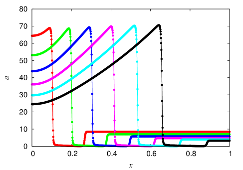
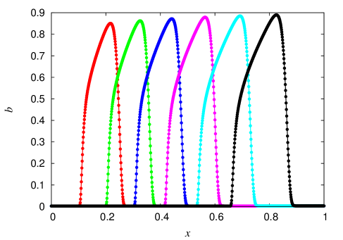
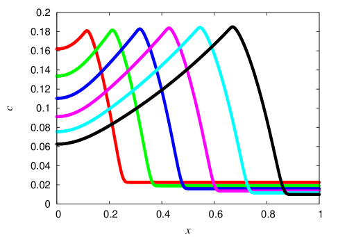
We consider problem (32) in a one–dimensional configuration with Neumann homogeneous boundary conditions, discretized on a uniform grid of 1024 cells over a space region of $[0,1]$. A standard, second order, centered finite volumes scheme is employed for the diffusion term. No grid adaptation is considered here in order to assess only the numerical errors related to the time integration schemes. To obtain an initial condition, we initialize the problem with a discontinuous profile close to the left boundary; we then integrate in time until the BZ wavefronts are fully developed. Figure 1 shows the time evolution of the propagating waves for a time window of $[0,1]$. In order to compute the local errors associated with the implicit solvers here considered, we define a reference solution for the resulting semi–discrete problem. The latter is chosen here as the solution obtained using the Radau5 scheme (51), computed with a fine tolerance: ${\eta_{\mathrm{RK}}}=10^{-14}$.

Figure 1: One–dimensional BZ propagating waves for variables $a$ (top left), $b$ (top right), and $c$ (bottom), at time intervals of $0.2$ within $[0,1]$ from left to right.

Figure 2: Local $L^{2}$–errors for stiff and non–stiff components, respectively, $a$ (top) and $c$ (bottom) using the SDIRK2, SDIRK3 and SDIRK4 schemes (left), and the Euler, Radau3 and Radau5 ones (right). Dashed lines of slopes 2 to 5 (top), 3 to 5 (bottom left), and 2, 4 and 5 (bottom right) are also depicted. Error estimates $err$ given by (27) are indicated with red bullets ($\color[rgb]{1,0,0}{\bullet}$) (top) for the SDIRK4 (left) and Radau5 (right) schemes.

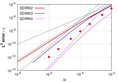
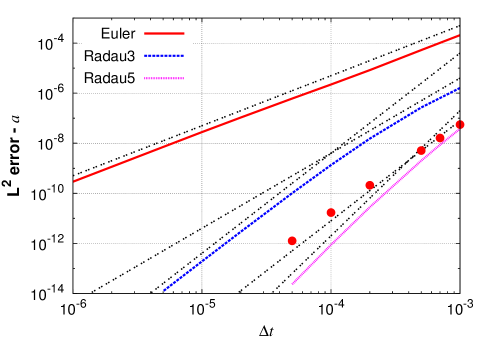
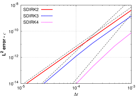
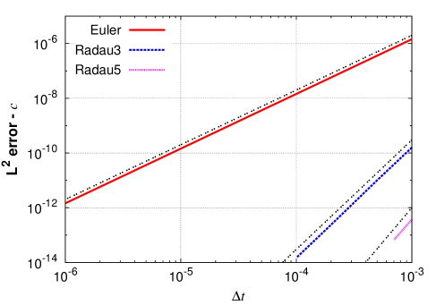
Starting from the solution at $t=0.5$, Figure 2 shows the local errors associated with each IRK scheme for different time steps. Both tolerances for the Newton and the linear solver are set to ${\eta_{\mathrm{Newt}}}={\eta_{\mathrm{LS}}}=10^{-14}$ in these computations. Notice that the stiffest variable, $a$, is directly subject to a time scale given by the small parameter $\mu=10^{-5}$. We are thus in practice interested in time steps larger than $10^{-5}$. Considering the stiff and non–stiff components of (32), $a$ and $c$, respectively, we see the following numerical behavior. For the stiff variable (see Figure 2 (top)), local errors of ${\mathcal{O}}(\Delta t^{p+1})$ tend to ${\mathcal{O}}(\Delta t^{q+1})$ for relatively large time steps. For the non–stiff variable (see Figure 2 (bottom)), the order reduction goes from ${\mathcal{O}}(\Delta t^{p+1})$ to ${\mathcal{O}}(\Delta t^{q+2})$. Local errors for variable $b$ (not shown), stiffer than $c$, also behave as the ones for the stiffest component, variable $a$. These results are consistent with the classical, theoretical bounds derived in [32] for stiff ODEs in singular perturbation form, that is, containing a small stiffness parameter given by $\mu$ in our case. These results highlight the importance of the stage order for IRK schemes and stiff problems. In this respect RadauIIA schemes perform better than SDIRK methods. The same can be said with respect to stiffly accurate schemes when comparing, for instance, SDIRK3 with Radau3; more accurate results are obtained with the latter. As a matter of fact, a well–known conclusion is that stiffly accurate schemes guarantee better accuracies for stiff problems [44, 1, 32]. Figure 2 also shows the error estimates $err$ given by (27) for both SDIRK4 and Radau5 schemes. Notice that the actual local errors are bounded by $err$, which in particular overestimates them since $err$ is computed using a third order, embedded scheme in both cases. Finally, it has to be remarked that higher order schemes perform better in terms of numerical accuracy than low order ones like the first order Euler method, even when order reduction appears and all methods show the same low order convergence.

4.1.2 Performance comparison

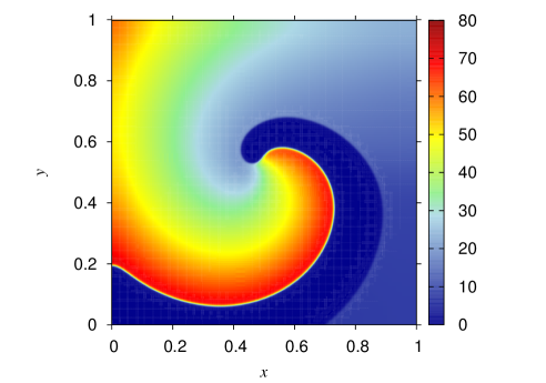
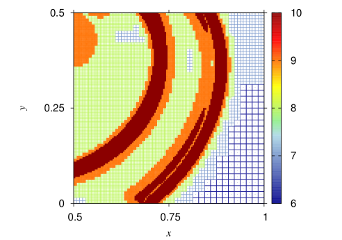
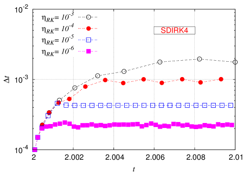
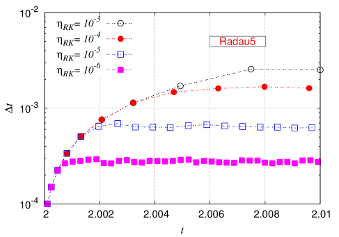
We now consider problem (32) in a two–dimensional configuration with Neumann homogeneous boundary conditions, using multiresolution analysis to adapt dynamically the spatial discretization grid. For the multiresolution analysis the following input parameters are considered: number of roots per direction, $N_{{\rm R}x}=N_{{\rm R}y}=1$; maximum grid–level, $J=10$; and accuracy tolerance, ${\eta_{\mathrm{MR}}}=10^{-3}$. The finest grid has a spatial resolution of $1024\times 1024$ over a computational domain of $[0,1]\times[0,1]$. We consider both SDIRK4 and Radau5 schemes with the following parameters: ${k_{\mathrm{Newt},\max}}=30$, ${k_{\mathrm{LS},{\mathbf{J}}}}={k_{\mathrm{Newt},\max}}$, and $\kappa=10^{-1}$, recalling that ${\eta_{\mathrm{LS}}}=\kappa{\eta_{\mathrm{Newt}}}=\kappa^{2}{\eta_{\mathrm{RK}}}$. The initial solution is taken at $t=2$, when the spiral waves are fully developed (see Figure 3), and the PDEs are then integrated until $t=2.01$. (See [24] for details on the initialization of this two–dimensional configuration.) The data compression, defined as the ratio in percentage between the active and the finest grids, is of about 15%.

Figure 3: Two–dimensional BZ propagating waves for variable $a$ at $t=2$ (left) and the corresponding adapted grid for the zoomed region $[0.5,1]\times[0,0.5]$ (right).

Figure 4: Time–stepping with different accuracy tolerances, ${\eta_{\mathrm{RK}}}$, for the SDIRK4 (left) and Radau5 (right) schemes.

Table 1: Time integration with SDIRK4 for $t\in[2,2.01]$: number of time steps, $n$; maximum time step used, $\max\Delta t_{n}$; maximum number of Newton iterations, $\max k$; maximum number of GMRES iterations, $\max{k_{\mathrm{LS}}}$; CPU time in seconds.

	${\eta_{\mathrm{RK}}}$	SDIRK4
		$n$	$\max\Delta t_{n}$	$\max k$ (per stage)	$\max{k_{\mathrm{LS}}}$	CPU time (s)
	$10^{-3}$	$11$	$1.95\times 10^{-3}$	$13$ ($3$)	$15$	$171.93$
	$10^{-4}$	$15$	$1.01\times 10^{-3}$	$17$ ($4$)	$13$	$269.28$
	$10^{-5}$	$26$	$4.65\times 10^{-4}$	$17$ ($4$)	$11$	$472.14$
	$10^{-6}$	$45$	$2.51\times 10^{-4}$	$19$ ($4$)	$10$	$837.62$

Table 2: Time integration with Radau5 for $t\in[2,2.01]$: number of time steps, $n$; maximum time step used, $\max\Delta t_{n}$; maximum number of Newton iterations, $\max k$; maximum number of GMRES iterations, $\max{k_{\mathrm{LS}}}$; CPU time in seconds.

	${\eta_{\mathrm{RK}}}$	Radau5
		$n$	$\max\Delta t_{n}$	$\max k$	$\max{k_{\mathrm{LS}}}$	CPU time (s)
	$10^{-3}$	$10$	$2.56\times 10^{-3}$	$5$	$60$	$892.98$
	$10^{-4}$	$12$	$1.64\times 10^{-3}$	$6$	$56$	$1268.11$
	$10^{-5}$	$19$	$6.97\times 10^{-4}$	$6$	$35$	$2311.30$
	$10^{-6}$	$37$	$2.98\times 10^{-4}$	$5$	$21$	$3416.22$

Figure 4 shows the evolution of time steps according to (30), considering $\alpha=1.5$ and $\Delta t_{0}=10^{-4}$ at $t=2$ for various accuracy tolerances: ${\eta_{\mathrm{RK}}}$ between $10^{-3}$ and $10^{-6}$. For this particular problem a roughly constant time step is attained, consistent with the quasi constant propagation speed of the wavefronts. Tables 1 and 2 gather information on the performance of both solvers during the time window $[2,2.01]$. As also seen in Figure 4, larger time steps for a given accuracy tolerance are used with the Radau5 scheme, even though both schemes consider a third order, embedded method to compute dynamically the integration time steps (28). For SDIRK4, increasing the accuracy of the Newton solver involves more iterations even when smaller time steps are considered, showing a rather low dependence on the time step size and a Newton solver piloted mainly by its accuracy tolerance. A different behavior is observed for Radau5 where smaller time steps involve roughly the same number of Newton iterations, regardless of the Newton accuracy tolerance, meaning that smaller time steps effectively improve the Newton solver. All this is a direct consequence of the initialization of the Newton solver; while for SDIRK4 the Newton solver at each stage is initialized using the previous stage solution and thus at some time within the current time step, this is not the case for the present Radau5 solver for which the larger the time step the worse the initial approximation. In terms of the iterative linear solver, the number of iterations decreases considerably with smaller time steps even when tighter convergence tolerances are considered. This is a direct consequence of the better preconditioning of the more diagonal–dominant matrices in (12) and (2.2.1) for relatively small time steps.

In terms of CPU time, following Tables 1 and 2 we can see that SDIRK4 is approximately $4$ to $5$ times faster than Radau5. Updating the grid together with the multiresolution operations takes approximately $10$ to $13\,$% for SDIRK4, whereas the time integration, $84$–$90\,$%. These numbers are within the range of values found in the literature for adaptive grid techniques (see, e.g., [20]). For Radau5 the multiresolution load goes down to $2\,$% with a roughly $98\,$% of the CPU time allocated to the time integration, showing a clear problem of performance. There are two main reasons why a straightforward implementation of Radau5 is not fully satisfactory. First of all, a better initialization of the Newton solver is required to improve the convergence rate of the linear solver, regardless of the solver considered. For example, in [34] (§ IV.8) all stages are initialized by extrapolating from the previous time step and using an interpolation polynomial based on the quadrature order conditions. Even if an adaptive grid technique can considerably reduce the increase of data storage that the latter procedure involves for multi–dimensional PDEs, we still have to introduce additional operations to initialize grid points that were not present during the previous time step. The second problem is related to the size of the algebraic systems which are basically tripled in the case of Radau5. The latter heavily impacts the performance of the linear solver. In this particular implementation, most of the overload is related to the preconditioning ILUT solver which was implemented as a black box, contrary to the GMRES solver. A tailored ILUT solver implemented specifically for this data structure may have already improved its performance before considering parallel computing implementations.

4.2 Ignition model of diffusion flames

We now consider the mathematical model derived in [50] to investigate the ignition dynamics of a diffusion flame, formed while a reactive layer is being rolled–up in a vortex. The hydrodynamics is decoupled from species and energy transport equations by adopting a standard thermo–diffusive approximation, leading to a reaction–diffusion–convection model. A two–dimensional computational domain is considered where pure and fresh hydrogen at temperature $T_{{\mathrm{F}},0}$ initially occupies the upper half part, while the remaining lower part of the domain is occupied by hot air at $T_{{\mathrm{O}},0}$. By defining a Schvab–Zeldo’vich variable $Z$ and a reduced temperature $\theta$ given by

$$\theta=\frac{T-T_{{\mathrm{O}},0}}{T_{{\mathrm{F}},0}-T_{{\mathrm{O}},0}},$$ (33)

the mathematical model is given by a system of equations of the form [50]:

$$\left.\begin{array}[]{l}\displaystyle\partial_{t}Z+v_{x}\partial_{x}Z+v_{y}\partial_{y}Z-\left(\partial^{2}_{x}Z+\partial^{2}_{y}Z\right)=0,\\[10.76385pt] \displaystyle\partial_{t}\theta+v_{x}\partial_{x}\theta+v_{y}\partial_{y}\theta-\left(\partial^{2}_{x}\theta+\partial^{2}_{y}\theta\right)=F(Z,\theta),\end{array}\right\}$$ (34)

$$F(Z,\theta)={\rm Da}\,\phi\chi Y_{{\mathrm{O}},0}\left[\frac{1-Z}{\phi\tau}+\frac{1}{\chi}(Z-\theta)\right]\left[Z+\frac{\tau}{\chi}(Z-\theta)\right]{\mathrm{e}}^{\left(-\tau_{a}/(1+\tau\theta)\right)},$$

with physical constant parameters: ${\rm Da}=1.65\times 10^{7}$, $\phi=34.782608696$, $\chi=50$, $Y_{{\mathrm{O}},0}=0.23$, $\tau=-0.7$, and $\tau_{a}=8$, corresponding to $T_{{\mathrm{F}},0}=300\,$K and $T_{{\mathrm{O}},0}=1000\,$K. The velocity field $(v_{x},v_{y})$ is given by a single vortex centered on the planar interface between the two media, which varies strongly in time and space. Its tangential velocity is given by

$$v_{\theta}(r,t)=\displaystyle\frac{{\rm Re}\,{\rm Sc}}{r}\left(1-{\mathrm{e}}^{-r^{2}/(4\,{\rm Sc}\,t)}\right),$$ (35)

where $r(x,y)$ stands for the distance to the vortex center $(x_{0},y_{0})=(0,0)$, and with Reynolds and Schmidt numbers of ${\rm Re}=1000$ and ${\rm Sc}=1$, respectively. In Cartesian coordinates, the velocity of a counter-clockwise rotating vortex is thus given by

$$v_{x}=\displaystyle\left(\frac{y-y_{0}}{r}\right)v_{\theta},\quad v_{y}=-\displaystyle\left(\frac{x-x_{0}}{r}\right)v_{\theta},\quad r=\left[(x-x_{0})^{2}+(y-y_{0})^{2}\right]^{1/2}.$$

The physics of the phenomenon can be briefly described as follows. A rotating vortex is introduced immediately at $t=0$. The resulting forced convection superposes to the diffusive mechanisms and accelerates the mixture of the gases. A diffusion flame then ignites along the contact surface of both media, taking into account the important difference of temperatures in those regions. Once the flame is completely ignited, it propagates outwards from the center of the computational domain. The complete phenomenon encompasses thus very different physical regimes like mixing, ignition, propagation, which can be characterized depending on the initial reactants configuration and on the imposed velocity field, as studied in detail in [50].

4.2.1 High order temporal approximations

We consider problem (34) in a two–dimensional configuration with Neumann homogeneous boundary conditions, using multiresolution analysis to adapt dynamically the spatial discretization grid. The convective term is discretized in space using a standard first–order upwind scheme. As before the multiresolution analysis is parametrized as follows: number of roots per direction, $N_{{\rm R}x}=N_{{\rm R}y}=1$; maximum grid–level, $J=10$; and accuracy tolerance, ${\eta_{\mathrm{MR}}}=10^{-3}$. The finest grid has thus a spatial resolution of $1024\times 1024$ over a computational domain of $[-1,1]\times[-1,1]$. The model is simulated for a time window of $[0,1.5\times 10^{-4}]$, using all the time integration solvers previously described. In all cases the following parameters were chosen: ${k_{\mathrm{Newt},\max}}=30$, ${k_{\mathrm{LS},{\mathbf{J}}}}={k_{\mathrm{Newt},\max}}$, and $\kappa=10^{-2}$. For this highly unsteady problem the number of active grid cells increases from approximately 3% of $1024^{2}$ for the initial inert configuration, up to 13% at the final time when the diffusion flame is fully ignited along the contact surface (see Figure 5). (See [23] for further details on the initialization of this problem.)

Figure 5: Two–dimensional ignition model. Temperature $T$ deduced from (33) at $t=1.5\times 10^{-4}$ (left) and the corresponding adapted grid for the zoomed region $[-1,0]\times[-1,0]$ (right).

Figure 6: Evolution of the maximum temperature $T_{max}$ using a time step of $\Delta t=10^{-5}$ for the SDIRK (top left) and Radau (top right) solvers. The solution computed with Radau5 and $\Delta t=10^{-6}$ is depicted with a solid black line. Similarly, time-adaptive solutions based on a tolerance of ${\eta_{\mathrm{RK}}}=10^{-3}$ are shown (bottom left). The various time steps considered for the SDIRK solvers are also illustrated (bottom right); in all cases, $\Delta t_{0}=10^{-8}$.

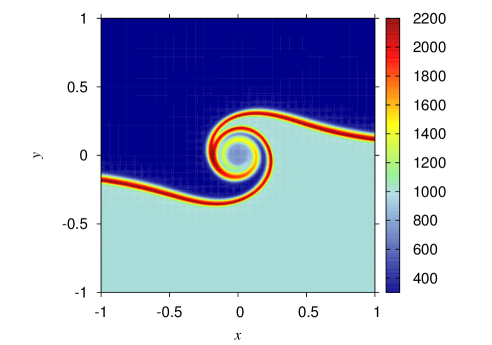
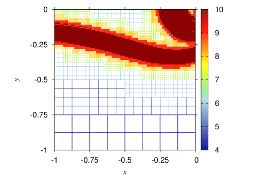
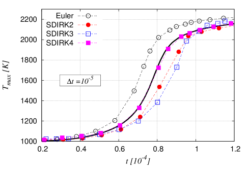
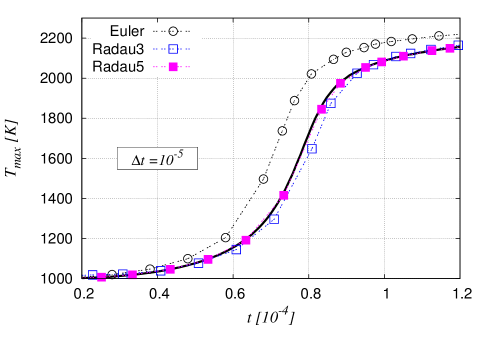
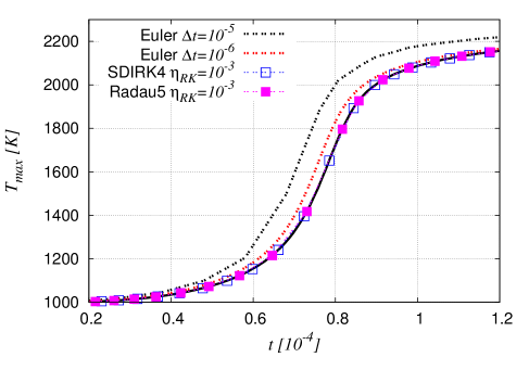
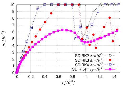
Figure 6 shows the time evolution of the maximum temperature $T_{max}$ throughout the computational domain. Notice that the initial $T_{max}$ corresponds to $T_{{\mathrm{O}},0}=1000\,$K, the hot air; however, the fuel is initially at a much lower temperature of $T_{{\mathrm{F}},0}=300\,$K and thus the local temperature changes are in fact even more dramatic. First, we consider a constant time step of $\Delta t=10^{-5}$, but with the time–stepping procedure given by (31). In all cases an initial time step of $\Delta t_{0}=10^{-8}$ was considered, taking into account that the velocity field (35) radically changes during the first time step. A tolerance of ${\eta_{\mathrm{LS}}}=10^{-5}$ is considered for the Newton solver. Figure 6 (top) clearly shows the difference between the approximations obtained with different discretization orders. As a reference solution we consider the one obtained with Radau5 and $\Delta t=10^{-6}$. The first order Euler solver introduces an ignition delay of the order of one time step. This delay is subsequently corrected by increasing the order of the time discretization with the same time step. Considering the third order approximations, SDIRK3 and Radau3, the latter performs much better for this particular problem because of its $L$–stability capabilities, given the strong transients that the stiff system (34) models. As a matter of fact, the $L$–stable SDIRK2 performs also better than SDIRK3. The difference of quality of the approximations can be further assessed by considering the final temperature at $t=1.5\times 10^{-4}$, once the ignition process is achieved and the strongest transients resolved. Final $T_{max}$ goes from $2254.09\,$K for the Euler solver to $2227.96\,$K and $2224.74\,$K for SDIRK4 and Radau5, respectively. For comparison, the reference Radau5 solution yields $2224.95\,$K. With a smaller time step of $\Delta t=10^{-6}$, the Euler solution still shows a considerable difference (see Figure 6 (bottom left)) with a final $T_{max}$ of $2219.54\,$K. All the other solvers with $\Delta t=10^{-6}$ yield solutions with less than $0.3\,$K of difference with respect to the Radau5 solution, except for SDIRK3 with about $1\,$K of difference.

As an illustration, Figure 6 (bottom right) also depicts the time steps considered for the various SDIRK solvers. Recalling that the time–stepping strategy is actually influenced by the performance of the Newton and linear solvers, we can see the impact of strong physical changes during the ignition process as all solvers need to use at some point smaller time steps. Similar behaviors are observed for the Euler and Radau solvers (not shown). In particular it can be seen again how the non $L$–stable SDIRK3 is the most affected solver. Notice that for these numerical experiments we have chosen a relatively large ${k_{\mathrm{Newt},\max}}$ as this allows for larger time steps according to (29); consequently, ${k_{\mathrm{LS},{\mathbf{J}}}}$ is also large and the Jacobians are never recomputed. Time steps are thus reduced due to a bad convergence rate of the Newton solver; a more conservative lower ${k_{\mathrm{Newt},\max}}$ prevents this bad convergence rates since time steps would not even attain $10^{-5}$. In general a careful tuning of parameters should be conducted with this “constant” time step strategy in order to get the best possible performance. This tuning can be highly problem–dependent. That is why a time–stepping strategy based on an accuracy tolerance is very convenient, as the time steps can be effectively adapted to the various physical scenarios within a prescribed accuracy, while reducing the importance of the many parameters related to the Newton and linear solvers. Time–adaptive solutions are shown in Figure 6 (bottom left) for SDIRK4 and Radau5 with ${\eta_{\mathrm{RK}}}=10^{-3}$. In terms of CPU time, with $\Delta t=10^{-5}$ the Euler solver takes approximately $3.6$ minutes, compared to $5$ and $14.9$ for SDIRK4 and Radau5, respectively; but the physics simulated with the first order method diverges considerably from the right one. The time–adaptive SDIRK4 with ${\eta_{\mathrm{RK}}}=10^{-3}$ takes approximately $4$ minutes, becoming a very promising alternative to the cheaper but less accurate Euler scheme, especially if one takes into account that a more accurate Euler solver with $\Delta t=10^{-6}$ takes about $6$ minutes.

5 Concluding remarks

We have considered high order, implicit integration schemes to solve stiff multi–dimensional PDEs on adaptive multiresolution grids. Such an adaptive technique yields highly compressed representations within a user–prescribed accuracy tolerance, considerably reducing the computational requirements of implicit Runge–Kutta schemes. In particular a competitive time–space adaptive strategy was introduced to simulate models involving different physical scenarios with a broad spectrum of time and space scales within a user–specified level of accuracy. By designing an appropriate procedure to evaluate functions and represent linear systems within the multiresolution data structure, we have implemented several implicit Runge–Kutta schemes of SDIRK– and RadauIIA–type. The resulting linear systems are completely independent of the grid generation or any other grid–related data structure or geometric consideration. Solving the algebraic problems constitute then a separate aspect from the multiresolution analysis itself, while the same procedure remains perfectly valid for other space adaptive techniques.

Three stiff models have been investigated to assess the computational performance of the numerical strategy in terms of accuracy and CPU time. The computational analyses have thus proved that stiff PDEs can be effectively approximated with high order time discretization schemes with very limited computational resources. In particular SDIRK schemes require roughly the same amount of memory than a standard, low order Euler method. More memory–demanding RadauIIA schemes can also be employed in conjunction with adapted grids; however, as previously discussed, further enhancements are required to achieve better computational performances. It was also shown that even in the presence of order reduction, high order schemes yield more accurate solutions than low order ones. The advantages of high order discretizations have been especially highlighted when dealing with highly unsteady problems. However, for problems of even larger size parallel computing capabilities must be developed within the current context to achieve overall satisfactory results. Additionally, high order space discretization schemes, well–suited for implicit schemes [43, 42, 18], could be also considered in conjunction with grid adaptation to further enhance the computational performance. These issues constitute particular topics of our current research.

Appendix A Details on multiresolution analysis

Defining $\Omega_{\lambda}:=\Omega_{j,k}$, we denote $|\lambda|:=j$ if $\lambda\in S_{j}$, while subscript $k\in\Delta_{j}\subset{\mathbb{Z}}^{d}$ corresponds to the position of the cell within $S_{j}$. For instance, in Cartesian coordinates the univariate dyadic intervals in ${\mathbb{R}}$ are given by

$$\Omega_{\lambda}=\Omega_{j,k}:=]2^{-j}k,2^{-j}(k+1)[,\ \lambda\in S_{j}:=\{(j,k)\ \mathrm{s.t.}\ j\in(0,1,\ldots,J),\,k\in{\mathbb{Z}}\},$$ (36)

and the same follows for higher dimensions.

Following [17], the projection operator $P^{j}_{j-1}$ maps ${\mathbf{U}}_{j}$ to ${\mathbf{U}}_{j-1}$. It is obtained through exact averages computed at the finer level by

$$u_{\lambda}=|\Omega_{\lambda}|^{-1}\sum_{|\mu|=|\lambda|+1,\Omega_{\mu}\subset\Omega_{\lambda}}|\Omega_{\mu}|u_{\mu}.$$ (37)

As far as grids are nested, this projection operator is exact and unique [16]. On the other hand, the prediction operator $P^{j-1}_{j}$ maps ${\mathbf{U}}_{j-1}$ to an approximation $\widehat{{\mathbf{U}}}_{j}$ of ${\mathbf{U}}_{j}$. There are several choices to define $P^{j-1}_{j}$, but two basic constraints are usually imposed:

1. The prediction is local, i.e., $\widehat{u}_{\lambda}$ depends on the values $u_{\mu}$ on a finite stencil $R_{\lambda}$ surrounding $\Omega_{\lambda}$, where $|\lambda|=|\mu|+1$.

2. The prediction is consistent with the projection in the sense that

   $$u_{\lambda}=|\Omega_{\lambda}|^{-1}\sum_{|\mu|=|\lambda|+1,\Omega_{\mu}\subset\Omega_{\lambda}}|\Omega_{\mu}|\widehat{u}_{\mu};$$ (38)

   i.e., one can retrieve the coarse cell averages from the predicted values:

   $$P_{j-1}^{j}\circ P_{j}^{j-1}={\mathrm{Id}}.$$ (39)

With these operators, for each cell $\Omega_{\lambda}$ the prediction error or detail is defined as the difference between the exact and predicted values,

$$d_{\lambda}:=u_{\lambda}-\widehat{u}_{\lambda},$$ (40)

or in terms of inter–level operations: $d_{\lambda}=u_{\lambda}-P_{|\lambda|}^{|\lambda|-1}\circ P_{|\lambda|-1}^{|\lambda|}u_{\lambda}$. The consistency property (38) and the definitions of the projection operator (37) and of the detail (40) imply

$$\sum_{|\lambda|=|\mu|+1,\Omega_{\lambda}\subset\Omega_{\mu}}|\Omega_{\lambda}|d_{\lambda}=0.$$ (41)

We can then construct as shown in [17] a detail vector defined as ${\mathbf{D}}_{j}:=(d_{\lambda})_{\lambda\in\nabla_{j}}$, where the set $\nabla_{j}\subset S_{j}$ is obtained by removing for each $\mu\in S_{j-1}$ one $\lambda\in S_{j}$ ($\Omega_{\lambda}\subset\Omega_{\mu}$) in order to avoid redundancy (considering (41)) and to get the one–to–one correspondence (4).

Given a set of indices $\Lambda\subset\nabla^{J}$, where $\nabla^{J}:=\bigcup_{j=0}^{J}\nabla_{j}$ with $\nabla_{0}:=S_{0}$, the thresholding operator ${\mathcal{T}}_{\Lambda}$ is such that leaves unchanged the components $d_{\lambda}$ of the multi–scale representation ${\mathbf{M}}_{J}$ in (5) if $\lambda\in\Lambda$, and replaces it by $0$ otherwise. Defining the level–dependent threshold values $(\epsilon_{0},\epsilon_{1},\ldots,\epsilon_{J})$, the set $\Lambda$ is given by

$$\lambda\in\Lambda\ {\rm if}\ \|d_{\lambda}\|_{L^{p}}\geq\epsilon_{|\lambda|}.$$ (42)

Applying ${\mathcal{T}}_{\Lambda}$ on the multi–scale decomposition ${\mathbf{M}}_{J}$ of ${\mathbf{U}}_{J}$ amounts then to building the multiresolution approximation ${\mathbf{U}}_{J}^{\epsilon}:={\mathcal{A}}_{\Lambda}{\mathbf{U}}_{J}$ to ${\mathbf{U}}_{J}$, where the operator ${\mathcal{A}}_{\Lambda}$ is given by

$${\mathcal{A}}_{\Lambda}:={\mathcal{M}}^{-1}{\mathcal{T}}_{\Lambda}{\mathcal{M}},$$

in which all details below a certain level of regularity have been discarded. The bound (6) is thus verified with the level–dependent threshold values:

$$\epsilon_{j}=2^{d(j-J)/2}{\eta_{\mathrm{MR}}},\quad j=0,1,\ldots,J.$$

Appendix B Details on implicit Runge–Kutta schemes

The solution ${\mathbf{U}}(t_{0}+\Delta t)$ of problem (7) is approximated by ${\mathbf{U}}_{1}$, computed as

$${\mathbf{g}}_{i}={\mathbf{U}}_{0}+\Delta t\displaystyle\sum_{j=1}^{s}a_{ij}{\mathbf{F}}\left(t_{0}+c_{j}\Delta t,{\mathbf{g}}_{j}\right),\qquad i=1,\ldots,s;$$ (43)

$${\mathbf{U}}_{1}={\mathbf{U}}_{0}+\Delta t\displaystyle\sum_{j=1}^{s}b_{j}{\mathbf{F}}\left(t_{0}+c_{j}\Delta t,{\mathbf{g}}_{j}\right),$$ (44)

where the time dependence for ${\mathbf{F}}({\mathbf{U}}(t))$ was added for the sake of clarity. Following the approach established in [34], the set of arrays ${\mathbf{z}}_{1},\ldots,{\mathbf{z}}_{s}$, are defined such that ${\mathbf{z}}_{i}={\mathbf{g}}_{i}-{\mathbf{U}}_{0}$, $i=1,\ldots,s$, and hence,

$${\mathbf{z}}_{i}=\Delta t\displaystyle\sum_{j=1}^{s}a_{ij}{\mathbf{F}}(t_{0}+c_{j}\Delta t,{\mathbf{U}}_{0}+{\mathbf{z}}_{j}),\qquad i=1,\ldots,s.$$ (45)

Therefore, knowing the solution ${\mathbf{z}}_{1},\ldots,{\mathbf{z}}_{s}$ implies an explicit formula for ${\mathbf{U}}_{1}$ in (44), for which $s$ additional function evaluations are required. These extra computation can nevertheless be avoided if the matrix ${\boldsymbol{A}}$ is nonsingular, as seen in (9).

A standard iterative Newton solver for system (8) amounts to solving at each iteration a linear system that requires the inversion of the block–matrix:

$$\left(\begin{array}[]{ccc}{\mathbf{Id}}_{m\times N}-\Delta ta_{11}{\mathbf{J}}_{1}({\mathbf{z}}_{1})&\ldots&-\Delta ta_{1s}{\mathbf{J}}_{s}({\mathbf{z}}_{s})\\ \vdots&\ddots&\vdots\\ -\Delta ta_{s1}{\mathbf{J}}_{1}({\mathbf{z}}_{1})&\ldots&{\mathbf{Id}}_{m\times N}-\Delta ta_{ss}{\mathbf{J}}_{s}({\mathbf{z}}_{s})\end{array}\right),$$ (46)

where ${\mathbf{J}}_{i}({\mathbf{z}}_{i}):=\partial_{{\mathbf{U}}}{\mathbf{F}}(t_{0}+c_{i}\Delta t,{\mathbf{U}}_{0}+{\mathbf{z}}_{i})$, $i=1,\ldots,s$, stands for the Jacobian $\partial_{{\mathbf{U}}}{\mathbf{F}}:=\partial{\mathbf{F}}({\mathbf{U}})/\partial{\mathbf{U}}$ of size $m\times N$, evaluated at the various inner stages. Following [34], the simplified Newton solver (12) approximates all Jacobians in (46) as

$${\mathbf{J}}_{i}({\mathbf{z}}_{i})\approx{\mathbf{J}}_{0}:=\partial_{{\mathbf{U}}}{\mathbf{F}}(t_{0},{\mathbf{U}}_{0}),\quad i=1,\ldots,s.$$ (47)

Appendix C Butcher tableau of IRK schemes

We consider a two–stage SDIRK scheme [33] (Table II.7.2) given by

$$\begin{tabular}[]{c|c c }$\gamma$&$\gamma$&\\ $1-\gamma$&$1-2\gamma$&$\gamma$\\ \hline\cr&$1/2$&$1/2$\end{tabular}\qquad d_{1}=\frac{3\gamma-1}{2\gamma^{2}},\quad d_{2}=\frac{1}{2\gamma}.$$ (48)

With $\gamma=(2\pm\sqrt{2})/2$ the method (48) is of second order ($p=2$, $s=p$) and $L$–stable. For $\gamma=(3+\sqrt{3})/6$ it becomes a third order scheme ($p=3$, $s=p-1$), but is only $A$–stable. The fourth order SDIRK4 scheme proposed in [34] (Table IV.6.5) with $s=5$, is

$$\frac{1}{4}$$

(49)

The latter is an $L$–stable and stiffly accurate method.

The RadauIIA methods of order 3 and 5 are given, respectively, by ([34] Tables IV.5.5 and IV.5.6)

$$\frac{1}{3}$$

(50)

and

$$\frac{4-\sqrt{6}}{10}$$

(51)

Appendix D Numerical computation of Jacobians

The Jacobian at a given stage $s$: ${\mathbf{J}}_{s}=\partial_{{\mathbf{U}}}{\mathbf{F}}({\mathbf{U}}_{s})=(J^{s}_{i,j})_{i,j\in{\rm I}^{n}_{\mathrm{L}}}$, needs to be numerically approximated at each leaf of the adapted grid. The latter is done by considering for each $i=1,2,\ldots,N^{n}_{\mathrm{L}}$, $\lambda=h_{n}^{-1}(i)$, the following expression

$$J^{s}_{h_{n}(\lambda),h_{n}(\mu)}=\frac{F_{\lambda}({\mathbf{U}}_{s}+\delta_{\mu}{\mathbf{1}}_{\mu})-F_{\lambda}({\mathbf{U}}_{s})}{\delta_{\mu}},\qquad\forall\mu\in R_{\varPhi}[\lambda],$$ (52)

with the one–dimensional array ${\mathbf{1}}_{\mu}\in R^{N^{n}_{\mathrm{L}}}$, such that $\mathbf{1}_{\mu}(i)=1$ for $i=h_{n}(\mu)$ and $\mathbf{1}_{\mu}(i)=0$, otherwise; $\delta_{\mu}$ is a small perturbation taken here as $\delta_{\mu}=(10^{-16}\times\max(10^{-5},|u^{s}_{\mu}|))^{0.5}$, following [34]. Recalling (20) and the conservation property, the latter perturbation is limited in practice to the stencil $R_{\varPhi}^{+}[\lambda]$. That is, perturbed fluxes $\varPhi^{+}_{\lambda}({\mathbf{U}}_{s}+\delta_{\mu}{\mathbf{1}}_{\mu})$ are evaluated for all $\mu\in R_{\varPhi}^{+}[\lambda]$ to compute $J^{s}_{h_{n}(\lambda),h_{n}(\mu)}$, while $-\varPhi^{+}_{\lambda}({\mathbf{U}}_{s}+\delta_{\mu}{\mathbf{1}}_{\mu})$ is used to compute the Jacobian entry at cell $\mu$ due to perturbed cell $\lambda$: $J^{s}_{h_{n}(\mu),h_{n}(\lambda)}$. Notice that only cells contained in the adapted grid, i.e., the leaves, are perturbed to compute the Jacobians. Close to level interfaces where a ghost–cell $\Omega_{\nu}$ might be contained in the flux stencil, we perturb the latter with the same $\delta_{\mu}$ corresponding to its parent $\Omega_{\mu}\supset\Omega_{\nu}$, which is of course a leaf. Geometric proportions must then be taken into account when transferring fluxes between cells of different resolution.

Appendix E Embedded Runge–Kutta schemes

The error measures used in this work rely upon the lower order embedded IRK schemes introduced in [34] for the SDIRK4 and Radau5 schemes. For SDIRK4, the error approximation $err$ is computed from

$$\hat{{\mathbf{U}}}_{1}-{\mathbf{U}}_{1}=\sum_{i=1}^{5}e_{i}{\mathbf{z}}_{i},$$ (53)

with coefficients ${\boldsymbol{e}}^{T}:=(e_{1},\ldots,e_{5})=(23/6,17/12,-125/4,85/3,1)$, which is accurate to third order ($\hat{p}=3$). In the case of Radau5, we consider

$$\hat{{\mathbf{U}}}_{1}-{\mathbf{U}}_{1}=K\Delta t{\mathbf{F}}(t_{0},{\mathbf{U}}_{0})+\sum_{i=1}^{3}e_{i}{\mathbf{z}}_{i},$$ (54)

with $K=10^{-1}$, ${\boldsymbol{e}}^{T}=K(-13-7\sqrt{6},-13+7\sqrt{6},-1)$, which is also accurate to third order ($\hat{p}=3$). As pointed out in [40] neither of these error estimates has $A$–stability properties. A remedy was proposed in [34] for their Radau5 solver, that is currently not implemented in our code.

References

- [1] R. Alexander. Diagonally implicit Runge-Kutta methods for stiff O.D.E.’s. SIAM J. Numer. Anal., 14(6):1006–1021, 1977.
- [2] O. Axelsson. A note on a class of strongly A-stable methods. BIT Numer. Math., 12:1–4, 1972.
- [3] M. Bendahmane, R. Bürger, R. Ruiz-Baier, and K. Schneider. Adaptive multiresolution schemes with local time stepping for two-dimensional degenerate reaction-diffusion systems. Appl. Numer. Math., 59(7):1668–1692, 2009.
- [4] B.A.V. Bennett, C.S. McEnally, L.D. Pfefferle, M.D. Smooke, and M.B. Colket. Computational and experimental study of the effects of adding dimethyl ether and ethanol to nonpremixed ethylene/air flames. Combust. Flame, 156(6):1289–1302, 2009.
- [5] B.A.V. Bennett and M.D. Smooke. Local rectangular refinement with application to axisymmetric laminar flames. Combust. Theor. Model., 2(3):221–258, 1998.
- [6] B.A.V. Bennett and M.D. Smooke. Local rectangular refinement with application to nonreacting and reacting fluid flow problems. J. Comput. Phys., 151(2):684–727, 1999.
- [7] B.L. Bihari and A. Harten. Multiresolution schemes for the numerical solution of 2-D conservation laws I. SIAM J. Sci. Comput., 18(2):315–354, 1997.
- [8] H. Bijl and M.H. Carpenter. Iterative solution techniques for unsteady flow computations using higher order time integration schemes. Int. J. Numer. Meth. Fluids, 47:857–862, 2005.
- [9] H. Bijl, M.H. Carpenter, V.N. Vatsa, and C.A. Kennedy. Implicit time integration schemes for the unsteady compressible Navier–Stokes equations: Laminar flow. J. Comput. Phys., 179(1):313–329, 2002.
- [10] K. Brix, S. Melian, S. Müller, and M. Bachmann. Adaptive multiresolution methods: Practical issues on data structures, implementation and parallelization. ESAIM: Proc., 34:151–183, 2011.
- [11] R. Bürger, R. Ruiz-Baier, K. Schneider, and M. Sepúlveda. Fully adaptive multiresolution schemes for strongly degenerate parabolic equations in one space dimension. ESAIM: Math. Model. Numer. Anal., 42:535–563, 2008.
- [12] J.C. Butcher. Implicit Runge-Kutta processes. Math. Comp., 18:50–64, 1964.
- [13] J.C. Butcher. Integration processes based on Radau quadrature formulas. Math. Comp., 18:233–244, 1964.
- [14] M.H. Carpenter, C.A. Kennedy, H. Bijl, S.A. Viken, and V.N. Vatsa. Fourth–order Runge–Kutta schemes for fluid mechanics applications. J. Sci. Comput., 25:157–194, 2005.
- [15] F.H. Chipman. A-stable Runge-Kutta processes. BIT Numer. Math., 11:384–388, 1971.
- [16] A. Cohen. Wavelet Methods in Numerical Analysis, volume 7. Elsevier, Amsterdam, 2000.
- [17] A. Cohen, S.M. Kaber, S. Müller, and M. Postel. Fully adaptive multiresolution finite volume schemes for conservation laws. Math. Comp., 72:183–225, 2003.
- [18] R. Dobbins and M.D. Smooke. A fully implicit, compact finite difference method for the numerical solution of unsteady laminar flames. Flow Turbul. Combust., 85(3-4):763–799, 2010.
- [19] M. Domingues, S. Gomes, O. Roussel, and K. Schneider. Adaptive multiresolution methods. ESAIM: Proc., 34:1–96, 2011.
- [20] M. Duarte. Méthodes numériques adaptatives pour la simulation de la dynamique de fronts de réaction multi-échelles en temps et en espace. PhD thesis, Ecole Centrale Paris, France, 2011.
- [21] M. Duarte, Z. Bonaventura, M. Massot, and A. Bourdon. A numerical strategy to discretize and solve the Poisson equation on dynamically adapted multiresolution grids for time-dependent streamer discharge simulations. J. Comput. Phys., 289:129–148, 2015.
- [22] M. Duarte, Z. Bonaventura, M. Massot, A. Bourdon, S. Descombes, and T. Dumont. A new numerical strategy with space-time adaptivity and error control for multi-scale streamer discharge simulations. J. Comput. Phys., 231:1002–1019, 2012.
- [23] M. Duarte, S. Descombes, C. Tenaud, S. Candel, and M. Massot. Time-space adaptive numerical methods for the simulation of combustion fronts. Combust. Flame, (160):1083–1101, 2013.
- [24] M. Duarte, M. Massot, S. Descombes, C. Tenaud, T. Dumont, V. Louvet, and F. Laurent. New resolution strategy for multi-scale reaction waves using time operator splitting, space adaptive multiresolution and dedicated high order implicit/explicit time integrators. SIAM J. Sci. Comput., 34(1):A76–A104, 2012.
- [25] T. Dumont, M. Duarte, S. Descombes, M.-A. Dronne, M. Massot, and V. Louvet. Simulation of human ischemic stroke in realistic 3D geometry. Commun. Nonlinear Sci. Numer. Simul., 18(6):1539–1557, 2013.
- [26] B.L. Ehle. High order A-stable methods for the numerical solution of systems of DEs. BIT Numer. Math., 8:276–278, 1968.
- [27] B.L. Ehle. On Padé approximations to the exponential function and A-stable methods for the numerical solution of initial value problems. Research Report CSRR 2010, 1969.
- [28] I.R. Epstein and J.A. Pojman. An Introduction to Nonlinear Chemical Dynamics. Oxford University Press, 1998. Oscillations, Waves, Patterns and Chaos.
- [29] R.J. Field, E. Koros, and R.M. Noyes. Oscillations in chemical systems. II. Thorough analysis of temporal oscillation in the bromate–cerium–malonic acid system. J. Amer. Chem. Soc., 94(25):8649–8664, 1972.
- [30] P. Gray and S.K. Scott. Chemical Oscillations and Instabilites. Oxford Univ. Press, 1994.
- [31] A. Guillon and F.L. Soulé. La résolution numérique des problèmes différentiels aux conditions initiales par des méthodes de collocation. RAIRO Anal. Numér. Ser. Rouge, v. R-3, pages 17–44, 1969.
- [32] E. Hairer, C. Lubich, and M. Roche. Error of Runge-Kutta methods for stiff problems studied via differential algebraic equations. BIT Numer. Math., 28:678–700, 1988.
- [33] E. Hairer, S. P. Nørsett, and G. Wanner. Solving Ordinary Differential Equations I. Springer-Verlag, Berlin, 1987. Nonstiff Problems.
- [34] E. Hairer and G. Wanner. Solving Ordinary Differential Equations II. Springer-Verlag, Berlin, 2nd edition, 1996. Stiff and Differential-Algebraic Problems.
- [35] A. Harten. Adaptive multiresolution schemes for shock computations. J. Comput. Phys., 115:319–338, 1994.
- [36] A. Harten. Multiresolution algorithms for the numerical solution of hyperbolic conservation laws. Comm. Pure and Applied Math., 48:1305–1342, 1995.
- [37] N. Hovhannisyan and S. Müller. On the stability of fully adaptive multiscale schemes for conservation laws using approximate flux and source reconstruction strategies. IMA J. Numer. Anal., 30(4):1256–1295, 2010.
- [38] S. Isono and D. Zingg. A Runge-Kutta-Newton-Krylov algorithm for fourth-order implicit time marching applied to unsteady flows. AIAA Paper 2004-0433, 2004.
- [39] D.A. Knoll and D.E. Keyes. Jacobian-free Newton-Krylov methods: A survey of approaches and applications. J. Comput. Phys., 193(2):357–397, 2004.
- [40] A. Kværnø. Singly diagonally implicit Runge-Kutta methods with an explicit first stage. BIT Numer. Math., 44(3):489–502, 2004.
- [41] S. Müller. Adaptive Multiscale Schemes for Conservation Laws, volume 27. Springer-Verlag, 2003.
- [42] M. Noskov, M. Benzi, and M.D. Smooke. An implicit compact scheme solver for two-dimensional multicomponent flows. Comput. Fluids, 36(2):376–397, 2007.
- [43] M. Noskov and M.D. Smooke. An implicit compact scheme solver with application to chemically reacting flows. J. Comput. Phys., 203(2):700–730, 2005.
- [44] A. Prothero and A. Robinson. On the stability and accuracy of one-step methods for solving stiff systems of ordinary differential equations. Math. Comp., 28(125):145–162, 1974.
- [45] R. Radau. Étude sur les formules d’approximation qui servent à calculer la valeur numérique d’une intégrale definie. J. Math. Pures Appl., 6:283–336, 1880.
- [46] O. Roussel, K. Schneider, A. Tsigulin, and H. Bockhorn. A conservative fully adaptive multiresolution algorithm for parabolic PDEs. J. Comput. Phys., 188(2):493–523, 2003.
- [47] Y. Saad. ILUT: A dual threshold incomplete LU factorization. Numer. Linear Algebra Appl., 1(4):387–402, 1994.
- [48] Y. Saad and M. Schultz. GMRES: A generalized minimal residual algorithm for solving nonsymmetric linear systems. SIAM J. Sci. Stat. Comp., 7(3):856–869, 1986.
- [49] M.D. Smooke. The computation of laminar flames. Proc. Combust. Inst., 34(1):65–98, 2013.
- [50] D. Thévenin and S. Candel. Ignition dynamics of a diffusion flame rolled up in a vortex. Phys. Fluids, 7(2):434–445, 1995.
- [51] L. Tosatto, B.A.V. Bennett, and M.D. Smooke. Parallelization strategies for an implicit Newton-based reactive flow solver. Combust. Theor. Model., 15(4):455–486, 2011.
- [52] K. Wright. Some relationships between implicit Runge-Kutta, collocation and Lanczos methods, and their stability properties. BIT Numer. Math., 10:217–227, 1971.