Initial State Quantum Fluctuations in the Little Bang

Abstract

We review recent developments in the ab-initio theoretical description of the initial state in heavy-ion collisions. We emphasize the importance of fluctuations, both for the phenomenological description of experimental data from the Relativistic Heavy Ion Collider (RHIC) and the Large Hadron Collider (LHC), and the theoretical understanding of the non-equilibrium early time dynamics and thermalization of the medium.

I Introduction

Heavy Ion Collisions, devoted to probe the hot and dense phases of nuclear matter, may in principle be described by Quantum Chromodynamics (QCD) – the microscopic theory of quarks and gluons. However, due to the extremely complicated dynamics at play in the collisions, such an ab initio description appears hopeless. Instead, one resorts to various mesoscopic descriptions, that integrate out many of the microscopic details.

A crucial challenge in such a coarse graining procedure is to identify the relevant aspects of the underlying fundamental description that must be kept in order to correctly describe the system. In the underlying quantum field theory, renormalizability implies that quantum fluctuations are important down to spatial scales of the order of the typical inverse momentum, while smaller fluctuations are simply encapsulated in the scale dependence of a few parameters such as the coupling constant. But in the more macroscopic descriptions used in heavy ion collisions there is no such clear procedure.

The purpose of this review is to discuss the various sources of fluctuations, and their role in the observable outcome of the collisions.

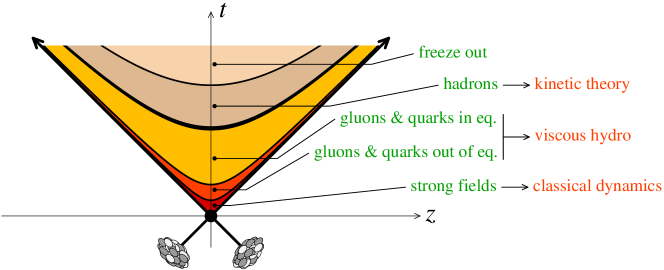
Figure 1: Successive stages of a heavy ion collision.

I.1 Hydrodynamics in heavy ion collisions

Over many years, relativistic fluid dynamics has proven to be the most successful effective theory to describe the bulk dynamics of heavy ion collisions. Early on, ideal hydrodynamics was able to describe many qualitative features of the experimental data, including a large elliptic flow $v_{2}$ and mass splitting between the $v_{2}$ coefficients for different particle species. This gave the first indication that the matter created in heavy ion collisions at the Relativistic Heavy Ion Collider (RHIC) is close to a perfect fluid Hirano and Tsuda (2002); Kolb and Heinz (2003); Huovinen (2003). This was confirmed later at the Large Hadron Collider (LHC).

With the development of viscous relativistic hydrodynamic simulations and comparison to experimental data from heavy ion collisions Romatschke and Romatschke (2007) the value of the shear viscosity to entropy density ratio $\eta/s$ could be determined to be close to the conjectured strong coupling limit of $\eta/s=1/4\pi$ obtained from the AdS/CFT correspondence Policastro et al. (2001); Kovtun et al. (2005). Since then much progress has been made. In particular the inclusion of event-by-event fluctuations in the initial state of viscous hydrodynamics Schenke et al. (2011); Bozek and Broniowski (2012); Karpenko et al. (2015) has turned out to be of great importance. For recent reviews on the status of relativistic fluid dynamics for heavy ion collisions see Heinz and Snellings (2013); Gale et al. (2013a); de Souza et al. (2015); Jeon and Heinz (2015).

I.2 Relevance of initial state fluctuations for data interpretation

The role of fluctuations in the transverse geometry of the collision system was realized when experimentally studying the elliptic flow in central Cu+Cu collisions at RHIC Alver et al. (2007). The large observed $v_{2}$ could only be explained when the shape of the overlap region was calculated relative to an axis determined by the fluctuating participants. This concept turned out to have far reaching consequences. In particular it allowed for the explanation of the structure of two particle correlations in their pseudo-rapidity $\eta_{p}$ and azimuthal angular difference, namely the so called ridge. Its structure around $\Delta\phi=\pi$ in central collisions is due to the contribution of the odd harmonic $v_{3}$, which in the absence of fluctuations would be zero Mishra et al. (2008); Alver and Roland (2010); Alver et al. (2010).

The combined analysis of all $v_{n}$ and their event-by-event distributions Aad et al. (2013) has allowed to constrain the initial state and its fluctuations as well as the shear viscosity of the medium. The event-by-event distributions when scaled by the mean $v_{n}$ are largely independent of the detailed transport parameters of the medium Niemi et al. (2013), which makes them ideal observables to constrain features of the initial state. In fact, currently there are only a few initial state models that describe all $v_{n}$ distributions $(n=2,3,4)$ for all experimentally measured centralities. Most prominently, those are the IP-Glasma model Schenke et al. (2012a, b); Gale et al. (2013b), that we will discuss in more detail below, and the EKRT framework Niemi et al. (2015). Both models include saturation effects and lead to similar energy deposition in the transverse plane. In Moreland et al. (2015) it was shown that the relevant feature to describe the experimental data is that the initial entropy density is proportional to the product of thickness functions.

In Section II.4 we will describe in more detail the relevance of the initial energy deposition and fluctuations for describing experimental data using the IP-Glasma model coupled to fluid dynamic calculations.

I.3 Fast thermalization: Is it necessary?

Hydrodynamics is an expansion around the energy momentum tensor of an ideal fluid at rest. Since the baseline of this expansion is a fluid in local thermal equilibrium, it is often assumed that near-equilibrium is a prerequisite for hydrodynamics.

Data on flow observables indicate a very effective transfer from spatial anisotropy to momentum anisotropy. However, this transfer would be impaired by the strong dissipative effects that occur during the rearrangement of the internal degrees of freedom of an off-equilibrium system. Moreover, for a successful description of bulk observables in heavy ion collisions, the hydrodynamical evolution should start very shortly after the collision, at times $\tau\lesssim 1$ fm/c.

However, there is no direct evidence from data that the system is indeed close to equilibrium. Although the above argument suggests that a certain amount of pre-equilibration must have taken place before hydrodynamics becomes a valid description, there are examples (exactly solvable AdS/CFT models Heller et al. (2012), or systems also studied in kinetic theory Kurkela and Zhu (2015)) where the deviation of the energy-momentum tensor from its ideal form is of order one, and hydrodynamics nevertheless manages to track correctly the bulk evolution.

These examples suggest less stringent requirements: there should be a range of time where the pre-hydrodynamical description and hydrodynamics agree on the evolution of the stress tensor, even if it is still off-equilibrium. But even this weaker condition is hard to achieve in QCD. At leading order, QCD-based descriptions lead to an increasing bulk anisotropy, while it decreases in hydrodynamics. As we shall see later, higher order quantum fluctuations are essential in the isotropization of the stress tensor.

II Initial state in $2+1$ dimensional classical Yang-Mills

II.1 QCD and Color Glass Condensate

Asymptotic freedom ensures that QCD perturbation theory can be used for processes involving a hard momentum scale. However, its applicability to the numerous softer particles is a priori questionable.

The gluon distribution in a hadron becomes large at small momentum fraction $x$ and fixed transverse scale $Q^{-1}$. At fixed $Q$ and decreasing $x$, gluons must eventually overlap in phase-space. When their occupation number is comparable to $\alpha_{s}^{-1}$, gluon-gluon interactions become important. In particular, gluon recombinations tend to stabilize the occupation number, a phenomenon known as gluon saturation. New gluons can be produced only in the tail of the distribution, which is not yet saturated. Consequently, the typical gluon momentum increases with energy, leading to the saturation momentum $Q_{s}(x)$ depicted in Fig. 2. Moreover, thanks to asymptotic freedom, the corresponding value of the strong coupling constant decreases.

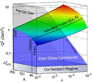
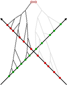
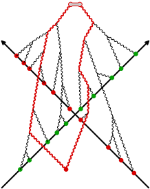
Figure 2: Left: Saturation domain depending on $x$, $Q$ and $A$. From Deshpande et al. (2009). Middle: Connected tree graphs that contribute to the single gluon spectrum at leading order (LO). The red and green dots denote the color sources of the two projectiles. Right: Same at NLO.

Gluons at the edge of saturation dominate scattering processes, allowing a weak coupling treatment for the calculation of the bulk of particle production. However, this system is non-perturbative, since a large occupation number of order $\alpha_{s}^{-1}$ compensates the smallness of the coupling. The Color Glass Condensate (CGC) is a QCD-based effective theory, designed to organize calculations in the saturation regime Gelis et al. (2010). Its central idea is to use the large gluon occupation number in order to organize the expansion around classical solutions.

An observer in the center of momentum frame of a collision sees two streams of color charges flowing from opposite directions, that can be represented as two color currents $J_{1}^{\mu}$ and $J_{2}^{\mu}$. At high energy, their dominant components are the $J^{\pm}$ ($J^{1,2}$ are inversely proportional to the collision energy, and thus neglected). Because of time dilation, the internal dynamics of the projectiles appears totally frozen to the observer, and therefore $J_{1}^{\mu}$ (resp. $J_{2}^{\mu}$) is independent of $x^{+}$ (resp. $x^{-}$):

$$J_{1}^{\mu a}(x)=\delta^{\mu+}\rho_{1a}(x^{-},{\boldsymbol{x}}_{\perp})\quad,\qquad J_{2}^{\mu a}(x)=\delta^{\mu-}\rho_{2a}(x^{+},{\boldsymbol{x}}_{\perp})\;,$$ (1)

where the functions $\rho_{1,2}$ represent the density of color charges in the projectiles. These distributions reflect the configuration of the color charges just before the collision and are not known event-by-event, but one may develop a theory for its statistical distribution $W[\rho]$. The McLerran-Venugopalan McLerran and Venugopalan (1994a, b) model argues that in a nucleus with many colored constituents this distribution should be Gaussian. Moreover, thanks to confinement, this model neglects correlations between partons located at different transverse positions:

$$W[\rho]\equiv\exp\Big{\{}-\int d^{2}{\boldsymbol{x}}_{\perp}\frac{\rho_{a}(x^{-},{\boldsymbol{x}}_{\perp})\rho_{a}(x^{-},{\boldsymbol{x}}_{\perp})}{2\mu^{2}(x^{-},{\boldsymbol{x}}_{\perp})}\Big{\}}\;,$$ (2)

where $\mu^{2}(x^{-},{\boldsymbol{x}}_{\perp})$ characterizes the local density of color charges.

Closer to the observer’s rapidity, degrees of freedom should not be approximated by static sources, but treated as conventional quantum fields. Thus, the CGC is a Yang-Mills theory coupled to an external color current,

$${\cal L}_{{}_{\rm CGC}}\equiv-\frac{1}{2}{\rm tr}\,\big{(}F^{\mu\nu}F_{\mu\nu}\big{)}+J_{\mu}A^{\mu}\;.$$ (3)

The coupling $J_{\mu}A^{\mu}$ is eikonal because the two types of degrees of freedom have vastly different longitudinal momenta. In order to avoid contributions from loop corrections that are already included in the sources, CGC calculations beyond LO require the introduction of cutoffs (one for each projectile) in longitudinal momentum in order to properly separate sources from fields.

The order of magnitude of a connected graph ${\cal G}$ is

$${\cal O}({\cal G})={g}^{-2}g^{n_{{}_{E}}}g^{2n_{{}_{L}}}(gJ)^{n_{{}_{J}}}\;,$$ (4)

where $n_{{}_{E}}$ counts the external gluons, $n_{{}_{L}}$ the independent loops and $n_{{}_{J}}$ the sources $J_{1,2}^{\mu}$ in the graph. In the saturated regime, $gJ\sim g^{0}$, and the order of magnitude depends only on $n_{{}_{E}}$ and $n_{{}_{L}}$. Infinitely many graphs, differing in the number of sources, contribute to a given order in $\alpha_{s}$: despite a weak coupling, the CGC is non-perturbative.

Crucial simplifications occur for inclusive observables, obtained as an average over all final states. In particular, only connected graphs contribute to such observables. The simplest inclusive observable is the single gluon spectrum, obtained at leading order by summing all the tree graphs shown in Fig. 2. These tree graphs can be expressed in terms of a solution to the classical Yang-Mills equations,

$$\big{[}{\cal D}_{\mu},{\cal F}^{\mu\nu}\big{]}=J_{1}^{\nu}+J_{2}^{\nu}\;,\quad\lim_{x^{0}\to-\infty}{\cal A}^{\mu}(x)=0\;,$$ (5)

in the Fock-Schwinger gauge $x^{+}A^{-}+x^{-}A^{+}=0$. Intuitively, the absence of constraints on the gauge field at $x^{0}\to+\infty$ comes from the fact that one sums over all final states.

From this classical solution, the gluon spectrum at LO is given by

$$\left.\frac{d{{{N_{1}}}}}{dYd^{2}\vec{\boldsymbol{p}}_{\perp}}\right|_{{}_{\rm LO}}=\frac{1}{16\pi^{3}}\int_{x,y}\;{e^{ip\cdot(x-y)}}\;\square_{x}\square_{y}\;\sum_{\lambda}\epsilon^{\mu}_{\lambda}\epsilon^{\nu}_{\lambda}\;\;{{\cal A}_{\mu}(x)}{{\cal A}_{\nu}(y)}\;,$$ (6)

where $\square_{x}$ is the D’Alembertian operator and the $\epsilon_{\lambda}^{\mu}$ are polarization vectors. Likewise, the multi-gluon spectra read

$$\left.\frac{d{{{N_{n}}}}}{d^{3}{\boldsymbol{p}}_{1}\cdots d^{3}{\boldsymbol{p}}_{n}}\right|_{{}_{\rm LO}}=\left.\frac{d{{{N_{1}}}}}{d^{3}{\boldsymbol{p}}_{1}}\right|_{{}_{\rm LO}}\times\cdots\times\left.\frac{d{{{N_{1}}}}}{d^{3}{\boldsymbol{p}}_{n}}\right|_{{}_{\rm LO}}\;.$$ (7)

Initial conditions for hydrodynamical models require the energy-momentum tensor, whose expression in terms of the classical chromo-electric and chromo-magnetic fields ${\boldsymbol{E}}^{i}$ and ${\boldsymbol{B}}^{i}$ read

$$T^{00}_{{}_{\rm LO}}=\frac{1}{2}\big{[}{{\boldsymbol{E}}^{2}+{\boldsymbol{B}}^{2}}\big{]}\qquad T^{0i}_{{}_{\rm LO}}=\big{[}{\boldsymbol{E}}\times{\boldsymbol{B}}\big{]}^{i}$$ (8)

$$T^{ij}_{{}_{\rm LO}}=\frac{\delta^{ij}}{2}\big{[}{{\boldsymbol{E}}^{2}+{\boldsymbol{B}}^{2}}\big{]}-\big{[}{\boldsymbol{E}}^{i}{\boldsymbol{E}}^{j}+{\boldsymbol{B}}^{i}{\boldsymbol{B}}^{j}\big{]}\;.$$ (9)

II.2 Practical implementation

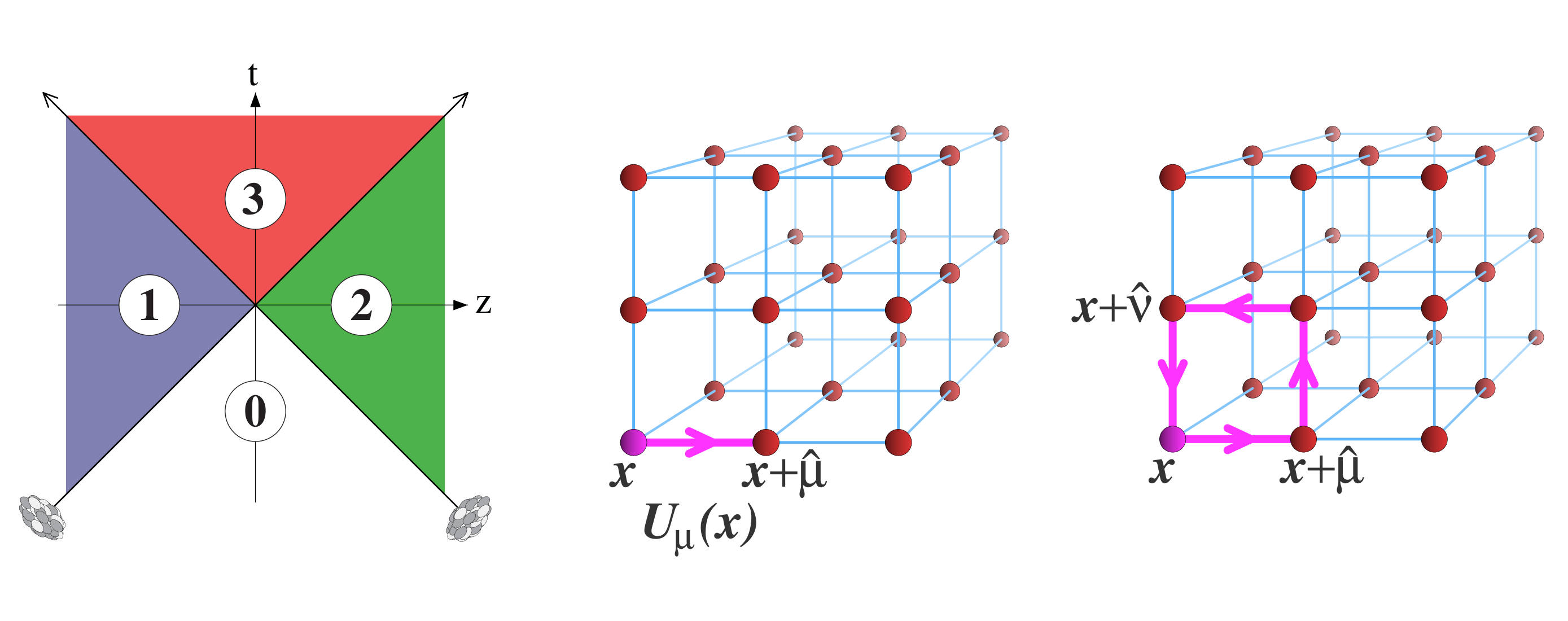
Figure 3: Left: Space-time structure of the classical gauge field ${\cal A}^{\mu}$. Middle and right: Link variable and plaquette on a 3-dimensional lattice.

The non-linear Yang-Mills equations cannot be solved analytically in general. For numerical approaches, one should have in mind the following:

1. Since collisions at high energy are almost invariant under longitudinal boosts, it is natural to map the forward light-cone with proper-time ($\tau\equiv\sqrt{2x^{+}x^{-}}$) and rapidity ($\eta\equiv\frac{1}{2}\log(x^{+}/x^{-})$). The Yang-Mills equations do not depend on rapidity, and become 1+2 dimensional if their initial condition is itself independent of rapidity (which is the case in the CGC at LO).

2. The sources $\rho_{1,2}$ are singular on the light-cones $x^{\pm}=0$, that divide space-time in four regions shown in Fig. 3 (left). The gauge potential ${\cal A}^{\mu}$ vanishes in region 0, and is known analytically in regions 1,2 Kovchegov (1996). In region 3, it is known analytically just above the light-cone, at $\tau=0^{+}$ Kovner et al. (1995) :

   $$A_{0}^{i}=\alpha_{1}^{i}+\alpha_{2}^{i}\quad,\; E_{0}^{i}=0\quad,\;\alpha_{n}^{i}=\frac{i}{g}U_{n}^{\dagger}\partial^{i}U_{n}\quad(n=1,2)\;,$$ (10)

   $$A_{0\eta}=0\quad,\; E_{0}^{\eta}=i\frac{g}{2}[\alpha_{1}^{i},\alpha_{2}^{i}]\;,$$

   where the Wilson line $U_{1}({\boldsymbol{x}}_{\perp})$ reads

   $$V_{1}({\boldsymbol{x}}_{\perp})={\rm P}\,e^{ig\int dx^{-}\frac{1}{\nabla_{\perp}^{2}}\rho_{1}(x^{-},{\boldsymbol{x}}_{\perp})}$$ (11)

   (and a similar expression for $V_{2}$.)

Therefore, one needs to solve numerically 1+2-dim equations for $\tau>0$ Krasnitz and Venugopalan (1999, 2000, 2001); Krasnitz et al. (2001); Krasnitz et al. (2003a); Lappi (2003, 2006); Krasnitz et al. (2003b, c); Lappi and Venugopalan (2006), with initial conditions (10) at $\tau=0^{+}$. In practice, space is discretized on a lattice (see Fig. 3), while time remains a continuously varying variable. One uses Wilson’s formulation, where the gauge potentials $A^{\mu}$ are replaced by link variables (see Fig. 3), i.e. Wilson lines that span one elementary edge of the lattice

$${U_{i}(x)}\equiv{\rm P}\,\exp i\,{g}\int_{x}^{x+\hat{\imath}}ds\;A^{i}(s)\;.$$ (12)

In contrast, the electrical fields $E^{i}$ should be assigned to the nodes of the lattice, and the discretized Hamiltonian reads

$${\cal H} = \sum_{\vec{\boldsymbol{x}};i}\frac{E^{i}({\boldsymbol{x}})E^{i}({\boldsymbol{x}})}{2}$$ (13)

$$-\frac{6}{{g^{2}}}\sum_{\vec{\boldsymbol{x}};ij}1-\frac{1}{3}{\rm Re\ Tr}\,(\underbrace{U_{i}(x)U_{j}(x+\hat{\imath})U^{\dagger}_{i}(x+\hat{\jmath})U^{\dagger}_{j}(x)}_{\mbox{\scriptsize plaquette at the point $\vec{\boldsymbol{x}}$ in the $ij$ plane}})\;.$$

The corresponding Hamilton equations form a large but finite set of ordinary differential equations, that can be solved e.g. by the leapfrog algorithm.

Shortly after the collision (at $\tau\ll Q_{s}^{-1}$), the classical chromo-electric and chromo-magnetic fields are aligned with the collision axis Lappi and McLerran (2006). The expectation value of transverse Wilson loops Dumitru et al. (2013, 2014),

$$W\equiv\left<{\rm P}\,\exp ig\int_{\gamma}dx^{i}{\cal A}^{i}\right>\;,$$ (14)

that measures the magnetic flux through the loop, provides information on the transverse correlation length of these fields. For large loops of area larger than $Q_{s}^{-2}$, $W$ decreases approximately as $\exp(-\#\times\mbox{Area})$, indicating a decorrelation on transverse distances larger than $Q_{s}^{-1}$.

II.3 IP-Glasma framework

As discussed above, Yang-Mills equations for the boost invariant system have to be solved numerically, which has been done for homogeneous nuclei and $N_{c}=2$ in Krasnitz and Venugopalan (1999) and for $N_{c}=3$ in Krasnitz et al. (2001). Finite size nuclei were studied in Krasnitz et al. (2003c); Lappi (2003). In particular, in Krasnitz et al. (2003c) nucleons were sampled from a Woods-Saxon distribution and the color charge density of the nucleus was taken to be proportional to the sum of the thickness functions of all nucleons. Coulomb tails were avoided by implementing a color neutrality condition on length scales given by the inverse of $\Lambda_{\rm QCD}$.

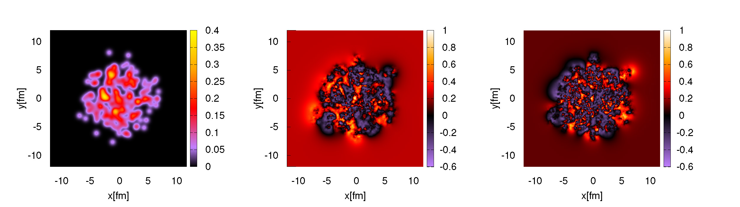
Figure 4: Left: The incoming color charge density $g^{2}\mu^{2}$ for a gold nucleus at $\sqrt{s}=200\,{\rm GeV}$. Middle: The correlator $(1/N_{c}){\rm Re}[{\rm Tr}(V^{\dagger}(0,0)V(x,y))]$ showing the degree of correlations in the gluon fields for a gold ion at $\sqrt{s}=200\,{\rm GeV}$ at an $x$ value that will contribute to gluon production at mid-rapidity. Right: Same as the middle figure but for $\sqrt{s}=5\,{\rm TeV}$.

The IP-Glasma model Schenke et al. (2012a, b) is very similar to the framework introduced in Krasnitz et al. (2003c). The main differences are the use of the IP-Sat model Bartels et al. (2002); Kowalski and Teaney (2003) to constrain the $x$ and transverse position dependence of the color charge density using data from deeply inelastic scattering experiments, and the way one deals with the infrared tails. We now give a brief description of the various steps involved in computing the fluctuating initial state in the IP-Glasma model.

1. Nucleon positions ${\boldsymbol{x}}_{\perp}^{i}$ ($i=1\dots A$) in the transverse plane of two nuclei are sampled from Woods-Saxon distributions with parameters adjusted to the nucleus of interest.

2. The sum of the Gaussian nucleon thickness functions $T_{p}$ is computed. It enters the IP-Sat expression for the dipole cross section in deeply inelastic scattering Kowalski et al. (2008)

   $$\frac{1}{2}\frac{\,\mathrm{d}\sigma^{\textrm{A}}_{\textrm{dip}}}{\,\mathrm{d}^{2}{{\boldsymbol{x}}_{\perp}}}({{\boldsymbol{r}}_{\perp}},{{\boldsymbol{x}}_{\perp}},x)=\mathcal{N}_{A}({{\boldsymbol{r}}_{\perp}},{{\boldsymbol{x}}_{\perp}},x)$$

   $$~{}~{}~{}~{}=\left[1-e^{-\frac{\pi^{2}}{2N_{c}}{\boldsymbol{r}}_{\perp}^{2}\alpha_{s}(Q^{2})xg(x,Q^{2})\sum_{i=1}^{A}T_{p}({{\boldsymbol{x}}_{\perp}}-{\boldsymbol{x}}_{\perp}^{i})}\right]\,.$$ (15)

   $\mathcal{N}_{A}$ is the scattering amplitude of the nucleus, $Q$ is the momentum scale related to the dipole size ${{\boldsymbol{r}}_{\perp}}$, $Q^{2}=4/{\boldsymbol{r}}_{\perp}^{2}+Q_{0}^{2}$, with $Q_{0}$ fixed by the HERA inclusive data. In the first studies Schenke et al. (2012a, b), parameters were taken from the fit in Ref. Kowalski et al. (2006), later Schenke et al. (2014a) parameters from fits to high precision combined data from the H1 and ZEUS collaborations Rezaeian et al. (2013) were used. The gluon distribution $xg(x,Q^{2})$ is parameterized at the initial scale $Q_{0}^{2}$ as $xg(x,Q^{2}_{0})=A_{g}x^{-\lambda_{g}}(1-x)^{5.6}$ and then evolved up to the scale $Q^{2}$ using LO DGLAP-evolution. Like $Q_{0}$, $A_{g}$ and $\lambda_{g}$ are constrained by the fit to HERA data.

3. Using the definition of the nuclear saturation scale $Q_{s}$ as the inverse value of $r=\sqrt{{\boldsymbol{r}}_{\perp}^{2}}$ for which $\mathcal{N}_{A}=1-e^{-1/2}$, $Q_{s}({{\boldsymbol{x}}_{\perp}},x)$ is extracted. Using their proportionality, the color charge squared per unit area $g^{2}\mu^{2}({{\boldsymbol{x}}_{\perp}},x)$ is obtained from $Q_{s}({{\boldsymbol{x}}_{\perp}},x)$. The proportionality factor depends on the details of the calculation Lappi (2008) and in the IP-Glasma calculations it is allowed to be varied in order to reproduce the overall normalization of produced particles Schenke et al. (2012b). A typical distribution of $g^{2}\mu^{2}({{\boldsymbol{x}}_{\perp}})$ is shown in Fig. 4 (left).

4. For a given $x$, which depends on the energy of the collision and the rapidity of interest, color charges $\rho^{a}({{\boldsymbol{x}}_{\perp}})$ are sampled from the distribution (2).

5. Assuming a finite width of the nucleus, the discretized version of the Wilson line (11) is given by Lappi (2008)

   $$V({{\boldsymbol{x}}_{\perp}})=\prod_{k=1}^{N_{y}}\exp\left(-ig\frac{\rho_{k}({{\boldsymbol{x}}_{\perp}})}{\boldsymbol{\nabla}_{\perp}^{2}+m^{2}}\right)\,,$$ (16)

   where $m\sim\Lambda_{\rm QCD}$. The correlator of these Wilson lines $1/N_{c}{\rm Re}[{\rm Tr}(V^{\dagger}(0)V({{\boldsymbol{x}}_{\perp}}))]$ for two nuclei at different energies is shown in Fig. 4 (middle and right). The scale of the fluctuations of this quantity is $1/Q_{s}({{\boldsymbol{x}}_{\perp}})$, which is smaller for the higher energy case (right).

6. For each nucleus an SU($N_{c}$) matrix $V_{j}$ is assigned at each lattice site $j$. They define a pure gauge configuration with the link variables

   $$U^{i}_{j}=V_{j}V^{\dagger}_{j+\hat{e_{i}}}\,,$$ (17)

   where $+\hat{e_{i}}$ indicates a shift from $j$ by one lattice site in the $i=1,2$ direction.

7. The Wilson lines in the future light-cone $U^{i}_{j}$ are determined from those of the two nuclei ($A$ and $B$) by solving

   $${\rm tr}\left\{t^{a}\left[\left(U^{i}_{(A)}+U^{i}_{(B)}\right)(1+U^{i{\dagger}})-(1+U^{i})\left(U^{i{\dagger}}_{(A)}+U^{i{\dagger}}_{(B)}\right)\right]\right\}=0$$ (18)

   iteratively Krasnitz and Venugopalan (1999). Here $t^{a}$ are the generators of $SU(3)$ in the fundamental representation.

8. The lattice expression for the longitudinal electric field can then be obtained from the solutions $U^{i}$ and $U^{i}_{(A,B)}$ Krasnitz and Venugopalan (1999).

9. Given these initial conditions, the source free Yang-Mills equations are solved forward in time (see Section II.2).

From the boost invariant gauge field configurations at finite times one can determine the gluon multiplicity and the energy momentum tensor as a function of transverse position. Employing the proper impact parameter distribution Schenke et al. (2012b) obtained from the Glauber model, the gluon multiplicity distribution can be computed in transverse Coulomb gauge $\partial_{i}A^{i}=0$, $i=1,2$, and compared to the measured charged hadron multiplicity distribution. The result for RHIC energies comparing to uncorrected data from the STAR collaboration is shown in Fig. 5. It was shown Gelis et al. (2009a) that gluons produced from the Glasma naturally follow negative binomial distributions. This can be seen from the distributions for small impact parameter ranges in Fig. 5. It was demonstrated in Schenke et al. (2012a) that these distributions are indeed fit best by negative binomial distributions.

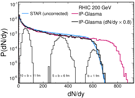
Figure 5: Gluon multiplicity distribution. Shown are also distributions for limited ranges of impact parameter $b$. Experimental data from STAR Abelev et al. (2009). Figure from Schenke et al. (2012b).

II.4 Connection to hydrodynamics and comparison to data

We now discuss how the classical color fields from the IP-Glasma calculation are translated into an initial condition for hydrodynamics, and show comparisons with experimental data for several observables.

The main equations of hydrodynamics are energy and momentum conservation $\partial_{\mu}T^{\mu\nu}=0$ along with an equation of state, where $T^{\mu\nu}$ is the energy momentum tensor. They need to be supplemented by an initial condition for $T^{\mu\nu}$ at some early time, often called the “thermalization time”. The IP-Glasma model provides the gauge field $T^{\mu\nu}$ with one caveat: the gluon field configurations of the IP-Glasma model are not in local equilibrium. In fact, when switching from IP-Glasma dynamics to hydrodynamics at a time of $0.2\,{\rm fm}/c$, the longitudinal pressure of the fields is approximately zero, and negative at earlier times. We will discuss the possibility to reach equilibrium in the Yang-Mills system when including quantum corrections and considering fully three dimensional dynamics below. Lacking a mechanism for equilibration in the 2+1 dimensional LO theory, one way to provide an initial condition for the hydrodynamic equations is to neglect the non-equilibrium components of $T^{\mu\nu}$ and extract the energy density and initial flow velocities by solving the identity $u_{\mu}T^{\mu\nu}=\varepsilon u^{\nu}$ Gale et al. (2013b). There will be discontinuities in other components of $T^{\mu\nu}$ as one switches from the anisotropic field energy momentum tensor to the equilibrium one, which contains the isotropic pressure obtained from the equation of state. However, this should be a good first approximation for matching to fluid dynamics.

Here we will review results for observables that are sensitive to the fluctuations in the initial state of the collision. We will demonstrate that the IP-Glasma model produces fluctuating initial geometries that are consistent with the flow harmonics $v_{n}$ and their event-by-event fluctuations measured at the LHC.

The $v_{n}$ are the coefficients in a Fourier expansion of the azimuthal charged hadron distribution, which is obtained after evolving the hydrodynamic medium and performing a “freeze-out” wherever the system reaches a given minimal temperature or energy density. Every cell, which reaches that threshold, will act like a black body radiator of thermally distributed particles Cooper and Frye (1974). Resonances then decay according to the experimentally observed branching ratios, resulting in the final particle distributions.

II.4.1 Flow harmonics $v_{n}$

Fluid dynamics translates initial geometries into momentum anisotropies, which are quantified by the $v_{n}$. Thus, apart from the right transport properties, a theoretical description must contain the correct initial geometry including event-by-event fluctuations. Fluctuations have a significant effect even on the average values of the $v_{n}$, most notably for odd $n$: Without fluctuating initial conditions the odd harmonics would be zero by symmetry.

The IP-Glasma model in combination with viscous fluid dynamics described above has been shown to lead to an exceptionally good description of all flow harmonics, both as functions of transverse momentum and collision centrality Gale et al. (2013b). This is a non-trivial result because other initial state models could not describe $v_{2}$ and $v_{3}$ simultaneously Qiu et al. (2012). In Fig. 6 we show $v_{n}$ ($n=2,\dots,5$) as functions of $p_{\perp}$ and centrality for Pb+Pb collisions at LHC with a center of mass energy of $\sqrt{s}=2.76\,{\rm TeV}$.

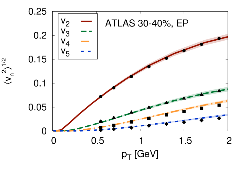
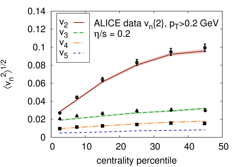
Figure 6: Left: Transverse momentum dependent rms $v_{n}$ compared to ATLAS data Aad et al. (2012). Right: Centrality dependent rms $v_{n}$ compared to ALICE data Aamodt et al. (2011). Figure adapted from Gale et al. (2013b).

II.4.2 $v_{n}$ distributions

An observable that is particularly sensitive to the initial state fluctuations but almost insensitive to the transport properties of the medium is the event-by-event distribution of harmonic flow coefficients Aad et al. (2013); Niemi et al. (2013); Gale et al. (2013b). As discussed in the introduction, several initial state models could be excluded by comparing their predictions for the event-by-event elliptic flow distributions in different centrality classes with experimental data Niemi et al. (2013).

Calculations of scaled event-by-event $v_{n}$ distributions using the IP-Glasma model combined with hydrodynamic evolution are in exceptional agreement with experimental data Gale et al. (2013b); Schenke and Venugopalan (2014). This is demonstrated for 20-25% central events in Fig. 7. For not too peripheral events or too large harmonic number $n$ the initial eccentricity distributions already yield a very good description of the experimental data.

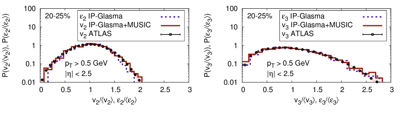
Figure 7: Event-by-event distributions of elliptic (left) and triangular (right) flow coefficients in $\sqrt{s}=2.76\,{\rm TeV}$ collisions at LHC, scaled by the mean values and compared to ATLAS data Aad et al. (2013). Also shown are the scaled initial state eccentricity distributions.

These results indicate that the initial state fluctuations used in the IP-Glasma model describe the experimental reality very well.

II.4.3 Shape-multiplicity correlations in U+U collisions

Another observable that is sensitive to fluctuations and the mechanism of particle production and able to exclude initial state models is the correlation between multiplicity and elliptic flow in ultra-central collisions of deformed nuclei such as uranium U Adamczyk et al. (2015). A Glauber model in which the multiplicity has a significant contribution proportional to the number of binary collisions $N_{\rm bin}$ predicts a strong anti-correlation between $v_{2}$ and the multiplicity in ultra-central U+U collisions. This is because $N_{\rm bin}$ is much larger in the case that the longer axes of both nuclei are aligned with the beam line, than if the shorter axes are.

In contrast, along with a simple constituent quark model, the IP-Glasma model predicts a weaker anti-correlation of the initial geometry with the multiplicity Schenke et al. (2014b), which is very close to the experimental data as demonstrated in Fig. 8.

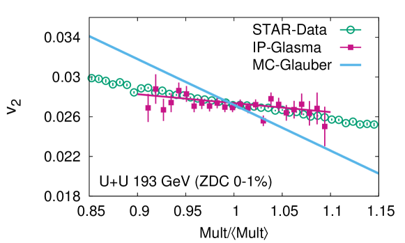
Figure 8: Correlation between $v_{2}$ ($\varepsilon_{2}\langle v_{2}\rangle/\langle\varepsilon_{2}\rangle$ in the theoretical curves) and the scaled multiplicity in 0-1% central U+U events at $\sqrt{s}=193\,{\rm GeV}$. The magenta line is a fit to the IP-Glasma result. Experimental data from STAR Adamczyk et al. (2015).

In the IP-Glasma model the multiplicity is proportional to $Q_{s}^{2}S_{\perp}/\alpha_{s}(Q_{2})$ where $S_{\perp}$ is the transverse size of the overlap region. For tip-tip collisions, which have the smallest $v_{2}$, the increase in $Q_{s}^{2}$ is balanced by a decrease in $S_{\perp}$. $\alpha_{s}$ decreases only logarithmically with increasing $Q_{s}^{2}$ leading to a mildly increased multiplicity in tip-tip collisions compared to body-body collisions (which have the largest $v_{2}$ due to the prolate shape of the U nucleus). The data indicate that effects from sub-nucleonic structure and coherence, as included in the IP-Glasma model, are present and important Adamczyk et al. (2015).

III Quantum fluctuations

III.1 General considerations

The CGC at LO already contains fluctuations of the positions of the nucleons inside a nucleus, and of the distribution of the color charges inside a nucleon. But once the nucleon positions and the color distribution in each nucleon has been chosen, the outcome is deterministic.

At next-to-leading order (NLO), new fluctuations –of quantum origin– appear and the fields are no longer determined deterministically from the color sources. These quantum fluctuations can a priori be of two kinds:

• Initial state fluctuations. Because of the uncertainty principle, the fields and their conjugate momenta cannot be known with arbitrary accuracy. Therefore, a quantum initial state must have fluctuations of the initial values of the fields, in contrast with the CGC at LO. The minimal variance of these fluctuations is controlled by Planck’s constant $\hbar$.

• Quantum “jumps” in the time evolution. In contrast with the LO where Hamilton equations provide unique time derivatives of the fields from their current values, quantum fluctuations also make the evolution non deterministic.

However, NLO corrections (one-loop) are rather special because they only contain quantum fluctuations from the initial state (beyond NLO, fluctuations are both in the initial state and in the evolution). In a quantum system whose classical phase-space is described by coordinates ${\boldsymbol{X}}$ and by momenta ${\boldsymbol{P}}$, the density matrix $\rho_{t}$ evolves according to

$$\partial_{t}\rho_{t}=i\big{[}H,\rho_{t}]\;,$$ (19)

where $H$ is the Hamiltonian operator. A completely equivalent representation is obtained by introducing the Wigner representation,

$${\cal W}_{t}({\boldsymbol{X}},{\boldsymbol{P}}) \equiv \int d{\boldsymbol{s}}\;e^{\tfrac{i}{\hbar}{\boldsymbol{P}}\cdot{\boldsymbol{s}}}\;\big{<}{\boldsymbol{X}}-\tfrac{{\boldsymbol{s}}}{2}\big{|}\rho_{t}\big{|}{\boldsymbol{X}}+\tfrac{{\boldsymbol{s}}}{2}\big{>}$$

$${\cal H}({\boldsymbol{X}},{\boldsymbol{P}}) \equiv \int d{\boldsymbol{s}}\;e^{\tfrac{i}{\hbar}{\boldsymbol{P}}\cdot{\boldsymbol{s}}}\;\big{<}{\boldsymbol{X}}-\tfrac{{\boldsymbol{s}}}{2}\big{|}H\big{|}{\boldsymbol{X}}+\tfrac{{\boldsymbol{s}}}{2}\big{>}\;.$$ (20)

Note that ${\boldsymbol{X}}$ and ${\boldsymbol{P}}$ are commuting classical coordinates, not quantum operators. ${\cal W}_{t}$ is called the Wigner distribution, and ${\cal H}$ is the classical Hamiltonian. ${\cal W}_{t}$ evolves as

$$\partial_{t}{\cal W}_{t}({\boldsymbol{X}},{\boldsymbol{P}}) = \frac{2}{\hbar}{\cal H}({\boldsymbol{X}},{\boldsymbol{P}})\;\sin\left(\frac{\hbar}{2}\left(\stackrel{{\scriptstyle\leftarrow}}{{\nabla}}_{\boldsymbol{X}}\stackrel{{\scriptstyle\rightarrow}}{{\nabla}}_{\boldsymbol{P}}-\stackrel{{\scriptstyle\leftarrow}}{{\nabla}}_{\boldsymbol{P}}\stackrel{{\scriptstyle\rightarrow}}{{\nabla}}_{\boldsymbol{X}}\right)\right)\;{\cal W}_{t}({\boldsymbol{X}},{\boldsymbol{P}})$$ (21)

$$\mathrel{\mathop{\kern 0.0pt\approx}\limits_{\hbar\to 0}} \underbrace{\big{\{}{\cal H},{\cal W}_{t}\big{\}}}_{\mbox{\scriptsize Poisson bracket}}+{\cal O}(\hbar^{2})\;.$$

The first line is exact, and the second line shows the lowest order in $\hbar$. At the order $\hbar^{0}$, we recover classical Hamiltonian dynamics, in the form of the Liouville equation. Remarkably, the first correction arises only at the $\hbar^{2}$ level: at the order $\hbar^{1}$, the time evolution remains classical, and the only quantum effects come from the initial state.

III.2 One loop corrections

Consider now the 1-loop corrections to an observable ${\cal O}(A,\partial A,\cdots)$, that depends on the gauge field operator and its derivatives. One must evaluate graphs such as the one shown in Fig. 2, that contain a loop embedded in the LO classical field Gelis and Venugopalan (2006); Gelis et al. (2007). When its endpoints have a space-like separation, the gluon propagator in a background field reads Gelis et al. (2008a):

$${\cal G}^{\mu a,\nu b}(x,y)\mathrel{\mathop{\kern 0.0pt=}\limits_{(x-y)^{2}\leq 0}}\sum_{\lambda,c}\int\frac{d^{3}{\boldsymbol{k}}}{(2\pi)^{3}2|{\boldsymbol{k}}|}\;a^{\mu a}_{{\boldsymbol{k}}\lambda c}(x)\;a^{\nu b*}_{{\boldsymbol{k}}\lambda c}(y)\;,$$ (22)

where $a_{{\boldsymbol{k}}\lambda c}^{\mu a}(x)$ is a small perturbation obeying the linearized Yang-Mills equations about the classical field ${\cal A}^{\mu}$,

$$\left[{\cal D}_{\mu},\left[{\cal D}^{\mu},a^{\nu}\right]-\left[{\cal D}^{\nu},a^{\mu}\right]\right]-ig\left[{\cal F}^{\nu\mu},a_{\mu}\right]=\hbox{} 0\;, \lim\limits_{t\to-\infty}a^{\mu a}_{{\boldsymbol{k}}\lambda c}(x)=\hbox{} \epsilon^{\mu}_{{\boldsymbol{k}}\lambda}\delta^{a}_{c}\;e^{ik\cdot x}\;.$$ (23)

${\cal D}_{\mu}$ and ${\cal F}^{\mu\nu}$ are the covariant derivative and field strength constructed with the classical field ${\cal A}^{\mu}$. Eq. (22) can also be written as a Gaussian average over random fields,

$${\cal G}^{\mu a,\nu b}(x,y)\mathrel{\mathop{\kern 0.0pt=}\limits_{(x-y)^{2}\leq 0}}\left<A^{\mu a}(x)A^{\nu b}(y)\right>$$ (24)

with

$$A^{\mu a}(x)\equiv\sum_{\lambda,c}\int\frac{d^{3}{\boldsymbol{k}}}{(2\pi)^{3}2|{\boldsymbol{k}}|}\;\Big{[}c_{{\boldsymbol{k}}\lambda c}\,a^{\mu a}_{{\boldsymbol{k}}\lambda c}(x)+\mbox{c.c.}\Big{]}\;,$$

$$\big{<}c_{{\boldsymbol{k}}\lambda c}\big{>}=0\;,\quad\big{<}c_{{\boldsymbol{k}}\lambda c}c_{{\boldsymbol{k}}^{\prime}\lambda^{\prime}c^{\prime}}^{*}\big{>}=\frac{1}{2}\;2\big{|}{\boldsymbol{k}}\big{|}\,(2\pi)^{3}\delta({\boldsymbol{k}}-{\boldsymbol{k}}^{\prime})\,\delta_{\lambda\lambda^{\prime}}\,\delta_{cc^{\prime}}\;.$$ (25)

The fields $A^{\mu a}$ in Eq. (24) are linear superpositions of the $a_{{\boldsymbol{k}}\lambda c}$ with random coefficients that are a classical analogue of creation and annihilation operators. Their variance in Eq. (25) indicates that they correspond to an occupation number $1/2$, that can be interpreted as the zero-point quantum fluctuations in each mode.

Using Eq. (22), the NLO correction to an inclusive observable can be written as follows:

$$\big{<}{\cal O}\big{>}_{{}_{\rm NLO}}=\Bigg{[}\frac{1}{2}\!\!\!\!\int\limits_{{}_{{\boldsymbol{u}},{\boldsymbol{v}}\in\Sigma}}\!\!\!\!\int_{\boldsymbol{k}}\big{[}{a_{\boldsymbol{k}}}\,{\mathbbm{T}}\big{]}_{\boldsymbol{u}}\big{[}{a_{\boldsymbol{k}}^{*}}\,{\mathbbm{T}}\big{]}_{\boldsymbol{v}}+\int\limits_{{}_{{\boldsymbol{u}}\in\Sigma}}\big{[}{{\boldsymbol{\alpha}}}\,{\mathbbm{T}}\big{]}_{\boldsymbol{u}}\Bigg{]}\;\big{<}{\cal O}\big{>}_{{}_{\rm LO}}\;.$$ (26)

In this formula, $\big{<}{\cal O}\big{>}_{{}_{\rm LO}}$ depends on the classical field ${\cal A}^{\mu}$ on a surface $\Sigma$, where the initial value of the classical field is specified, e.g. a surface $\tau={\rm const}$. ${\mathbbm{T}}_{\boldsymbol{u}}$ is the generator of shifts of this initial field: for any function ${\cal F}[{\cal A}_{{}_{\Sigma}}]$ of the fields on $\Sigma$, we have

$$\left[\exp\int_{{\boldsymbol{u}}\in\Sigma}[{\boldsymbol{\alpha}}{\mathbbm{T}}]_{\boldsymbol{u}}\right]\;{\cal F}[{\cal A}_{{}_{\Sigma}}]={\cal F}[{\cal A}_{{}_{\Sigma}}+{\boldsymbol{\alpha}}]\;.$$ (27)

The functions $a_{\boldsymbol{k}}$ in Eq. (26) are the mode functions introduced in Eq. (22) and the function ${\boldsymbol{\alpha}}$ can also be expressed in terms of the same mode functions. Eq. (26) shows that the NLO can be obtained from the LO by fiddling with the initial values of the classical fields, while the fields continue to evolve classically. Note that formulas such as (26) cannot be exact at 2-loops Gelis and Laidet (2013).

III.3 Boost invariant fluctuations and factorization

Some of these fluctuations leads to logarithms of the cutoff that separates the sources from the field degrees of freedom Gelis et al. (2008a, b, 2009b). One can prove that

$$\frac{1}{2}\!\!\!\!\int\limits_{{}_{{\boldsymbol{u}},{\boldsymbol{v}}\in\Sigma}}\!\!\!\!\int_{\boldsymbol{k}}\big{[}{a_{\boldsymbol{k}}}\,{\mathbbm{T}}\big{]}_{\boldsymbol{u}}\big{[}{a_{\boldsymbol{k}}^{*}}\,{\mathbbm{T}}\big{]}_{\boldsymbol{v}}+\int\limits_{{}_{{\boldsymbol{u}}\in\Sigma}}\big{[}{{\boldsymbol{\alpha}}}\,{\mathbbm{T}}\big{]}_{\boldsymbol{u}}=$$

$$\qquad\qquad=\log(\Lambda^{+})\;{\cal H}_{1}+\log(\Lambda^{-})\;{\cal H}_{2}\;+\;\mbox{terms w/o logs}\;,$$ (28)

where the operators ${\cal H}_{1,2}$ are the JIMWLK Hamiltonians of the projectiles Balitsky (1996). The fluctuations that give logarithms of $\Lambda^{+}$ (resp. $\Lambda^{-}$) have a large momentum rapidity in the direction of the nucleus $1$ (resp. nucleus $2$). To the observer, these field fluctuations appear as fast moving color charges, similar the degrees of freedom already included in $\rho_{1,2}$.

Eq. (28) substantiates this intuitive picture. It implies that these logarithms can be absorbed into redefinitions of the distributions $W[\rho_{1,2}]$, evolving with the cutoff according to (Balitsky (1996); Jalilian-Marian et al. (1997a, b, 1998, 1999a, 1999b); Iancu et al. (2001a, b); Ferreiro et al. (2002), see also Balitsky and Chirilli (2008, 2009, 2013); Grabovsky (2013); Kovner et al. (2014a, b, c) for next-to-leading log corrections)

$$\frac{\partial W}{\partial\Lambda}=-{\cal H}\;W\;.$$ (29)

This works because Eq. (28) does not mix $\rho_{1}$ and $\rho_{2}$, a consequence of causality: the logarithms come from soft radiation by fast color charges, which has a long formation time and must occur long before the collision. Therefore, the radiation in nuclei 1 and 2 are independent. All the fluctuation modes that have a rapidity separation $\Delta y\gtrsim\alpha_{s}^{-1}$ with the observer can be resummed in this way, leading to a factorized expression

$$\big{<}{\cal O}\big{>}\mathrel{\mathop{\kern 0.0pt=}\limits_{\mbox{\scriptsize Leading Log}}}\int\big{[}D\rho_{1}\big{]}\big{[}D\rho_{2}\big{]}\;W_{1}[\rho_{1}]\,W_{2}[\rho_{2}]\;{\cal O}_{{}_{\rm LO}}(\rho_{1,2})\;,$$ (30)

where $W_{1}$ and $W_{2}$ are solutions of Eq. (29), starting from an initial condition at the rapidity of the projectile and evolving to the rapidity of the observer. In this new light, the Gaussian distribution introduced in Eq. (2) should be viewed as a model for the initial color distribution, but non-Gaussian correlations may develop when evolving away from the projectile.

Thanks to its structure, the JIMWLK Hamiltonian can be interpreted as a diffusion operator in a functional space, which allows to reproduce the rapidity evolution of $W[\rho]$ by a random walk described by a Langevin equation Blaizot et al. (2003). This approach has been used in several works addressing the numerical study of the JIMWLK equation Rummukainen and Weigert (2004); Dumitru et al. (2011). Note also that, for simple correlators of color charges, this evolution is well described by a mean field approximation known as the Balitsky-Kovchegov equation Kovchegov (1999) (see Balitsky (2007); Balitsky and Chirilli (2008); Kovchegov and Weigert (2007); Gardi et al. (2007) for next-to-leading log corrections).

III.4 Rapidity dependent fluctuations

The fluctuation modes that give logarithms in Eq. (28) preserve the $\eta$-independence of the LO. The remaining modes are $\eta$-dependent, but do not give large logarithms. It is convenient to introduce a new basis:

$$b_{{\boldsymbol{k}}_{\perp}\nu\lambda c}^{\mu a}\equiv\int dy\;e^{i\nu y}\;a_{{\boldsymbol{k}}_{\perp}k_{z}\lambda c}^{\mu a}\;,$$ (31)

where $y$ is the momentum rapidity $y=\ln((k_{0}+k_{z})/(k_{0}-k_{z}))/2$. Since the $a_{{\boldsymbol{k}}\lambda c}({\boldsymbol{x}})$ depend on the momentum and spacetime rapidities only via the difference $y-\eta$, $b_{{\boldsymbol{k}}_{\perp}\nu\lambda c}$ has a trivial rapidity dependence in $\exp(i\nu\eta)$.

The mode functions $b_{{\boldsymbol{k}}\lambda c}$ can be calculated analytically up to a proper time $Q_{s}\tau\ll 1$ Epelbaum and Gelis (2013a) (beyond this time, the classical background field itself is not known analytically), in $A^{\tau}=0$ gauge:

$$b^{ia}_{{\boldsymbol{k}}_{\perp}\nu\lambda c}(\tau,\eta,{\boldsymbol{x}}) = F_{{\boldsymbol{k}}_{\perp}\nu\lambda c}^{+,ia}(\tau,\eta,{\boldsymbol{x}})+F_{{\boldsymbol{k}}_{\perp}\nu\lambda c}^{-,ia}(\tau,\eta,{\boldsymbol{x}})$$

$$b_{{\boldsymbol{k}}_{\perp}\nu\lambda c}^{\eta a}(\tau,\eta,{\boldsymbol{x}}) = {\cal D}^{i}_{ab}\;\Big{(}\frac{F_{{\boldsymbol{k}}_{\perp}\nu\lambda c}^{+,ib}(\tau,\eta,{\boldsymbol{x}})}{2+i\nu}-\frac{F_{{\boldsymbol{k}}_{\perp}\nu\lambda c}^{-,ib}(\tau,\eta,{\boldsymbol{x}})}{2-i\nu}\Big{)}\;,$$

where we denote

$$F_{{\boldsymbol{k}}_{\perp}\nu\lambda c}^{+,ia}(\tau,\eta,{\boldsymbol{x}})\equiv\Gamma(-i\nu)\,e^{+\frac{\nu\pi}{2}}e^{i\nu\eta}\,{V}^{\dagger}_{1ab}({\boldsymbol{x}})\,\vartheta^{j}_{{\bm{k}}\lambda}$$

$$\quad\times\int\frac{d^{2}{\boldsymbol{p}}_{\perp}}{(2\pi)^{2}}\;e^{i{\boldsymbol{p}}\cdot{\boldsymbol{x}}}\;{\widetilde{V}}_{1bc}({\boldsymbol{p}}+{\boldsymbol{k}}_{\perp})\left(\frac{p_{\perp}^{2}\tau}{2k_{\perp}}\right)^{+i\nu}\Big{[}\delta^{ji}-\frac{2p^{j}_{\perp}p^{i}_{\perp}}{p^{2}_{\perp}}\Big{]}$$

$$F_{{\boldsymbol{k}}_{\perp}\nu\lambda c}^{-,ia}(\tau,\eta,{\boldsymbol{x}})\equiv\Gamma(+i\nu)\,e^{-\frac{\nu\pi}{2}}e^{i\nu\eta}\,{V}^{\dagger}_{2ab}({\boldsymbol{x}})\,\vartheta^{j}_{{\bm{k}}\lambda}$$

$$\quad\times\int\frac{d^{2}{\boldsymbol{p}}_{\perp}}{(2\pi)^{2}}\;e^{i{\boldsymbol{p}}\cdot{\boldsymbol{x}}}\;{\widetilde{V}}_{2bc}({\boldsymbol{p}}+{\boldsymbol{k}}_{\perp})\left(\frac{p_{\perp}^{2}\tau}{2k_{\perp}}\right)^{-i\nu}\Big{[}\delta^{ji}-\frac{2p^{j}_{\perp}p^{i}_{\perp}}{p^{2}_{\perp}}\Big{]}$$ (33)

and $\vartheta^{i}_{{\boldsymbol{k}}\lambda}\equiv(\delta^{ij}-2\tfrac{k^{i}k^{j}}{k_{\perp}^{2}})\,\epsilon_{{\boldsymbol{k}}\lambda}^{j}$. The Wilson lines $V_{1,2}$ have been introduced in Eq. (11) (here, they are in the adjoint representation), and the covariant derivative ${\cal D}^{i}_{ab}$ is constructed from the initial field $A_{0}^{i}$ given in Eq. (10). The corresponding electrical fields are obtained by time derivatives of Eqs. (LABEL:eq:finalresult). Since these expressions are only valid at very short proper times, they should be used as initial conditions for Eq. (23).

III.5 Instabilities and classical statistical approximation

After having resummed the large logarithms via the JIMWLK evolution, the remaining contributions are seemingly suppressed by a factor $\alpha_{s}$ compared to LO. However, this conclusion is invalidated by the chaotic behavior of classical solutions of Yang-Mills equations, that are exponentially sensitive to their initial conditions Biro et al. (1994); Heinz et al. (1997); Bolte et al. (2000); Romatschke and Venugopalan (2006a, b, c); Fukushima (2007); Fujii and Itakura (2008); Fujii et al. (2009); Kunihiro et al. (2010); Fukushima and Gelis (2012). Consequently, some of the mode functions $a_{{\boldsymbol{k}}\lambda c}$ grow exponentially with time, and the NLO corrections contain exponentially growing terms: the suppression factor $\alpha_{s}$ quickly becomes irrelevant in view of this time dependence.

The fastest growing can be summed to all orders by exponentiating the quadratic part of the operator that appears in Eq. (26), giving an expression that depends on classical fields averaged over a Gaussian ensemble of fluctuating initial conditions Gelis et al. (2007). This approximation is known as classical statistical approximation (CSA). A strict application of this scheme leads to initial fields that are the sum of the LO classical field ${\cal A}^{\mu}$ (non fluctuating), and a fluctuating part given by Eq. (25) Epelbaum and Gelis (2013b):

$$A^{\mu a}(x)={\cal A}^{\mu a}(x)+\sum_{\lambda,c}\int\frac{d^{3}{\boldsymbol{k}}}{(2\pi)^{3}2|{\boldsymbol{k}}|}\;\Big{[}c_{{\boldsymbol{k}}\lambda c}\,a^{\mu a}_{{\boldsymbol{k}}\lambda c}(x)+\mbox{c.c.}\Big{]}\;,$$

$$\big{<}c_{{\boldsymbol{k}}\lambda c}\big{>}=0\;,\quad\big{<}c_{{\boldsymbol{k}}\lambda c}c_{{\boldsymbol{k}}^{\prime}\lambda^{\prime}c^{\prime}}^{*}\big{>}=\frac{1}{2}\;2\big{|}{\boldsymbol{k}}\big{|}\,(2\pi)^{3}\delta({\boldsymbol{k}}-{\boldsymbol{k}}^{\prime})\,\delta_{\lambda\lambda^{\prime}}\,\delta_{cc^{\prime}}\;.$$ (34)

However, such a spectrum of fluctuations combined with classical time evolution leads to results that are very sensitive to the ultraviolet cutoff Berges et al. (2014a). More formally, this resummation breaks the renormalizability of the underlying theory Epelbaum et al. (2014a, b).

A variant of the CSA uses as initial condition the ensemble of fields corresponding to a classical gas of gluons with a distribution $f({\boldsymbol{k}})$. Such initial fields have no non-fluctuating part, and the variance of the random coefficients is proportional to $f({\boldsymbol{k}})$ Berges et al. (2014b, c, 2015):

$$A^{\mu a}(x)=\sum_{\lambda,c}\int\frac{d^{3}{\boldsymbol{k}}}{(2\pi)^{3}2|{\boldsymbol{k}}|}\;\Big{[}c_{{\boldsymbol{k}}\lambda c}\,a^{\mu a}_{{\boldsymbol{k}}\lambda c}(x)+\mbox{c.c.}\Big{]}\;,$$

$$\big{<}c_{{\boldsymbol{k}}\lambda c}\big{>}=0\;,\quad\big{<}c_{{\boldsymbol{k}}\lambda c}c_{{\boldsymbol{k}}^{\prime}\lambda^{\prime}c^{\prime}}^{*}\big{>}=f({\boldsymbol{k}})\;2\big{|}{\boldsymbol{k}}\big{|}\,(2\pi)^{3}\delta({\boldsymbol{k}}-{\boldsymbol{k}}^{\prime})\,\delta_{\lambda\lambda^{\prime}}\,\delta_{cc^{\prime}}\;.$$ (35)

If $f({\boldsymbol{k}})$ decreases sufficiently fast, this modification leads to ultraviolet finite results.

III.6 Quantum fluctuations in kinetic theory

Eqs. (34) and (35) describe very different systems, despite their similarity:

• The flat spectrum of Eq. (34) on top of a classical field describes a quantum coherent state.

• The compact spectrum of Eq. (35) describes an incoherent classical state (quantum mechanics imposes a minimal variance $1/2$ in all modes).

When applied to simulations of the early stages of heavy ion collisions, these two types of fluctuating initial conditions lead to quite different behaviors of the pressure tensor.

In order to clarify the situation, it would be highly desirable to include quantum fluctuations without sacrificing renormalizability. In field theory, a framework that achieves this is the 2-particle irreducible approximation Luttinger and Ward (1960); Aarts et al. (2002); Calzetta and Hu (2002); Berges (2004, 2005) of the Kadanoff-Baym equations Baym and Kadanoff (1961). Although in principle feasible even for the expanding geometry encountered in heavy ion collisions Hatta and Nishiyama (2012a, b), this is much more complicated to implement than the CSA.

A simpler alternative is to study quantum fluctuations in kinetic theory. Schematically, the Boltzmann equation for $2\to 2$ scatterings reads:

$$\partial_{t}f_{3} \sim g^{4}\int_{124}\cdots\big{[}f_{1}f_{2}({f_{3}+f_{4}})-{f_{3}f_{4}}(f_{1}+f_{2})\big{]}$$ (36)

$$\quad+g^{4}\int_{124}\cdots\big{[}f_{1}f_{2}-{f_{3}f_{4}}\big{]}\;.$$

where the dots encapsulates the cross-section and the delta functions for energy-momentum conservation, whose details are irrelevant here. In Eq. (36), we have written on the first line the terms that correspond to the classical approximation of Eq. (35), and on the second line the terms that come from quantum fluctuations.

Keeping only the cubic terms of the first line may be justified when the occupation number is large. However, this approximation is not uniform over all momentum space, which may be especially problematic in systems with an anisotropic momentum distribution.

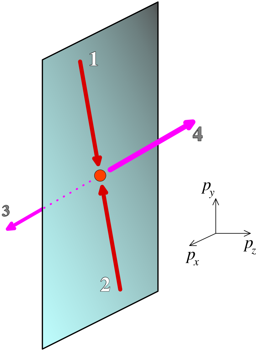
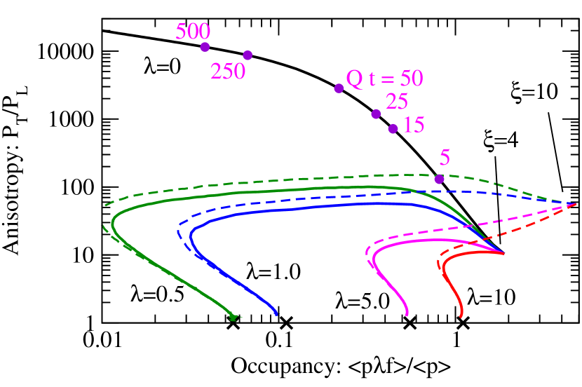
Figure 9: Left: $2\to 2$ scattering contributing to isotropization. Right: time evolution of the anisotropy with the classical ($\lambda=0$) and complete ($\lambda=0.5$ to $10$) Boltzmann equations (plot taken from Kurkela and Zhu (2015), with time labels added by us for clarity).

In the left part of Fig. 9, we illustrate this for a distribution nearly proportional to $\delta(p_{z})$, for which the incoming particles 1,2 have purely transverse momenta. Isotropization requires that at least one of the outgoing particles (3 or 4) has a nonzero $p_{z}$. Nonzero contributions with this kinematics can only come from the second line, which is dropped in the classical approximation.

This has been seen in numerical studies of the Boltzmann equation for a longitudinally expanding system Epelbaum et al. (2015); Kurkela and Zhu (2015). The right part of Fig. 9 shows results with (curves $\lambda=0.5$ to $10$) and without (curve $\lambda=0$) the terms of the second line. Starting at the time $Q\tau=1$ from identical CGC-like initial conditions, the classical and quantum evolutions starts diverging around $Q\tau\approx 2$ for $\lambda=0.5$ (i.e. $\alpha_{s}\approx 0.02$ for $N_{c}=2$ colors), well before the conjectured range of validity of the classical approximation, $Q\tau\approx\alpha_{s}^{-3/2}\approx 350$. These considerations show that quantum fluctuations are essential for isotropization: purely classical approximations do not capture the relevant physics and fail at assessing their own range of validity.

IV Fluctuations in small systems, proton shape

Proton-nucleus collisions, which where initially thought to be an easy to understand reference for heavy ion collisions, have lead to a number of new puzzles since a lot of the collectivity that appears in bigger systems is also visible there. While in nucleus-nucleus collisions, the fluctuations that are internal to a nucleon do not play a big role, because they are averaged over many nucleons, they may become crucial in proton-nucleus collisions.

The fluctuating geometry of a proton will most affect final observables such as anisotropy coefficients $v_{n}$ if final state collective effects are dominant. Hydrodynamic calculations using fluctuating Monte Carlo Glauber initial conditions agree with a variety of experimental observables Bozek (2012); Bozek and Broniowski (2013a); Bozek et al. (2013); Werner et al. (2014a, b); Bozek and Broniowski (2013b); Schenke and Venugopalan (2014); Kozlov et al. (2014). However, more sophisticated models such as the IP-Glasma could not describe the measured $v_{2}$ and $v_{3}$ coefficients in p+Pb collisions Schenke and Venugopalan (2014). The reason for this disagreement was the assumption of a round proton, which was not important for heavy ion collisions. However, in small systems additional sub-nucleonic fluctuations can make a significant difference. For example, the initial color charges in a proton could be concentrated around three valence quarks. It was shown in Schlichting and Schenke (2014) that a proton will retain a memory of the fluctuating shape at large $x$ after JIMWLK evolution over several units in rapidity. This means that a proton at high energy can have fluctuations on various length scales, not just $1/Q_{s}$.

An issue with the use of hydrodynamics in small systems is the possible break-down of its applicability. For small systems the Knudsen number, the ratio of a typical microscopic over a macroscopic scale, can become large, indicating that the hydrodynamic framework is beginning to break down Niemi and Denicol (2014). However, this does not preclude the existence of final state effects, which could be described within a framework other than hydrodynamics.

Apart from the possibility that final state collective effects are dominant also in small collision systems, like p+A, initial state correlations that affect particle production can also contribute to the measured anisotropies Kovner and Lublinsky (2011); Dusling and Venugopalan (2013); Dumitru et al. (2015); Lappi (2015); Lappi et al. (2015). In particular, the classical Yang Mills framework, which is the basis for the IP-Glasma model, contains multi gluon correlations that show qualitatively similar features as the experimental data, namely a relatively large $v_{2}$ and $v_{3}$ in p+A collisions Schenke et al. (2015). Such effects would naturally lead to the observed long range rapidity correlations, which have to be assumed in most hydrodynamic calculations.

At this point it is not yet settled which of the two distinct effects described above dominates the creation of the observed anisotropies. A detailed discussion on the current status of the field can be found in Dusling et al. (2015). Here we conclude that in either case the detailed understanding of sub-nucleonic fluctuations in the initial state is essential for the interpretation of the experimental data of multi particle correlations in small collision systems.

V Conclusions

Fluctuations play a very important role at various levels in the description of heavy ion collisions. Phenomenologically, fluctuations are very important in obtaining the correct final state azimuthal correlations. Their effect is comparatively larger in collisions involving smaller observables, and it is still an open question whether the azimuthal patterns observed in the collision of small systems (p-p collisions) are mostly due to initial state quantum fluctuations.

On a more theoretical level, quantum fluctuations also seem essential in explaining the isotropization of the pressure tensor and the early applicability of hydrodynamics. The complete description of the early time dynamics and transition to the hydrodynamic regime is still an active field of research. Likely the full answer will involve various stages including the unstable evolution in classical Yang-Mills dynamics with quantum corrections and kinetic theory.

References

- Hirano and Tsuda (2002) T. Hirano and K. Tsuda, Phys. Rev. C66, 054905 (2002).
- Kolb and Heinz (2003) P. F. Kolb and U. W. Heinz, Quark Gluon Plasma 3 ed R C Hwa and X N Wang (Singapore: World Scientific) p. 634 (2003), eprint nucl-th/0305084.
- Huovinen (2003) P. Huovinen, Quark Gluon Plasma 3 ed R C Hwa and X N Wang (Singapore: World Scientific) p. 600 (2003), eprint nucl-th/0305064.
- Romatschke and Romatschke (2007) P. Romatschke and U. Romatschke, Phys. Rev. Lett. 99, 172301 (2007).
- Policastro et al. (2001) G. Policastro, D. T. Son, and A. O. Starinets, Phys. Rev. Lett. 87, 081601 (2001), eprint hep-th/0104066.
- Kovtun et al. (2005) P. Kovtun et al., Phys. Rev. Lett. 94, 111601 (2005).
- Schenke et al. (2011) B. Schenke, S. Jeon, and C. Gale, Phys. Rev. Lett. 106, 042301 (2011).
- Bozek and Broniowski (2012) P. Bozek and W. Broniowski, Phys. Rev. C85, 044910 (2012), eprint 1203.1810.
- Karpenko et al. (2015) I. A. Karpenko, P. Huovinen, H. Petersen, and M. Bleicher, Phys. Rev. C91, 064901 (2015).
- Heinz and Snellings (2013) U. Heinz and R. Snellings, Ann. Rev. Nucl. Part. Sci. 63, 123 (2013), eprint 1301.2826.
- Gale et al. (2013a) C. Gale, S. Jeon, and B. Schenke, Int. J. Mod. Phys. A28, 1340011 (2013a), eprint 1301.5893.
- de Souza et al. (2015) R. D. de Souza, T. Koide, and T. Kodama (2015), eprint 1506.03863.
- Jeon and Heinz (2015) S. Jeon and U. Heinz, Int. J. Mod. Phys. E24, 1530010 (2015), eprint 1503.03931.
- Alver et al. (2007) B. Alver et al. (PHOBOS), Phys. Rev. Lett. 98, 242302 (2007), eprint nucl-ex/0610037.
- Mishra et al. (2008) A. P. Mishra, R. K. Mohapatra, P. S. Saumia, and A. M. Srivastava, Phys. Rev. C77, 064902 (2008), eprint 0711.1323.
- Alver and Roland (2010) B. Alver and G. Roland, Phys. Rev. C81, 054905 (2010).
- Alver et al. (2010) B. H. Alver, C. Gombeaud, M. Luzum, and J.-Y. Ollitrault, Phys.Rev. C82, 034913 (2010).
- Aad et al. (2013) G. Aad et al. (ATLAS), JHEP 11, 183 (2013), eprint 1305.2942.
- Niemi et al. (2013) H. Niemi, G. S. Denicol, H. Holopainen, and P. Huovinen, Phys. Rev. C87, 054901 (2013), eprint 1212.1008.
- Schenke et al. (2012a) B. Schenke, P. Tribedy, and R. Venugopalan, Phys. Rev. Lett. 108, 252301 (2012a).
- Schenke et al. (2012b) B. Schenke, P. Tribedy, and R. Venugopalan, Phys. Rev. C86, 034908 (2012b).
- Gale et al. (2013b) C. Gale, S. Jeon, B. Schenke, P. Tribedy, and R. Venugopalan, Phys.Rev.Lett. 110, 012302 (2013b).
- Niemi et al. (2015) H. Niemi, K. J. Eskola, and R. Paatelainen (2015), eprint 1505.02677.
- Moreland et al. (2015) J. S. Moreland, J. E. Bernhard, and S. A. Bass, Phys. Rev. C92, 011901 (2015), eprint 1412.4708.
- Martinez and Strickland (2011) M. Martinez and M. Strickland, Nucl. Phys. A856, 68 (2011), eprint 1011.3056.
- Martinez et al. (2012) M. Martinez, R. Ryblewski, and M. Strickland, Phys. Rev. C85, 064913 (2012), eprint 1204.1473.
- Florkowski et al. (2013) W. Florkowski, R. Ryblewski, and M. Strickland, Nucl. Phys. A916, 249 (2013), eprint 1304.0665.
- Bazow et al. (2014) D. Bazow, U. W. Heinz, and M. Strickland, Phys. Rev. C90, 054910 (2014), eprint 1311.6720.
- Strickland (2014) M. Strickland, Acta Phys. Polon. B45, 2355 (2014), eprint 1410.5786.
- Tinti et al. (2016) L. Tinti, R. Ryblewski, W. Florkowski, and M. Strickland, Nucl. Phys. A946, 29 (2016), eprint 1505.06456.
- Nopoush et al. (2015) M. Nopoush, M. Strickland, R. Ryblewski, D. Bazow, U. Heinz, and M. Martinez, Phys. Rev. C92, 044912 (2015), eprint 1506.05278.
- Heller et al. (2012) M. P. Heller, R. A. Janik, and P. Witaszczyk, Phys. Rev. Lett. 108, 201602 (2012), eprint 1103.3452.
- Kurkela and Zhu (2015) A. Kurkela and Y. Zhu, Phys. Rev. Lett. 115, 182301 (2015), eprint 1506.06647.
- Deshpande et al. (2009) A. Deshpande, R. Ent, and R. Milner, CERN Cour. 49N9, 13 (2009).
- Gelis et al. (2010) F. Gelis, E. Iancu, J. Jalilian-Marian, and R. Venugopalan, Ann. Rev. Nucl. Part. Sci. 60, 463 (2010), eprint 1002.0333.
- McLerran and Venugopalan (1994a) L. D. McLerran and R. Venugopalan, Phys. Rev. D49, 2233 (1994a).
- McLerran and Venugopalan (1994b) L. D. McLerran and R. Venugopalan, Phys. Rev. D49, 3352 (1994b).
- Kovchegov (1996) Y. V. Kovchegov, Phys. Rev. D54, 5463 (1996), eprint hep-ph/9605446.
- Kovner et al. (1995) A. Kovner, L. D. McLerran, and H. Weigert, Phys. Rev. D52, 6231 (1995), eprint hep-ph/9502289.
- Krasnitz and Venugopalan (1999) A. Krasnitz and R. Venugopalan, Nucl. Phys. B557, 237 (1999), eprint hep-ph/9809433.
- Krasnitz and Venugopalan (2000) A. Krasnitz and R. Venugopalan, Phys. Rev. Lett. 84, 4309 (2000).
- Krasnitz and Venugopalan (2001) A. Krasnitz and R. Venugopalan, Phys. Rev. Lett. 86, 1717 (2001).
- Krasnitz et al. (2001) A. Krasnitz, Y. Nara, and R. Venugopalan, Phys. Rev. Lett. 87, 192302 (2001).
- Krasnitz et al. (2003a) A. Krasnitz, Y. Nara, and R. Venugopalan, Nucl. Phys. A727, 427 (2003a).
- Lappi (2003) T. Lappi, Phys. Rev. C67, 054903 (2003).
- Lappi (2006) T. Lappi, Phys. Lett. B643, 11 (2006).
- Krasnitz et al. (2003b) A. Krasnitz, Y. Nara, and R. Venugopalan, Phys. Lett. B554, 21 (2003b).
- Krasnitz et al. (2003c) A. Krasnitz, Y. Nara, and R. Venugopalan, Nucl. Phys. A717, 268 (2003c).
- Lappi and Venugopalan (2006) T. Lappi and R. Venugopalan, Phys. Rev. C74, 054905 (2006).
- Lappi and McLerran (2006) T. Lappi and L. McLerran, Nucl. Phys. A772, 200 (2006), eprint hep-ph/0602189.
- Dumitru et al. (2013) A. Dumitru, Y. Nara, and E. Petreska, Phys. Rev. D88, 054016 (2013), eprint 1302.2064.
- Dumitru et al. (2014) A. Dumitru, T. Lappi, and Y. Nara, Phys. Lett. B734, 7 (2014), eprint 1401.4124.
- Bartels et al. (2002) J. Bartels, K. J. Golec-Biernat, and H. Kowalski, Phys. Rev. D66, 014001 (2002).
- Kowalski and Teaney (2003) H. Kowalski and D. Teaney, Phys. Rev. D68, 114005 (2003).
- Kowalski et al. (2008) H. Kowalski, T. Lappi, and R. Venugopalan, Phys. Rev. Lett. 100, 022303 (2008).
- Kowalski et al. (2006) H. Kowalski, L. Motyka, and G. Watt, Phys. Rev. D74, 074016 (2006).
- Schenke et al. (2014a) B. Schenke, P. Tribedy, and R. Venugopalan, Phys. Rev. C89, 024901 (2014a), eprint 1311.3636.
- Rezaeian et al. (2013) A. H. Rezaeian, M. Siddikov, M. Van de Klundert, and R. Venugopalan, Phys.Rev. D87, 034002 (2013), eprint 1212.2974.
- Lappi (2008) T. Lappi, Eur. Phys. J. C55, 285 (2008).
- Gelis et al. (2009a) F. Gelis, T. Lappi, and L. McLerran, Nucl. Phys. A828, 149 (2009a).
- Abelev et al. (2009) B. I. Abelev et al. (STAR), Phys. Rev. C79, 034909 (2009), eprint 0808.2041.
- Cooper and Frye (1974) F. Cooper and G. Frye, Phys. Rev. D10, 186 (1974).
- Qiu et al. (2012) Z. Qiu, C. Shen, and U. W. Heinz, Phys. Lett. B707, 151 (2012).
- Aad et al. (2012) G. Aad et al. (ATLAS Collaboration), Phys.Rev. C86, 014907 (2012).
- Aamodt et al. (2011) K. Aamodt et al. (ALICE Collaboration), Phys.Rev.Lett. 107, 032301 (2011).
- Schenke and Venugopalan (2014) B. Schenke and R. Venugopalan, Phys.Rev.Lett. 113, 102301 (2014), eprint 1405.3605.
- Adamczyk et al. (2015) L. Adamczyk et al. (STAR), Phys. Rev. Lett. 115, 222301 (2015), eprint 1505.07812.
- Schenke et al. (2014b) B. Schenke, P. Tribedy, and R. Venugopalan, Phys. Rev. C89, 064908 (2014b), eprint 1403.2232.
- Gelis and Venugopalan (2006) F. Gelis and R. Venugopalan, Nucl. Phys. A776, 135 (2006), eprint hep-ph/0601209.
- Gelis et al. (2007) F. Gelis, T. Lappi, and R. Venugopalan, Int. J. Mod. Phys. E16, 2595 (2007), eprint 0708.0047.
- Epelbaum and Gelis (2011) T. Epelbaum and F. Gelis, Nucl. Phys. A872, 210 (2011), eprint 1107.0668.
- Gelis et al. (2008a) F. Gelis, T. Lappi, and R. Venugopalan, Phys. Rev. D78, 054019 (2008a), eprint 0804.2630.
- Gelis and Laidet (2013) F. Gelis and J. u. Laidet, Phys. Rev. D87, 045019 (2013), eprint 1211.1191.
- Gelis et al. (2008b) F. Gelis, T. Lappi, and R. Venugopalan, Phys. Rev. D78, 054020 (2008b), eprint 0807.1306.
- Gelis et al. (2009b) F. Gelis, T. Lappi, and R. Venugopalan, Phys. Rev. D79, 094017 (2009b), eprint 0810.4829.
- Balitsky (1996) I. Balitsky, Nucl. Phys. B463, 99 (1996), eprint hep-ph/9509348.
- Jalilian-Marian et al. (1997a) J. Jalilian-Marian, A. Kovner, L. D. McLerran, and H. Weigert, Phys. Rev. D55, 5414 (1997a), eprint hep-ph/9606337.
- Jalilian-Marian et al. (1997b) J. Jalilian-Marian, A. Kovner, A. Leonidov, and H. Weigert, Nucl. Phys. B504, 415 (1997b), eprint hep-ph/9701284.
- Jalilian-Marian et al. (1998) J. Jalilian-Marian, A. Kovner, A. Leonidov, and H. Weigert, Phys. Rev. D59, 014014 (1998), eprint hep-ph/9706377.
- Jalilian-Marian et al. (1999a) J. Jalilian-Marian, A. Kovner, and H. Weigert, Phys. Rev. D59, 014015 (1999a), eprint hep-ph/9709432.
- Jalilian-Marian et al. (1999b) J. Jalilian-Marian, A. Kovner, A. Leonidov, and H. Weigert, Phys. Rev. D59, 034007 (1999b), [Erratum: Phys. Rev.D59,099903(1999)], eprint hep-ph/9807462.
- Iancu et al. (2001a) E. Iancu, A. Leonidov, and L. D. McLerran, Nucl. Phys. A692, 583 (2001a), eprint hep-ph/0011241.
- Iancu et al. (2001b) E. Iancu, A. Leonidov, and L. D. McLerran, Phys. Lett. B510, 133 (2001b), eprint hep-ph/0102009.
- Ferreiro et al. (2002) E. Ferreiro, E. Iancu, A. Leonidov, and L. McLerran, Nucl. Phys. A703, 489 (2002), eprint hep-ph/0109115.
- Balitsky and Chirilli (2008) I. Balitsky and G. A. Chirilli, Phys. Rev. D77, 014019 (2008), eprint 0710.4330.
- Balitsky and Chirilli (2009) I. Balitsky and G. A. Chirilli, Nucl. Phys. B822, 45 (2009), eprint 0903.5326.
- Balitsky and Chirilli (2013) I. Balitsky and G. A. Chirilli, Phys. Rev. D88, 111501 (2013), eprint 1309.7644.
- Grabovsky (2013) A. V. Grabovsky, JHEP 09, 141 (2013), eprint 1307.5414.
- Kovner et al. (2014a) A. Kovner, M. Lublinsky, and Y. Mulian, Phys. Rev. D89, 061704 (2014a), eprint 1310.0378.
- Kovner et al. (2014b) A. Kovner, M. Lublinsky, and Y. Mulian, JHEP 04, 030 (2014b), eprint 1401.0374.
- Kovner et al. (2014c) A. Kovner, M. Lublinsky, and Y. Mulian, JHEP 08, 114 (2014c), eprint 1405.0418.
- Blaizot et al. (2003) J.-P. Blaizot, E. Iancu, and H. Weigert, Nucl. Phys. A713, 441 (2003), eprint hep-ph/0206279.
- Rummukainen and Weigert (2004) K. Rummukainen and H. Weigert, Nucl. Phys. A739, 183 (2004), eprint hep-ph/0309306.
- Dumitru et al. (2011) A. Dumitru, J. Jalilian-Marian, T. Lappi, B. Schenke, and R. Venugopalan, Phys. Lett. B706, 219 (2011), eprint 1108.4764.
- Kovchegov (1999) Y. V. Kovchegov, Phys. Rev. D60, 034008 (1999), eprint hep-ph/9901281.
- Balitsky (2007) I. Balitsky, Phys. Rev. D75, 014001 (2007), eprint hep-ph/0609105.
- Kovchegov and Weigert (2007) Y. V. Kovchegov and H. Weigert, Nucl. Phys. A784, 188 (2007), eprint hep-ph/0609090.
- Gardi et al. (2007) E. Gardi, J. Kuokkanen, K. Rummukainen, and H. Weigert, Nucl. Phys. A784, 282 (2007), eprint hep-ph/0609087.
- Epelbaum and Gelis (2013a) T. Epelbaum and F. Gelis, Phys. Rev. D88, 085015 (2013a), eprint 1307.1765.
- Mrowczynski (1993) S. Mrowczynski, Phys. Lett. B314, 118 (1993).
- Mrowczynski (1997) S. Mrowczynski, Phys. Lett. B393, 26 (1997), eprint hep-ph/9606442.
- Biro et al. (1994) T. S. Biro, C. Gong, B. Muller, and A. Trayanov, Int. J. Mod. Phys. C5, 113 (1994), eprint nucl-th/9306002.
- Heinz et al. (1997) U. W. Heinz, C. R. Hu, S. Leupold, S. G. Matinyan, and B. Muller, Phys. Rev. D55, 2464 (1997), eprint hep-th/9608181.
- Bolte et al. (2000) J. Bolte, B. Muller, and A. Schafer, Phys. Rev. D61, 054506 (2000), eprint hep-lat/9906037.
- Romatschke and Venugopalan (2006a) P. Romatschke and R. Venugopalan, Phys. Rev. Lett. 96, 062302 (2006a), eprint hep-ph/0510121.
- Romatschke and Venugopalan (2006b) P. Romatschke and R. Venugopalan, Eur. Phys. J. A29, 71 (2006b), eprint hep-ph/0510292.
- Romatschke and Venugopalan (2006c) P. Romatschke and R. Venugopalan, Phys. Rev. D74, 045011 (2006c), eprint hep-ph/0605045.
- Fukushima (2007) K. Fukushima, Phys. Rev. C76, 021902 (2007), [Erratum: Phys. Rev.C77,029901(2007)], eprint 0711.2634.
- Fujii and Itakura (2008) H. Fujii and K. Itakura, Nucl. Phys. A809, 88 (2008), eprint 0803.0410.
- Fujii et al. (2009) H. Fujii, K. Itakura, and A. Iwazaki, Nucl. Phys. A828, 178 (2009), eprint 0903.2930.
- Kunihiro et al. (2010) T. Kunihiro, B. Muller, A. Ohnishi, A. Schafer, T. T. Takahashi, and A. Yamamoto, Phys. Rev. D82, 114015 (2010), eprint 1008.1156.
- Fukushima and Gelis (2012) K. Fukushima and F. Gelis, Nucl. Phys. A874, 108 (2012), eprint 1106.1396.
- Epelbaum and Gelis (2013b) T. Epelbaum and F. Gelis, Phys. Rev. Lett. 111, 232301 (2013b), eprint 1307.2214.
- Berges et al. (2014a) J. Berges, K. Boguslavski, S. Schlichting, and R. Venugopalan, JHEP 05, 054 (2014a), eprint 1312.5216.
- Epelbaum et al. (2014a) T. Epelbaum, F. Gelis, and B. Wu, Phys. Rev. D90, 065029 (2014a), eprint 1402.0115.
- Epelbaum et al. (2014b) T. Epelbaum, F. Gelis, N. Tanji, and B. Wu, Phys. Rev. D90, 125032 (2014b), eprint 1409.0701.
- Berges et al. (2014b) J. Berges, K. Boguslavski, S. Schlichting, and R. Venugopalan, Phys. Rev. D89, 074011 (2014b), eprint 1303.5650.
- Berges et al. (2014c) J. Berges, K. Boguslavski, S. Schlichting, and R. Venugopalan, Phys. Rev. D89, 114007 (2014c), eprint 1311.3005.
- Berges et al. (2015) J. Berges, K. Boguslavski, S. Schlichting, and R. Venugopalan, Phys. Rev. Lett. 114, 061601 (2015), eprint 1408.1670.
- Luttinger and Ward (1960) J. M. Luttinger and J. C. Ward, Phys. Rev. 118, 1417 (1960).
- Aarts et al. (2002) G. Aarts, D. Ahrensmeier, R. Baier, J. Berges, and J. Serreau, Phys. Rev. D66, 045008 (2002), eprint hep-ph/0201308.
- Calzetta and Hu (2002) E. A. Calzetta and B. L. Hu (2002), eprint hep-ph/0205271.
- Berges (2004) J. Berges, Phys. Rev. D70, 105010 (2004), eprint hep-ph/0401172.
- Berges (2005) J. Berges, AIP Conf. Proc. 739, 3 (2005), [,3(2004)], eprint hep-ph/0409233.
- Baym and Kadanoff (1961) G. Baym and L. P. Kadanoff, Phys. Rev. 124, 287 (1961).
- Hatta and Nishiyama (2012a) Y. Hatta and A. Nishiyama, Nucl. Phys. A873, 47 (2012a), eprint 1108.0818.
- Hatta and Nishiyama (2012b) Y. Hatta and A. Nishiyama, Phys. Rev. D86, 076002 (2012b), eprint 1206.4743.
- Epelbaum et al. (2015) T. Epelbaum, F. Gelis, S. Jeon, G. Moore, and B. Wu, JHEP 09, 117 (2015), eprint 1506.05580.
- Bozek (2012) P. Bozek, Phys.Rev. C85, 014911 (2012), eprint 1112.0915.
- Bozek and Broniowski (2013a) P. Bozek and W. Broniowski, Phys.Lett. B718, 1557 (2013a), eprint 1211.0845.
- Bozek et al. (2013) P. Bozek, W. Broniowski, and G. Torrieri, Phys.Rev.Lett. 111, 172303 (2013).
- Werner et al. (2014a) K. Werner, B. Guiot, I. Karpenko, and T. Pierog, Phys. Rev. C89, 064903 (2014a), eprint 1312.1233.
- Werner et al. (2014b) K. Werner, M. Bleicher, B. Guiot, I. Karpenko, and T. Pierog, Phys. Rev. Lett. 112, 232301 (2014b), eprint 1307.4379.
- Bozek and Broniowski (2013b) P. Bozek and W. Broniowski, Phys.Rev. C88, 014903 (2013b), eprint 1304.3044.
- Kozlov et al. (2014) I. Kozlov, M. Luzum, G. Denicol, S. Jeon, and C. Gale (2014), eprint 1405.3976.
- Schlichting and Schenke (2014) S. Schlichting and B. Schenke, Phys.Lett. B739, 313 (2014), eprint 1407.8458.
- Niemi and Denicol (2014) H. Niemi and G. S. Denicol (2014), eprint 1404.7327.
- Kovner and Lublinsky (2011) A. Kovner and M. Lublinsky, Phys. Rev. D83, 034017 (2011), eprint 1012.3398.
- Dusling and Venugopalan (2013) K. Dusling and R. Venugopalan, Phys. Rev. D87, 094034 (2013), eprint 1302.7018.
- Dumitru et al. (2015) A. Dumitru, L. McLerran, and V. Skokov, Phys. Lett. B743, 134 (2015), eprint 1410.4844.
- Lappi (2015) T. Lappi, Phys. Lett. B744, 315 (2015), eprint 1501.05505.
- Lappi et al. (2015) T. Lappi, B. Schenke, S. Schlichting, and R. Venugopalan (2015), eprint 1509.03499.
- Schenke et al. (2015) B. Schenke, S. Schlichting, and R. Venugopalan, Phys. Lett. B747, 76 (2015), eprint 1502.01331.
- Dusling et al. (2015) K. Dusling, W. Li, and B. Schenke (2015), eprint 1509.07939.