Abstract

Pulsar timing arrays are powerful tools to test the existence of cosmic strings by searching for the gravitational wave (GW) background. The amplitude of the background connects to information on cosmic strings such as the tension and string network properties. In addition, one may be able to extract more information on the properties of cosmic strings by measuring anisotropies in the GW background. In this paper, we provide estimates of the level of anisotropy expected in the GW background generated by cusps on cosmic strings. We find that the anisotropy level strongly depends on the initial loop size $\alpha$, and thus we may be able to put constraints on $\alpha$ by measuring the anisotropy of the GW background. We also find that certain regions of the parameter space can be probed by shifting the observation frequency of GWs.

1 Introduction

Cosmic strings are one-dimensional topological defects, which arise naturally in field theories [1, 2], as well as in scenarios of the early Universe based on superstring theory [3, 4, 5]. One promising strategy to test for their existence is to search for gravitational wave (GW) emission from them. In particular, strong GW bursts are emitted from nonsmooth structures such as cusps and kinks [6] and overlapped bursts form a stochastic GW background over a wide range of frequencies [7, 8, 9, 10, 11, 12, 13, 14, 15, 16, 17].

Pulsar timing arrays uniquely probe the GW background at nanohertz frequencies [18, 19, 20, 21]. GWs affect the times of arrival (ToAs) of pulses so that the residuals of the ToAs indicate the existence of GWs. In the case of the stochastic GW background, cross-correlations of the residuals between multiple pulsars are taken to reduce the noise, and the correlation coefficient as a function of the angle between two pulsars is called the Hellings and Downs curve [22]. The current limits on the strain amplitude of the GW background have already produced strong constraints on cosmic strings [18, 20]. In the future, the International Pulsar Timing Array [23] and the Square Kilometre Array (SKA) [24] will enhance the sensitivity and offer the best opportunity to search for cosmic strings.

Recently, a method to analyze anisotropies in the GW background has been progressively developed [25, 26, 27]. The anisotropies can arise due to the finiteness of the GW sources and reflect the number of sources and their distribution. In the presence of anisotropies, the cross-correlation of the timing residuals between different pulsars deviates from that of the Hellings and Downs curve, which is derived assuming an isotropic GW background. Simulation studies have showed that we would obtain substantial evidence for the anisotropy signal when the signal-to-noise ratio is higher than $10$ [28]. The European Pulsar Timing Array [29] reported that the spherical harmonics multipole component of the GW amplitude for $\ell>0$ is less than $40\%$ of the isotropic component with $95\%$ confidence. Although this analysis is developed in the context of a GW background from supermassive black hole (SMBH) binaries, we expect to apply it to the background from cosmic strings as well. Information on the source population would help us to understand the string network evolution.

In this paper, we perform theoretical estimates of the expected level of anisotropy in a GW background composed of a superposition of GW bursts originating from cusps on string loops, which are typically the dominant source of the GW background at nanohertz frequencies. First, we calculate the number density of cosmic string loops as a function of the redshift using the velocity-dependent one-scale model [30, 31] and convert it to the rate of the GW bursts coming to the Earth. Then we generate data sets of GW backgrounds by randomly distributing the burst events in the sky, and calculate the anisotropy level of the GW background using the formalism established in Ref. [28].

This paper is organized as follows: In Sec. 2, we describe the one-scale model to obtain redshift distributions of the loop-number density. Then we present a model to convert the number density to the rate of GW emissions, which we use to construct the data sets of GW backgrounds. In Sec. 3, we briefly present the formalism to estimate a level of anisotropy by decomposing the angular distribution of the GW power on the sky into multipole moments. Then we present the results with the dependence of the initial loop size $\alpha$, which is the key parameter to produce a large anisotropy. Section 4 is devoted to conclusions.

2 GW background from cusps on cosmic string loops

The basic components of a cosmic string network are loops and infinite strings. Loops are continually formed by the intersection of cosmic strings, and the typical loop size at formation is often characterized as $\sim\alpha H(t)^{-1}$, where $H(t)$ is the Hubble scale at loop formation. Estimates in earlier works have suggested that the initial loop size is determined by gravitational backreaction, and $\alpha$ has values smaller than $\sim G\mu$, where $G\mu$ is the tension of cosmic strings [34, 35, 36, 41], while recent simulations suggest that a significant fraction of loops are produced at scales roughly a few orders of magnitude below the horizon size $\alpha\sim O(0.1)$ [37, 38, 39, 40]. Since the loop size distribution is still an ongoing topic [42, 43, 44, 45, 46, 47], we take $\alpha$ as a free parameter, and in fact $\alpha$ is a key parameter for the level of anisotropy.

The other parameters, such as the tension $G\mu$ and reconnection probability $p$, are also important for the evolution of the cosmic string network. The value of the string tension $G\mu$ depends strongly on the generation mechanism. For field-theoretic cosmic strings, $\mu$ is roughly the square of the energy scale of the phase transition which produces cosmic strings. For cosmic superstrings, $\mu$ is determined by the fundamental string scale as well as the warp factor of the extra dimension, and it can take a broad range of values. The tension determines the energy loss of loops through the emission of GWs, and it relates to the lifetime of loops. The value of reconnection probability $p$ also depends on the origin of cosmic strings. It is essentially $1$ for field-theoretic cosmic strings, while it can be smaller than $1$ in the case of cosmic superstrings because of the effect of extra dimensions [48, 49, 50]. Analysis in Ref. [48] suggests the value is in the range of $0.1\leq p\leq 1$ for D-strings and $10^{-3}\leq p\leq 1$ for F-strings. The reduced reconnection probability decreases the loss of infinite string length into loops and eventually enhances the density of the string network [51, 52].

It has been shown that cusps on string loops generically arise once per oscillation time [53] and emit strong GW bursts [6]. The typical frequency of GWs is determined by the loop size at the emission, and so it does depend on $\alpha$. Overlapped GW bursts are detectable as a GW background at nanohertz frequencies when $\alpha$ is not too small [10]. In order to predict the amplitude and anisotropy level of the GW background, we need to estimate the number and amplitude of GW bursts coming to the Earth during the observation period of the pulsar timing arrays. Here, we describe a theoretical model which is used to obtain the number density of loops and to convert it to the GW rate.

2.1 Cosmic string network

Our calculation of the string network evolution is based on the velocity-dependent one-scale model [30, 31]. In this model, the string network of infinite strings is characterized by a correlation length $\xi$, which corresponds to the typical curvature radius and interval of infinite strings. Then the total length $L$ of infinite strings in volume $V$ is given by $L=V/\xi^{2}$, and the average string energy density is given by $\rho=\mu/\xi^{2}$. From the equation of energy conservation, one can obtain an evolution equation for $\rho$, whereas the equations of motion for the Nambu-Goto string yield a equation for the evolution of the typical root mean square velocity $v$ of infinite strings. By defining $\gamma\equiv\xi/t$, the resulting equations are

$$\frac{t}{\gamma}\frac{d\gamma}{dt}=-1+\nu+\frac{\tilde{c}pv}{2\gamma}+\nu v^{2},$$ (1)

$$\frac{dv}{dt}=(1-v^{2})H(\frac{k(v)}{\nu\gamma}-2v),$$ (2)

where $k(v)=\frac{2\sqrt{2}}{\pi}\frac{1-8v^{6}}{1+8v^{6}}$, $H\equiv\dot{a}/a$, and the scale factor $a$ is parametrized as $a(t)\propto t^{\nu}$. The third term on the right-hand side of Eq. (1) represents the loss of energy from infinite strings by the production of loops. The constant parameter $\tilde{c}$ represents the efficiency of loop formation and is set to be $\tilde{c}=0.23$, and the effect of the reconnection probability $p$, which deviates from $1$ for cosmic superstrings, can be simply included by replacing $\tilde{c}$ with $\tilde{c}p$.

Cosmic string networks are known to evolve towards a so-called scaling regime in which the characteristic length of infinite strings $\xi$ evolves at a rate proportional to the Hubble scale and the number of them in a Hubble horizon remains constant. The above sets of equations indeed have asymptotic solutions, which can be obtained by setting $d\gamma/dt$ and $dv/dt$ to be $0$. For example, for $p=1$, we obtain $\gamma_{r}=0.27$ and $\gamma_{m}=0.62$, where $\gamma_{r}$ and $\gamma_{m}$ are the values in the radiation- and matter-dominated eras, respectively. Since the effect of the time dependence of $\gamma$ around the matter-radiation equality is small for the settings in this paper, we approximate $\gamma$ as a step function,

$$\gamma(z)=\begin{cases}\gamma_{r}&;z>z_{\rm eq}\\ \gamma_{m}&;z<z_{\rm eq}\end{cases},$$ (3)

where $z=1/a(t)-1$ represents the redshift and $z_{\rm eq}$ is the redshift at the matter-radiation equality.

In the scaling regime, infinite strings continuously lose their length by formation of loops, and the length to lose in a Hubble volume per Hubble time is comparable to the length of infinite strings in a Hubble volume. Assuming that the size of the loops formed at time $t$ is given by $\alpha t$, the number density of loops generated between time $t$ and $t+dt$ is

$$\frac{dn}{dt}(t)dt=\frac{dt}{\alpha\gamma^{2}t^{4}}.$$ (4)

By taking into account the dilution of the number density due to cosmic expansion $\propto a^{-3}$, the number density of loops formed between $t_{i}$ and $t_{i}+dt_{i}$ at time $t$ is given by

$$\frac{dn}{dt_{i}}(t,t_{i})dt_{i}=\frac{dt_{i}}{\alpha\gamma^{2}t_{i}^{4}}\left(\frac{a(t_{i})}{a(t)}\right)^{3}.$$ (5)

2.2 Rate of GW bursts from cusps on string loops

After loop formation, the loop continues to shrink by emitting energy as GWs and eventually vanishes. The length of a loop at time $t$ formed at $t_{i}$ is written as

$$l(t,t_{i})=\alpha t_{i}-\Gamma G\mu(t-t_{i}),$$ (6)

where $\Gamma$ is a constant which represents the efficiency of GW emission and we take $\Gamma=50$. The Fourier amplitude of a GW burst $\tilde{h}(f)=\int~{}dte^{2\pi ift}h(t)$ from a cusp is formulated in Refs. [6, 7, 8] and given by

$$\tilde{h}(f,z,l)\simeq\frac{G\mu l}{((1+z)fl)^{1/3}r(z)f},$$ (7)

where $r(z)=\int^{z}_{0}dz^{\prime}/H(z^{\prime})$. Using the above two equations, the loop length $l$ and the generation time $t_{i}$ can be given as functions of $\tilde{h}$, $z$, and $f$:

$$t_{i}(f,\tilde{h},z)=\frac{l(f,\tilde{h},z)+\Gamma G\mu t(z)}{\alpha+\Gamma G\mu},$$ (8)

$$l(f,\tilde{h},z)=\left(\frac{\tilde{h}r(z)}{G\mu}(1+z)^{1/3}f^{4/3}\right)^{3/2}.$$ (9)

Cusp formation is expected to occur ${\cal O}(1)$ times in an oscillation period, which is characterized by parameter $c$. The value of $c$ can be made to correspond to the emission efficiency $\Gamma$ [14], and we use $c=2^{1/3}\Gamma/(3\pi^{2})\eqsim 2.13$. Then the number of GWs coming to the Earth per unit time, emitted at redshift between $z$ and $z+dz$ by loops formed between $t_{i}$ and $t_{i}+dt_{i}$, is given using the loop-number density obtained in the previous subsection as

$$\frac{dR}{dzdt_{i}}dzdt_{i}=\frac{1}{4}\theta_{m}(f,z,l)^{2}\frac{2c}{(1+z)l(t(z),t_{i})}\frac{dn}{dt_{i}}(t(z),t_{i})dt_{i}\cdot\frac{dV}{dz}dz\cdot\Theta(2-\theta_{m}(f,z,l)),$$ (10)

where $\theta_{m}$ is the beaming angle of the GW burst and given by

$$\theta_{m}(f,z,l)=((1+z)fl)^{-1/3},$$ (11)

and

$$\frac{dV}{dz}(z)=\frac{4\pi a^{2}(z)r^{2}(z)}{H(z)(1+z)}.$$ (12)

The factor $\frac{1}{4}\theta_{m}(f,z,l)^{2}$ reflects the beaming of the GW bursts, and the Heviside step function $\Theta$ reflects the low-frequency cutoff of $fl\lesssim 2$ at the emission [14]. Using Eqs. (6) and (7), we can rewrite Eq. (10) to express the number of GWs coming per unit time which were emitted at redshift $z$ and which have frequency $f$ and amplitude $\tilde{h}$ at the present time:

$$\frac{dR}{dzd\tilde{h}}(f,\tilde{h},z)=\frac{3}{4}\theta^{2}_{m}(f,z,l)\frac{c}{(1+z)\tilde{h}}\frac{1}{\gamma(t_{i})^{2}\alpha t^{4}_{i}}\frac{1}{\alpha+\Gamma G\mu}\left(\frac{a(t_{i})}{a(t)}\right)^{3}\frac{dV}{dz}\Theta(2-\theta_{m}(f,z,l)).$$ (13)

By integrating the rate along the redshift, we get the total arrival rate of GWs today,

$$\frac{dR}{d\tilde{h}}(f,\tilde{h})=\int^{\infty}_{0}dz\frac{dR}{dzd\tilde{h}}(f,\tilde{h},z).$$ (14)

2.3 GW background

The amplitude of the GW background is characterized by the dimensionless parameter $\Omega_{\rm GW}(f)\equiv(d\rho_{\rm GW}/d\ln f)/\rho_{cr}$, where $\rho_{\rm GW}$ is the energy density of the GWs and $\rho_{cr}$ is the critical density of the Universe. By summing up all the bursts, $\Omega_{\rm GW}$ is given by

$$\Omega_{\rm GW}(f)=\frac{2\pi^{2}}{3H_{0}^{2}}f^{3}\int^{\tilde{h}_{*}}_{0}d\tilde{h}\tilde{h}^{2}\frac{dR}{d\tilde{h}}(f,\tilde{h}),$$ (15)

where $H_{0}=100h$ km/s/Mpc is the Hubble parameter at the present time. The condition of forming a stochastic GW background is commonly implemented by introducing the upper limit of the integration $\tilde{h}_{*}$, which satisfies [9]

$$\int^{\infty}_{\tilde{h}_{*}}d\tilde{h}\frac{dR}{d\tilde{h}}=f.$$ (16)

By setting this, the integration of the GW amplitude is carried out to include only bursts with small $\tilde{h}$ which come to the observer with a time interval shorter than $1/f$. Such bursts overlap each other and are considered to be unresolved as a single burst, while rare bursts with large $\tilde{h}$ are observed individually.

Using the formalisms described above, we show $\Omega_{\rm GW}h^{2}$ as a function of frequency for various values of the initial loop size parameter $\alpha$ in Fig. 1. Figure 2 shows the parameter regions excluded by the current strongest pulsar experiments, as well as regions which can be probed by SKA. For the excluded regions, we use the most stringent limit of the scale-invariant spectrum obtained by NANOGrav [18], $\Omega_{\rm GW}h^{2}<2.2\times 10^{-10}$. And for the SKA-accessible region, we show the region where $\Omega_{\rm GW}h^{2}>10^{-13}$.

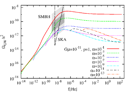
Figure 1: The GW spectra originating from cusps on cosmic string loops are plotted in terms of $\Omega_{\rm GW}h^{2}$ by changing the values of the initial loop size $\alpha$. The cosmic string tension is fixed at $G\mu=10^{-11}$, and the reconnection probability is $p=1$. The sensitivity of the SKA is shown by the black dotted line. The shaded areas represent the 68$\%$ (dark gray) and 99.7$\%$ (light gray) confidence intervals of the theoretically predicted GW amplitude from SMBH binaries according to Ref. [54].

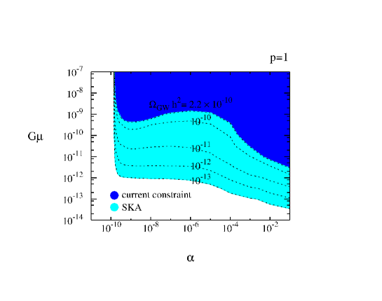
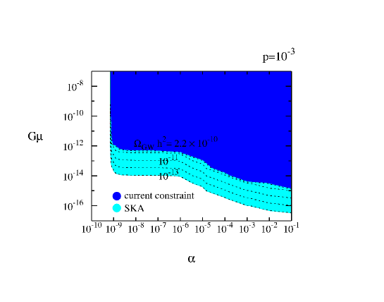
Figure 2: Parameter space accessible by SKA (light blue) for $p=1$ and $p=10^{-3}$. The blue region is the space which is already excluded by the current pulsar constraints. The black dotted lines correspond to contour lines of $\Omega_{\rm GW}h^{2}=10^{-13},10^{-12},10^{-11},10^{-10}$, and $2.2\times 10^{-10}$ from bottom to top.

3 Anisotropies in the GW background

3.1 Method

In order to estimate the anisotropies in the GW background, we simulate the GW background by distributing GW sources on the sky map. First, we compute the GW rate as a function of the amplitude $\tilde{h}$. The GW burst rate for a given amplitude $\tilde{h}$ and for a fixed frequency can be calculated by Eq. (14). Then we distribute GW bursts on the sky according to the obtained burst rate. The position is randomly assigned to each source. We generate 100 realizations of the sky map and calculate the average and variance of the anisotropy level by following the method described in Ref. [28]. The formalism is developed in Ref. [25]. First, we decompose the energy density of GWs $\rho(\hat{\Omega})\propto\tilde{h}^{2}$ in terms of the spherical harmonic functions as

$$\rho(\hat{\Omega})=\sum^{\infty}_{\ell=0}\sum^{\ell}_{m=-\ell}c_{\ell m}Y_{\ell m}(\hat{\Omega}),$$ (17)

where $\hat{\Omega}$ represents the propagation direction of the GW. For point sources, the anisotropy coefficients can be calculated by

$$c_{\ell m}=\sum_{i=1}^{N}\;\rho_{i}Y_{\ell m}(\hat{\Omega}_{i}),$$ (18)

where $\rho_{i}$ describes the GW energy density of each source. Using the definition of the angular power spectrum $C_{\ell}=\sum_{m}|c_{\ell m}|^{2}/(2\ell+1)$, we calculate the anisotropic power normalized by the monopole component $C_{\ell}/C_{0}$.

The above method is identical to decomposing $\Omega_{\rm GW}$ as [25]

$$\Omega_{\rm GW}(f)=\frac{2\pi^{2}}{3H_{0}^{2}}f^{3}\cdot 4H(f)\int d\hat{\Omega}\,P(\hat{\Omega})\,,$$ (19)

with

$$P(\hat{\Omega})=\sum^{\infty}_{\ell=0}\sum^{\ell}_{m=-\ell}\tilde{c}_{\ell m}Y_{\ell m}(\hat{\Omega}).$$ (20)

In this case, the anisotropy coefficients are calculated by

$$\tilde{c}_{\ell m}=\int d\hat{\Omega}\,P(\hat{\Omega})Y_{\ell m}(\hat{\Omega}).$$ (21)

Here, $H(f)$ corresponds to the spectral power of the isotropic (monopole) component, and $P(\hat{\Omega})$ describes the angular distribution of the anisotropic components, which is related to Eq. (15) by $\int d\tilde{h}\tilde{h}^{2}\frac{dR}{d\tilde{h}}=\tilde{h}_{\rm rms}^{2}(f,\hat{\Omega})\equiv 4H(f)\int d\hat{\Omega}P(\hat{\Omega})$. Note that $\tilde{c}_{\ell m}$ is normalized by $\tilde{c}_{00}=\sqrt{4\pi}$, which gives $\int d\hat{\Omega}\,P(\hat{\Omega})=4\pi$, while $c_{\ell m}$ in Eq. (17) includes coefficients of the GW power. This does not make a difference in the results as long as we use the normalized power spectrum $C_{\ell}/C_{0}$.

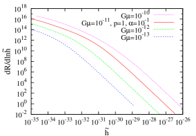
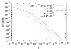
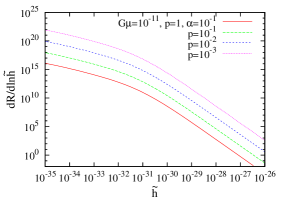
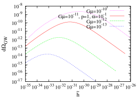
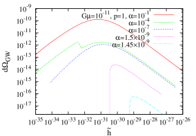
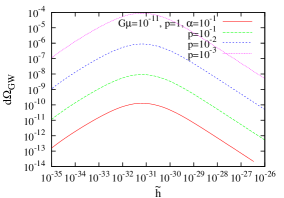
Figure 3: The expected number of GW bursts per logarithmic strain, $dR/d{\ln}\tilde{h}$, for the fixed frequency $f=1/10{\rm years}=3.17\times 10^{-9}{\rm Hz}$. From the left to the right, we show parameter dependencies of $G\mu$, $\alpha$, and $p$. The vertical axis is expected numbers of GW bursts per 10 years.

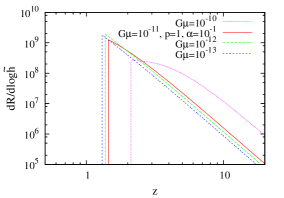
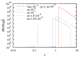
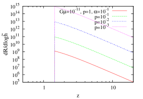
Figure 4: The contribution to the integral of Eq. (15) for each logarithmic strain bin with the same parameter set as in Fig. 5.

Figure 5: The rate shown in terms of the redshift with the same parameter set as in Fig. 5. We fix the strain amplitude to be the one which gives the biggest contribution to the value of $\Omega_{\rm GW}$ (the value of $\tilde{h}$ at the local maximum in Fig. 5).

To calculate the anisotropy coefficients, we use Eq. (18) and sum up all the energy density sources in the simulated sky map. Note that the inclusion of all the sources means that we do not apply the upper limit $\tilde{h}_{*}$ in Eq. (15). This treatment may not be proper when strong bursts are identified and removed from the background data. However, since the observation time of pulsar timing is comparable to the time scale of the GW period $T_{\rm obs}\sim 1/f$, it would be difficult to resolve a single burst, and rare bursts would not be distinguished from the GW background. In fact, the inclusion of $\tilde{h}_{*}$ affects the spectrum shape only at higher frequencies and is important for direct detection by interferometers.

3.2 Rate of GW bursts

Using Eq. (14), we can predict the rate of the GW bursts for a given frequency and given parameter values. Let us first see the parameter dependence of the rate of the GW bursts. Figure 5 shows the GW rate at $f=1/10{\rm years}=3.17\times 10^{-9}{\rm Hz}$ per 10 years for different values of the cosmic string parameters – the tension $G\mu$, the initial loop size $\alpha$, and the reconnection probability $p$. The contribution to $\Omega_{\rm GW}$ is determined by $\tilde{h}^{2}\frac{dR}{d\tilde{h}}$, as seen in Eq. (15). In Fig. 5, we plot the derivative contribution to $\Omega_{\rm GW}$ in terms of $\tilde{h}$ to find the strain amplitude which mainly composes the GW background. In Fig. 5, we show the redshift evolution of the rate using Eq. (13). To calculate the redshift dependence of the rate $\frac{dR}{d\tilde{h}dz}$, we need to fix the value of $\tilde{h}$. We choose $\tilde{h}$ to be the local maximum of each line in Fig. 5 – that is, the value of $\tilde{h}$ which contributes the most to $\Omega_{\rm GW}$.

The small jumps seen in the middle panels of Figs. 5 and 5 for $\alpha=10^{-4}$ are an artifact of the sudden transition of $\gamma$ from the radiation-dominated to the matter-dominated era as provided in Eq. (3). For this low frequency $f=3.17\times 10^{-9}{\rm Hz}$, all GWs are emitted after radiation-matter equality, but the loops are formed in the radiation-dominated era when they have a long lifetime $\alpha=10^{-1}$, while loops are formed in the matter-dominated era when they have a short lifetime $\alpha\leq 10^{-7}$. The intermediate case is $\alpha=10^{-4}$, where GWs with small $\tilde{h}$ are emitted from loops formed during the radiation-dominated era, while a large $\tilde{h}$ corresponds to loops formed in the matter-dominated era.

To achieve the detectable large anisotropy of $\sim\mathcal{O}(10\%)$ in the GW background, a small number of strong bursts should contribute the GW background comparable to the overall amplitude. As seen from Figs. 5 and 5, in most of the cases, the dominant component of the GW background is the numerous small bursts coming from high redshifts, where we cannot expect large anisotropy. The interesting case is found when the initial loop size $\alpha$ is small (see the middle panels). The lifetime of the cosmic string loop is given by the initial energy of the loop divided by the rate of the energy release by GW emissions, $\tau\sim\alpha t_{i}/(\Gamma G\mu)$. Thus, when $\alpha\ll\Gamma G\mu$, loops decay within a Hubble time after their formation. GWs emitted from such short-lived loops have a typical frequency which corresponds to their loop size $(1+z_{i})f\sim 2/(\alpha t_{i})$. Because of this, the GW background of a given frequency consists of GW bursts from a specific redshift, as seen from Fig. 5. For a fixed frequency $f=[\alpha t_{i}(1+z_{i})]^{-1}$, $t_{i}$ should increase for smaller $\alpha$. This leads to a lower number density of loops, since $a(t_{i})^{3}/t_{i}^{4}$ in Eq. (5) is a decreasing function with respect to $t_{i}$. Therefore, as seen in Fig. 5, we find the case where the GW background consists of a small number of bursts for a specific range of $\alpha$. In this case, we can expect a large anisotropy as shown in the next section.

3.3 Results and discussions

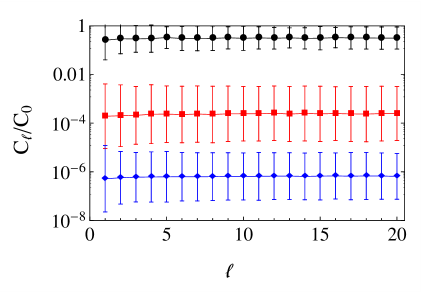
Figure 6: The anisotropy power $C_{\ell}/C_{0}$ for different values of the initial loop size: $\alpha=1.45\times 10^{-9}$ (black), $1.5\times 10^{-9}$ (red), and $10^{-4}$ (blue). We set $G\mu=10^{-11}$ and $p=1$ and assume observation at $f=1/10{\rm year}=3.17\times 10^{-9}{\rm Hz}$.

Finally, we estimate the anisotropy level using the method described in Sec. 3.1. In Fig. 6, we show anisotropy power $C_{\ell}/C_{0}$ up to the multipole $\ell=20$ for $\alpha=1.45\times 10^{-9}$, $1.5\times 10^{-9}$, and $10^{-4}$. The other parameters are fixed at $G\mu=10^{-11}$ and $p=1$. The central point is the mean value of $100$ realizations, and the error bars represent the $2\sigma$ variances. Since we find the distribution is near the log-normal Gaussian distribution, we calculate the mean values and variances for logarithmic values of $C_{\ell}/C_{0}$. We see that the anisotropy becomes large even to a level that could be detected by SKA $\sim\cal{O}$(0.1) in the case of $\alpha=1.45\times 10^{-9}$, but it decreases quickly when $\alpha$ is reduced to $\alpha=1.5\times 10^{-9}$.

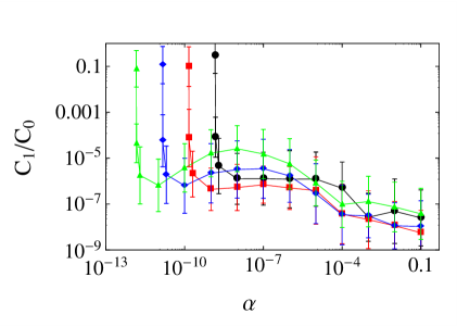
Figure 7: The anisotropy power $C_{\ell}/C_{0}$ of the dipole moment shown as a function of $\alpha$. We assume $G\mu=10^{-11}$ and $p=1$. The different colors describe different observation frequencies; $f=1/10{\rm year}=3.17\times 10^{-9}{\rm Hz}$ (black), $3.17\times 10^{-8}{\rm Hz}$ (red), $3.17\times 10^{-7}{\rm Hz}$ (blue), and $3.17\times 10^{-6}{\rm Hz}$ (green).

Since the anisotropy is the same level for all the multipoles as seen from Fig. 6, let us focus on the dipole moment from now on. In Fig. 7, we plot the dipole power $C_{1}/C_{0}$ as a function of $\alpha$. The different lines correspond to different observation frequency bands. As $\alpha$ decreases, the anisotropy power suddenly increases because of the decrease in the number density of the loops. We do not have points in the region where $\alpha$ is smaller than the peak point, since GWs are not generated in pulsar timing frequencies due to the low-frequency cutoff of the GW emission, $f\lesssim 2/l$. In other words, detecting the strong anisotropy power corresponds to observing the edge of the spectrum at the lowest frequency. As in Fig. 1, the amplitude of the spectrum decreases towards the edge because of the limited number of the loops. The edge shifts to the higher frequency for smaller $\alpha$, and we get no GW power when the spectrum goes out of the sensitivity range of the pulsar timing experiments.

A large anisotropy is achieved only when the GW background consists of bursts from new loops near us without having any contribution from old loops, which are numerous and reduce the anisotropy level. Such conditions are satisfied around the low-frequency cutoff $f\sim 2/(\alpha t_{0})$, which is the typical frequency of bursts from recently formed loops, and old loops cannot contribute to this frequency, since their size must be smaller. Therefore, the position of the anisotropy peak depends on the value of $\alpha$ as well as the observation frequency $f$. For the typical pulsar timing observation frequency $f\sim 1/10$ years, the peak arises at $\alpha\sim 2/(ft_{0})\sim 10^{-9}$. The peak position moves when we change the observation frequency, as seen in Fig. 7.

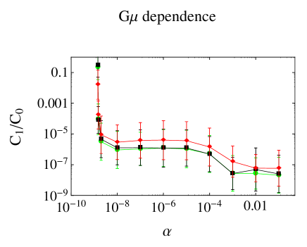
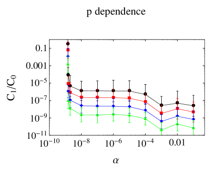
Figure 8: The anisotropy power $C_{\ell}/C_{0}$ of the dipole moment shown as a function of $\alpha$. The observation frequency is assumed to be $f=1/10{\rm year}=3.17\times 10^{-9}{\rm Hz}$. In the left panel, we change the value of tension $G\mu$ by fixing $p=1$; $G\mu=10^{-10}$ (red), $10^{-11}$ (black), and $10^{-12}$ (green). In the right panel, we change the value of reconnection probability by fixing $G\mu=10^{-11}$; $p=1$ (black), $10^{-1}$ (red), $10^{-2}$ (blue), and $10^{-3}$ (green).

In Fig. 8, we show the dependence of our result on other parameters, such as tension $G\mu$ and reconnection probability $p$. We find that the amplitude of the anisotropies changes depending on the parameters, but the position of the peak does not change. The anisotropy amplitude is determined by the number of bursts which form the GW background. We see that the anisotropy is reduced for smaller value of $p$, because small $p$ simply increases the overall amplitude of the number distribution. The value of $G\mu$ changes the number distribution as well as the value of $\tilde{h}$, which gives the main contribution to $\Omega_{\rm GW}$, as seen in Figs. 5 and 5. The combination of the two effects turns out to be a small decrease in the burst number for larger $G\mu$, which is the reason we see the anisotropy gets slightly larger for $G\mu=10^{-10}$. In contrast to the anisotropy amplitude, we find that the peak position does not move for any change of $G\mu$ and $p$. This is because the condition to have a large anisotropy is $f\sim 2/(\alpha t_{0})$, which does not depend on the values of $G\mu$ and $p$.

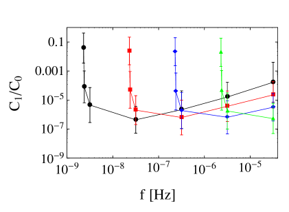
Figure 9: The anisotropy power $C_{\ell}/C_{0}$ of the dipole moment shown as a function of the observation frequency. The different colors describe different values of the initial loop size; $\alpha=10^{-9}$ (black), $10^{-10}$ (red), $10^{-11}$ (blue), and $10^{-12}$ (green). The other parameters are set as $G\mu=10^{-11}$ and $p=1$.

As shown in Fig. 7, one can expect a large anisotropy for different values of $\alpha$ by changing the observation frequency. In Fig. 9, we plot the result as a function of the frequency for different values of $\alpha$. When one analyzes a specific frequency bin, the anisotropy is small for the most of the values of $\alpha$, but one can expect a large anisotropy for a specific value of $\alpha$. This indicates that one can, in principle, test the value of $\alpha$ by checking the anisotropy power at different frequency bands of GWs. A typical GW frequency of the pulsar timing array is $f\sim 1/10{\rm years}=3.17\times 10^{-9}{\rm Hz}$, while we would be able to analyse higher-frequency bands possibly up to $10^{-6}$, which is limited by the monitoring time interval of pulsar observation. Thus, by analyzing frequency bands of $10^{-9}\lesssim f\lesssim 10^{-6}$, we may be able to probe the range of $10^{-11}\lesssim\alpha\lesssim 10^{-9}$.

As for the current constraint, the European Pulsar Timing Array [29] has placed limits on the multipole components of the GW amplitude for $\ell>0$ is less than $40\%$ of the isotropic component at $2-90\times 10^{-9}$Hz. Thus, since the result does not depend on the value of $G\mu$, we can say that $5\times 10^{-11}<\alpha<2\times 10^{-9}$ is excluded for $G\mu\gtrsim 1.3\times 10^{-7}$ with $p=1$ [20]. (Note that we can only exclude the region where the tension is constrained by the multipole component, since the anisotropy level is defined as the ratio to the monopole $C_{\ell}/C_{0}$. ) This corresponds to excluding the left edge of the blue region in Fig. 2.

One may express concern about the assumption of the one-scale model which enforces the uniform initial loop size, while the initial loop size $\alpha$ could be distributed around a typical value. The shape of the GW rate would change when one takes into account the distribution of $\alpha$, but the total number of bursts is important, rather than the shape, for the estimation of the anisotropy level. Thus, we would still find the case where the background consists of a few sources and has a large anisotropy. However, it would be difficult to extract information on the distribution of $\alpha$ from the anisotropy power unless we imposed a simple model for the distribution. This argument would apply also to the case for different models of the cosmic string network. Since the number of bursts is the only key factor for anisotropy, the existence of the strong anisotropy would be universal for most cosmic string models.

Another point we may have to take into account is the relativistic nature of small loops. References [42, 47] pointed out that small loops are created with ultrarelativistic speeds. This would be the case for our targeting range of loop size $10^{-11}\lesssim\alpha\lesssim 10^{-9}$. The relativistic motion of loops would give rise to a blueshift of the GW frequency, which would shift the peak position to large $\alpha$. It would also reduce the beaming angle, and therefore the amplitude of the GW burst would increase while the event rate decreased. This would also affect the peak position, but since these two effects compensate each other, further study is necessary to quantitatively estimate the impact of the relativistic speed of loops on the peak position.

Finally, let us comment on the possibility of testing of the anisotropic GW background by laser-interferometer experiments such as Advanced LIGO [55, 56]. We would expect the same result with a different peak position for LIGO, which is determined by $f_{\rm LIGO}\sim 2/(\alpha t_{0})\sim 100$Hz. An anisotropic background may be rephrased as a noncontinuous background, which is known to be testable by examining the non-Gaussianity of the data. Reference [57] estimates the possibility of detecting such a noncontinuous popcorn-like background from cosmic strings with ground-based laser interferometers. It also estimates the case of pulsar timing frequency $f=10^{-8}$Hz and shows that the popcorn feature arises at $\epsilon\sim 1$ for $G\mu=10^{-11}$, where $\alpha=\epsilon\Gamma G\mu$. This is consistent with our result.

4 Conclusion

We have investigated the possibility of having an anisotropic GW background originating from cosmic string loops. The anisotropy turns out to be too small to be detected by pulsar timing experiments in most parameter spaces, while it becomes large for a specific value of the initial loop size $\alpha$. The large anisotropy is found when a small number of GW bursts contributes to the observed GW background. We found that the parameter space of $\alpha$ yielding a strong anisotropy is very narrow when we analyze the data at a fixed frequency, but one can access $10^{-11}\lesssim\alpha\lesssim 10^{-9}$ by analyzing in different frequency bands.

To have the detectable anisotropy of ${\cal O}(10\%)$, we need the bright outlier source which dominates the overall components of the GW background, as is the same for the SMBH-binary background [28]. The existence of such an outlier may not be extremely rare in the case of SMBH binaries, as some theoretical studies indicate that sources at redshift $0.1-1$ could be bright enough to be individually resolved [58]. On the other hand, in the case of the GW background from cosmic strings, distant sources are typically dominant in number. We have found that the nearest sources become dominant and produce an anisotropic GW background only for the specific parameter choice where the initial loop size $\alpha$ is very small. However, since the properties of the cosmic string network are not understood very well yet, the anisotropy test is still useful for exploring a new parameter space and helps us to understand its distribution.

So far, only the amplitude of the GW background has been used to place constraints on the cosmic string parameters, and the parameter degeneracies cannot be removed only by the information of the amplitude. Although the estimation of the sensitivity for the anisotropy test in multiple frequency bins is beyond our work, anisotropy may provide a new and independent opportunity to constrain the value of $\alpha$ and help to test the string network models.

References

- [1] T. W. B. Kibble, J. Phys. A 9, 1387 (1976).
- [2] A. Vilenkin and E. P. S. Shellard, “Cosmic Strings and Other Topological Defects,” Cambridge University Press, Cambridge, England (1994).
- [3] S. Sarangi and S. H. H. Tye, Phys. Lett. B 536, 185 (2002) [arXiv:hep-th/0204074].
- [4] N. T. Jones, H. Stoica, S. H. H. Tye, Phys. Lett. B563, 6-14 (2003). [hep-th/0303269].
- [5] G. Dvali and A. Vilenkin, JCAP 0403, 010 (2004) [arXiv:hep-th/0312007].
- [6] T. Damour and A. Vilenkin, Phys. Rev. Lett. 85, 3761 (2000) [arXiv:gr-qc/0004075].
- [7] T. Damour and A. Vilenkin, Phys. Rev. D 64, 064008 (2001) [arXiv:gr-qc/0104026].
- [8] T. Damour and A. Vilenkin, Phys. Rev. D 71, 063510 (2005) [arXiv:hep-th/0410222].
- [9] X. Siemens, V. Mandic and J. Creighton, Phys. Rev. Lett. 98, 111101 (2007) [arXiv:astro-ph/0610920].
- [10] M. R. DePies and C. J. Hogan, Phys. Rev. D 75, 125006 (2007) [arXiv:astro-ph/0702335];
- [11] S. Olmez, V. Mandic and X. Siemens, Phys. Rev. D 81, 104028 (2010) doi:10.1103/PhysRevD.81.104028 [arXiv:1004.0890 [astro-ph.CO]].
- [12] S. A. Sanidas, R. A. Battye and B. W. Stappers, Phys. Rev. D 85, 122003 (2012) doi:10.1103/PhysRevD.85.122003 [arXiv:1201.2419 [astro-ph.CO]].
- [13] S. A. Sanidas, R. A. Battye and B. W. Stappers, Astrophys. J. 764, 108 (2013) doi:10.1088/0004-637X/764/1/108 [arXiv:1211.5042 [astro-ph.CO]].
- [14] P. Binetruy, A. Bohe, C. Caprini and J. F. Dufaux, JCAP 1206, 027 (2012) doi:10.1088/1475-7516/2012/06/027 [arXiv:1201.0983 [gr-qc]].
- [15] S. Kuroyanagi, K. Miyamoto, T. Sekiguchi, K. Takahashi and J. Silk, Phys. Rev. D 86, 023503 (2012) [arXiv:1202.3032 [astro-ph.CO]].
- [16] S. Kuroyanagi, K. Miyamoto, T. Sekiguchi, K. Takahashi and J. Silk, Phys. Rev. D 87, no. 2, 023522 (2013) [Phys. Rev. D 87, no. 6, 069903 (2013)] [arXiv:1210.2829 [astro-ph.CO]].
- [17] L. Sousa and P. P. Avelino, Phys. Rev. D 88, no. 2, 023516 (2013) doi:10.1103/PhysRevD.88.023516 [arXiv:1304.2445 [astro-ph.CO]].
- [18] Z. Arzoumanian et al. [NANOGrav Collaboration], Astrophys. J. 821, no. 1, 13 (2016) doi:10.3847/0004-637X/821/1/13 [arXiv:1508.03024 [astro-ph.GA]].
- [19] R. M. Shannon et al., Science 349, no. 6255, 1522 (2015) doi:10.1126/science.aab1910 [arXiv:1509.07320 [astro-ph.CO]].
- [20] L. Lentati et al., Mon. Not. Roy. Astron. Soc. 453, 2576 (2015) doi:10.1093/mnras/stv1538 [arXiv:1504.03692 [astro-ph.CO]].
- [21] J. P. W. Verbiest et al., doi:10.1093/mnras/stw347 arXiv:1602.03640 [astro-ph.IM].
- [22] R. w. Hellings and G. s. Downs, Astrophys. J. 265, L39 (1983). doi:10.1086/183954
- [23] G. Hobbs et al., Class. Quant. Grav. 27, 084013 (2010) doi:10.1088/0264-9381/27/8/084013 [arXiv:0911.5206 [astro-ph.SR]].
- [24] G. Janssen et al., PoS AASKA 14, 037 (2015) [arXiv:1501.00127 [astro-ph.IM]].
- [25] C. M. F. Mingarelli, T. Sidery, I. Mandel and A. Vecchio, Phys. Rev. D 88, no. 6, 062005 (2013) doi:10.1103/PhysRevD.88.062005 [arXiv:1306.5394 [astro-ph.HE]].
- [26] N. J. Cornish and A. Sesana, Class. Quant. Grav. 30, 224005 (2013) doi:10.1088/0264-9381/30/22/224005 [arXiv:1305.0326 [gr-qc]].
- [27] N. J. Cornish and R. van Haasteren, arXiv:1406.4511 [gr-qc].
- [28] S. R. Taylor and J. R. Gair, Phys. Rev. D 88, 084001 (2013) [arXiv:1306.5395 [gr-qc]].
- [29] S. R. Taylor et al. [ Collaboration], Phys. Rev. Lett. 115, no. 4, 041101 (2015) doi:10.1103/PhysRevLett.115.041101 [arXiv:1506.08817 [astro-ph.HE]].
- [30] C. J. A. P. Martins, E. P. S. Shellard, Phys. Rev. D54, 2535-2556 (1996). [arXiv:hep-ph/9602271].
- [31] C. J. A. P. Martins and E. P. S. Shellard, Phys. Rev. D 65, 043514 (2002) doi:10.1103/PhysRevD.65.043514 [hep-ph/0003298].
- [32] M. Kawasaki, K. Miyamoto and K. Nakayama, Phys. Rev. D 81, 103523 (2010) doi:10.1103/PhysRevD.81.103523 [arXiv:1002.0652 [astro-ph.CO]].
- [33] P. Binetruy, A. Bohe, T. Hertog and D. A. Steer, Phys. Rev. D 82, 126007 (2010) doi:10.1103/PhysRevD.82.126007 [arXiv:1009.2484 [hep-th]].
- [34] D. P. Bennett, F. R. Bouchet, Phys. Rev. Lett. 60, 257 (1988), Phys. Rev. Lett. 63, 2776 (1989), Phys. Rev. D41, 2408 (1990).
- [35] B. Allen, E. P. S. Shellard, Phys. Rev. Lett. 64, 119-122 (1990).
- [36] G. R. Vincent, M. Hindmarsh, M. Sakellariadou, Phys. Rev. D56, 637-646 (1997). [astro-ph/9612135].
- [37] V. Vanchurin, K. D. Olum, A. Vilenkin, Phys. Rev. D74, 063527 (2006). [gr-qc/0511159].
- [38] C. Ringeval, M. Sakellariadou, F. Bouchet, JCAP 0702, 023 (2007). [astro-ph/0511646].
- [39] C. J. A. P. Martins, E. P. S. Shellard, Phys. Rev. D73, 043515 (2006). [astro-ph/0511792].
- [40] K. D. Olum, V. Vanchurin, Phys. Rev. D75, 063521 (2007). [astro-ph/0610419].
- [41] X. Siemens, K. D. Olum, A. Vilenkin, Phys. Rev. D66, 043501 (2002). [gr-qc/0203006].
- [42] J. Polchinski, J. V. Rocha, Phys. Rev. D74, 083504 (2006). [hep-ph/0606205].
- [43] F. Dubath, J. Polchinski, J. V. Rocha, Phys. Rev. D77, 123528 (2008). [arXiv:0711.0994 [astro-ph]].
- [44] V. Vanchurin, Phys. Rev. D77, 063532 (2008). [arXiv:0712.2236 [gr-qc]].
- [45] L. Lorenz, C. Ringeval and M. Sakellariadou, JCAP 1010, 003 (2010) [arXiv:1006.0931 [astro-ph.CO]].
- [46] J. J. Blanco-Pillado, K. D. Olum and B. Shlaer, Phys. Rev. D 83, 083514 (2011) doi:10.1103/PhysRevD.83.083514 [arXiv:1101.5173 [astro-ph.CO]].
- [47] J. J. Blanco-Pillado, K. D. Olum and B. Shlaer, Phys. Rev. D 89, no. 2, 023512 (2014) doi:10.1103/PhysRevD.89.023512 [arXiv:1309.6637 [astro-ph.CO]].
- [48] M. G. Jackson, N. T. Jones, J. Polchinski, JHEP 0510, 013 (2005). [hep-th/0405229].
- [49] A. Hanany, K. Hashimoto, JHEP 0506, 021 (2005). [hep-th/0501031].
- [50] M. G. Jackson, JHEP 0709, 035 (2007). [arXiv:0706.1264 [hep-th]].
- [51] M. Sakellariadou, JCAP 0504, 003 (2005). [hep-th/0410234].
- [52] A. Avgoustidis, E. P. S. Shellard, Phys. Rev. D73, 041301 (2006). [astro-ph/0512582].
- [53] T. W. B. Kibble and N. Turok, Phys. Lett. B 116, 141 (1982). doi:10.1016/0370-2693(82)90993-5
- [54] A. Sesana, Mon. Not. Roy. Astron. Soc. 433, 1 (2013) doi:10.1093/mnrasl/slt034 [arXiv:1211.5375 [astro-ph.CO]].
- [55] J. Abadie et al. [LIGO Scientific Collaboration], Phys. Rev. Lett. 107, 271102 (2011) doi:10.1103/PhysRevLett.107.271102 [arXiv:1109.1809 [astro-ph.CO]].
- [56] E. Thrane, S. Ballmer, J. D. Romano, S. Mitra, D. Talukder, S. Bose and V. Mandic, Phys. Rev. D 80, 122002 (2009) doi:10.1103/PhysRevD.80.122002 [arXiv:0910.0858 [astro-ph.IM]].
- [57] T. Regimbau, S. Giampanis, X. Siemens and V. Mandic, Phys. Rev. D 85, 066001 (2012) doi:10.1103/PhysRevD.85.066001, 10.1103/PhysRevD.85.069902 [arXiv:1111.6638 [astro-ph.CO]].
- [58] A. Sesana, A. Vecchio and M. Volonteri, Mon. Not. Roy. Astron. Soc. 394, 2255 (2009) doi:10.1111/j.1365-2966.2009.14499.x [arXiv:0809.3412 [astro-ph]].