A generalized finite element method for linear thermoelasticity
Abstract.
We propose and analyze a generalized finite element method designed for linear quasistatic thermoelastic systems with spatial multiscale coefficients. The method is based on the local orthogonal decomposition technique introduced by Målqvist and Peterseim (Math. Comp., 83(290): 2583–2603, 2014). We prove convergence of optimal order, independent of the derivatives of the coefficients, in the spatial -norm. The theoretical results are confirmed by numerical examples.
1. Introduction
In many applications the expansion and contraction of a material exposed to temperature changes are of great importance. To model this phenomenon a system consisting of an elasticity equation describing the displacement coupled with an equation for the temperature is used, see, e.g., [6]. The full system consists of a hyperbolic elasticity equation coupled with a parabolic equation for the temperature, see [8] for a comprehensive treatment of this formulation. If the inertia effects are negligible, the hyperbolic term in the elasticity equation can be removed. This leads to an elliptic-parabolic system, often referred to as quasistatic. This formulation is discussed in, for instance, [22, 25]. In some settings it is justified to also remove the parabolic term, which leads to an elliptic-elliptic system, see, e.g., [22, 25]. Since the thermoelastic problem is formally equivalent to the system describing poroelasticity, several papers on this equation are also relevant, see, e.g., [5, 24].
In this paper we study the quasistatic case. Existence and uniqueness of a solution to this system are discussed in [22] within the framework of linear degenerate evolution equations in Hilbert spaces. It is also shown that this system is essentially of parabolic type. Existence and uniqueness are also treated in [25] (only two-dimensional problems) and in [23, 21] some results on the thermoelastic contact problem are presented. The classical finite element method for the thermoelastic system is analyzed in [10, 25], where convergence rates of optimal order are derived for problems with solution in or higher.
When the elastic medium of interest is strongly heterogeneous, like composite materials, the coefficients are highly varying and oscillating. Commonly, such coefficients are said to have multiscale features. For these problems classical polynomial finite elements, as in [10, 25], fail to approximate the solution well unless the mesh width resolves the data variations. This is due to the fact that a priori bounds of the error depend on (at least) the spatial -norm of the solution. Since this norm depends on the derivative of the diffusion coefficient, it is of order if the coefficient oscillates with frequency . To overcome this difficulty, several numerical methods have been proposed, see for instance [4, 3, 15, 17, 14].
In this paper we suggest a generalized finite element method based on the techniques introduced in [17], often referred to as local orthogonal decomposition. This method builds on ideas from the variational multiscale method [14, 15], where the solution space is split into a coarse and a fine part. The coarse space is modified such that the basis functions contain information from the diffusion coefficient and have support on small patches. With this approach the basis functions have good approximation properties locally. In [17] the technique is applied to elliptic problems with an arbitrary positive and bounded diffusion coefficient. One of the main advantages is that no assumptions on scale separation or periodicity of the coefficient are needed. Recently, this technique has been applied to several other problems, for instance, semilinear elliptic equations [12], boundary value problems [11], eigenvalue problems [18], linear and semilinear parabolic equations [16], and the linear wave equation [1].
The method we propose in this paper uses generalized finite element spaces similar to those used [17] and [13], together with a correction building on the ideas in [11, 15]. We prove convergence of optimal order that does not depend on the derivatives of the coefficients. We emphasize that by avoiding these derivatives, the a priori bound does not contain any constant of order , although coefficients are highly varying.
In Section 2 we formulate the problem of interest, in Section 3 we first recall the classical finite element method for thermoelasticity and then we define the new generalized finite element method. In Section 4 we perform a localization of the basis functions and in Section 5 we analyze the error. Finally, in Section 6 we present some numerical results.
2. Problem formulation
Let , , be a polygonal/polyhedral domain describing the reference configuration of an elastic body. For a given time we let denote the displacement field and the temperature. To impose Dirichlet and Neumann boundary conditions, we let and denote two disjoint segments of the boundary such that . The segments and are defined similarly.
We use to denote the inner product in and for the corresponding norm. Let denote the classical Sobolev space with norm and let denote the dual space to . Furthermore, we adopt the notation for the Bochner space with the norm
where is a Banach space equipped with the norm . The notation is used to denote . The dependence on the interval and the domain is frequently suppressed and we write, for instance, for . We also define the following subspaces of
Under the assumption that the displacement gradients are small, the (linearized) strain tensor is given by
Assuming further that the material is isotropic, Hooke’s law gives the (total) stress tensor, see e.g. [21] and the references therein,
where is the -dimensional identity matrix, is the thermal expansion coefficient, and and are the so called Lamé coefficients given by
where denotes Young’s elastic modulus and denotes Poisson’s ratio. The materials of interest are strongly heterogeneous which implies that , , and are rapidly varying in space.
The linear quasistatic thermoelastic problem takes the form
| (2.1) | ||||||
| (2.2) | ||||||
| (2.3) | ||||||
| (2.4) | ||||||
| (2.5) | ||||||
| (2.6) | ||||||
| (2.7) |
where is the heat conductivity parameter, which is assumed to be rapidly varying in space.
Remark 2.1.
Assumptions.
We make the following assumptions on the data
-
(A1)
, symmetric,
-
(A2)
, and
Similarly, the constants , and are used to denote the corresponding upper and lower bounds for and .
-
(A3)
, , , and .
To pose a variational form we multiply the equations (2.1) and (2.2) with test functions from and and using Green’s formula together with the boundary conditions (2.3)-(2.6) we arrive at the following weak formulation [10]. Find and , such that,
| (2.8) | ||||||
| (2.9) |
and the initial value is satisfied. Here we use to denote the effective stress tensor and we use to denote the Frobenius inner product of matrices. Using Korn’s inequality we have the following bounds, see, e.g., [7],
| (2.10) |
where (resp. ) depends on (resp. and ). Similarly, there are constants (resp. ) depending on the bound (resp. ) such that
| (2.11) |
Furthermore, we use the following notation for the energy norms induced by the bilinear forms
Existence and uniqueness of a solution to (2.8)-(2.9) have been proved in [22, 25]. There are also some papers on the solution to contact problems, see [2, 23].
Theorem 2.2.
3. Numerical approximation
In this section is we first recall some properties of the classical finite element method for (2.8)-(2.9). In subsection 3.2 we propose a new numerical method built on the ideas from [17]. The localization of this method is treated in Section 4.
3.1. Classical finite element
First, we need to define appropriate finite element spaces. For this purpose we let { be a family of shape regular triangulations of with the mesh size , for . Furthermore, we denote the largest diameter in the triangulation by . We now define the classical piecewise affine finite element spaces
For the discretization in time we consider, for simplicity, a uniform time step such that for and .
Remark 3.1.
The classical linear elasticity equation can in some cases suffer from locking effects when using continuous piecewise linear polynomials in both spaces (P1-P1 elements). These typically occur if is close to (Poisson locking) or if the thickness of the domain is very small (shear locking). In the coupled time-dependent problem locking can occur if is neglected in (2.2) and P1-P1 elements are used. The locking produces artificial oscillations in the numerical approximation of the temperature (or pressure) for early time steps. However, it shall be noted that in the case when is not neglected, this locking effect does not occur, see [20]. Thus, we consider a P1-P1 discretization in this paper.
The classical finite element method with a backward Euler scheme in time reads; for find and , such that
| (3.1) | ||||||
| (3.2) |
where and similarly for . The right hand sides are evaluated at time , that is, and . Given initial data and the system (3.1)-(3.2) is well posed [10]. We assume that is a suitable approximation of . For we note that is uniquely determined by (2.8) at , that is, fulfills the equation
and we thus define to be the solution to
| (3.3) |
The following theorem is a consequence of [10, Theorem 3.1]. The convergence rate is optimal for the two first norms. However, it is not optimal for the -norm . In [10] this is avoided by using second order continuous piecewise polynomials for the displacement (P2-P1 elements). It is, however, noted that the problem is still stable using P1-P1 elements. In this paper we use P1-P1 elements and derive error bounds in the -norm, of optimal order, for both the displacement and the temperature.
Theorem 3.2.
Note that the constant involved in this error bound contains derivatives of the coefficients. Hence, convergence only takes place when the mesh size is sufficiently small (). Throughout this paper, it is assumed that is small enough and and are referred to as reference spaces for the solution. Similarly, and are referred to as reference solutions. In Section 5 this solution is compared with the generalized finite element solution. We emphasize that the generalized finite element solution is computed in spaces of lower dimension and hence not as computationally expensive.
In the following theorem we prove some regularity results for the finite element solution.
Theorem 3.3.
Proof.
From (3.1)-(3.2) and the initial data (3.3) we deduce that the following relation must hold for
| (3.7) | ||||||
| (3.8) |
By choosing and and adding the resulting equations we have
| (3.9) |
Note that the coupling terms cancel. By using Cauchy-Schwarz and Young’s inequality we can bound
Multiplying (3.9) by , summing over , and using (2.10) gives
which is bounded by the right hand side in (3.4).
For the bound (3.5) we note that the following relation must hold for
| (3.10) | ||||||
| (3.11) |
Now choose and and add the resulting equations to get
Multiplying by and using Cauchy-Schwarz and Young’s inequality gives
Summing over and using (2.10) now gives
Here we use summation by parts to get
and can now be kicked to the left hand side.
To estimate and we choose and in (3.7)-(3.8) for . We thus have, since ,
The observation that completes the bound (3.5).
Now assume and and note that the following holds for ,
Choosing , and adding the resulting equations gives
where, again, the coupling terms cancel. The two first terms on the left hand side are positive and can thus be ignored. Multiplying by and gives after using Cauchy-Schwarz and Young’s inequality
Note that , where we use that if . Summing over now gives
To bound the last sum we choose , in (3.10)-(3.11), now with and . Adding the resulting equations gives
Multiplying by and gives after using Cauchy-Schwarz inequality
Summing over and using (2.10) thus gives
To bound the last sum in this estimate we choose , in (3.7)-(3.8) and multiply by to get
Summing over and using (2.11) gives
| (3.12) |
It remains to bound , , and . For this purpose we recall that and use (3.12) for to get
Finally, we have that
and thus (3.6) follows. ∎
3.2. Generalized finite element
In this section we shall derive a generalized finite element method. First we define and analogously to and , but with a larger mesh size . In addition, we assume that the family of triangulations is quasi-uniform and that is a refinement of such that and . Furthermore, we use the notation to denote the free nodes in . The aim is now to define a new (multiscale) space with the same dimension as , but with better approximation properties. For this purpose we define an interpolation operator with the property that and for all
| (3.13) |
where
Since the mesh is assumed to be shape regular, the estimates in (3.13) are also global, i.e.,
| (3.14) |
where is a constant depending on the shape regularity parameter, ;
| (3.15) |
where is the largest ball contained in .
One example of an interpolation that satisfies the above assumptions is , . Here denotes the piecewise -projection onto ( if ), the space of functions that are affine on each triangle . Furthermore, is an averaging operator mapping into , by (coordinate wise)
where . mapping to is defined similarly. For a further discussion on this interpolation and other available options we refer to [19].
Let us now define the kernels of and
The kernels are fine scale spaces in the sense that they contain all features that are not captured by the (coarse) finite element spaces and . Note that the interpolation leads to the splits and , meaning that any function can be uniquely decomposed as , with and , and similarly for .
Now, we introduce a Ritz projection onto the fine scale spaces. For this we use the bilinear forms associated with the diffusion in (2.8)-(2.9). The projection of interest is thus , such that for all , fulfills
| (3.16) | ||||||
| (3.17) |
Note that this is an uncoupled system and and are classical Ritz projections.
For any we have, due to the splits of the spaces and above, that
Using this we define the multiscale spaces
| (3.18) |
Clearly has the same dimension as . Indeed, with denoting the hat function in at node and the hat function in at node , such that
a basis for is given by
| (3.19) |
Finally, we also note that the splits and hold, which fulfill the following orthogonality relation
| (3.20) | ||||||
| (3.21) |
3.2.1. Stationary problem
For the error analysis in Section 5 it is convenient to define the Ritz projection onto the multiscale space using the bilinear form given by the stationary version of (2.8)-(2.9). We thus define , such that for all , fulfills
| (3.22) | ||||||
| (3.23) |
Note that we must have , but in general.
The Ritz projection in (3.22)-(3.23) is upper triangular. Hence, when solving for the term in (3.23) is known. Since this term has multiscale features and appears on the right hand side, we impose a correction on inspired by the ideas in [11] and [15]. The correction is defined as the element , which fulfills
| (3.24) |
and we define .
Note that the Ritz projections are stable in the sense that
| (3.25) |
Remark 3.4.
The problem to find is posed in the entire fine scale space and is thus computationally expensive to solve. The aim is to localize these computations to smaller patches of coarse elements, see Section 4.
To derive error bounds for this projection we define two operators and such that for all we have
| (3.26) | ||||
| (3.27) |
Lemma 3.5.
For all it holds that
| (3.28) | ||||
| (3.29) |
Proof.
It follows from [17] that (3.29) holds, since (3.23) is an elliptic equation of Poisson type. Using an Aubin-Nitsche duality argument as in, e.g., [16], we can derive the following estimate in the -norm
which proves the second inequality in (3.28).
It remains to bound . Recall that any can be decomposed as
where . Using the orthogonality (3.20) and that is a symmetric bilinear form we get
Due to (3.22) and (3.24) we thus have
Define . Using the above relation together with (3.26) we get the bound
Since we have due to (3.13)
where we have used the stability for . The first inequality in (3.28) now follows. ∎
Remark 3.6.
Without the correction the error bound (3.28) would depend on the derivatives of ,
where is large if has multiscale features.
3.2.2. Time-dependent problem
A generalized finite element method with a backward Euler discretization in time is now defined by replacing with and with in (3.1)-(3.2) and adding a correction similar to (3.24). The method thus reads; for find , with , , and , such that
| (3.30) | ||||||
| (3.31) | ||||||
| (3.32) |
where . Furthermore, we define , where is defined by (3.32) for and , such that
| (3.33) |
Proof.
Given , , and , the equations (3.30)-(3.32) yields a square system. Hence, it is sufficient to prove that the solution is unique. Let in (3.30) and in (3.31) and add the resulting equations to get
Using the orthogonality (3.20) and (3.32) this simplifies to
Now, using that is a symmetric bilinear form we get the following identity
| (3.34) | ||||
and using Cauchy-Schwarz and Young’s inequality we derive
This, together with the estimate and (2.10), leads to
Hence, a unique solution exists. ∎
4. Localization
In this section we show how to truncate the basis functions, which is motivated by the exponential decay of (3.19). We consider a localization inspired by the one proposed in [11], which is performed by restricting the fine scale space to patches of coarse elements defined by the following; for
Now let be the restriction of to the patch . We define similarly.
The localized fine scale space can now be used to approximate the fine scale part of the basis functions in (3.19), which significantly reduces the computational cost for these problems. Let denote the inner product over a subdomain and define the local Ritz projection such that for all , fulfills
| (4.1) | ||||||
| (4.2) |
Note that if we replace with in (4.1)-(4.2) and denote the resulting projection , then for all we have
Motivated by this we now define the localized fine scale projection as
| (4.3) |
and the localized multiscale spaces
| (4.4) |
with the corresponding localized basis
| (4.5) |
4.1. Stationary problem
In this section we define a localized version of the stationary problem (3.22)-(3.23). Let , such that for all , . The method now reads; find
and such that
| (4.6) | ||||||
| (4.7) | ||||||
| (4.8) |
Note that the Ritz projection is stable in the sense that
| (4.9) |
The following two lemmas give a bound on the error introduced by the localization.
Lemma 4.1.
For all , there exists , such that
| (4.10) | ||||
| (4.11) | ||||
| (4.12) |
The bounds (4.10)-(4.11) are direct results from [13], while (4.12) follows by a slight modification of the right hand side. We omit the proof here.
The next lemma gives a bound for the localized Ritz projection.
Lemma 4.2.
For all there exist such that
| (4.13) | ||||
| (4.14) |
Proof.
It follows from [11] that (4.14) holds. To prove (4.13) we let and be elements such that
Define . From (4.6)-(4.7) we get have the following identity for any
Using this with we get
Now, using Cauchy-Schwarz and Young’s inequality we get
where the last term is bounded in (4.14). For the first term we get
where the first term on the right hand side is bounded in Lemma 3.5. For the second term we use Lemma 4.1 to get
We can bound this further by using (3.25) and (3.26), such that
Remark 4.3.
To preserve linear convergence, the localization parameter should be chosen such that for some constant . With this choice of we get and we get linear convergence in Lemma 4.2.
4.2. Time-dependent problem
A localized version of (3.30)-(3.32) is now defined by replacing with and with . The method thus reads; for find
and , such that
| (4.16) | ||||||
| (4.17) | ||||||
| (4.18) |
where . Furthermore, we define , where is defined by (4.18) for and such that
| (4.19) |
We also define . Note that for we have due to (3.32)
For the localized version this relation is not true. Instead, we prove the following lemma.
Lemma 4.4.
For , it holds that
Proof.
Note that from (4.18) we have
| (4.20) |
This equation can be viewed as the localization of the following problem. Find , such that
| (4.21) |
Now, [13, Lemma 4.4] gives the bound
where such that
Using this we derive the bound
| (4.22) | ||||
Now, to prove the lemma we use (4.21) and Cauchy-Schwarz inequality to get
Applying (4.22) finishes the proof.
∎
The proof can be modified slightly to show the following bound
| (4.23) |
Also note that it follows, by choosing and respectively, that
| (4.24) |
Assumptions.
Proof.
This proof is similar the proof of Lemma 3.7, but we need to account for the lack of orthogonality and the fact that (3.32) is not satisfied.
Given , , and , the equations (4.16)-(4.18) yields a square system, so it is sufficient to prove that the solution is unique. Choosing in (4.16) and in (4.17) and adding the resulting equations we get
Now, using (3.34) and
together with the estimate , gives
Using Lemma 4.4 we have
and the almost orthogonal property (4.15) gives
Now, using that should be chosen such that linear convergence is obtained, see Remark 4.3, that is , we conclude after using Young’s inequality that
where assumption (A4) guarantees that the coefficients are positive. Hence, a unique solution exists. ∎
5. Error analysis
In this section we analyze the error of the generalized finite element method. The results are based on assumption (A4). In the analysis we utilize the following property, which is similar to Lemma 4.4.
Lemma 5.1.
Let and . Then, for , it holds that
Proof.
The proof is similar to the proof of Lemma 4.4. We omit the details. ∎
This can be modified slightly to show the following bound
| (5.1) |
Also note that it follows, by choosing and respectively, that
| (5.2) |
Theorem 5.2.
The proof of Theorem 5.2 is based on two lemmas.
Lemma 5.3.
Proof.
We divide the error into the terms
We also adopt the following notation
From (3.2) it follows that
so by Lemma 4.2 we have the bound
where denotes the -projection onto . Theorem 3.3 now completes this bound. Similarly, (3.1) gives
so, again, by Lemma 4.2 we get
which can be further bounded by using Theorem 3.3. To bound and we note that for
| (5.3) | ||||
where we have used the Ritz projection (4.6), and the equations (3.1) and (4.16). Similarly, for we have
For simplicity, we denote such that
| (5.4) |
Now, choose and and add the resulting equations. Note that the coupling terms on the left hand side results in the term . We conclude that
and by splitting the first term
| (5.5) | ||||
Using Lemma 5.1 we can bound
| (5.6) | ||||
and the almost orthogonal property (4.15) together with (5.2) gives
| (5.7) |
Thus, multiplying (5.5) by and using Cauchy-Schwarz and Young’s inequality we get
where can be kicked to the left hand side. Summing over gives
where we have used that . Furthermore, we note that if , then and . Hence, . From (4.19) and (3.3) we have, if , for ,
so also .
To bound and we note that due to (3.1) and (3.3), and satisfy the equation
Hence, by Lemma 4.2 and the Aubin-Nitsche duality argument we have
| (5.8) |
and for we get
| (5.9) | ||||
Thus, using (2.10), we arrive at the following bound
| (5.10) | ||||
where we apply Theorem 3.3 to the first sum on the right hand side. If we can find an upper bound on , then (5.10) gives a bound for . This is done next, and we bound at the same time. For this purpose, we choose in (5.4) and note that it follows from (5.3) that
| (5.11) |
This also holds for since and . Thus, by adding the resulting equations, we have
where we have used (4.15). For the last term we use Lemma 5.1 to achieve
Thus, we have
and using Young’s inequality we deduce
where assumption (A4) guarantees that the coefficients are positive. Multiplying by , using that , and summing over we derive
where we have used that , the bound (2.11), and (5.8)-(5.9). We can now apply Theorem 3.3. Thus, the lemma follows for . Moreover, this bounds the last terms in (5.10), which completes the proof. ∎
Lemma 5.4.
Proof.
As in the proof of Lemma 5.3 we split the error into two parts
where Lemma 4.2 and Theorem 3.3 gives
Now, note that (5.4) and (5.11) holds also when and . In particular, (5.11) holds also for due to the definition of and in (4.19) and (3.3) respectively. By choosing and adding the resulting equations we derive
Recall . As in the proof of Lemma 5.3 we get from Lemma 5.2
and from (4.15)
Hence, we have
and assumption (A4) guarantees that the coefficients are positive. Multiplying by , using that and , for , now give
Note that this inequality also holds for , since (recall ). Summing over gives and using (2.11)
| (5.13) | ||||
and since and , Lemma 4.2 and the Aubin-Nitsche trick as in (5.8) together with Theorem 3.3 give
| (5.14) | ||||
To bound the last sum on the right hand side in (5.13) we choose and in (5.4) and (5.3) and add the resulting equations. This gives
where the use of (5.6) and (5.7) gives
Multiplying by and using that we get
where we have used Young’s (weighted) inequality on the form, , in the last step. For the second term we have used the inequality with an additional , i.e. . Note that can be made arbitrarily small. Summing over and using (2.10) now gives
| (5.15) | ||||
We can now use (5.13) to deduce
Using this in (5.15) gives
| (5.16) | ||||
Since now can be made arbitrarily small the term can be moved to the left hand side. To estimate the last sum on the right hand side in (5.16) we multiply (5.4) by and sum over to get
| (5.17) |
where we note that and . By choosing in (5.3) and in (5.17) and adding the resulting equations we get
where we have used the almost orthogonal property (4.15) and Lemma 4.4. We conclude that
| (5.18) | ||||
and assumption (A4) guarantees positive coefficients. Now, note that we have the bound
with the convention that . Multiplying (5.18) by , summing over , and using (2.11) thus gives
| (5.19) | ||||
Here we have used the Aubin-Nitsche duality argument, Lemma 4.2 and Lemma 3.3 to deduce
Combining (5.13), (5.14), (5.16), and (5.19) we get
which completes the proof. ∎
6. Numerical examples
In this section we perform two numerical examples. For a discussion on how to implement the type of generalized finite element efficiently described in this paper we refer to [9].
The first numerical example models a composite material which is preheated to a fix temperature and at time the piece is subject to a cool-down.
The domain is set to be the unit square and we assume that the temperature has a homogeneous Dirichlet boundary condition, that is and . For the displacement we assume the bottom boundary to be fix and for the remaining part of the boundary we prescribe a homogeneous Neumann condition, that is and .
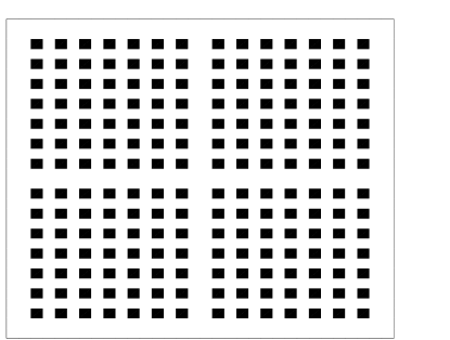
The composite is assumed to be built up according to Figure 1. The white part in the figure denotes a background material and the black parts an insulated material. The black squares are of size . We assume that the Lamé coefficients and take the values and on the insulated material, and and on the background material. In this experiment we have set and . Similarly, using subscript 1 for the insulated material and subscript 2 for the background material, we set and , for , where is the -dimensional identity matrix and . Furthermore, we have chosen to set (no external body forces) and .
The initial data must be zero on the boundary , so we have chosen to put and to the -projection of to . For the generalized finite element solution we have chosen and is given by (4.19).
The domain is discretized using a uniform triangulation. The reference solution is computed on a mesh of which resolves the fine parts (the black squares) in the material. The generalized finite element method (GFEM) in (4.16)-(4.18) is computed for five decreasing values of the mesh size, namely, with the patch sizes . For comparison, we also compute the corresponding classical finite element (FEM) solution on the coarse meshes using continuous piecewise affine polynomials for both spaces (P1-P1). The solutions satisfies (3.1)-(3.2) with replaced by and are denoted and respectively for . When computing these solutions we have evaluated the integrals exactly to avoid quadrature errors.
We have chosen to set and for all values of and for the reference solution. The solutions are compared at the time point .
Note that the implementation of the corrections in (4.18) given by
should not be computed explicitly at each time step. It is more efficient to compute , given by
where is the basis for . Now, since , we have the identity
With this approach, we only need to compute once before solving for the system (4.16)-(4.17) for .
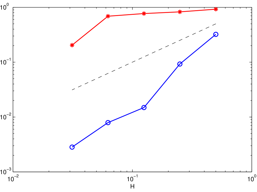
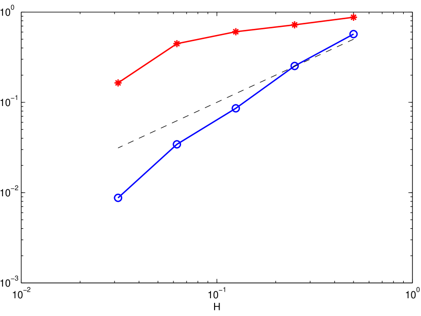
The relative errors in the -seminorm are shown in Figure 2. The left graph shows the relative errors for the displacement, and . The right graph shows the error for the temperature and . As expected the generalized finite element shows convergence of optimal order and outperforms the classical finite element.
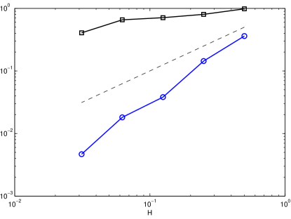
The second example shows the importance of the additional correction (4.18), which is designed to handle multiscale behavior in the coefficient . The computational domain, the spatial and the time discretization, and the patch sizes remain the same as in the first example. However, we let and in this case.
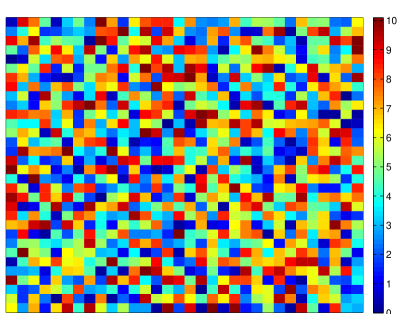
To test the influence of we let the other coefficients be constants, and , where the is the -dimensional identity matrix. The coefficient takes values between and according to Figure 3. The boxes are of size and, hence, the reference mesh of size is sufficiently small to resolve the variations in .
The initial data is set to and is the -projection of onto . For the generalized finite element solution we have chosen and is given by (4.19), as in our first example. Furthermore, we have chosen to set and .
The generalized finite element method (GFEM) in (4.16)-(4.18) is computed for the five decreasing values of the mesh size used in the first example. For comparison, we compute the generalized finite element without the additional correction on . In this case the system (4.16)-(4.18) simplifies to
The relative errors in the -seminorm are shown in Figure 2. The graph shows the errors for the displacement with correction for , and the error without correction for . As expected the GFEM with correction for shows convergence of optimal order and outperforms the GFEM without correction for . This is due to the fact that the constant in (4.13) (and hence also the constant in Theorem 5.2) depends on the variations in .
References
- [1] A. Abdulle and P. Henning. Localized orthogonal decomposition method for the wave equation with a continuum of scales. Submitted, 2014.
- [2] K.T. Andrews, P. Shi, M. Shillor, and S. Wright. Thermoelastic contact with Barber’s heat exchange condition. Appl. Math. Optim., 28(1):11–48, 1993.
- [3] I. Babuška and R. Lipton. Optimal local approximation spaces for generalized finite element methods with application to multiscale problems. Multiscale Model. Simul., 9(1):373–406, 2011.
- [4] I. Babuška and J. E. Osborn. Generalized finite element methods: their performance and their relation to mixed methods. SIAM J. Numer. Anal., 20(3):510–536, 1983.
- [5] M. A. Biot. General theory of three-dimensional consolidation. J. Appl. Phys., 18(2):155–164, 1941.
- [6] M. A. Biot. Thermoelasticity and irreversible thermodynamics. J. Appl. Phys., 27:240–253, 1956.
- [7] P.G. Ciarlet. Mathematical elasticity. Vol. I, volume 20 of Studies in Mathematics and its Applications. North-Holland Publishing Co., Amsterdam, 1988. Three-dimensional elasticity.
- [8] C. M. Dafermos. On the existence and the asymptotic stability of solutions to the equations of linear thermoelasticity. Arch. Rational Mech. Anal., 29:241–271, 1968.
- [9] Ch. Engwer, P. Henning, A. Målqvist, and D. Peterseim. Efficient implementation of the localized orthogonal decomposition method. Submitted.
- [10] A. Ern and S. Meunier. A posteriori error analysis of Euler-Galerkin approximations to coupled elliptic-parabolic problems. M2AN Math. Model. Numer. Anal., 43(2):353–375, 2009.
- [11] P. Henning and A. Målqvist. Localized orthogonal decomposition techniques for boundary value problems. SIAM J. Sci. Comput., 36(4):A1609–A1634, 2014.
- [12] P. Henning, A. Målqvist, and D. Peterseim. A localized orthogonal decomposition method for semi-linear elliptic problems. ESAIM Math. Model. Numer. Anal., 48(5):1331–1349, 2014.
- [13] P. Henning and A. Persson. A multiscale method for linear elasticity reducing poisson locking. Submitted.
- [14] T. J. R. Hughes, G. R. Feijóo, L. Mazzei, and J-B. Quincy. The variational multiscale method—a paradigm for computational mechanics. Comput. Methods Appl. Mech. Engrg., 166(1-2):3–24, 1998.
- [15] M. G. Larson and A. Målqvist. Adaptive variational multiscale methods based on a posteriori error estimation: energy norm estimates for elliptic problems. Comput. Methods Appl. Mech. Engrg., 196(21-24):2313–2324, 2007.
- [16] A. Målqvist and A. Persson. Multiscale techniques for parabolic equations. Submitted.
- [17] A. Målqvist and D. Peterseim. Localization of elliptic multiscale problems. Math. Comp., 83(290):2583–2603, 2014.
- [18] A. Målqvist and D. Peterseim. Computation of eigenvalues by numerical upscaling. Numer. Math., 130(2):337–361, 2015.
- [19] D. Peterseim. Variational multiscale stabilization and the exponential decay of fine-scale correctors. Submitted.
- [20] P. J. Phillips and M. F. Wheeler. A coupling of mixed and discontinuous galerkin finite-element methods for poroelasticity. Computational Geosciences, 12(4):417–435, 12 2008.
- [21] P. Shi and M. Shillor. Existence of a solution to the -dimensional problem of thermoelastic contact. Comm. Partial Differential Equations, 17(9-10):1597–1618, 1992.
- [22] R. E. Showalter. Diffusion in poro-elastic media. J. Math. Anal. Appl., 251(1):310–340, 2000.
- [23] X. Xu. The -dimensional quasistatic problem of thermoelastic contact with Barber’s heat exchange conditions. Adv. Math. Sci. Appl., 6(2):559–587, 1996.
- [24] A. Ženíšek. The existence and uniqueness theorem in Biot’s consolidation theory. Apl. Mat., 29(3):194–211, 1984.
- [25] A. Ženíšek. Finite element methods for coupled thermoelasticity and coupled consolidation of clay. RAIRO Anal. Numér., 18(2):183–205, 1984.