Influence of the energy-band structure on ultracold reactive processes in lattices

Abstract

We study theoretically ultracold collisions in quasi one-dimensional optical traps for bosonic and fermionic reactive molecules in the presence of a periodic potential along the trap axis. Elastic, reactive, and umklapp processes due to non-conservation of the center of mass motion are investigated for parameters of relevant experimental interest. The model naturally keeps into account the effect of excited energy bands and is particularly suited for being adapted to rigorous close-coupled calculations. Our formalism shows that a correct derivation of the parameters in tight-binding effective models must include the strong momentum dependence of the coupling constant we predict even for deep lattices.

I Introduction

Ultracold gases confined in optical lattices represent an extremely active area of theoretical and experimental research for quantum few and many-body physics Bloch (2005); Bloch et al. (2008). The flexibility in the choice of the lattice parameters and the variety of trappable atomic and molecular species allow the properties of these systems to be controlled with unprecedented accuracy. A variety of phases has been predicted and several have been observed in celebrated experiments on atomic quantum gases trapped in lattices of various dimensionality and structure Greiner et al. (2002); Paredes et al. (2004); Hadzibabic et al. (2006). Over the last decade, different dynamical aspects such as transport, few-body correlations, and the occurrence of geometric resonances have been studied experimentally under lattice confinement Ott et al. (2004); Tolra et al. (2004); Moritz et al. (2005); Fertig et al. (2005); Haller et al. (2010). It is now also possible to prepare cold or even Bose-condensed gases in excited bands of optical potentials Wirth et al. (2011).

Understanding the microscopic few-body collisional interaction is essential to model the macroscopic behavior of a gaz held in a lattice. Several papers focused on the two-atom problem in conditions where an harmonic confining potential restricts the motion to one or two dimensions Olshanii (1998); Petrov et al. (2000); Bolda et al. (2002); Micheli et al. (2010); Sala et al. (2012). The recent production of ultracold molecular samples has opened the way to the study of reactive processes at extremely low temperatures both in free space and in confined geometries. The combined effect of confinement and of a polarizing electric field has been studied both theoretically and experimentally in de Miranda et al. (2011), where the authors demonstrate that repulsion between polarized molecules held in a quasi-2D pancake geometry strongly suppresses the reaction probability and stabilizes the gaz. A theoretical analysis of reactions has also been carried out in quasi-1D optical tubes Simoni et al. (2015). In all these studies hopping between lattice sites is not included and the potential in the effectively free dimensions remains flat.

The periodic nature of the trapping optical lattice has been taken explicitly into account within tight binding lattice models Fedichev et al. (2004); Nygaard et al. (2008) and using a more general formalism Wouters and Orso (2006); Büchler (2010). Little is known about reaction dynamics in a periodic potential. Experimental work carried out at JILA on reactive polar molecules addresses the effect of a weak lattice (a corrugation) superimposed along the axis of an array of tubes Chotia et al. (2012). The authors speculate on the origin of the observed reaction rates and show that one can interpret the observed suppression of such inelastic processes as a manifestation of the quantum Zeno effect Zhu et al. (2014).

Main goal of the present paper is to model the two-body reaction dynamics in 1D geometries similar to the aforementioned experiment Chotia et al. (2012) using a more direct collisional approach. We solve an effective model where the short range reaction dynamics is represented by a completely adsorbing boundary condition. The key novelty of our formalism is the definition of a set of reference wavefunctions that include in a rigorous way the effect of the excited energy bands. While the formalism is applied to a simple yet realistic purely 1D model with a point-like interaction, it can in principle be readily incorporated in a full 3D close-coupled calculation such as the one of Ref. Simoni et al. (2015).

The paper is organized as follows. Sec. II describes the model, defines the scattering observables in terms of two-body Bloch functions, and introduces our numerical approach. Sec. III presents results for lattices of different strength for reactive molecules of both bosonic and fermionic nature. Approximations are developed and discussed. A short conclusion summarizes and puts into perspective the present work.

II Theoretical model

We consider ultracold molecules in a strongly confining harmonic potential along radial directions $x$ and $y$ in the presence of a weaker periodic sinusoidal optical potential along the axial direction $z$. The harmonic trapping frequency $\omega_{\perp}$ is the same for both radial directions. In the absence of the optical lattice, if the interaction potential is sufficiently short ranged one can describe the system as quasi-one-dimensional along the longitudinal $z$ axis. The practical criterion for van der Waals interactions with dispersion coefficient $C_{6}$ and particles of mass $m$ and reduced mass $\mu=m/2$ is that the van der Waals length ${\bar{a}}=0.5(2\mu C_{6}/\hbar^{2})^{1/4}$ be much smaller than the transverse oscillator length $a_{\perp}=\sqrt{\hbar/\mu\omega_{\perp}}$.

The K-Rb fermionic molecules studied at JILA have been found experimentally to be highly reactive Ospelkaus et al. (2010). In order to address this experimentally relevant case, this work will focus on universal reactive processes, in which all particle flux reaching a suitable short range region gives rise to reaction with unit probability Micheli et al. (2010). The typical size of this region can be taken to be on the order of $\sim 40a_{0}$, such that the potential beyond this boundary is well approximated by an isotropic van der Waals potential. Under such conditions the short-range collision dynamics for bosonic particles can be summarized by a pseudopotential $U_{a}=g\delta(z_{2}-z_{1})$ with complex coupling constant. The coupling constant can in turn be simply expressed in terms of the geometric parameters of the trap and of the van der Waals length as $g=2\hbar\omega_{\perp}{\bar{a}}(1-i)$ Micheli et al. (2010).

It is important for the following to stress that the pseudopotential conserves real CM momentum (as opposed to the quasimomentum) of the system. Also note that the pseudopotential cannot be directly used to model Fermions since due to Pauli exclusion principle the wavefunction strictly vanishes at zero interparticle separation. However, as it will be detailed in Sec. III D one can take advantage of a boson-fermion mapping procedure in order to apply with little modification the current formalism to fermionic particles as well.

Finally, the optical lattice along the longitudinal direction is taken of the form $U_{\rm L}(z)=u\sin^{2}(kz)=u\left[1-\cos({k_{\rm L}z})\right]/2$, where $u$ is the lattice depth, $k$ the laser wavevector, $k_{\rm L}\equiv 2k$ the lattice wavevector, related to the lattice period $a=2\pi/k_{\rm L}$. We assume that this lattice does not modify the effective 1D interatomic potential. This is only justified when the harmonic oscillator frequency $\omega_{\rm L}=k_{\rm L}\sqrt{u/2m}$, obtained by Taylor expanding $U_{\rm L}$ near a minimum of the lattice potential, is much smaller than $\omega_{\perp}$. The lattice depth will henceforth be expressed in terms of the lattice recoil energy for one molecule defined as $E_{\rm R}=\hbar^{2}k_{\rm L}^{2}/(2m)$. Note this quantity is four times larger than the laser recoil energy $\hbar^{2}k^{2}/(2m)$ which is often used in experimental work.

II.1 Band structure and free Bloch waves

In the absence of the effective interatomic potential the wavefunction of a pair of molecules is described by a product of 1D Bloch waves $|\phi_{p_{1}}^{m}\rangle\otimes|\phi_{p_{2}}^{n}\rangle$, labeled by quasi-momenta $p_{\alpha}$ for particle $\alpha$ in energy zones $m$ and $n$, respectively. The energy of a single-particle Bloch state $|\phi_{p}^{m}\rangle$ is ${\cal E}_{m}(p)$ and the single-atom states are quasi-momentum normalized $\langle\phi_{p^{\prime}}^{m}|\phi_{p}^{n}\rangle=\delta(p^{\prime}-p)\delta_{mn}$. For describing the effects of the interaction it is convenient to introduce the relative and CM quasi-momenta $\{q=(p_{1}-p_{2})/2,Q=p_{1}+p_{2}\}$ and the two-particle state $|\Phi_{qQ}^{mn}\rangle=|v_{mn}(q,Q)|^{-1/2}\left(|\phi_{Q/2+q}^{m}\rangle\otimes|\phi_{Q/2-q}^{n}\rangle\right)$. Such state has energy $E_{mn}(q,Q)={\cal E}_{m}(Q/2+q)+{\cal E}_{n}(Q/2-q)$ and $v_{mn}(q,Q)={\partial E_{mn}}/{\partial(\hbar q)}$ is the relative group velocity for particles in zones $m$ and $n$. In this way pair states are quasi-momentum normalized for the CM quasi-momentum and energy or flux normalized for the relative quasi-momentum, i.e. $\langle\Phi_{q^{\prime}Q^{\prime}}^{m^{\prime}n^{\prime}}|\Phi_{qQ}^{mn}\rangle=\delta\left[E_{mn}(q^{\prime},Q^{\prime})-E_{mn}(q,Q)\right]\delta(Q^{\prime}-Q)\delta_{mm^{\prime}}\delta_{nn^{\prime}}$. For notational simplicity, when possible we will henceforth condense the double zone index into a single Greek letter $\alpha\equiv(m,n)$.

When two molecules collide with relative quasi-momentum $q$ and CM quasi-momentum $Q$ the interatomic potential can induce coupling to different states $\Phi_{q^{\prime}Q^{\prime}}$ such that total energy is conserved $E^{\prime}=E$ and the CM quasimomentum varies by a multiple of a lattice vector $Q^{\prime}=Q\pmod{k_{\rm L}}$. Such processes are known as umklapp collisions in solid state physics (see e.g. Ref Ashcroft and Mermin (1976)) and have been experimentally observed in Campbell et al. (2006) where they were described in terms of a phase matching condition. In a quasi-1D lattice such condition of energy and momentum conservation is restrictive and only a small number of allowed states exist for given $E$ and $Q$. Umklapp processes are more conveniently discussed by choosing the fundamental reciprocal lattice cell $\{q,Q\}\in[-k_{\rm L}/2,k_{\rm L}/2]\times[0,k_{\rm L}]$ where $Q$ is unambiguously defined. Thus, when restricted to this specific unit cell umklapp collisions strictly, not only $\pmod{k_{\rm L}}$, do conserve $Q$.

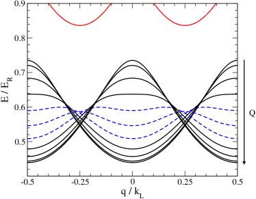
Figure 1: Two-particle energy as a function of $q$ in an optical lattice of depth $u=0.5~{}E_{\rm R}$ for discrete values of total quasimomentum $Q$ varying from $0$ to $k_{\rm L}$ in step of $0.1~{}k_{\rm L}$ in the sense of the arrow. Both molecules are in the fundamental band. The dashed curves correspond to CM quasimomenta for which umklapp collisions are allowed (see text). The lower limit of the first excited energy band is visible in the upper part of the panel.

Fig. (1) shows the relative-motion energy dispersion relation of two molecules in the fundamental band for selected values of $Q$. It is easy to show that square lattice periodicity implies that the reciprocal lattice points $(q,Q)$ and $(q-k_{\rm L},Q)$ only differ by a reciprocal lattice vectors. The energy is thus periodic in $q$ at the cell edges, i.e. $E_{mm}(-k_{\rm L}/2,Q)=E_{mm}(k_{\rm L}/2,Q)$ for particles in the same band. If particles belong to different energy bands the former symmetry relation reads $E_{mn}(-k_{\rm L}/2,Q)=E_{nm}(k_{\rm L}/2,Q)$.

We consider in this work identical particle scattering and by the symmetrization principle the range of $q$ can be restricted to half space only ($q\geq 0$) if particles are in the same energy band. For particles in different bands, one has to consider either $q\geq 0$ and both $(m,n)$ and $(n,m)$ combinations, or both positive and negative values of $q$ with the restriction $m>n$. With this proviso, if for a given $Q$ and energy $E$ of the incoming molecules the dispersion relation $E_{mn}(q,Q)$ presents at least a maximum or minimum in $q$, umklapp collisions in the given band will occur at energies $E$ such that the equation $E(q,Q)=E$ admits a double solution (with the restriction $q>0$ if $m=n$). Sample values of $Q$ for which this condition is verified are shown by dashed curves in the figure. On the converse, if the dispersion relation is monotonic no umklapp processes will be possible. Note that if the lattice is weak or collisions take place in excited bands the energy gap will become sufficiently small that umklapp processes can take place not only intra-, as in the case of Fig. (1), but also inter-band.

If the lattice is strong enough the dispersion relation is explicitly known in the tight binding approximation. For one molecule in energy band $n$ it can be written as ${\cal E}_{m}(p_{1})=D_{m}-J_{m}\cos(ap_{1})]$ Ashcroft and Mermin (1976) where $|J_{m}|$ is the energy half-bandwidth and the constant $D_{m}$ in the harmonic approximation is related to the harmonic frequency at the bottom of the well as $D_{m}=\hbar\omega_{\rm L}(m+1/2)$. Since potential is separable, energy is additive $E_{mn}={\cal E}_{m}(p_{1})+{\cal E}_{n}(p_{2})$ and simple algebra gives

$$E_{mn}(q,Q) = D_{m}+D_{n}+(J_{m}-J_{n})\sin(aQ/2)\sin(aq)$$ (1)

$$- (J_{m}+J_{n})\cos(aQ/2)\cos(aq).$$

It is easy so show that $E_{mn}(q,Q)$ is monotonic in the interval $q\in[0,k_{\rm L}/2]$ for any $Q$ if $n=m$, otherwise it admits therein a single maximum or minimum for $Q\neq 0$. The umklapp collisions will therefore occur in the tight binding limit if and only if the colliding particles belong to different single-particle energy bands.

II.2 Scattering wavefunction and scattering observables

The incoming wavefunction for the collision will be taken as a Bloch wave $\Phi_{q,Q}^{\alpha}(z,Z)$ with relative group velocity $v<0$, i.e. moving opposite to the $z$ direction. Outside the range of the interatomic potential ($z\to\infty$) the wave function is written as the sum of an incoming plus outgoing scattered Bloch waves

$$\Psi_{qQ}^{\alpha}=\Phi_{qQ}^{\alpha}\pm\sum_{q^{\prime}Q^{\prime}\alpha^{\prime}}\Phi^{\alpha^{\prime}}_{q^{\prime}Q^{\prime}}S(q^{\prime}Q^{\prime}\alpha^{\prime}\leftarrow qQ\alpha)$$ (2)

where the upper (lower) sign holds for bosons (fermions). The sum includes all purely real relative quasi-momenta $q^{\prime}$ such that $E_{\alpha^{\prime}}(q^{\prime},Q^{\prime})=E_{\alpha}(q,Q)$ in zone $\alpha^{\prime}$ for $Q^{\prime}=Q\pmod{k_{\rm L}}$. Since we are imposing outgoing boundary conditions, the scattered waves on the right hand side must be chosen with relative group velocity in the direction of the positive $z$ axis for $z>0$.

The sum also contains functions that decrease exponentially with increasing $z$ characterized by complex relative quasi-momentum with $\Im q>0$. In the language of scattering theory, we will often term the propagating (evanescent) waves with $\Im q=0$ ( $\Im q\neq 0$) the open (closed) channels of the collision. An algebraic procedure to determine both kind of Bloch waves will be the subject of Sec. III C.

For a real non-absorbing potential, the choice of flux normalized reference functions and conservation of probability result in unitarity of the $S$ matrix block formed by all the $S(q^{\prime}Q^{\prime}\alpha^{\prime}\leftarrow qQ\alpha)$ elements with purely real $q$ and $q^{\prime}$. This is not any longer true for our potential that aims at modelling reactive processes through the introduction of a nonzero imaginary part. It is indeed the difference to unitarity that gives the reaction probability; See Eq. (4) below.

The scattering matrix encompasses all information about the scattering process. Our conventions on the propagation directions of the incoming and scattered waves allow the same expressions for the scattering observables to be used as in the no-lattice case Simoni et al. (2015). Thus, the elastic scattering rate is expressed in terms of the scattering matrix as

$${\cal K}^{\rm el}_{\alpha}(q,Q)=|v_{\alpha}(q,Q)|\left|1-S(qQ\alpha\leftarrow qQ\alpha)\right|^{2}$$ (3)

Another quantity of experimental interest is the reaction probability

$$P^{\rm r}_{\alpha}(q,Q)=1-\sum_{q^{\prime}Q^{\prime}\alpha^{\prime}}|S(q^{\prime}Q^{\prime}\alpha^{\prime}\leftarrow qQ\alpha)|^{2}$$ (4)

which in the formalism stems from the lack of unitarity of the $S$-matrix due to the complex nature of the coupling constant. The summed probability for umklapp processes, that can be interpreted as superelastic collisions taking place at fixed total energy, is given by

$$P^{\rm u}_{\alpha}(q,Q)=\sideset{}{{}^{\prime}}{\sum}_{q^{\prime}Q^{\prime}\alpha^{\prime}}|S(q^{\prime}Q^{\prime}\alpha^{\prime}\leftarrow qQ\alpha)|^{2}$$ (5)

where the sum $\sum^{\prime}$ is restricted to $\{q^{\prime}Q^{\prime}\alpha^{\prime}\}\neq\{qQ\alpha\}$. Such scattering quantities are in principle measurable in a reference frame in uniform motion with velocity equal to the CM group velocity $v_{\rm CM}={\partial E}/{\partial(\hbar Q)}$ of the colliding particles.

The effect of the lattice can be summarized in quasimomentum-dependent scattering lengths defined for bosons and fermions respectively as

$$a^{\rm B}_{\alpha}(q,Q)=\frac{\hbar}{\mu|v_{\alpha}(q,Q)|k_{\alpha}(q,Q)}$$ (6)

and

$$a^{\rm F}_{\alpha}(q,Q)=-\frac{\hbar\,k_{\alpha}(q,Q)}{\mu|v_{\alpha}(q,Q)|}$$ (7)

where $\mu=m/2$ is the reduced mass and $k_{\alpha}(q,Q)\equiv i\left[1-S(qQ\alpha\leftarrow qQ\alpha)\right]/\left[1+S(qQ\alpha\leftarrow qQ\alpha)\right]$. If one writes as usual $S=e^{2i\delta}$, the quantity $k$ is seen to simply represents the tangent of the (generally complex) phase shift $\delta$. Note that the $a^{\rm F,B}$ above reduce to the standard ones in free space in the absence of the lattice. Finally, boson scattering can also be conveniently described by introducing an effective momentum-dependent coupling constant in band $\alpha$

$$g^{\rm eff}_{\alpha}(q,Q)=-\frac{\hbar^{2}}{\mu\,a^{\rm B}_{\alpha}(q,Q)}.$$ (8)

This quantity is the effective interaction that after averaging over a period of the center-of-mass coordinate gives a scattering matrix element in the elastic channel equal to the actual one. The imaginary part of $g_{\rm eff}$ accounts for the combined effect of reactive and umklapp processes. In the absence of optical lattice $g^{\rm eff}(q,Q)$ reduces to $g$ as expected.

II.3 Determining the reference functions

For notational convenience in next two sections we adopt as the units of momentum, length, and energy the lattice vector $k_{\rm L}$, its inverse $k_{\rm L}^{-1}$ and the lattice recoil energy $E_{\rm R}$, respectively. The coupling constant will thus be expressed in units $E_{\rm R}/k_{\rm L}$.

The reference functions used in Eq. (2) can be built as follows. According to the Bloch theorem, even in the presence of the interaction the scattering wavefunction transforms as a Bloch function $\Psi_{qQ}(z,Z+2\pi)=e^{i2\pi Q}\Psi_{q,Q}(z,Z)$ under CM coordinate translations of period $2\pi$. Bloch’s theorem allows then $\Psi$ to be expressed in the general form $\Psi_{qQ}(z,Z)=e^{iQZ}\sum_{n}e^{inZ}\psi_{qQ,n}(z)$.

In order to represent the interacting $\Psi$, non interacting reference functions must therefore be built with the given (real) value of $Q$. To this aim, Bloch theorem now applied to both the CM and relative coordinates implies that the pair wavefunction in the absence of the interaction can be written in the form $\Phi_{q,Q}(z,Z)=e^{i(QZ+qz)}u_{qQ}(z,Z)$ with $u_{qQ}$ periodic with the lattice periodicity. Similarly, it can be easily verified by direct differentiation that any spatial derivative of $\Phi_{qQ}$ can be expressed in Bloch’s form as well. In particular, $\chi_{qQ}(z,Z)\equiv\partial_{z}\Phi_{qQ}(z,Z)=e^{i(QZ+qz)}v_{qQ}(z,Z)$ with $v_{qQ}=iqu_{qQ}+\partial_{z}u_{qQ}$ a function periodic on the lattice.

With these definitions, the second order time independent Schrödinger equation can be rewritten as a set of two coupled partial differential equations of order one

$$i\frac{\partial}{\partial z}u_{qQ}-iv_{qQ}=qu_{qQ}$$

$$i\frac{\partial}{\partial z}v_{qQ}+\dfrac{i}{2}\left[E-\frac{1}{2}(-i\frac{\partial}{\partial Z}+Q)^{2}-V_{\rm L}(z,Z)\right]u_{qQ}=qv_{qQ}$$

in the form of an eigenvalue problem for the unknown spatial functions $u_{qQ}$ and $v_{qQ}$ and the eigenvalue $q$. The operator on the lhs can be considered a matrix differential operator acting on column vector wavefunctions ${\vec{w}}_{qQ}\equiv(u_{qQ},v_{qQ})^{t}$ in a lattice unit cell. One can verify that such operator is hermitian with respect to the symplectic inner product $\langle{\vec{w}}_{q^{\prime}Q}|{\vec{w}}_{qQ}\rangle_{s}\equiv\langle u_{q^{\prime}Q}|v_{qQ}\rangle-\langle v_{q^{\prime}Q}|u_{qQ}\rangle$, where the scalar product on the rhs is the standard one over a unit cell. Since the symplectic inner product is not positive-definite it is not possible to show that $q$ is real in general. One can however deduce following the standard proof that if $q^{\prime}\neq q^{*}$ then the symplectic orthogonality condition $\langle{\vec{w}}_{q^{\prime}Q}|{\vec{w}}_{qQ}\rangle_{s}\propto\delta_{q^{\prime}q^{*}}$ holds.

Additional properties follow from the lattice symmetries. First, since the lattice potential $V_{\rm L}$ is real, taking the conjugate of (II.3) shows that if ${\vec{w}}_{qQ}$ is eigenfunction with eigenvalue $q$ then ${\vec{w}}_{qQ}^{*}={\vec{w}}_{-q^{*}-Q}$ is eigenfunction of the corresponding problem with quasimomentum $-Q$ and eigenvalue $q^{*}$ (time-reversal property). Moreover, the particles being identical, irrespective of the nature of $V_{\rm L}$ one has $V_{\rm L}(-z,Z)=V_{\rm L}(z,Z)$. Application of the permutation operation $z\to-z$ to (II.3) shows that if $q$ is eigenvalue with eigenfunction $(u_{qQ},v_{qQ})$ then $-q$ is also eigenvalue with eigenvector $(u_{-qQ}(z,Z),v_{-qQ}(z,Z))=(u_{qQ}(-z,Z),-v_{qQ}(-z,Z))$. Finally, reflection of both coordinates $(z,Z)\to(-z,-Z)$ about the center of symmetry of the lattice also leaves $V_{\rm L}$ invariant. One concludes that if $(u_{qQ},v_{qQ})$ solves Eq. (II.3) with eigenvalue $q$, $(u_{-q-Q}(z,Z),v_{-q-Q}(z,Z))=(u_{qQ}(-z,-Z),-v_{qQ}(-z,-Z))$ will also be solution of the equation with eigenvalue $-q$ and CM quasimomentum $Q$. Note that if $q$ is purely real or purely imaginary, only two of the four solutions with quasimomenta $\pm q$ and $\pm q^{*}$ generated by the symmetry operations above will be linearly independent.

Equations (II.3) can be solved algebraically noting that the periodic nature of the functions $u_{qQ}$ and $v_{qQ}$ allows the latter to be developed in a 2D Fourier series

$$u_{qQ}(z,Z)=\sum_{\vec{K}}a_{\vec{K}}(q,Q)e^{i{\vec{K}}\cdot{\vec{r}}}$$ (10)

and

$$v_{qQ}(z,Z)=\sum_{\vec{K}}b_{\vec{K}}(q,Q)e^{i{\vec{K}}\cdot{\vec{r}}},$$ (11)

where the sum is over all reciprocal lattice vectors $\vec{K}$, and using standard numerical eigenvalue solvers. The resulting families of discrete eigenvalues $q$ depend on the two real parameter $Q$ and $E$. Since the bidimensional quasimomentum vector of components $(q,Q)$ is defined $\pmod{\vec{K}}$, as in the discussion of umklapp processes it is convenient to choose the specific unit cell $(\Re q,Q)\in[-1/2,1/2]\times[0,1]$. Note that the imaginary part $\Im q$ is to be left unrestricted since Bragg periodicity only concerns the real part of the quasimomentum.

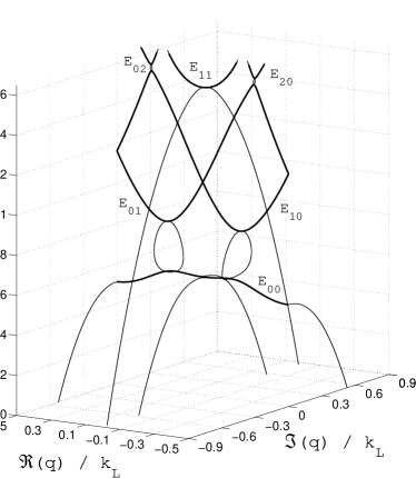
Figure 2: Evolution with $E$ of the complex relative quasimomentum determined from the solution of Eq. (II.3) for $Q=0.6~{}k_{\rm L}$ and $u=0.5~{}E_{\rm R}$. Propagating Bloch waves are characterized by a purely real $q$ (heavy lines) describing energy bands $E_{mn}$. Thin lines represent the quasimomenta of evanescent waves with $\Im q\neq 0$ (see text). Two additional curves with larger $|\Im q|$ and $\Re q=0$ fall in the range of the figure but have not been drawn to improve plot readability.

It is instructive to study the evolution of eigenvalues $q$ with total energy at fixed values of total quasimomentum; See Fig. (3) for the selected case $Q=0.6$. With reference to the figure, in the allowed energy regions the energy band structure highlighted by thick lines is retrieved as expected. One can recognize in particular the fundamental band dispersion $E_{00}$ with two extrema already depicted in Fig. (1) and the first excited band structure formed by the $E_{01}$ and $E_{10}$ components. The symmetry $E_{01}(q,Q)=E_{10}(-q,Q)$ is apparent. The bottoms of higher energy bands $E_{11}$, $E_{20}$ and $E_{02}$ are also visible.

If $E$ is below the lowest limit of the fundamental band all $q$ have nonvanishing imaginary part and no propagating waves exist. In Fig. (3) one identifies four branches located in the $\Re q=0$ plane and two in the $\Re q=\pm 1/2$ planes, respectively. That is, below the minimum of $E_{00}$ one finds six intersections between any horizontal plane and the curves of complex $q$ depicted in the plot.

These curves correspond to evanescent-character waves and merge at critical points with the dispersion curves of the authorized energy zones. In fact, $|\Im q|$ decreases with increasing $E$, and as $|\Im q|\to 0$ two branches merge with $E_{00}$ at the edge of the Brillouin zone $\Re q=\pm k_{\rm L}/2$ where they become of propagating character. At slightly larger energy two branches with purely imaginary argument $q$ merge with the curve $E_{00}$ at the relative minimum of the latter. The two remaining curves with $\Re q=0$ in the figure merge at the bottom of $E_{11}$ at still larger energies ($E\simeq 1.5$).

The behavior near the upper limit of $E_{00}$ is particularly interesting. As the value of energy varies from below to above the upper band limit two new branches with $\Im q\neq 0$ appear above each maximum. These curves are non planar and join again near the minima at the bottom of the $E_{10}$ and $E_{01}$ bands. The existence of these “smoke rings” connecting band edges is necessary since quantum states cannot disappear as the parameter $E$ is made to vary. Similar ring structures connecting the top of $E_{10}$ and $E_{01}$ with the bottom of $E_{20}$ and $E_{02}$ are also (barely) visible in the figure.

II.4 Scattering matrix calculation

Next we note that $2\pi$-periodicity in the $Z$ coordinate alone allows one to write $\Phi_{qQ}(z,Z)=e^{iQZ}\sum_{n}e^{inZ}\eta_{qQ,n}(z)$ and $\chi_{qQ}(z,Z)=e^{iQZ}\sum_{n}e^{inZ}\xi_{qQ,n}(z)$, where

$$\eta_{qQ,n}(z) = \frac{e^{iqz}}{2\pi}\int_{0}^{2\pi}dZe^{-inZ}u_{qQ}(z,Z)$$

$$\xi_{qQ,n}(z) = \frac{e^{iqz}}{2\pi}\int_{0}^{2\pi}dZe^{-inZ}v_{qQ}(z,Z).$$ (12)

For a given truncation order of the Fourier series in $Z$ it is possible to arrange the coefficients $\eta_{qQ,n}$ and $\xi_{qQ,n}$ into finite square solution matrices ${\boldsymbol{\eta}}_{\pm}$ and ${\boldsymbol{\xi}}_{\pm}$, where ${\boldsymbol{\eta}}_{-}$ (resp. ${\boldsymbol{\eta}}_{+}$) contains along the columns propagating Bloch waves with $v<0$ ($v>0$) and evanescent Bloch waves exponentially decreasing towards $z>0$ ($z<0$).

Combining the symmetry properties stated below Eq. (II.3) one can easily prove the symmetry relation $\eta_{qQ,n}^{*}(z)=\eta_{-q^{*}Q,n}(z)$ and $\xi_{qQ,n}^{*}(z)=\xi_{-q^{*}Q,n}(z)$. As already remarked, four independent degenerate solutions may exist with momenta $\pm q$ and $\pm q^{*}$. In this case, which only may occur for closed channels, we find it convenient to form real reference functions according to $(\eta_{\pm qQ,n}+\eta_{\mp q^{*}Q,n})$ and $-i(\eta_{\pm qQ,n}-\eta_{\mp q^{*}Q,n})$. Analogous definitions are used to construct the derivatives $\xi$.

With these conventions the matrix form of Eq. (2) is

$${\boldsymbol{\psi}}(z)={\boldsymbol{\eta}}_{-}(z)+{\boldsymbol{\eta}}_{+}(z){\mathbf{S}}$$ (13)

where $\boldsymbol{\psi}$ has elements $\psi_{qQ,n}$, while the $z$ derivative is expressed as

$$\frac{\partial}{\partial z}{\boldsymbol{\psi}}(z)={\boldsymbol{\xi}}_{-}(z)+{\boldsymbol{\xi}}_{+}(z){\mathbf{S}}.$$ (14)

In order to determine the scattering matrix we note that our zero-range model interaction conserves real (as opposed to quasi) total momentum and imposes a discontinuity to the relative coordinate derivative at the origin

$$\left.\frac{\partial}{\partial z}\psi_{qQ,n}\right|_{0^{+}}-\left.\frac{\partial}{\partial z}\psi_{qQ,n}\right|_{0^{-}}=2\left.\frac{\partial}{\partial z}\psi_{qQ,n}\right|_{0^{+}}=\frac{g}{2}\psi_{qQ,n}(0)$$ (15)

where the first equality follows from the even character of the bosonic wavefunction. This set of conditions can be summarized in the logarithmic derivative of the matrix solution evaluated at the origin ${\mathbf{Z}}\equiv(\partial_{z}{\boldsymbol{\psi}}){\boldsymbol{\psi}}^{-1}=(g/4){\mathbf{1}}$. Finally, imposing the asymptotic form (13) and following the standard matching procedure Simoni and Launay (2011) the scattering matrix can be determined in terms of $\mathbf{Z}$ by solving the linear system

$$\left[{\boldsymbol{\xi}}_{+}(0^{+})-{\mathbf{Z}}{\boldsymbol{\eta}}_{+}(0\right]{\mathbf{S}}=\left[{\mathbf{Z}}{\boldsymbol{\eta}}_{-}(0)-{\boldsymbol{\xi}}_{-}(0^{+})\right].$$ (16)

For fermions the condition dictated by the zero-range potential is of no practical use since it is identically verified by any wavefunction asymmetric in $z$. Use of more sophisticate pseudopotentials valid for fermions can be avoided by the simpler prescription of Ref. Granger and Blume (2004). In this approach, resulting from a mapping between bosons and fermions valid in dimension one, the fermionic problem is solved as if the particles were bosons with a mapped coupling constant

$$\frac{g_{\rm map}}{a_{\perp}\hbar\omega_{\perp}}=-\frac{a_{\perp}}{a^{\rm F}_{0}}.$$ (17)

Here the $a^{\rm F}_{0}$ is the 1D scattering length for fermions in the absence of the optical lattice, which can be determined analytically for universal scattering in tubes Micheli et al. (2010). Substituting the latter equation into (17) one obtains

$$\frac{g_{\rm map}}{a_{\perp}\hbar\omega_{\perp}}=\frac{a_{\perp}^{3}}{12{\bar{a}}^{2}{\bar{a}}_{1}}(1-i),$$ (18)

where ${\bar{a}}_{1}=1.064~{}\bar{a}$. Note that fermions, which due to Pauli principle are weakly interacting, are mapped to a bosonic problem implying strong interactions, i.e. the $g_{\rm map}$ constant above is large in natural units. The scattering matrix ${\mathbf{S}}_{\rm map}$ is computed with the mapped interaction exactly as for bosons and as a final step simply transformed to the physical fermionic counterpart ${\mathbf{S}}^{\rm F}=-{\mathbf{S}}_{\rm map}$.

II.5 Wigner threshold laws

In the presence of a lattice Wigner threshold laws describe elastic and inelastic processes when the initial or final state relative group velocity approaches zero. This naturally generalizes the notion of Wigner laws for free scattering, which is expressed in terms of momenta or equivalently in terms of velocities. In a periodic lattice however, unlike in free space, a zero group velocity does not only occur for $q\to 0$; see Fig. (3) for the fundamental band case. Threshold laws will therefore also apply at locations in the Brillouin zone where the group velocities of the two molecules are close, under the condition that they must be expressed in terms of $v$ rather than $q$. In fact, the Wigner laws essentially arise from the density of energy states for the relative motion $\rho_{\epsilon}$, and in a lattice $\rho_{\epsilon}\propto(\partial E/\partial q)^{-1}=v^{-1}$.

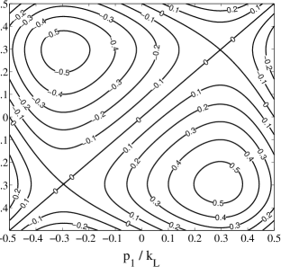
Figure 3: The relative group velocity $v$ of two particles in the first energy band for a lattice depth $u=E_{\rm R}$. Beyond being obviously zero for $p_{1}=p_{2}$ the velocity $v$ also vanishes for $q>0$ along nontrivial curves where the single particle group velocities are equal.

With this proviso, threshold laws can be expressed on the same footing as e.g. in Ref. Simoni and Launay (2011) with the scaling behavior typical of dimension one. For bosons, the elastic collision rate ${\cal K}^{\rm el,B}\sim v$ and both the umklapp and the reactive probability vanish with the group velocity of the incoming particles as $P^{\rm r,u}\sim v$. Moreover, if the relative group velocity $v^{\prime}$ of the products of a superelastic umklapp collisions is small, the probability for the umklapp process behaves as $P^{\rm u}\sim v^{\prime}$. The $P^{\rm u}$ probability drops therefore continuously to zero as the exit channels for the superelastic process become energetically closed.

The Wigner laws valid for bosons also hold for identical particles of fermionic nature, with the exception of the elastic collision rate that vanishes for $q\to 0$ as ${\cal K}^{\rm el,F}\sim v^{3}$ for particles in the same energy band. Note that the reciprocal-space point of coordinates $(q=k_{\rm L}/2,Q)$ can be brought into $(q=0,Q+k_{\rm L})$ by a reciprocal lattice vector translation of $k_{\rm L}$ parallel to the $p_{2}$ axis. As a consequence, the Wigner laws for $q\to 0$ and $q\to\pm k_{\rm L}/2$ are the same.

Finally, the Wigner laws imply that for bosons the quantity $g^{\rm eff}$ is finite at the lower or upper limit of the energy band occurring at $q=0$. If the energy band limit occurs at nonzero values of $q$ the $g^{\rm eff}$ vanishes. Similarly, for fermionic molecules the momentum dependent scattering lengths $a^{\rm F}(q,Q)$ tends to a finite quantity if the band edge occurs at $q=0$ and vanishes otherwise.

Les us examine in more detail the threshold behavior of the bosonic scattering matrix elements. To this aim, we fix a specific value of $Q=0.4~{} k_{\rm L}$ such that energy band limits of different nature $E_{i}$ ($i=1,2,3$) exist in the dispersion relation; See upper panel of Fig. (4). If $E<E_{1}$ no open channels (propagating waves) exist. As energy increases above $E_{1}$ one symmetrized collision channel becomes available. As shown in the lower panel of Fig. (4) $E\to E_{1}^{+}$ the unique $S$-matrix element $S_{11}\to-1$. In terms of distinguishable particles this behavior would amount to reflection with unit probability.

At the second threshold $E_{2}$ an additional channel with $q=k_{\rm L}/2$ becomes energetically open. The matrix element $S_{11}$ is therein continuous with discontinuous derivative, the new elastic element $S_{22}\to-1$ as $E\to E_{2}^{+}$, whereas the transition amplitude $S_{12}$ vanishes at threshold. Finally, for $E\to E_{3}^{-}$ the two open channel states tend to coalesce and the $S$-matrix tends to a finite limit with elements $S_{11}=S_{22}=0$ and $S_{12}=-1$. This result is somehow expected, since exactly at threshold $E_{3}$ there is only one quantum state and the rates for elastic and umklapp scattering must therefore become equal there.

The fermionic scattering matrix elements simply behave as $S^{\rm F}=-S^{\rm B}$.

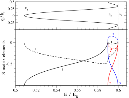
Figure 4: Upper panel : energy dispersion relation for two particles in a lattice of depth $u=0.5~{} E_{\rm R}$ and $Q=0.4~{} k_{\rm L}$. Dotted lines denote energy thresholds for collision channels (see text). Lower panel : real (full line) and imaginary part (dashed line) of scattering matrix elements. Labels $1,2$ and $3$ denote the elements $S_{11}$, $S_{22}$, and $S_{12}$ defined in the text, respectively.

II.6 One and two-channel models

Is is instructive to display at first the explicit structure of the scattering matrix within a minimal model with only open channels therefore neglecting the influence of the closed channels. Let us first consider the bosonic case. Calculation in the presence of multiple open channels is more easily performed using standing wave solutions defined as ${\boldsymbol{\eta}}_{1}=\left({\boldsymbol{\eta}}_{+}+{\boldsymbol{\eta}}_{-}\right)/2$ and ${\boldsymbol{\eta}}_{2}=-i\left({\boldsymbol{\eta}}_{+}-{\boldsymbol{\eta}}_{-}\right)/2$. Such asymptotic reference function are real by virtue of the symmetry property ${\boldsymbol{\eta}}_{-}^{*}={\boldsymbol{\eta}}_{+}$ below Eq. (II.3). Derivative matrices ${\boldsymbol{\xi}}_{1}$ and ${\boldsymbol{\xi}}_{2}$ are likewise represented in terms of ${\boldsymbol{\xi}}_{+}$ and ${\boldsymbol{\xi}}_{-}$.

By replacing standing waves for propagating waves, the asymptotic form (13) defines the reactance matrix $\mathbf{K}$. System of equations (16) becomes

$${\boldsymbol{\xi}}_{2}(0^{+}){\mathbf{K}}={\mathbf{Z}}{\boldsymbol{\eta}}_{1}(0).$$ (19)

Right multiplication of the system (19) by ${\boldsymbol{\eta}}_{1}^{t}(0)$ gives the solution ${\mathbf{K}}=({\boldsymbol{\eta}}_{1}^{t}{\boldsymbol{\xi}}_{2})^{-1}({\boldsymbol{\eta}}_{1}^{t}{\mathbf{Z}}{\boldsymbol{\eta}}_{1})$, where the $0^{+}$ argument has been omitted.

Observing that ${\boldsymbol{\eta}}_{2}(0)$ vanishes, the matrix ${\boldsymbol{\eta}}_{1}^{t}(0){\boldsymbol{\xi}}_{2}(0^{+})$ is identified as the value at the origin of the Wronskian

$$\mathbf{W}={\boldsymbol{\eta}}_{1}^{t}(z){\boldsymbol{\xi}}_{2}(z)-{\boldsymbol{\xi}}_{1}^{t}(z){\boldsymbol{\eta}}_{2}(z)$$ (20)

of linearly independent solution matrices of the Schrödinger equation for a given $Q$. Since the Wronskian is a constant matrix, integrating both sides of Eq. (20) with respect to $z$ and using Eq. (E.6) in the appendix of Ref. Ashcroft and Mermin (1976) to recover the group velocity as well as the symplectic orthogonality condition below Eq. (II.3) one obtains that ${\mathbf{W}}=a^{-1}{\mathbf{1}}$. Had we used momentum- rather than energy-normalized reference functions, the Wronskian would have been proportional to a diagonal matrix with entries the relative velocities. When applied to closed channels Eq. (E.6) defines a purely imaginary velocity that, while nonphysical, will play an important role in the following.

The scattering matrix is expressed in terms of $\mathbf{K}$ using the Cayley transform ${\mathbf{S}}=({\mathbf{1}}+i{\mathbf{K}})({\mathbf{1}}-i{\mathbf{K}})^{-1}$. The present approach is equivalent to the unitarized Born approximation, where the reactance matrix is computed in the first order Born approximation and the scattering matrix obtained through the Cayley transform is automatically unitary if interaction is real.

To be definite, let us consider the situation where two channels characterized by relative quasimomentum $q_{i}$ and corresponding velocity $v_{i}\equiv v_{\alpha}(q_{i},Q)$ ($i=1,2$) are energetically available in two-particle band $\alpha$ for total quasimomentum $Q$. Simple matrix algebra gives

$$S=\left(\begin{array}[]{cc}\dfrac{(g^{\alpha}_{12})^{2}-(g^{\alpha}_{11}+i\hbar v_{1})(g^{\alpha}_{22}-i\hbar v_{2})}{(g^{\alpha}_{11}-i\hbar v_{1})(g^{\alpha}_{22}-i\hbar v_{2})-(g^{\alpha}_{12})^{2}}&\dfrac{2i\hbar g^{\alpha}_{12}\sqrt{v_{1}v_{2}}}{(g^{\alpha}_{11}-i\hbar v_{1})(g^{\alpha}_{22}-i\hbar v_{2})-(g^{\alpha}_{12})^{2}}\\[8.61108pt] \dfrac{2i\hbar g^{\alpha}_{21}\sqrt{v_{1}v_{2}}}{(g^{\alpha}_{11}-i\hbar v_{1})(g^{\alpha}_{22}-i\hbar v_{2})-(g^{\alpha}_{12})^{2}}&\dfrac{(g^{\alpha}_{12})^{2}-(g^{\alpha}_{11}-i\hbar v_{1})(g^{\alpha}_{22}+i\hbar v_{2})}{(g^{\alpha}_{11}-i\hbar v_{1})(g^{\alpha}_{22}-i\hbar v_{2})-(g^{\alpha}_{12})^{2}}\\[8.61108pt] \end{array}\right),$$ (21)

where the dependence on velocities has been made explicit. The renormalized coupling constants $g^{\alpha}_{ij}$ in (21) are defined as the entries of the symmetric matrix

$${\mathbf{g}}^{\alpha}=ga{\boldsymbol{\eta}}_{1}^{t}(0){\boldsymbol{\eta}}_{1}(0),$$ (22)

in which the reference functions $\boldsymbol{\eta}$ must now be taken as momentum normalized. In strong lattices the coupling constant scales with the lattice depth as $g^{\alpha}_{ij}\sim u^{1/4}$ Pedri et al. (2001) whereas $v$ decreases exponentially with $\sqrt{u}$ Fisher et al. (1989).

Expression (21) explicitly shows for the particular case of two open channels the Wigner laws stated in the previous section. Indeed, for $E\to E_{3}^{-}$ one has $v_{1}\simeq v_{2}\to 0$, $g^{\alpha}_{12}\simeq g^{\alpha}_{11}\simeq g^{\alpha}_{22}$, implying $S_{12}\to-1$ and $S_{ii}\to 0$. For $E\to E_{2}^{+}$ the velocity $v_{1}$ is finite whereas $v_{2}\to 0$. Crossing the threshold $E_{2}$ from above, the velocity $v_{2}$ turns from purely real to imaginary giving rise to a singularity in the energy derivative of the scattering matrix element $S_{11}$ (the threshold singularity) which remains otherwise continuous. Below $E_{2}$ there is a sole physical matrix element $S_{11}$. Taking the limit $E\to E_{1}^{+}$ ($v_{1}\to 0$ with $v_{2}$ finite) one obtains $S_{11}\to-1$.

A simpler expression can be obtained in the single channel case, where solution of the linear system (19) and Cayley transform gives the unique scattering-matrix matrix element

$$S=-\frac{g^{\alpha}_{11}+i\hbar v_{1}}{g^{\alpha}_{11}-i\hbar v_{1}}.$$ (23)

which evidently tends to $-1$ as $v_{1}$ vanishes. The corresponding effective coupling constant is simply $g_{\alpha}^{\rm eff}=g^{\alpha}_{11}$ and the reaction probability reads

$$P^{\rm r}_{\alpha}=-\frac{4\hbar v_{1}\Im{g^{\alpha}_{11}}}{(\Re{g^{\alpha}_{11}})^{2}+(\hbar v_{1}-\Im{g^{\alpha}_{11}})^{2}}.$$ (24)

We recall that in general $\Im{g^{\alpha}_{ij}}<0$ and that within the universal model $\Re{g^{\alpha}_{11}}=-\Im{g^{\alpha}_{11}}$. Analogous expressions for fermions are obtained by replacing the constant $g$ with $g_{\rm map}$ and by changing the sign of $S$. With these modifications, one retrieves in particular the $K^{\rm el}\sim v^{3}$ law valid near the edge of an energy band $E_{mm}$ when the former occurs at $q=0$.

II.7 Tight binding limit

Single particle Bloch waves in energy band $n$ can in general be represented in terms of Wannier states $w_{n}$ as $\phi^{n}_{p}(x)=\sum_{s}e^{ispa}w_{n}(x-sa)$. This representation is most useful in the tight binding limit, where the Wannier states are localized in individual lattice sites with little overlap from site to site. In this case, the renormalized coupling constant becomes essentially independent of momentum (hence $\forall i,j$ we will pose $g_{ij}^{\alpha}\equiv{\bar{g}}^{\alpha}$) and only depends on the considered band indices $(m,n)=\alpha$ for the two particles. Therefore, the renormalized constant for single particle energy-bands takes the value

$${\bar{g}}^{\alpha}=ag\int_{-a/2}^{a/2}w_{m}^{2}(z)w_{n}^{2}(z){\mathrm{d}}z.$$ (25)

By convenience we fix below the zero of energy at $p_{1,2}=k_{\rm L}/4$ in single-particle bands.

Let us consider first a one-channel model situation where two atoms are in the same band. In order to express $S$ in Eq. (23) in terms of $Q$ and $E$ as independent variables, one needs to solve for $q$ the trigonometric equation

$$E_{mm}(q,Q)=-2J_{m}\cos(aQ/2)\cos(aq)=E$$ (26)

and to insert the result in the expression for the group velocity

$$\hbar v=2J_{m}a\cos(aQ/2)\sin(aq).$$ (27)

With the position $E_{Q}\equiv E_{\alpha}(0,Q)$, simple algebra gives the relative group velocity

$$\hbar v_{1}=a\sqrt{E^{2}_{Q}-E^{2}}.$$ (28)

Inserting Eq. (25) and (28) into (23) one obtains the scattering matrix element

$$S=\frac{\sqrt{E^{2}_{Q}-E^{2}}-i{\bar{g}}/a}{\sqrt{E^{2}_{Q}-E^{2}}+i{\bar{g}}/a}$$ (29)

The present result is equivalent to the one of Ref. Nygaard et al. (2008) that was obtained directly in the Wannier representation.

Similarly, if the atoms are in different energy bands, the two solutions of the trigonometric equation

$$E_{mn}(q,Q) = -J_{+}\cos(aQ/2)\cos(aq)$$ (30)

$$+ J_{-}\sin(aQ/2)\sin(aq)=E$$

with $J_{+}=J_{m}+J_{n}$ and $J_{-}=J_{n}m-J_{n}$ inserted in the corresponding expression for group velocity,

$$\hbar v=J_{+}a\cos(aQ/2)\sin(aq)+J_{-}a\sin(aQ/2)\cos(aq)$$ (31)

give two coincident solutions

$$\hbar v_{1,2}=a\sqrt{J_{+}^{2}\cos^{2}(aQ/2)+J_{-}^{2}\sin^{2}(aQ/2)-E^{2}}.$$ (32)

Such identity of $v_{1}$ and $v_{2}$ only holds for the tight binding dispersion relation and not in weak lattices. Defining ${\bar{v}}\equiv v_{1,2}$ and using Eq. (21) one obtains the reaction probability as

$$P^{r}_{\alpha}=1-|S_{11}|^{2}-|S_{12}|^{2}=-\frac{4\hbar{\bar{v}}\Im{\bar{g}}}{4(\Re{\bar{g}})^{2}+(\hbar{\bar{v}}-2\Im{\bar{g}})^{2}}.$$ (33)

Again, in the universal model the latter expression can be simplified using $\Re{\bar{g}}=-\Im{\bar{g}}$.

III Results

We now present our main numerical results. We consider physical parameters for K-Rb molecules in an optical tube with transverse angular frequency $\omega_{\perp}=2\pi\times 40$ KHz. The longitudinal lattice is produced by a laser of wavelength $2\pi/k=1064$ nm. Long-range intermolecular interactions in the absence of polarizing electric fields are isotropic and will be parametrized in terms of the van der Waals length ${\bar{a}}=118~{}a_{0}$ Kotochigova (2010).

III.1 Collision probabilities and rates

Let us first consider bosonic molecules colliding in the fundamental energy zone for a lattice of average strength $u=E_{\rm R}$. The elastic collision rate is shown in the left panel of Fig. (5) and it varies widely in the Brillouin zone. As expected it tends to be maximum where $|v|$ is large and according to the Wigner laws it drops to zero at the locations where $v\to 0$. The reaction probability depicted in the right panel of the figure vanishes at the specific locations where $v$ does. It also exhibits in the upper quadrant two nontrivial maximum lines where $P^{\rm r}\sim 0.9$. These lines follow closely the boundary separating the region where scattering is purely elastic from the region where umklapp processes become allowed by $E$ and $Q$ conservation. The maximum corresponds to a non-analyticity cusp point or threshold singularity arising from the physics of channel opening discussed in Sec. II F; See also Newton (1959) for a comprehensive discussion.

Right panel of Fig. 6 shows the probability of umklapp transitions. Note the region of the first Brillouin zone where such processes are possible is quite narrow for $u=E_{\rm R}$. For comparison, we show in the left panel the corresponding results obtained for $u=0.2~{}E_{\rm R}$, where the umklapp region is significantly broader. In both cases, as per the Wigner laws the probability drops to zero at the edges of the region, where the product velocity $v^{\prime}$ vanishes. The location near the middle of the region where the probability reaches unity corresponds to the upper limit of the relative-motion energy band occurring at $q\neq 0$. Along this line there is coalescence of two quantum states and as discussed in Sec. II E according to the Wigner threshold laws $S_{12}\to-1$.

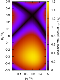
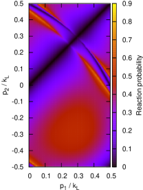
Figure 5: (color online) Elastic scattering rate (left panel) and reaction probability (right panel) for collisions of bosonic molecules in a lattice of depth $u=E_{\rm R}$. Both colliding molecules are in the fundamental energy band.

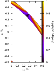
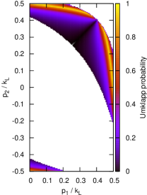
Figure 6: (color online) Umklapp collision probability for bosonic molecules in a lattice of depth $u=E_{\rm R}$ (left panel) and $u=0.2~{}E_{\rm R}$ (right panel). Both colliding molecules are in the fundamental energy band.

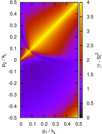
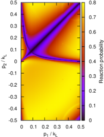
Figure 7: (color online) Elastic scattering factor (left panel) and reaction probability (right panel) for collisions of bosonic molecules in a lattice of depth $u=E_{\rm R}$. Both colliding molecules are in the first excited energy band.

Fig. 7 presents our results for two particles in the first excited energy band. For $u=E_{\rm R}$ the bandwidth is relatively large. As shown in the right panel of the figure this increased mobility results in the reaction probability being large in most of the Brillouin zone. The elastic rate (not shown) presents a structure in the Brillouin zone similar to the reactive one, mostly determined by the velocity factor in definition (3). At variance with the case of the fundamental band we prefer to depict in the left panel the elastic scattering factor $|1-S(qQ\alpha\leftarrow qQ\alpha)|^{2}$. Such factor reaches its maximum for $q\to 0$ ($p_{1}\to p_{2}$) where the elastic scattering matrix element $S\to-1$. In most of the Brillouin zone both inter- and intra-band $\it umklapp$ processes are allowed with up to four channels open. Near the upper and lower right corners of the Brillouin zone scattering is purely elastic. Channel opening takes place along nontrivial lines where the scattering quantities present nonanalytical cusp behaviors. Closer inspection shows for instance that the arched dark line in the left panel and the two bright light lines near the upper and lower right corners are in fact threshold features.

III.2 Influence of the lattice depth

Let us now study the possibility to use an optical lattice to control the molecular reactivity. We fix example single particle quasi-momenta $p_{1}=k_{\rm L}/4$ and $p_{2}=-p_{1}$ such that the reaction probability tends to be large, as can be seen in the right panel of Fig. (5).

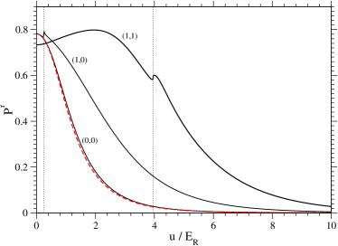
Figure 8: Reaction probability for two bosonic molecules with quasimomentum respectively equal to $p_{1}=k_{\rm L}/4$ and $p_{2}=-k_{\rm L}/4$ as a function of the lattice depth. Labels $(m,n)$ indicate the respective energy zone of each particle. Cusps in the $(1,0)$ and $(1,1)$ reaction probabilities correspond to collision thresholds occurring at the values of $u$ marked by vertical dotted lines. The dashed curve represents the one-channel approximation of Eq. (24).

For particles in the fundamental band, Fig. (8) shows a monotonic decrease of the reaction probability. The drop of $P^{\rm r}$ with $u$ is slower for $u\lesssim E_{\rm R}$ and exponential for large $u$, as dictated by the velocity factor in the numerator of Eq. (24). The figure also shows a good agreement between the exact numerical result and the single-channel approximation of Eq. (24) with interaction and velocity parameters calculated numerically. The behavior of $P^{\rm r}_{\alpha}$ for $\alpha=(10)$ follows a similar pattern, with the exception of a cusp point for $u\simeq 0.25~{}E_{\rm R}$ corresponding to a collision channel closing as neighboring energy bands separate. The value of $P^{\rm r}$ is about one order of magnitude larger as compared to the case where the particles are in the fundamental band. For the case of two particles in the first excited band, the reaction probability presents a non-monotonic behavior before dropping exponentially.

As it can be seen in Fig. (9) the reaction probability for fermionic molecules belonging to the same single-particle energy band is naturally small in the absence of the lattice and is rapidly decreasing with $u$. The situation is drastically different for particles belonging to the fundamental and the first band that show a remarkably high reactivity $P^{\rm r}\simeq 0.4$ for lattices of few recoils. As shown in the figure the two-channel model Eq. (21) with $g$ replaced by $g_{\rm map}$ and the overall minus sign needed for fermions is sufficient to explain with sufficient accuracy this peculiar result. Further insight can be gained by noticing that for weak lattices the CM quasimomentum can be identified with the true CM momentum. Since the latter is conserved under the intermolecular interaction, for $u\ll E_{\rm R}$ one has $g_{12}^{\alpha}\approx 0$. Moreover, our pseudopotential is assumed independent of collision energy, implying that to a good approximation $g_{11}^{\alpha}\approx g_{22}^{\alpha}$. In the tight-binding limit one must obtain $g_{11}^{\alpha}\approx g_{22}^{\alpha}\approx g_{12}^{\alpha}$. As remarked below Eq. (18) $g_{\rm map}$ is large for fermions, magnitude is on the order of $10^{2}\hbar v$ for our physical parameters when $u$ is small. The reaction probability obtained from the two-channel model can therefore be developed to first order in the small parameter $v$. Simple algebra gives

$$P^{\rm r}=\frac{2\hbar v\Re g_{11}^{\alpha}}{(\Re g_{11}^{\alpha})^{2}-(\Re g_{12}^{\alpha})^{2}}.$$ (34)

The steep rise of $P^{\rm R}$ arises from the denominator exponentially vanishing with $u$. In the tight binding limit the reaction probability is ruled by Eq. (33) which gives the expected exponential drop of $P^{\rm r}$ with $v$. Interpolation between these two trends results in the maximum observed in the exact numerical calculation.

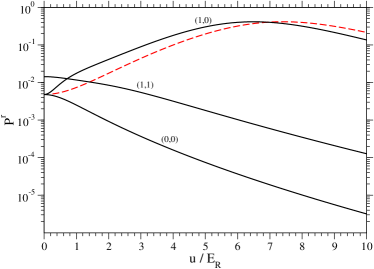
Figure 9: Same as Fig. (8) but for fermions. Note the dramatic increase of the reaction probability for particles in $(1,0)$ bands. Unlike the bosonic case, threshold singularities are not visible on this scale. The dashed curve represents the reaction probability obtained from the two-channel scattering matrix of Eq. (24) with interaction and velocity parameters calculated numerically.

III.3 Effective coupling constant and CM motion

The presence of a lattice breaks up Galilean invariance of flat space. Scattering quantities in a lattice will therefor in general depend on the value of $Q$ or, more precisely, on the CM group velocity $v_{\rm CM}$. Consider an ultracold gas such that in the center-of-mass frame the atom quasimomenta $|p_{i}|\ll k_{\rm L}$. In the laboratory frame $Q$ does not need to be small, a situation that can be experimentally realized by creating an ultracold gas at rest and then adiabatically accelerating or tilting the lattice De Sarlo et al. (2005). We consider here the case of gas with $|q\ll k_{\rm L}|$ and focus on a relatively deep lattice $u=5~{}E_{\rm R}$. The numerically calculated $g^{\rm eff}$ is shown in Fig. (10) for bosonic molecules colliding in the fundamental band. Most striking feature is the drop of both real and imaginary parts of the effective coupling constant for $Q\simeq k_{\rm L}/2$ ($p_{1,2}\simeq k_{\rm L}/4$).

In fact, Eq.(29) results from the scattering solution of a tight binding Hamiltonian with only one symmetrized state of relative motion, equivalent to the Bose-Hubbard model with two particles. This expression predicts an effective coupling constant $g_{\alpha}^{\rm eff}=\bar{g}^{\alpha}$. The momentum dependence of functions $u_{q}$ in Eq. (22) and thus of $\bar{g}$ becomes negligible in the strong lattice limit and the dispersion relation in lattices of depth beyond few recoils is also very accurately represented by the tight binding form. The strong dependence of $\bar{g}$ on quasimomentum depicted in Fig. (10) is therefore unexpected.

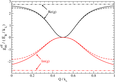
Figure 10: The real and imaginary parts of the effective coupling constant for a lattice depth $u=5.0~{}E_{\rm R}$ computed in the $q\to 0$ limit as a function of the total quasimomentum $Q$. Numerical results (full line) are compared with single channel (dash-dot lines) and two-channel (dashed lines) models (see text).

For the considered lattice depth the tight binding approximation holds with accuracy and umklapp transitions are forbidden for any $Q$. However, one exception exists and is the special value $Q=k_{\rm L}/2$ at which according to Eq. (1) with $n=m$ the relative energy band becomes completely flat. This nonphysical feature stems from the strict ($u\to\infty$) tight binding approximation but in practice the relative motion energy presents for $Q\simeq k_{\rm L}/2$ extrema analogous to the dashed curves shown in Fig. (1) for weaker lattices. In this situation a pair of symmetrized open channels with real $q$ exists. As $Q$ moves away from $k_{\rm L}/2$ one of the two open channels becomes energetically closed ($q$ becomes imaginary) and thus inaccessible to real transitions. However, virtual transitions to such closed channel have a profound influence on the collision.

In order to study this effect on a quantitative ground, let us consider the two-channel scattering matrix Eq. (21) for one open channel and a second channel which can now be either open or become closed with purely imaginary velocity $v_{2}\equiv i{\tilde{v}}_{2}$. In the latter case, the relevant $S$-matrix element becomes

$$S_{11}=\dfrac{(g^{\alpha}_{12})^{2}-(g^{\alpha}_{11}+i\hbar v_{1})(g^{\alpha}_{22}+\hbar{\tilde{v}}_{2})}{(g^{\alpha}_{11}-i\hbar v_{1})(g^{\alpha}_{22}+\hbar{\tilde{v}}_{2})-(g^{\alpha}_{12})^{2}}$$ (35)

which through Eq. (8) gives an effective coupling constant

$$g_{\alpha}^{\rm eff}=\frac{g^{\alpha}_{11}(g^{\alpha}_{22}+\hbar{\tilde{v}}_{2})-(g^{\alpha}_{12})^{2}}{g^{\alpha}_{22}+\hbar{\tilde{v}}_{2}}.$$ (36)

The behavior of the parameters factoring in the former equation is represented in Fig. (11), which shows namely the quantities $\Re g^{\alpha}_{ij}=-\Im g^{\alpha}_{ij}$ and ${\tilde{v}}_{2}=\Im v_{2}$ as a function of $Q$. On one side, one may observe that as predicted by the tight binding approximation the dependence of $g^{\alpha}_{11}$ on the particle quasi-momenta is extremely weak. One the other side, the open-closed $g^{\alpha}_{12}$ and closed-closed $g^{\alpha}_{22}$ channel couplings involve closed-channel wavefunctions that cannot be represented in terms of localized Wannier functions. As a consequence, both $g^{\alpha}_{12}$ and $g^{\alpha}_{22}$ show significant dependence on $Q$ and only tend to $g^{\alpha}_{11}$ for $Q$ near $k_{\rm L}/2$, where the closed and the open channels coalesce. The velocity $v_{2}$ will be real and small in the tiny region of $Q\approx k_{\rm L}/2$ where two open channel exists. Moving away from this region $v_{2}$ first vanishes then evolves continously into a purely imaginary quantity.

The single-channel result $g_{\alpha}^{\rm eff}=g^{\alpha}_{11}$ is only retrieved in the case of weak interactions $|g^{\alpha}_{22}|\ll\hbar|{\tilde{v}}_{2}|$ and $|g^{\alpha}_{12}|^{2}\ll\hbar|{\tilde{v}}_{2}g^{\alpha}_{11}|$. These conditions will however never be satisfied for collisions of atoms with $q\approx 0$ and $Q\approx k_{\rm L}/2$ since ${\tilde{v}}_{2}$ becomes then arbitrarily small. In this case the effect of the closed channel must be taken into account and Eq. (36) predicts indeed the noninteracting behavior with $g_{\alpha}^{\rm eff}\simeq 0$ observed in the full numerical calculation of Fig. (10). Note incidentally that the denominator of Eq. (36) may vanish if $g_{22}^{\alpha}$ is real (i.e. for non reactive species) and equal to ${\tilde{v}}_{2}$, leading to novel resonant behaviors that we plan to study in the near future.

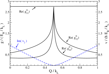
Figure 11: Evolution with $Q$ of the two-channel model parameters in Eq. (21) for a lattice depth $u=5~{}E_{\rm R}$. The vanishing of the velocity parameter $v_{2}$ near $Q=k_{\rm L}/2$ has a strong influence on the collision (see text). The imaginary part of the coupling constant is not shown since for universal reactions one has strictly $\Im g=-\Re g$.

IV Conclusions and perspectives

We have presented a computational algorithm for the calculation of two-body collision properties in an infinite periodic 1D structure. Our computational approach presents distinct advantages since it uses regular and irregular functions computed at fixed collision energy, therefore avoiding a numerically more tedious spectral expansion of the Green’s operator Wouters and Orso (2006). The model allows us to assess quantitatively the expected effect of the lattice in suppressing the reactive collision rates. We also show that for fermionic molecules in different bands the lattice can have the counterintuitive effect of strongly enhancing the reactive processes before suppressing them. A two-channel approach stresses the role of Bloch waves with complex relative quasimomentum in renormalizing the coupling constant for particles in the fundamental band even when the lattice is strong.

In perspective it will be interesting to study lattice-induced resonances in non-reactive systems and, in the spirit of what has been done in three dimensions in Ref. Büchler (2010), to predict the Bose-Hubbard parameters in 1D systems based on an accurate microscopic model. Finally, if a fully quantitative model will be needed in order to compare with experiments, the present reference functions can be used in standard 3D close-coupled models to extract efficiently the scattering observables.