GK Per and EX Hya: Intermediate polars with small magnetospheres

Observed hard X-ray spectra of intermediate polars are determined mainly by the accretion flow velocity at the white dwarf surface, which is normally close to the free-fall velocity. This allows to estimate the white dwarf masses as the white dwarf mass-radius relation $M-R$ and the expected free-fall velocities at the surface are well known. This method is widely used, however, derived white dwarf masses $M$ can be systematically underestimated because the accretion flow is stopped at and re-accelerates from the magnetospheric boundary $R_{\rm m}$, and therefore, its velocity at the surface will be lower than free-fall. To avoid this problem we computed a two-parameter set of model hard X-ray spectra, which allows to constrain a degenerate $M-R_{\rm m}$ dependence. On the other hand, previous works showed that power spectra of accreting X-ray pulsars and intermediate polars exhibit breaks at the frequencies corresponding to the Keplerian frequencies at the magnetospheric boundary. Therefore, the break frequency $\nu_{\rm b}$ in an intermediate polar power spectrum gives another relation in the $M-R_{\rm m}$ plane. The intersection of the two dependences allows, therefore, to determine simultaneously the white dwarf mass and the magnetospheric radius. To verify the method we analyzed the archival Suzaku observation of EX Hya obtaining $M/M_{\odot}=0.73\pm 0.06$ and $R_{\rm m}/R=2.6\pm 0.4$ consistent with the values determined by other authors. Subsequently, we applied the same method to a recent NuSTAR observation of another intermediate polar GK Per performed during an outburst and found $M/M_{\odot}=0.86\pm 0.02$ and $R_{\rm m}/R=2.8\pm 0.2$. The long duration observations of GK Per in quiescence performed by Swift/BAT and INTEGRAL observatories indicate increase of magnetosphere radius $R_{\rm m}$ at lower accretion rates.

1 Introduction

Close binary systems consisting of a normal donor and a white dwarf (WD) accreting through Roche lobe overflow are named cataclysmic variables (CVs, see review in Warner 2003). Intermediate polars (IPs) are a subclass of CVs with moderately magnetized WDs ($B\sim 10^{4}-10^{6}$ G). Central parts of accretion discs in these systems are destroyed by the WD magnetic field within its magnetosphere with radius $R_{\rm m}$. At smaller radii the accreted plasma couples to the field lines and forms a shock wave close to the WD magnetic poles. The shocked plasma is heated up to WD virial temperatures ($kT\sim 10-30$ keV), cools through thermal bremsstrahlung, and settles down to the WD surface. As a result, IPs are bright hard X-ray sources (Revnivtsev et al. 2004a; Barlow et al. 2006; Landi et al. 2009). The hot post-shock region is optically thin and its averaged temperature can be estimated directly from the observed spectrum. The plasma temperature depends only on WD compactness, and therefore provides a direct estimate of the WD mass (Rothschild et al. 1981).

A theory of the post-shock regions (PSR) on WDs was first considered by Aizu (1973) and further developed in several works where the WD gravity, the influence of cyclotron cooling, the dipole geometry of the magnetic field, and the difference between the temperatures of the electron-ion plasma components were taken into account (Fabian et al. 1976; Wu et al. 1994; Cropper et al. 1999; Canalle et al. 2005; Saxton et al. 2007; Hayashi & Ishida 2014a). Some of these models were used to estimate the WD masses in several intermediate polars and polars (Cropper et al. 1998, 1999; Ramsay 2000; Revnivtsev et al. 2004b; Suleimanov et al. 2005; Falanga et al. 2005; Brunschweiger et al. 2009; Yuasa et al. 2010; Hayashi & Ishida 2014b). However, in all these models the accreting plasma was assumed to fall from infinity whereas in reality the magnetospheric radius could be small enough (a few WD radii) to break this assumption. As a consequence the accretion flow will be accelerated to lower velocities and the post-shock region will have lower temperature for the given WD parameters. Therefore, WD masses derived from previous PSR models can be underestimated.

Such possibility has been first suggested by Suleimanov et al. (2005) for GK Per to explain a significant discrepancy between the WD mass estimated using RXTE observations of an outburst and optical spectroscopy. Later Brunschweiger et al. (2009) confirmed this conclusion by estimating the WD mass in GK Per in quiescence. The difference between the estimates of the WD mass in EX Hya obtained using the RXTE observations (0.5 $M_{\odot}$, Suleimanov et al. 2005) and from the optical observations (0.79 $M_{\odot}$, Beuermann & Reinsch 2008) was also attributed to a small magnetospheric radius in this system ($\sim$ 2.7 WD radii, see e.g. Revnivtsev et al. 2011).

Here we present a new set of IP model spectra which for the first time quantitatively account for the finite size of the magnetosphere. The models are calculated for a set of magnetospheric radii (expressed in units of WD radii) assuming a relatively high local mass accretion rate ($>$ 1 g s^-1 cm^-2). Additional cyclotron cooling was ignored as it is not important in such conditions. The model is publicly available and allows direct investigations of the dependence of magnetospheric radius on mass accretion rate in IPs.

A new method of simultaneous determination of the WD mass and the magnetospheric radius is suggested on the base of this set. We propose to add the information about the observed frequency of a break in power spectra of the IP X-ray light curves. Using the spectral fitting and this additional information we can constrain the relative magnetospheric radius together with the WD mass. We verified the method using high quality Suzaku observations of the well studied IP EX Hya, and subsequently applied it to study the spectra of the IP GK Per in outburst and quiescence.

2 The method

The basic commonly accepted physical picture of the X-ray emitting region in intermediate polars is that the matter falls along magnetic field lines onto the WD and forms an adiabatic shock above the surface. The free-fall velocity of the matter ${\rm v}_{\rm ff}$ decreases by a factor of four as it crosses the shock according to the Rankine-Hugoniot relations. The rest kinetic energy transforms to internal gas energy and heats the matter up to the temperature

$$kT_{0}=\frac{3}{16}\mu m_{\rm H}\,{\rm v}_{\rm ff}^{2}=\frac{3}{8}\mu m_{\rm H}\,\frac{GM}{R}\left(1-{r_{\rm m}}^{-1}\right).$$ (1)

Here $M$ and $R$ are the mass and the radius of the WD, $r_{\rm m}=R_{\rm m}/R$ is the relative radius of the magnetosphere, $\mu=0.607$ is the mean molecular weight for a completely ionized plasma with solar chemical composition, and $m_{\rm H}$ and $k$ are the proton mass and the Boltzmann constant. Here we take into account that the matter starts falling from the finite distance $R_{\rm m}$ from the WD. The heated matter settles down to the WD surface in the sub-sonic regime and loses energy by optically thin bremsstrahlung. The cooling due to cyclotron emission is insignificant in intermediate polars due to a relatively weak WD magnetic field and can be ignored. The height of the shock wave above the WD surface is determined by the cooling rate and models of the post-shock region can be accurately computed together with emergent spectra (see next Section).

We note that the observed hard X-ray spectra of intermediate polars can be well approximated with thermal bremsstrahlung. The temperature of the bremsstrahlung $kT_{\rm br}$ is, however, lower in comparison with $kT_{0}$, and a proportional factor $A$ between these temperatures can be found from accurate PSR computations only. The computations and their comparison with the observed X-ray spectra presented later give

$$kT_{\rm br}=A\,kT_{0}\approx 0.64\,kT_{0}.$$ (2)

The WD radius depends on the WD mass, see, e.g. Nauenberg (1972):

$$R=7.8\times 10^{8}\,{\rm cm}\,\left(\left(\frac{1.44}{m}\right)^{2/3}-\left(\frac{m}{1.44}\right)^{2/3}\right)^{1/2},$$ (3)

where $m=M/M_{\odot}$ is the WD mass in units of solar masses. Therefore, Eqs. (1 - 3) define a curve in the $m-r_{\rm m}$ plane, which corresponds to the observed bremsstrahlung temperature $kT_{\rm br}$ (see. Fig. 1). Another curve on the $m-r_{\rm m}$ plane can be obtained from X-ray light curve analysis. Revnivtsev et al. (2009, 2011) showed that power spectra of X-ray pulsars and intermediate polars exhibit a break at the frequency $\nu_{\rm b}$ corresponding to the Kepler frequency at $R_{\rm m}$:

$$\nu_{\rm b}^{2}=\frac{GM}{4\pi^{2}\,R_{\rm m}^{3}}.$$ (4)

An example of the power spectrum with the break obtained for the intermediate polar EX Hya using the observations performed by Suzaku observatory (see Sect. 6.1) is presented in Fig. 2. The curve described by Eq. (4) is also shown in Fig. 1. The intersection of the two curves allows to estimate the WD mass and the magnetospheric radius of the investigated intermediate polar.

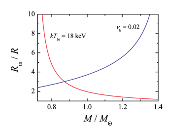
Figure 1: Curves of the constant bremsstrahlung temperature (6) and the constant break frequency (7) on the $m-r_{\rm m}$ plane. Intersection of the curves provides an estimate of the WD mass and the magnetospheric radius.

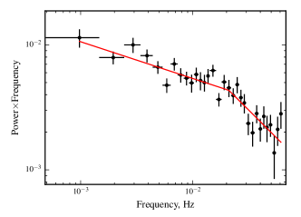
Figure 2: Power spectrum of the 0.5-10 keV X-ray light curve of the EX Hya observed by Suzaku. The break frequency $\nu_{\rm b}=0.021\pm 0.006$ is consistent with value reported by Revnivtsev et al. (2011) using RXTE data.

The Eqs. (1 - 3) and (4) can be simplified using the linear approximation of the WD mass-radius relation presented by Suleimanov et al. (2008)

$$R\approx 1.364\times 10^{9}\,{\rm cm}\,(1-0.59\,m),$$ (5)

which is valid for WD masses in the 0.4-1.2 $M_{\odot}$ range. The resulting relations are

$$m\approx\frac{kT_{\rm br}}{15\,(1-r_{\rm m}^{-1})+0.59\,kT_{\rm br}},$$ (6)

where $kT_{\rm br}$ is measured in keV, and

$$r_{\rm m}\approx 1.5\,\left(\frac{\nu_{\rm b}}{0.02}\right)^{-2/3}\,\frac{m^{1/3}}{1-0.59\,m}.$$ (7)

The accuracy of these relations can be checked using available data. The hard X-ray spectrum of the intermediate polar V1223 Sgr was fitted by a bremsstrahlung spectrum with $kT_{\rm br}\approx 29$ keV (Revnivtsev et al. 2004a). We get $m\approx$ 0.9 using relation (6) with $r_{\rm m}=\infty$, whereas the direct fitting with PSR spectra gave 0.95$\pm$0.05 (Suleimanov et al. 2005). Revnivtsev et al. (2011) found $r_{\rm m}\approx 2.7$ for EX Hya using fixed $m=0.79$ and $\nu_{\rm b}=0.02$. The relation (7) gives $r_{\rm m}\approx$ 2.6.

Thus, relations (6) and (7) allow to evaluate the WD mass and the magnetospheric radius using a simple X-ray spectrum fitted by bremsstrahlung and break frequency in the power spectrum. However, direct fitting of PSR model spectra is necessary for more accurate results. Of course, we use the accurate $M-R$ relation further on and provide the relations above only for convenience.

3 The model of the post-shock region

3.1 Basic equations

The post-shock region can be fully described using the following set of equations (see, for example, Mihalas 1978). The continuity equation is

$${\bf\nabla\cdot}(\rho{\bf v})=0,$$ (8)

where $\rho$ is the plasma density, and $\bf v$ is the vector of the gas velocity. Conservation of momentum for each gas element is described by the vector Euler equation

$$\rho{\bf v\cdot\nabla v}=-{\bf\nabla}P+{\bf f},$$ (9)

where $P$ is the gas pressure (we ignore the radiation pressure here), and ${\bf f}$ is the force density. The energy equation for the gas is

$${\bf\nabla\cdot}\left[\left(\frac{1}{2}\rho{\rm v}^{2}+\varepsilon+P\right){\bf v}\right]={\bf f\cdot v-\nabla\cdot q}.$$ (10)

Here $\varepsilon=(3/2)P$ is the density of internal gas energy. The first term on the right side of the energy equation is the power density, the second term accounts for radiative energy loss (${\bf q}$ is the vector of the radiation flux). These equations must be supplemented by the ideal-gas law

$$P=nkT=\frac{\rho kT}{\mu m_{\rm H}},$$ (11)

where $n$ is the total number density of particles.

Here we consider the one-dimension optically thin flow in a white dwarf gravitational field. Therefore, we substitute the radiation loss term by the local radiative cooling function $\Lambda(\rho,T)$

$${\bf\nabla\cdot q}=\Lambda(\rho,T)=n_{\rm i}n_{\rm e}\Lambda_{\rm N}(T),$$ (12)

where

$$n_{\rm e}=\frac{\rho}{\mu_{\rm e}m_{\rm H}}$$ (13)

is the electron number density, and

$$n_{\rm i}=n-n_{\rm e}=\frac{\rho}{m_{\rm H}}\left(\frac{1}{\mu}-\frac{1}{\mu_{\rm e}}\right)$$ (14)

is the ion number density. Here $\mu_{\rm e}=1.167$ is the mean number of nucleons per electron for fully ionized solar mix plasma. The universal cooling function was computed by many authors and in previous work (Suleimanov et al. 2005) we used $\Lambda_{\rm N}$ computed by Sutherland & Dopita (1993). In the present work we use a more modern cooling function computed by the code APEC (Smith et al. 2001) using the database AtomDB for a solar chemical composition. In the previous work (Suleimanov et al. 2005) the total cooling function was overestimated by factor $\approx 4$, as it was correctly mentioned by Hayashi & Ishida (2014a), because $n^{2}$ instead of $n_{\rm i}\,n_{\rm e}$ was used in Eq. 12. Fortunately, this error did not influence the emergent model spectra and the obtained WD masses (see Appendix). It was corrected in subsequent work (Suleimanov et al. 2008).

We assume that only gravity force operates in the PSR considered here

$${\bf f}=-\frac{GM}{(R+z)^{2}}\,\rho=-g(z)\,\rho.$$ (15)

Here $z$ is geometrical height above the WD surface, and the considered accretion flow settles along $z$.

3.2 Quasi-dipole geometry

We use the approximation of the dipole geometry suggested by Hayashi & Ishida (2014a). They assumed that the PSR cross-section $S$ depends on $z$ as follows: $S\sim z^{n}$. In this case every divergence in hydrodynamical equations can be written as ${\bf\nabla\cdot y}=S^{-1}d(Sy)/dz$:

$$\frac{1}{S}\,\frac{d(S\rho\rm v)}{dz}=0,$$ (16)

$$\rho{\rm v}\,\frac{d{\rm v}}{dz}=-\frac{dP}{dz}-g(z)\,\rho,$$ (17)

and

$$\frac{1}{S}\,\frac{d}{dz}\left[S{\rm v}\left(\frac{1}{2}\rho{\rm v}^{2}+\varepsilon+P\right)\right]=-g(z)\,\rho\,{\rm v}-\Lambda(\rho,T).$$ (18)

If we take $S\sim z^{2}$, we will obtain the well known equations for the spherically symmetric geometry. The dependence $S\sim z^{3}$ mimics the dipole geometry.

Eq. (16) has the integral

$$S\rho\,{\rm v}=a,$$ (19)

where $a$ is the local mass accretion rate at the WD surface, $[a]=$ g s^-1 cm^-2. Using this integral we can replace $\rho$ in the next two Eqs. by $a/S{\rm v}$ and finally we have

$${\rm v}\frac{d{\rm v}}{dz}+\frac{S{\rm v}}{a}\,\frac{dP}{dz}=-g(z),$$ (20)

and

$${\rm v}\frac{dP}{dz}+\gamma\,P\,\frac{d{\rm v}}{dz}+\gamma\frac{P{\rm v}}{S}\,\frac{dS}{dz}=-(\gamma-1)\Lambda(\rho,T),$$ (21)

where $\gamma=5/3$ is the adiabatic index. We note that Eq. (20) coincides with the corresponding equation in Hayashi & Ishida (2014a), with the exception of the energy conservation law. However, our Eq. (21) coincides with the energy equation in Canalle et al. (2005) written for the PSR at the magnetic pole (in this case $\frac{1}{h_{2}}\,\frac{d}{d\omega}=\frac{d}{dz}$), if we take into account that their product $h_{1}h_{3}$ corresponds to our function $S$.

Equations (20) and (21) can be rewritten as follows

$$\frac{d{\rm v}}{dz}=\frac{(\gamma-1)\,S\,\Lambda(\rho,T)+a\,g(z)-\gamma P\,{\rm v}\,dS/dz}{S\gamma\,P-a{\rm v}}$$ (22)

and

$$\frac{dP}{dz}=-g(z)\frac{a}{S{\rm v}}-\frac{a}{S}\,\frac{d{\rm v}}{dz},$$ (23)

where

$$S=\left(\frac{R+z}{R}\right)^{3},$$ (24)

and

$$\frac{dS}{dz}=3\,\frac{(R+z)^{2}}{R^{3}}.$$ (25)

3.3 Method of solution

Equations (22) and (23) can be solved with appropriate boundary conditions. We use a commonly accepted suggestion about a strong adiabatic shock. In particular, at the upper PSR boundary ($z=z_{0}$) we have

$${\rm v_{0}}=-\frac{1}{4}{\rm v_{\rm ff}}(z_{0}),\leavevmode\nobreak\ \leavevmode\nobreak\ \leavevmode\nobreak\ \leavevmode\nobreak\ \leavevmode\nobreak\ \leavevmode\nobreak\ P_{0}=-3\frac{a{\rm v_{0}}}{S(z_{0})},\leavevmode\nobreak\ \leavevmode\nobreak\ \leavevmode\nobreak\ \leavevmode\nobreak\ \leavevmode\nobreak\ T_{0}=3\frac{\mu m_{\rm H}}{k}\,{\rm v}_{0}^{2}$$ (26)

and

$${\rm v}=0$$ (27)

at the WD surface ($z=0$). The free-fall velocity at the upper PSR boundary ${\rm v_{\rm ff}(z_{0})}$ depends on the WD compactness and the inner disc radius, or the magnetosphere radius $R_{\rm m}$

$${\rm v_{\rm ff}}(z_{0})=\sqrt{2GM}\,\left(\frac{1}{R+z_{0}}-\frac{1}{R_{\rm m}}\right)^{1/2}.$$ (28)

Therefore, the input parameters for each PSR model are the WD mass $M$, the local mass accretion rate at the WD surface $a$, and the magnetospheric radius $R_{\rm m}$. We reduced the number of parameters of the model by eliminating the WD radius using the WD mass-radius relation of Nauenberg (1972).

We computed each PSR model using a logarithmically equidistant grid over $z$. We start from the first point with very small $z_{1}=0.1$ cm. We fix the temperature $T_{1}=300\,000$ K and some pressure $P_{1}$ at this point. The corresponding density $\rho_{1}$ and velocity ${\rm v}_{1}$ are found using the mass conservation law (19) and the equation of the state (11). Then Eqs. (22) and (23) are integrated up to the height $z$, where ${\rm v}(z)=0.25\,{\rm v}_{\rm ff}(z)$. At that point the pressure has to be also equal to $-3a{\rm v}(z)/S(z)$. However, the last condition does not hold for the arbitrarily chosen $P_{1}$. Therefore, we find the required pressure at the first point $P_{1}$ in the range 0.1-30  $P_{0}$ by the dichotomy method. Once both aforementioned upper boundary conditions are satisfied with a relative accuracy better than $10^{-8}$, we take the height $z$ as the PSR height $z_{0}$. The results depend slightly on the choice of the starting point (see Fig. 3). In the previous paper (Suleimanov et al. 2005) models were computed starting from the highest PSR point $z_{0}$. Both methods give coincident solutions at $kT>0.5$ keV, but the new one describes the bottom part of the PSR much better.

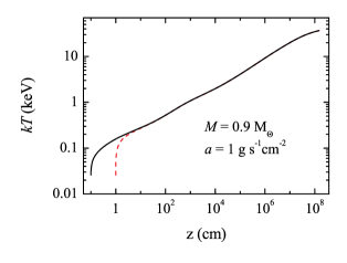
Figure 3: Comparison of the temperature structures of the models computed for two different values of the first model point, $z_{1}=0.1$ cm, solid curve, and $z_{1}=1$ cm, dashed curve.

The code allows to compute models in the cylindrical geometry, too. The computation of a such model with the same parameters, as were used by Hayashi & Ishida (2014a) for one of the models, gives similar results (compare Fig. 4 with figure 2 in Hayashi & Ishida 2014a). We also find a good agreement between our results and those obtained by Canalle et al. (2005) for the dipole geometry (compare Fig. 5 with figure 6 in Canalle et al. 2005)

We note, however, that the results obtained by Hayashi & Ishida (2014a) for the dipole geometry are physically incorrect. They found that the PSR heights are lower in the dipole geometry. However, in the dipole geometry scenario, the plasma cools slowly because of its lower density compared to the cylindrical geometry case. Therefore, the PSR height in the dipole geometry is expected to be higher.

Figure 4: Distributions of temperature and density in the model with $M=M_{\odot}$ and local mass accretion rate $a=1$ g s^-1 cm^-2. See the similar Fig.2 in Hayashi & Ishida (2014a).

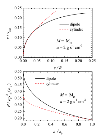
Figure 5: Comparison of the models computed in cylindrical and dipole geometries. This result reproduces Figs. 6 and 4 in the paper by Canalle et al. (2005). Here ${\rm v_{esc}}=\sqrt{2GM/R}$.

3.4 Spectra computations

We computed the PSR model spectra assuming solar abundances and and fully ionized of all the abundant elements in the PSR. This assumption is reasonable at temperatures $kT>$ 1 keV, therefore, the computed spectra are correct at relatively high energies only ($E>3$  keV). At lower energies, the spectra are dominated by numerous emission spectral lines and photo-recombination continua (see, e.g. Canalle et al. 2005). The PSR models are optically thin, and the relative spectra can be calculated by simple integration of the local (at the given height $z$) emissivity coefficients $\eta_{\rm E}=k_{\rm E}\,B_{\rm E}$ and taking into account the dipole geometry

$$F_{\rm E}=\int_{0}^{z_{0}}k_{\rm E}\,B_{\rm E}\,S\,dz,$$ (29)

where $B_{\rm E}$ is Planck function. The free-free opacities $k_{\rm E}$ for the 15 most abundant chemical elements were computed using Kurucz’s code ATLAS (Kurucz 1970, 1993) modified for high temperatures (see details in Ibragimov et al. 2003; Suleimanov & Werner 2007).

Examples of model spectra are presented in Figs. 6 and 7. The first one shows that spectra have a degeneracy with respect to the local mass accretion rate and are almost indistinguishable for any $a>$ 1 g s^-1 cm^-2. The model spectrum computed for $a=0.2$ g s^-1 cm^-2 is, however, slightly softer. Therefore, we can compute the model spectra for every WD mass with one sufficiently high $a$ and it would be sufficient to evaluate the WD mass by fitting its hard X-ray spectrum with the computed PSR model spectra. On the other hand, different inner disc or magnetospheric radii are very important and can influence the WD mass evaluation significantly (Fig. 7).

Using the described method we computed a set of PSR model spectra for a grid of two input parameters, the WD mass $M$ and the relative magnetospheric radius $R_{\rm m}/R$. The maximum PSR temperature $T_{0}$ strongly depends on the factor $1-R/R_{\rm m}$, see Eqs.(26) and (28). Therefore, the equidistant $T_{0}$ sub-grid for a given WD mass has to be proportional to $R_{\rm m}/R\sim N_{\rm max}/N$. We chose the sub-grid with $N_{\rm max}=60$, and $N$ changing from 40 (which corresponds to $R_{\rm m}/R=1.5$) to 1 ($R_{\rm m}/R$=60) . The additional model with $R_{\rm m}/R$=1000 was included to represent the pseudo-infinity magnetospheric radius. The grid was computed for 56 values of WD mass, from 0.3 to 1.4 $M_{\odot}$ with a step of 0.02 $M_{\odot}$, i.e. 2296 models in total. Every PSR model was computed for a fixed mass accretion rate $\dot{M}=10^{16}$  g s^-1 and fixed ratio of the PSR footprint area to the WD surface $f=S_{\rm PSR}/4\pi R^{2}=5\cdot 10^{-4}$. The local mass accretion rate changes from $a\approx 1$  g s^-1 cm^-2 for the lightest WD to $a\approx 70$  g s^-1 cm^-2 for the heaviest WD in accordance with decreasing WD radius. This model grid can be used to estimate the WD mass at fixed $R_{\rm m}/R$ by fitting an IP hard X-ray spectrum. In addition, the fit returns the normalization of the spectrum:

$$K=\frac{fR^{2}}{d^{2}}.$$ (30)

The grid will be distributed as an XSPEC additive table model and publicly available to the scientific community.

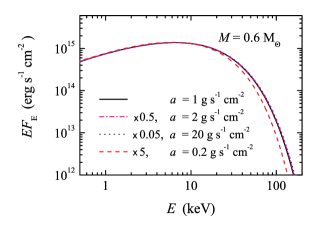
Figure 6: Comparison of model spectra for several local mass accretion rates and a fixed WD mass. Spectra are normalized to the spectrum with $a$  = 1 g s^-1 cm^-2.

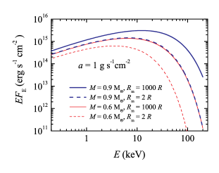
Figure 7: Comparison of model spectra computed for two WD masses, 0.6 (thin curves) and 0.9 (thick curves) $M_{\odot}$ and two relative magnetospheric radii, $R_{\rm m}/R$ = 2 (dashed curves) and 1000 (solid curves). The local mass accretion rate is fixed to $a=1$ g s^-1 cm^-2 for all the computed spectral models.

4 Investigated objects

4.1 EX Hya

This intermediate polar is one of the closest CVs with a distance of $d\approx$ 65 pc and a low accretion luminosity $L_{\rm acc}\approx 2.6\times 10^{32}$ erg s^-1 (Beuermann et al. 2003). The orbital period of EX Hya is relatively short ($P_{\rm orb}$ = 98.26 min), whereas the spin period is relatively long ($P_{\rm s}$ = 67.03 min) in comparison with other intermediate polars. The WD mass in this object is well determined from optical observations ($M/M_{\odot}=0.79\pm 0.03$, Beuermann & Reinsch 2008). Recently, Revnivtsev et al. (2011) found that the magnetospheric radius in EX Hya is small, $R_{\rm m}/R\approx 2.7$. A similar value ($R_{\rm m}/R\approx 2.5$) was found before by Belle et al. (2003). Moreover, Siegel et al. (1989) found the center of the optical radiation in this system is situated at a distance of about $1.5\times 10^{9}$ cm from the WD center. Most probably, this light arises due to irradiation of the inner disc rim with the hard X-ray emission of the PSR. This distance again corresponds to $\sim 2R$ for the $0.8M_{\odot}$ white dwarf. Another evidence of the small magnetospheric radius comes from the permanent white dwarf spin period increasing (Hellier & Sproats 1992). It is possible if the magnetospheric radius is much smaller than the corotation radius, which is indeed a very large for EX Hya ($\sim 50R$). If the corotation radius is close to the magnetospheric one then the intermediate polar will be close to the equilibrium with changing spin-up and spin-down periods (see, e.g. the case of FO Aqr in Patterson et al. 1998).

Such a small magnetospheric radius can explain the small WD masses obtained from the fit of the observed spectra with PSR models (0.5$\pm$0.05 $M_{\odot}$, Suleimanov et al. 2005, and 0.42 $\pm$ 0.02, Yuasa et al. 2010) when an infinity magnetospheric radius was used in the computations. The low absorbed X-ray spectrum of EX Hya allows detailed investigation of the spectral lines (see, e.g. Luna et al. 2015). These properties make EX Hya an ideal target for testing the method of simultaneous determination of the WD mass and the magnetospheric radius proposed in this paper.

4.2 GK Per

The intermediate polar GK Per (Watson et al. 1985) has a very long orbital period ($P_{\rm orb}\approx 1.99$ days) and a K1 sub-giant secondary star (Warner 1976; Crampton et al. 1986; Morales-Rueda et al. 2002). GK Per is also classified as a dwarf nova with very long outbursts ($\approx 50$ days) repeated roughly every 3 years (Šimon 2002). GK Per is also known as Nova Persei 1901 and based on ejecta studies, Warner (1976) determined the distance to GK Per of 460 pc which is consistent with a previous determination (470 pc) made by McLaughlin (1960).

The spin period of the WD in GK Per is relatively short ($P_{\rm s}\approx 351$ s, Watson et al. 1985; Mauche 2004). The pulse profile shape changed from a single-peaked during the outbursts (Hellier et al. 2004) to a two-peaked type in quiescence (Patterson 1991; Ishida et al. 1992). The most likely explanation for these variations is the obscuration of the second WD pole by a dense accretion curtain during the outbursts (Hellier et al. 2004; Vrielmann et al. 2005). During the outbursts, quasi-periodic flux oscillations with a typical time-scale $\sim$ 5000 sec were reported both in X-rays (Watson et al. 1985) and in the emission line spectrum in the optical band (Morales-Rueda et al. 1999).

Analysis of the absorption line spectra of the GK Per secondary during quiescence allowed to determine the stellar mass ratio in the system ($q=0.55\pm 0.21$) and put lower limits for the binary components, $M/M_{\odot}\geq 0.84\pm 0.24$ and $M_{\rm sec}/M_{\odot}\geq 0.48\pm 0.32$ (Morales-Rueda et al. 2002). These values are in accordance with the masses obtained by Crampton et al. (1986), $M/M_{\odot}\approx 0.9\pm 0.2$ and $M_{\rm sec}/M_{\odot}\approx 0.25$. A similar WD mass estimate was obtained by Reinsch (1994), $M/M_{\odot}\geq 0.78$. The large uncertainties in mass determination are mostly due to the poorly constrained inclination of the orbital plane of the system to the line of sight $i$, which was evaluated to be between 73$\degr$ and $\sim$ 50$\degr$ (Reinsch 1994; Morales-Rueda et al. 2002). Warner (1986) claimed $i\sim 75\degr$ using the correlation between the equivalent widths of some emission lines and the inclination angle. This high inclination angle is preferable from our point of view, because the optical emission lines (H_β, HeII 4686, and others) are observed in emission also during the outbursts and no wide absorption wings are observed (Crampton et al. 1986; Morales-Rueda et al. 1999). This behavior is typical for high-inclined CVs with high mass accretion rates (e.g. UX UMa, Neustroev et al. 2011). Therefore, the WD mass is likely close to the lower limit in the allowed region, $M/M_{\odot}\approx 0.9$.

It is also possible to determine the WD masses in old novae by comparing the observed optical light curves of nova outbursts with those predicted by theoretical models. Using this approach Hachisu & Kato (2007) determined for GK Per a WD mass of $M/M_{\odot}=1.15\pm 0.05$. We note, however, that this result depends on the assumed hydrogen mass fraction ($X$=0.54) in the expanded Nova Persei 1901 envelope.

GK Per is a bright hard X-ray source during the outbursts and it was observed by many X-ray observatories including EXOSAT (Watson et al. 1985; Norton et al. 1988), Ginga (Ishida et al. 1992), ASCA (Ezuka & Ishida 1999), RXTE (Hellier et al. 2004; Suleimanov et al. 2005), XMM-Newton (Vrielmann et al. 2005; Evans & Hellier 2007), Chandra (Mauche 2004), INTEGRAL (Barlow et al. 2006; Landi et al. 2009), and Swift / BAT (Brunschweiger et al. 2009). Some of these observations were also used to estimate the WD mass.

The first measurements of the WD mass from X-ray data were based on the cylindrical PSR models (Suleimanov et al. 2005) and the iron line diagnostic method (Ezuka & Ishida 1999). The estimated WD masses turned out to be relatively low (0.59$\pm$0.05 and 0.52 $M_{\odot}$ respectively) and inconsistent with previous estimates based on optical observations ( $\sim 0.9M_{\odot}$ Crampton et al. 1986; Morales-Rueda et al. 2002). Suleimanov et al. (2005) attributed this discrepancy to the fact that the PSR models used to estimate the mass were computed assuming an accretion flow falling from infinity ($R_{\rm m}=\infty$ in Eq. 28) while in reality the co-rotation radius in this system should be smaller than $\sim 10\,R$. Moreover, the magnetospheric radius has to be even smaller during the outburst, as the observed X-ray flux increases by more than a magnitude with respect to quiescence (Ishida et al. 1992). Therefore, the accreting matter is expected to have lower kinetic energy at the WD surface and to reach lower temperatures after the shock, so the WD mass will be underestimated if one assumes that the accretion flow accelerates from infinity.

Brunschweiger et al. (2009) used Swift / BAT observations during the low-flux state of GK Per and took into account the reduction of the kinetic energy. They obtained an improved WD mass value $0.90\pm 0.12\,M_{\odot}$, consistent with estimates based on optical spectroscopy. Nevertheless, recent Suzaku observations of GK Per before and during the latest outburst do not show any significant differences between the spectrum in quiescence just before the outburst and the spectrum on the middle of the flux rise (Yuasa et al. 2016). This behaviour of GK Per has to be investigated further.

In the next sections we re-visit this estimate and investigate the dependence of the magnetospheric radius on X-ray luminosity using the archival RXTE and Swift / BAT observations and the self-consistent PSR models presented in Sect. 3.

5 Observations and data analysis

5.1 Suzaku observations of EX Hya

Suzaku is equipped with the four-module X-ray Imaging Spectrometer (XIS) (Koyama et al. 2007) covering the 0.2-12 keV energy range, and a collimated Hard X-ray Detector (HXD) covering the 10-70 keV and 50-600 keV energy range with PIN and GSO detectors (Kokubun et al. 2007; Takahashi et al. 2007). Suzaku observed EX Hya on Jul 8th 2007 for $\sim 100$ ks (obsid #402001010) with effective exposure of $\sim 75$ ks for XIS and 85 ks for HXD PIN. The source is not detected significantly in the GSO energy band, so we restricted the analysis to XIS and HXD PIN data.

For data reduction we follow the standard procedures and employ default filtering criteria as described in the Suzaku data reduction guide. We use the HEASOFT 6.16 software package with the current instrument calibration files (CALDB version 20151105). For HXD PIN background subtraction we adopted the “tuned” non-X-ray background (NXB) event file provided by the HXD team. We ignored the contribution of cosmic X-ray background (CXB) as it is negligible compared to the source count rate.

5.2 Observations of GK Per

To investigate the properties of the source in outburst we use the recent $\sim 80$ ks long NuSTAR target of opportunity observation performed in April 2015 (obsid 90001008002). We use the HEASOFT 6.16 software package and current instrument calibration files (CALDB version 20151105). We follow the standard procedures described in the instruments data analysis software guide to screen the data and to extract the light curves and spectra. Total useful exposure after screening is $\sim 42$ ks. For timing analysis we combine the data from the two NuSTAR units whereas for spectral analysis we extract and model spectra from the two units separately.

We note that another observation has been performed with NuSTAR in quiescence (Sep 2015, obsid 30101021002), however, the data are not public. Therefore, to assess the source properties outside of the outburst we rely on Swift/BAT (Barthelmy et al. 2005) and INTEGRAL (Winkler et al. 2003) data. The Swift/BAT 70-month survey (Baumgartner et al. 2013) provides mission long spectra and light curves for all detected sources including GK Per (listed as SWIFT J0331.1+4355). The total effective exposure for GK Per is 9.5 Ms. The analysis of the AAVSO light curve of the source shows that three outbursts occurred during the missions lifetime and the averaged spectrum includes these intervals. On the other hand, total duration of outbursts (1.4 Ms) and average flux are comparatively low at $\sim 4.5\times 10^{-11}$ erg cm^-2 s^-1 (in the 20-80 keV energy range), so the quiescent emission is still likely to dominate the average spectrum.

To verify whether this is indeed the case, we also use the data from the INGEGRAL IBIS (Lebrun et al. 2003) instrument including all public observations within 12^∘ from the source and excluding the outburst periods as determined from the BAT light curve (in particular, we exclude intervals when the Swift/BAT flux is greater than 5 mCrab). These results in a total of 1885 INTEGRAL pointings and an effective exposure of $\sim 0.5$ Ms. GK Per is not detected in individual pointings, so we extract the spectrum from the mosaic images obtained using all observations as recommended in the INTEGRAL data reduction guide for faint sources. For data reduction we used the offline software analysis package OSA 10.1 and associated calibration files. The resulting spectrum has factor of two lower flux than the mission long Swift/BAT spectrum (i.e. $2.5\times 10^{-11}$ erg cm^-2 s^-1), but otherwise there is no statistically significant difference in spectral shape. In particular, when fitted with optically thin bremsstrahlung models, the best-fit temperature is 20.1 keV in both cases. Therefore we assume that both ISGRI and BAT spectra are representative of source properties in quiescence and simultaneously fit both with a free cross-normalization factor to account for the flux difference and instrumental discrepancies in absolute flux calibration.

6 Results

6.1 EX Hya

The broadband spectrum presented in Fig. 8 above $\sim 2$ keV is well described with the absorbed PSR model with the WD mass fixed to 0.79 $M_{\odot}$ as found from the binary motion (Beuermann & Reinsch 2008). At lower energies there is a soft excess commonly observed in intermediate polars (Evans & Hellier 2007), which can be accounted for either with a blackbody or APEC with kT $\sim$0.2 keV. Multiple narrow emission lines are known to be present in the soft band as well (Luna et al. 2010) and some are apparent also in the residuals of the XIS spectrum. To account for them we added several gaussians with zero widths and energies fixed to values reported by Luna et al. (2010) based on the high resolution Chandra spectra of the source. We also included a cross-normalization constant fixed to 1.18 for the PIN spectrum (as suggested in data reduction guide for PIN-nominal pointing). Other relevant parameters obtained from the fit are $R_{\rm m}/R=2.06^{+0.05}_{-0.04}$ and $N_{\rm H}=4.1^{+0.1}_{-0.7}\times 10^{21}$ cm^-2.

The hard X-ray continuum ($\gtrsim 3$ keV) is adequately described by the PSR model. The spectra residuals below $\sim 2$ keV are caused by unmodelled line and continuum emission. We conclude, therefore, that the proposed model well describes the X-ray continuum of the source.

The X-ray continuum is mostly sensitive to WD parameters in the hard energy range, hence, the soft part of the spectrum does not actually help to eliminate the model degeneracy between WD mass and magnetosphere radius. In fact, more detailed analysis similar to that by Luna et al. (2010) would be required to derive additional constraints on WD parameters from the soft X-ray spectra. Therefore, due to the strong absorption and lack of broadband quiescent observations, we only considered the spectrum above 20 keV for GK Per (see below). Hereafter we ignore XIS data to estimate the mass of the WD in EX Hya. This approach will allow us to verify whether the proposed method can provide adequate results using hard X-ray data alone.

We used the combined light-curve with time resolution of 8 s from the three XIS units active during the observation to obtain the power spectrum of the source. As shown in Fig. 2, the power spectrum has a break at $\nu_{\rm b}=0.021\pm 0.006$ Hz.

Next, we perform the two-parameter fitting of PIN data using model PSR spectra. The resulting strip, which corresponds to the best fit including formal errors, is shown in the $m-r_{\rm m}$ plane (see Fig. 9). The strip, which corresponds to the break frequency $\nu_{\rm b}$ with the uncertainties (see Fig. 2) is also shown. The crossing of the two regions allows us to find the best fit parameters of EX Hyd, $M/M_{\odot}=0.73\pm 0.06$, and $R_{\rm m}/R=2.6\pm 0.4$. The obtained parameters coincide within errors with the values obtained using other methods (see Sect. 4.1). Therefore, we conclude that the suggested method gives reliable results for EX Hya, and can be used for other intermediate polars.

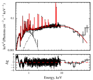
Figure 8: Suzaku spectrum of EX Hya fitted with the PSR model spectrum with $M/M_{\odot}=0.79$ and $R_{\rm m}/R=2$.

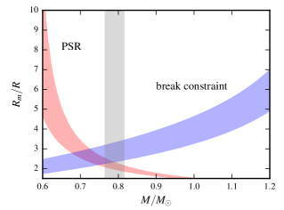
Figure 9: Strips in the $m-r_{\rm m}$ plane obtained using spectral fitting and break frequency in the power spectrum of EX Hya. The vertical strip corresponds to the WD mass known from the optical observations.

6.2 GK Per

6.2.1 Outburst data

Figure 10 shows the NuSTAR background subtracted light curves of the source in two energy bands. The source exhibits correlated variability in both energy bands on timescales of 5-10 ks which resembles the quasi-periodical oscillations (QPOs) reported earlier (Watson et al. 1985; Ishida et al. 1996). However, we do not formally detect the QPOs directly in power spectrum due to the data gaps in the NuSTAR observation which occur on the same timescale.

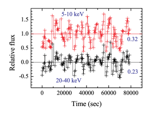
Figure 10: Relative light curves of GK Per in two spectral bands, 5-10 keV and 20-40 keV and time resolution of 351 s. The fluxes in two bands are correlated, but the RMS of the light curve in the soft band is higher (0.32) in comparison with the RMS of the light curve in hard band (0.23).

The most prominent features in the power spectrum of the 3-80 keV lighcurve are the two peaks associated with the spin frequency and the fist harmonic, as well as the break at $\nu_{\rm br}=0.0225\pm 0.004$ (Fig 11).

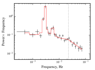
Figure 11: Power spectrum of the X-ray light curve of GK Per observed by NuSTAR. The found break frequency $\nu_{\rm b}=0.0225\pm 0.004$ is marked with the vertical dotted line. The peaks are corresponded to the spin frequency and its first harmonic.

QPOs were previously associated with obscuration of the emission from the white dwarf by bulges in the inner disc (Hellier & Livio 1994). We note that the amplitude of variability in the NuSTAR data decreases with increasing energy (see Fig. 10), which is also consistent with the hypothesis that the flux variability is largely driven by changes in the absorption column. To verify this hypothesis, we fitted the averaged spectrum presented in Fig. 12 with the PSR model modified by partial covering absorber (see, e.g., discussion in Ramsay 2000). First, it is important to emphasize that the higher statistical quality of NuSTAR data makes it clear that this simple model is not really adequate to describe the broadband spectrum of the source below 20 keV. Nevertheless, the spectrum is well described by the model above $\sim 20$ keV.

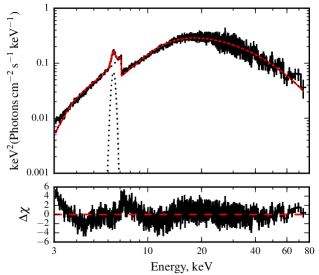
Figure 12: Unfolded NuSTAR spectra of GK Per. The model spectrum was computed for fixed $M/M_{\odot}=0.86$. Other parameters found are $R_{\rm m}/R\approx 2.3$ and $N_{\rm H,1}\approx 1.7\cdot 10^{23}$ cm^-2 . The obtained partial covering parameters are $N_{\rm H,2}\approx 1.24\cdot 10^{24}$ cm^-2 and covering fraction $C_{\rm F}\approx 0.82$, and $\chi^{2}_{\rm dof}\approx 1.75$.

We note also that the light curves folded with the spin period of the white dwarf show no significant dependence on the energy with the pulsed fraction $PF\approx 45\%$ in all the energy bands. Therefore, the absorbing material is likely not located in the immediate vicinity of the WD. In addition, rapid variation of source hardness with time suggests that the absorption is variable on relatively short timescales and that the partial covering absorber is just a useful approximation to account for constantly changing absorption column which is likely caused by the obscuration of the emission region by outer parts of the accretion disk.

Moreover, the hard part of the spectrum is mostly sensitive to the WD parameters whereas the largest fraction of photons are detected in the soft part which is dominated by complex absorption (as expected for the derived absorption column of $10^{23-24}$ cm^-2). We note that while it is possible to describe the broadband spectrum introducing several absorption columns, any ambiguity in modeling of the soft part of the spectrum is likely to affect also the hard part, and thus the derived parameters of the WD simply due to the fact that statistically the soft part is much more important. Therefore, to avoid any potential systematic effects associated with modeling of the soft part of the spectrum we conservatively ignore data affected by the absorption below 20 keV to determine the parameters of the WD.

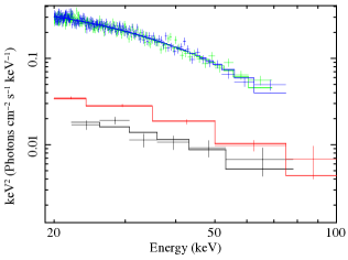
Figure 13: Observed spectra of GK Per used for two-parameter spectral fitting, from top downward: NuSTAR spectrum above 20 keV, Swift/BAT, and INTEGRAL spectra.

The hard X-ray NuSTAR spectrum used to estimate the WD parameters in GK Per is shown in Fig. 13. The resulting strips in the $m-r_{\rm m}$ plane are shown in Fig. 14. The intersection region yields $M/M_{\odot}=0.86\pm 0.02$ and $R_{\rm m}/R\,=\,2.8\pm 0.2$. The value of the mass is consistent with the values determined by other authors (see Sect. 4.2), but our measurement has much better accuracy.

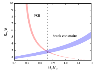
Figure 14: Strips in the $m-r_{\rm m}$ plane obtained using spectral fitting NuSTAR spectrum and break frequency in the power spectrum of GK Per in outburst.

6.2.2 Magnetosphere size

The hard X-ray luminosity of GK Per in quiescence is almost an order of magnitude lower in comparison with the outburst (Fig. 13). Fitting the spectra using the bremsstrahlung model yields $kT_{\rm br}=16.7\pm 0.2$ keV (NuSTAR spectrum in the outburst), $kT_{\rm br}=20.1\pm 0.8$ keV (Swift/BAT averaged spectrum), and $kT_{\rm br}=21^{+4}_{-3}$ keV (INTEGRAL spectrum in the quiescence), i.e. when the luminosity decreases the magnetosphere size increases, thus the temperature increases. To quantify this effect and to obtain the observed dependence $m-r_{\rm m}$ in quiescence we fitted the Swift/BAT and INTEGRAL spectra simultaneously. The result is shown in Fig. 15.

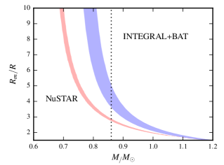
Figure 15: Strips in the $m-r_{\rm m}$ plane obtained using spectral fitting of GK Per in outburst (NuSTAR spectrum) and quiescence (combined Swift/BAT and INTEGRAL spectrum).

It is clear the magnetospheric radius in GK Per indeed increases in quiescence, and equals $4.3^{+2}_{-1}\,R$ for $M=0.86$ $M_{\odot}$. Therefore, we can investigate how the magnetospheric radius depends on the observed X-ray flux and thus the accretion rate (Fig. 16). Here we used the observed flux of GK Per in the 20-80 keV band $F_{20-80}$ as a tracer of the accretion rate. The magnetosphere size is expected to scale as some power of luminosity or accretion rate. We evaluate the exponent $\beta$ in the $r_{\rm m}\sim(F_{20-80})^{\,\beta}$ dependence to $-0.2^{+0.10}_{-0.15}$ using two obtained points on the $r_{\rm m}-F_{20-80}$ plane. Formally, the classical exponent in the equation for the Alfven radius $\beta_{\rm af}=-2/7$ is well consistent with the obtained value (which is rather uncertain due to the low statistics in quiescence). On the other hand, it is interesting to note that similarly to us, Kulkarni & Romanova (2013) found a somewhat lower value than the classical one using 3D MHD simulations for small magnetospheres, with $r_{\rm m}$ in the range 2.5-5:

$$\frac{R_{\rm m}}{R}\approx 1.06\,\left(\frac{\mu_{\rm B}^{4}}{\dot{M}^{2}\,GM\,R^{7}}\right)^{1/10},$$ (31)

where $\mu_{\rm B}\approx BR^{3}$ is the magnetic moment of the WD, and $B$ is the magnetic field strength on its surface. Kulkarni & Romanova (2013) explained this result with compressibility of the magnetosphere and remarked that this effect is less significant for larger magnetospheres. Currently our estimate is rather uncertain due to low statistics in quiescence and not constraining the theory. However, the conclusions by Kulkarni & Romanova (2013) might become testable once better spectra of GK Per at low fluxes are available.

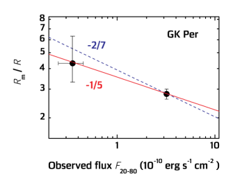
Figure 16: Dependence of the GK Per magnetospheric radius on the observed flux in the 20-80 keV band. The best fit with the slope -1/5 is shown together with the slope -2/7 inferred from the equation for the Alfven radius.

7 Conclusions

We suggested a new method for simultaneous determination of the white dwarf mass and the magnetospheric radius in intermediate polars. The method is based on two independent measurements of the degenerate $M-R_{\rm m}$ dependence using the observed break frequency in the power spectrum (see Revnivtsev et al. 2009, 2011), and the fitting of the hard X-ray spectrum with the newly developed PSR model which takes into account the finite acceleration height of the accretion flow. The two measurements lead to two intersecting regions in the $M/M_{\odot}-R_{\rm m}/R$ plane which allow to estimate the white dwarf mass and the relative magnetospheric radius.

For the spectral fitting procedure, we computed an extensive grid of two-parameter models for hard X-ray spectra of post-shock regions on WD surfaces. We assumed quasi-dipole geometry of the PSR, fixed accretion rate ($\dot{M}=10^{16}$ g s^-1) and a polar region with fixed relative footprint $f=5\times 10^{-4}$ of the WD surface. The cyclotron cooling and difference in temperatures of ion and electron plasmas are currently not taken into account. The WD mass range covered is 0.3 -1.4 $M_{\odot}$ (with steps of 0.02 $M_{\odot}$). The second parameter of the model, the relative magnetospheric radius $r_{\rm m}=R_{\rm m}/R$, changes from 1.5 to 60 with steps proportional to $(1-r_{\rm m}^{-1})$ (we also included a model with $r_{\rm m}=1000$ to ease comparison with previously published results, i.e. the grid includes 41 values of $r_{\rm m}$). The model is implemented in the XSPEC package as an additive table model and accessible to the scientific community.

The method was tested using the well studied intermediate polar EX Hya. We obtained the WD mass of (0.73$\pm 0.06)M_{\odot}$ and magnetospheric radius $R_{\rm m}/R=2.6\pm 0.4$, which are fully consistent with the known WD mass and the magnetosphere size expected for this source. Subsequently we applied the method to another intermediate polar GK Per, which is also a dwarf nova. Large changes of flux during the outburst in GK Per allow not only to estimate the WD mass and the relative magnetosphere size, but to also to investigate the magnetosphere size changes with luminosity.

Using the NuSTAR observation of GK Per during an outburst at the flux level of $F_{\rm 20-80}=3.2\times 10^{-10}$ erg s^-1 cm^-2 in the 20-80 keV range, we estimate the WD mass to $M/M_{\odot}=0.86\pm 0.02$ and $R_{\rm m}/R=2.8\pm 0.2$. The fit to the combined Swift/BAT and INTEGRAL spectra of GK Per in quiescence gives $R_{\rm m}/R=4.3^{+2}_{-1}$ at fixed $M$ and $F_{\rm 20-80}=3.5\times 10^{-11}$ erg s^-1 cm^-2. The derived $R_{\rm m}/R-(F_{\rm 20-80})\,^{\beta}$ dependence with $\beta=-0.2^{+0.10}_{-0.15}$ is consistent with the classical dependence for Alfven radius and with the results obtained by Kulkarni & Romanova (2013) for small magnetospheres from MHD simulations. We note that it could be possible to test the predictions by these authors once the quiescent hard spectra of GK Per with better statistical quality are available.

Appendix A Compare with the previous paper

As mentioned by Hayashi & Ishida (2014a), in the paper Suleimanov et al. (2005) the total number density $n$ was used instead of both the ion number density $n_{\rm i}$ and the electron number density $n_{\rm e}$. That replacement increased the cooling rate in the considered accretion column models approximately four times making a column model four times shorter (see Fig. 17, bottom panel). This led to a different emergent spectrum normalization (four times smaller). Fortunately, the shapes of the computed spectra were not affected (see Fig. 17, top panel). Consequently, the WD masses derived in the Suleimanov et al. (2005) remain correct, because they are determined by the shape of the spectrum only. We note, that this error was found just after the publication, and the spectrum grid used by Brunschweiger et al. (2009) was recomputed with a corrected version of the code. Models computed with Compton scattering taken into consideration (Suleimanov et al. 2008) were also computed using the correct cooling rate.

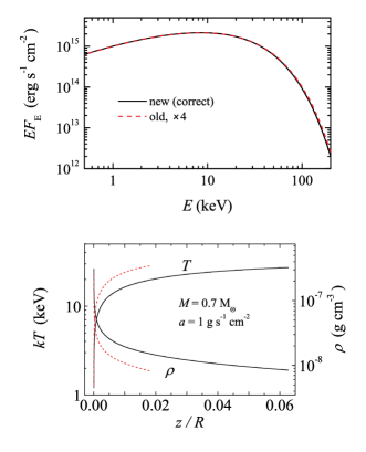
Figure 17: Old and new spectra (top panel) as well as temperature and density stratifications (bottom panel).