Constraining the time evolution of dark energy, curvature and neutrino properties with cosmic chronometers

Abstract

We use the latest compilation of observational Hubble parameter measurements estimated with the differential evolution of cosmic chronometers, in the redshift range $0<z<2$, to place constraints on cosmological parameters. We consider the sample alone and in combination with other state-of-the art cosmological measurements: CMB data from the latest Planck 2015 release, the most recent estimate of the Hubble constant $H_{0}$, a compilation of recent Baryon acoustic oscillation data, and the latest type IA cosmological supernovae sample. Since cosmic chronometers are independent of the assumed cosmological model, we are able to provide constraints on the parameters that govern the expansion history of the Universe in a way that can be used to test cosmological models. In particular, we show that the latest measurements of $H(z)$ obtained with cosmic chronometer from the Baryon Oscillation Spectroscopic Survey (BOSS) survey provide enough constraining power in combination with Planck 2015 data to constrain the time evolution of dark energy, yielding constraints that are competitive with those obtained using Supernovae and/or baryon acoustic oscillations. From late-Universe probes alone ($z<2$) we find that $w_{0}=-0.9\pm 0.18$ and $w_{a}=-0.5\pm 1.7$, and when combining also Planck 2015 data we obtain $w_{0}=-0.98\pm 0.11$ and $w_{a}=-0.30\pm 0.4$. In the theoretical framework, these new constraints imply that nearly all quintessence models are disfavoured by the data; only phantom models or a pure cosmological constant are favoured by the data. This is a remarkable finding as it imposes severe constraints on the nature of dark energy. For the curvature our constraints are $\Omega_{k}=0.003\pm 0.003$, considering also CMB data. We also find that $H(z)$ data from cosmic chronometers are important to constrain parameters that do no affect directly the expansion history, by breaking or reducing degeneracies with other parameters. We find that $N_{\rm eff}=3.17\pm 0.15$, thus excluding the possibility of an extra (sterile) neutrino at more than $5\sigma$, and put competitive limits on the sum of neutrino masses, $\Sigma m_{\nu}<0.27$ eV at 95% confidence level. Finally, we constrain the redshift evolution of dark energy by exploring separately the early and late-Universe, and find a dark energy evolution $w(z)$ consistent with the $\Lambda$CDM model at the 40% level over the entire redshift range $0<z<2$.

1 Introduction

Currently, the $\Lambda$CDM model represents the simplest framework to describe all available cosmological information. Within this model, the Universe has no spatial curvature, the present day energy is mostly constituted of a dark energy component in the form of a cosmological constant, and there are three massless neutrinos. This model can accurately match at the $\sim$percent level current observations with the minimal number of parameters.

One approach to make progress in understanding the nature of dark energy is trying to measure quantities that are independent of the cosmological model. One such technique is to measure directly the expansion history of the Universe: this can be done using massive and passively evolving early-type galaxies as “cosmic chronometers” [1], thus providing standard(-izable) clocks in the Universe. The basic idea underlying this approach is based on the measurement of the differential age evolution as a function of redshift of these chronometers, which provides a direct estimate of the Hubble parameter $H(z)=-1/(1+z)dz/dt\simeq-1/(1+z)\Delta z/\Delta t$. The main strength of this approach is the reliance on the measurement of a differential quantity, $\Delta z/\Delta t$, which provides many advantages in minimizing many common issues and systematic effects (for a detailed discussion, see [2]). There has been significant progress both in the theoretical understanding of the method and control of systematics uncertainties [3, 4] and in the improvement of observational data [2, 5, 6].

Because the cosmic chronometer method measures directly the expansion history, the most interesting parameters to be constrained are those affecting the background evolution, chiefly the evolution of dark energy and the curvature. However, other parameters which from Cosmic Microwave Background data alone show degeneracies with the background evolution, such as neutrino properties, are also affected.

The main aim of this paper is to explore what constraints, independently of the cosmological model (i.e. $\Lambda$CDM-inferred parameters), can be obtained from the the new dataset of $H(z)$ measurements from Ref. [6] both alone and in combination with other data. In particular, we focus on constraints on the time evolution of dark energy, and we demonstrate how early and late-Universe probes give a consistent picture. Further, we demonstrate that the new $H(z)$ data, in combination with the other late-Universe probes, allow for a reconstruction up to 3 free parameters of the time evolution of dark energy, when dark energy is parameterised via a Chebyshev expansion. We also explore the standard Chevallier-Polarski-Linder (CPL) parameterization, providing accurate constraints on dark energy evolution. Despite so much freedom in the form of dark energy as a function of time, we find it to be consistent with a cosmological constant, with only deviations of about 40% permitted in the redshift range $0<z<2$. The rest of the paper is organised as follows. In §2 we present the data, both the $H(z)$ data and the other state-of-the-art cosmological data and in §3 we state our underlying assumptions and the methodological approach. In §4 we present our results, first for the cosmic chronometers data alone, then in comparison with external data sets and finally in combination, discussing our constraints on dark energy time evolution, curvature, and neutrino properties.We conclude in §5.

2 Data

In this analysis, we compare the constraints on cosmological parameters that can be obtained by probes that map the late-time Universe ($z<2$) expansion history, as well as the improvement that can be obtained by combining those with early-time Universe probes. The baseline of our analysis is the Hubble parameter measurements obtained with the cosmic chronometers (hereafter CC) technique, but we consider as well more “standard” probes such as Supernovae Type Ia (hereafter SNe), Baryon Acoustic Oscillation distance measurements (hereafter BAO), and local $H_{0}$ measurements (hereafter $H_{0}$). Early-time Universe probes are the latest Cosmic Microwave Background (CMB) measurements from the Planck mission (hereafter Planck15). We use directly the posterior sampling provided by the Planck collaboration for specific models and for the full combination of temperature and polarisation power spectrum data (in the Planck15 nomenclature TT,TE,EE+lowP). We refer to Ref. [7] for more information. In the following we present the other datasets considered.

Figure 1: Late-time expansion history dataset used in this analysis. The blue lines do not represent a fit to the data, but show the fiducial Planck $\Lambda$CDM cosmology ($H_{0}=67.8$ km/s/Mpc, $\Omega_{m}=0.308$). Lower panels show the residuals of the data with respect to the fiducial Planck cosmology. CC data have been taken from Refs. [8, 9, 2, 10, 5, 6], SNe data from Ref.  [11], and BAO data from Refs. [12, 13, 14].

2.1 Cosmic chronometer dataset

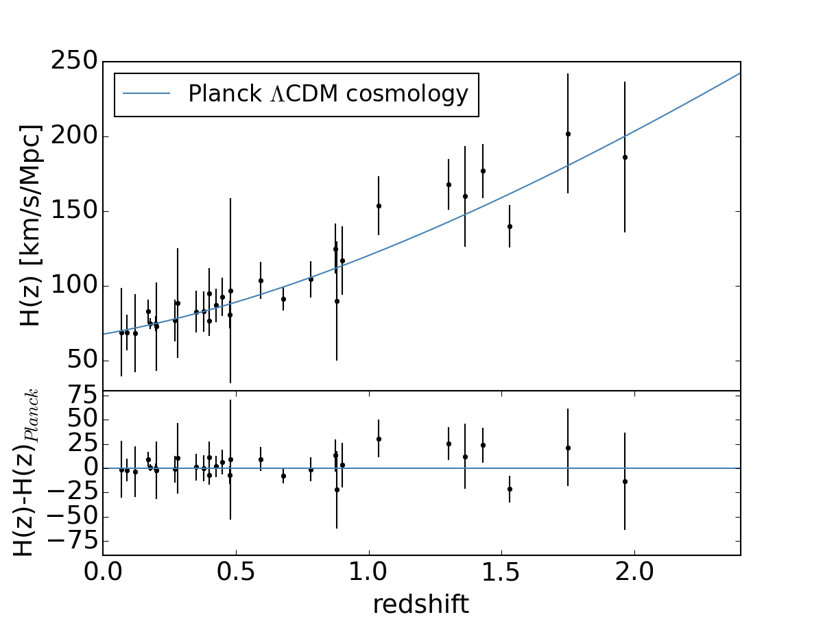
The cosmic chronometers approach to measure $H(z)$ was first introduced in Ref. [1]; it uses relative ages of the most massive and passively evolving galaxies to measure $dz/dt$, from which $H(z)$ is inferred. The latest implementation has been explained in detail in Ref. [2], where the possible sources of uncertainty and related issues are also discussed; we refer to those references for a comprehensive discussion. We consider the compilation of Hubble parameter measurements provided by [6]. It contains the latest updated list of $H(z)$ measurements [8, 9, 2, 10, 5, 6] obtained with the cosmic chronometers approach, comprising of 30 measurements spanning the redshift range $0<z<2$. This sample covers roughly 10 Gyr of cosmic time; the data are presented in Fig. 1. The CC approach to measure $H(z)$ has the desirable feature of being largely independent on assumptions about the cosmological model (besides isotropy and homogeneity); it does, however, rely on the identification of an optimal tracer of the aging of the Universe with redshift (a cosmic chronometer), and the reliable dating of its age. An extended discussion can be found in Ref. [6]. Of particular importance is a possible dependence on the adopted evolutionary stellar population synthesis (EPS) model, which is key in determining the age of the chronometer. In this analysis we used the measurements calibrated on [15] (BC03) EPS models, since they provide the largest dataset to date. However, Ref. [2, 5, 6] provided measurements also with the newest M11 [16] models for a smaller dataset. We explore the dependence of our results on the adopted EPS model in Appendix A.

2.2 Additional datasets

More standard cosmological probes have been also exploited as complementary datasets to this analysis.

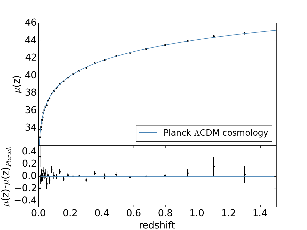
Type 1A supernovae (standard candles) We consider the latest “joint light curves” (JLA) sample [11], comprising 740 SNe Ia from the three year Sloan Digital Sky Survey, Supernova Legacy Survey [17, 18], Hubble Space Telescope [19, 20] and other local experiments (see [21]). Here we use the binned distance modulus provided by Ref. [11], with its associated covariance matrix. It is defined as:

$$\mu_{b}=M+5\log_{10}D_{L}(z)$$ (2.1)

where M is a (nuisance) normalization parameter and $D_{L}(z)$ the luminosity distance at redshift $z$. The luminosity distance at redshift $z$ is related to an integral of the Hubble parameter from redshift $0$ to $z$. As such, it offers sensitivity to the curvature parameter but its integral nature makes it less sensitive than CC to sharp variations in $H(z)$. Also marginalisation over $M$ makes this probe sensitive to the shape of $H(z)$ but not to its overall normalisation (characterised for example by the value at a given redshift like $z=0$, $H_{0}$).

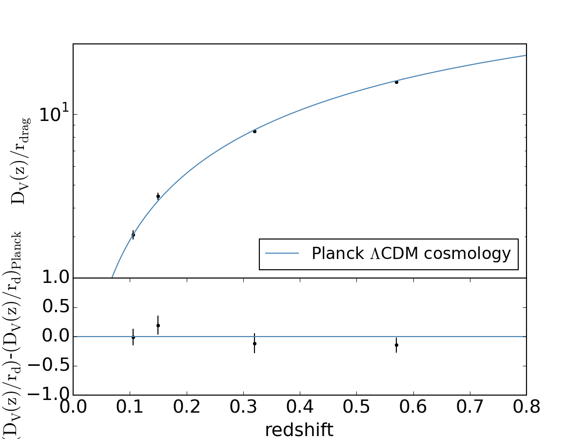
Baryon Acoustic oscillation (standard rulers) Our BAO analysis is based on the (isotropic) acoustic-scale distance ratio $\rm D_{V}(z)/r_{drag}$ where $r_{\rm drag}$ is the sound horizon at radiation drag,

$$D_{V}(z)=\left[(1+z)^{2}D_{A}^{2}(z)\frac{cz}{H(z)}\right]^{1/3}\,,$$ (2.2)

and $D_{A}(z)$ is the angular diameter distance at redshift $z$.

Our compilation comprises the measurements obtained by 6dFGS [12], SDSS Main Galaxy Sample [13] and BOSS LOWZ and CMASS surveys [14] and is similar to the baseline BAO dataset used in Planck 2015 analysis [7]. $D_{V}$ is a combination of an integral of $H(z)$ (through $D_{A}$) and a direct $H(z)$ measurement , but the exquisite measurement of $r_{\rm drag}$ provided by CMB data offers a tight constraint on the overall normalisation of the relation (see e.g., discussion in [22, 23]). BAO measurements have been provided also for other surveys (e.g. Wigglez [24]), or for other subsamples (e.g. galaxy clusters, e.g [25, 26]), but since the covariance between these samples and the dataset used in this analysis has not been estimated, we decided not to use them.

Local $H_{0}$ value. Finally in some cases we also include the local value of $H_{0}$ as measured by Ref. [27] using the recalibration of Ref. [28], which yields $H_{0}=73.0\pm 2.4$ km/s/Mpc. Since there have been claims of tensions between the local $H_{0}$ measurement and the value inferred from early-Universe observations within a $\Lambda$CDM Universe (e.g., [29, 30, 31, 7] and references therein) when including CMB data we will always report results both with and without the $H_{0}$ measurement. In this way the reader can judge wether the inclusion of a possible “discrepant” measurement drives any of the conclusions.

The SNe and BAO data used in this analysis are shown in Fig.1.

3 Methodology

Under the assumptions of isotropy and homogeneity, the metric of space-time of the Universe is fully specified by the Friedmann-$\mathrm{Lema\hat{\i}tre}$- Robertson-Walker one. The most economic $\Lambda$CDM cosmological model can be described by six parameters, but three of them univocally define the background evolution described by the Hubble parameter $H(z)=H_{0}\sqrt{\Omega_{\rm m}(1+z)^{3}+\Omega_{\rm DE}}$. Extensions to this model have been proposed by relaxing one or more of its assumptions, such as flatness, dark energy Equation-of-State (EoS) parameter evolution, number of relativistic species in the Universe, total sum of neutrino masses; in this context, a generic model for the expansion rate of the Universe adopts a generic form for the equation of state parameter of dark energy $w(z)$, and is:

$$H(z)=H_{0}\left\{\Omega_{r}(1+z)^{4}+\Omega_{m}(1+z)^{3}+\Omega_{k}(1+z)^{2}+\Omega_{\rm DE}(1+z)^{3(\int_{0}^{z}\frac{w(z^{\prime})}{(1+z^{\prime})}dz^{\prime})}\right\}^{1/2}\,.$$ (3.1)

where $\Omega_{i}$ denote the energy density parameter for the various species in the Universe (matter, curvature, dark energy and radiation) at $z=0$. Given that the contribution to the total energy due to radiation is not significant at late time where $\Omega_{\rm DE}$ is important, we can safely neglect it; the relation between the energy density parameters is $1=\Omega_{m}+\Omega_{\rm DE}+\Omega_{k}$.

A popular model for the expansion rate of the Universe is given by the CPL [32, 33] parameterisation of the equation of state for dark energy, $w(z)=w_{0}+w_{a}(z/(1+z))$, yielding for the expansion rate:

$$H(z)=H_{0}\left\{\Omega_{r}(1+z)^{4}+\Omega_{m}(1+z)^{3}+\Omega_{k}(1+z)^{2}+\Omega_{\rm DE}(1+z)^{3(1+w_{0}+w_{a})}e^{-3w_{a}\frac{z}{1+z}}\right\}^{1/2}\,.$$ (3.2)

The stronger dependence of $H(z)$ is on the Hubble constant, matter density and curvature parameter, while the dependence on dark energy EoS parameters is less significant, particularly for $w_{a}$ which is the most difficult parameter to be constrained.

We follow two approaches. First, we analyze the constraints that can be put on cosmological parameters, and in particular on dark energy time evolution, with late-Universe probes (i.e. at $z<2$, not considering CMB data), such as CC, SNe and BAO (with and without $H_{0}$), first separately then combined; then we explore how the constraints can be narrowed down by adding early-Universe information from CMB observations. Therefore, we will be able to test how the late and early Universe agrees with each other, being this fully determined within a given cosmological model, like $\Lambda$CDM.

We analyze the goodness of fit of CC, SNe and BAO with a standard $\chi^{2}$ approach. This is possible as the reported errors on the data are Gaussianly distributed. We sample the distribution of parameters with the public python package emcee [34], which is an implementation of the affine-invariant ensemble sampler for Markov chain Monte Carlo (MCMC) proposed by Ref. [35]. For CC we have that:

$$\chi^{2}=\sum\frac{(H_{\rm th}(z)-H_{\rm obs}(z))^{2}}{\sigma_{H_{\rm obs}(z)}^{2}},$$ (3.3)

where $H_{\rm th}(z)$ is taken from Eq. 3.2 and $H_{\rm obs}$ and $\sigma_{H_{\rm obs}}$ from Ref. [6].

For SNe we have:

$$\chi^{2}=(\mu_{b}-M-5\log_{10}(D_{L}(z))^{t}C^{-1}(\mu_{b}-M-5\log_{10}(D_{L}(z)),$$ (3.4)

where $D_{L}$ is the luminosity distance and $C$ the covariance matrix associated with distance modulus measurements $\mu_{b}$ .

For BAO we have:

$$\chi^{2}=\sum\frac{(D_{\rm V,th}(z)/r_{\rm drag}-D_{\rm r,obs}(z))^{2}}{\sigma_{D_{\rm r,obs}(z)}^{2}},$$ (3.5)

where $D_{r}=D_{V}/r_{\rm drag}$, and $D_{\rm V,th}$ is given by Eq. 2.2. When CMB information is not included, $r_{\rm drag}$ is treated as a nuisance parameter i.e., marginalised over.

We considered uniform priors on the following variables: $H_{0}=[50,100]$ km/s/Mpc, $\Omega_{m}=[0.01,0.99]$, $w_{0}=[-3,0]$, $w_{a}=[-5,5]$, $r_{\rm drag}=[100-200]$.

We first explore a flat model ($\Omega_{k}=0$) with the CPL parameterisation for $w(z)$ (fw${}_{0}w_{a}$CDM hereafter) to compare the results with the ones that can be obtained from CMB [7].

Subsequently, to include early time (CMB) constraints we have used the posterior samples provided by the Planck 2015 data release, and importance sampled them with CC measurements, comparing the results with the ones obtained from the combination of Planck15+BAO and Planck15+SNe provided by the Planck team [7].

4 Results

Figure 2: Constraints on a flat $w_{0}w_{a}$CDM cosmology from cosmic chronometers (in green, upper-left panel), SNe (in blue, upper-right panel), BAO data (in red, lower-left panel), and from the combination of the various probes (in grey, lower-right panel) obtained with a MCMC approach. In each panel the contour plots are shown at 68% and 95% confidence level, and the posterior distribution of H₀, $\Omega_{m}$, $w_{0}$ and $w_{a}$, with the 68% and 95% confidence level limits.

We start by discussing the results obtained from late-Universe probes: cosmic chronometer analysis alone, and then in combination with other probes (BAO, SNe). We then combine late-Universe probes with early-Universe observations (CMB) to improve constraints also on parameters that do not have a direct effect on $H(z)$, such as the number of the relativistic species in the Universe $N_{\rm eff}$ and the sum of the neutrino masses $\Sigma m_{\nu}$, by breaking parameter degeneracies.

4.1 Constraints from the late-Universe probes

MARGINALIZED 1D CONSTRAINTS
f$w_{0}w_{a}$CDM model
	H0	$\Omega_{\rm m}$	$w_{0}$	$w_{a}$
CC	$73.2^{+10}_{-8.1}$	$0.31^{+0.09}_{-0.08}$	$-1.46^{+0.77}_{-0.87}$	$-0.5^{+2.6}_{-2.9}$
SNe	–	$0.31^{+0.1}_{-0.15}$	$-0.82^{+0.19}_{-0.26}$	$-0.9^{+1.3}_{-2.1}$
BAO	$70^{+17}_{-14}$	$0.42^{+0.09}_{-0.16}$	$-1.3^{+0.81}_{-0.97}$	$-0.8^{+3.2}_{-2.7}$
CC+SNe+BAO	$67.8\pm 2$	$0.33^{+0.06}_{-0.12}$	$-0.9^{+0.17}_{-0.19}$	$-0.5^{+1.3}_{-2}$

Table 1: Constraints on H₀, $\Omega_{\rm m}$, $w_{0}$ and $w_{a}$ (68% confidence limits) obtained for a flat $\Lambda$CDM cosmology with equation-of-state parameter for dark energy parameterised as $w(z)=w_{0}+w_{a}(z/(1+z))$.

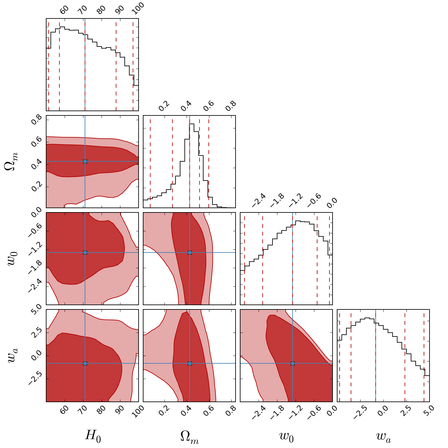
Fig. 2 shows constraints on a flat $w_{0}w_{a}$CDM cosmology using CC, SNe, BAO individually and their combination. Marginalised constraints for each parameter are reported in Tab 1. The poor constraining power on $H_{0}$ of the BAO analysis results from the fact that $r_{\rm drag}$ is treated as a nuisance parameter (i.e. is left as a free parameter, without any CMB prior, and is marginalised over). From this analysis, it is evident that CC and BAO have a similar constraining power in the $w_{0}-w_{a}$ plane, with CC providing better constraints on $H_{0}$ and slightly better constraints on $\Omega_{m}$; SNe, while insensitive to $H_{0}$, provide stringent constraints on the dark energy EoS evolution. Most interestingly, the directions of the degeneracy between parameters in the various probes are different, and hence their combination can provide more stringent constraints, as shown by Fig. 2 bottom right panel. More quantitatively, the constraints obtained with CC are $\sim$70% and $\sim 50$% better than the ones from BAO respectively for $H_{0}$ and $\Omega_{m}$, while just $\sim$8% for the dark energy EoS parameters. The constraints from SNe are better than the ones for CC of a factor $\sim 3.5$ for $w_{0}$, and of $\sim$60% for $w_{a}$, while being worst by $\sim$ 50% on $\Omega_{m}$. The combination of all late-Universe probes yields to a significant improvement of $\sim 40$% on $\Omega_{m}$with respect to SNe alone, and helps to partially remove the degeneracy in the $w_{0}-w_{a}$ plane, improving by $\sim$ 25% the measurements of $w_{0}$.

In order to gain further insights into the time evolution of dark energy, it is useful to explore beyond the two-parameter $w_{0}-w_{a}$ fit. Ideally, one would like to reconstruct $w(z)$ in a non-parametric way; unfortunately, this is not possible (e.g. see Ref. [8]). So, alternatively, one needs to use a parameterisation that is the least possible model dependent. Ref. [8] proposed an expansion with Chebyshev polynomials, $T_{i}$, without any further assumptions on the shape of the dark energy EoS evolution:

$$w(z)=\sum_{i=0}^{N}\omega_{i}T_{i}(x(z))$$ (4.1)

where $T_{i}(x)$ are the Chebyshev polynomials: up to the second order $T_{0}=1$, $T_{1}=x$, $T_{2}=2x^{2}-1$, $x=(2z/z_{max})-1$ and $\omega_{i}$ are the parameters to be constrained by the data.

Figure 3: Constraints for the Chebyshev expansion fit obtained from the combination of cosmic chronometer, SNe and BAO data. In each panel the contour plots are shown at 68% and 95% confidence level, and the posterior distribution of H₀, $\Omega_{m}$, $\omega_{0}$, $\omega_{1}$ and $\omega_{2}$, with the 68% and 95% confidence level limits. For these constraints we assumed a Gaussian prior on $H0=73\pm 2.4$ [27, 28, 36].

MARGINALIZED 1D CONSTRAINTS
Chebyshev expansion
	$\Omega_{\rm m}$	$\omega_{0}$	$\omega_{1}$	$\omega_{2}$
CC+H0	$0.36\pm 0.04$	$-7.6^{+6.2}_{-6.5}$	$-6.1^{+8.7}_{-9.3}$	$-0.2^{+6.3}_{-3.5}$
CC+SNe+BAO+H0 - 1st order	$0.27^{+0.05}_{-0.06}$	$-0.68^{+0.16}_{-0.21}$	$0.53^{+0.30}_{-0.21}$	–
CC+SNe+BAO+H0 - 2nd order	$0.26^{+0.06}_{-0.08}$	$-0.91^{+0.26}_{-0.33}$	$0.13^{+0.47}_{-0.45}$	$-0.46^{+0.4}_{-0.39}$

Table 2: Constraints on H₀, $\Omega_{\rm m}$, and $\omega_{0}$, $\omega_{1}$ and $\omega_{2}$ parameters (from Eq. 4.1) at 68% confidence level obtained from the fit to the Chebyshev expansion of $w(z)$ up to the second order as modeled in Eq. 4.2. For these constraints we assumed a Gaussian prior on $H_{0}=73\pm 2.4$ [27, 28, 36], and hence do not provide the constraints for $H_{0}$.

In this framework, it is possible to write the expansion history (for a flat Universe) as:

$$H(z)=H_{0}(1+z)^{3/2}\sqrt{\Omega_{m}+(1-\Omega_{m})\exp\left(\frac{3}{2}z_{max}\sum_{i=0}^{N}\omega_{i}G_{i}(z)\right)}$$ (4.2)

where the functions $G_{i}$ can be obtained iteratively from the equation $J_{i}=1/nb[(2z/z_{max}-1)^{i}-(-1)^{i}]-(a/b)J_{i-1}$, $J_{0}=1/b\log(1+z)$, $a=1+(z_{max}/2)$ and $b=z_{max}/2$. Up to the first two orders, it can be obtained that $G_{0}=J_{0}$, $G_{1}=J_{1}$ and $G_{2}=2J_{2}-J_{0}$ [8].

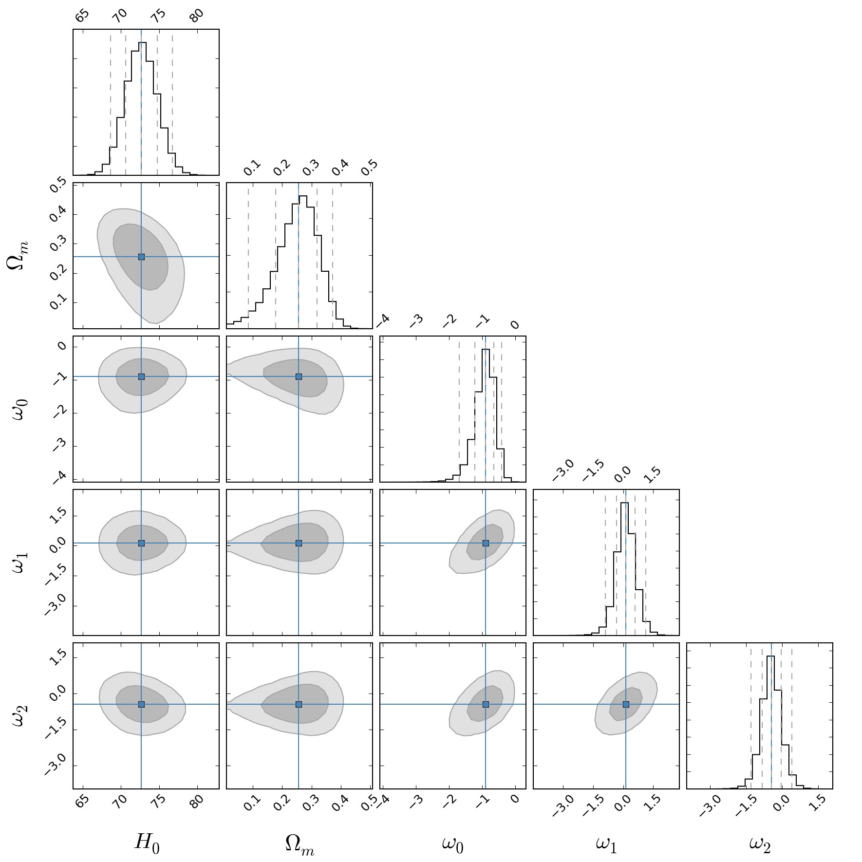
In Tab. 2 we report the results on the constraints of $\omega_{i}$ up to both first and second order obtained by fitting jointly CC, SNe and BAO data to Eq. 4.2, and in Fig. 3 we show the contours for the fit up to the second order. Because of the increased freedom in the EoS parameterisation, in this analysis we always include the $H_{0}$ measurement.

The present-day value of $w$ in this expansion can be estimated as:

$$w_{z=0}=\sum_{i=0}^{N}(-1)^{i}\omega_{i}$$ (4.3)

from which we find from the combined constraints $w_{z=0}=-1.21^{+0.69}_{-0.81}$ with the first order, and $w_{z=0}=-1.5^{+1.4}_{-1.56}$ with the second order expansion.

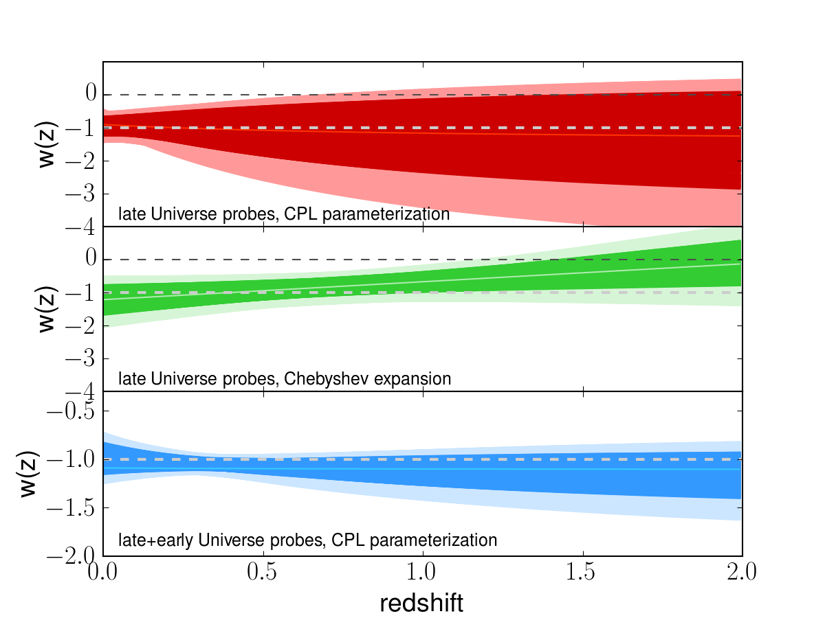
In this analysis by combining SNe and BAO data with the latest CC measurements, we are able to close for the first time the 2$\sigma$ contours on the $\omega_{i}$ parameters up to the second order, significantly improving on previous measurements [8] where unbounded constraints were provided, and only up to the first order. This is an important result, since it provides a measurement of the evolution of dark energy EoS with a completely independent parameterisation. In Fig. 5 we compare the estimated evolution of $w(z)$ with different parameterisations and different datasets combinations, finding, remarkably, results in very good agreement, and compatible with a cosmological constant.

4.2 Combining early-Universe information

Figure 4: Constraints on $\Omega_{\rm m}$, $w_{0}$ and $w_{a}$ for a flat $w_{0}w_{a}$CDM model obtained with different combinations of data sets. Cosmic chronometers and BAO have a similar constraining power in the $w_{0}$-$w_{a}$ plane, as shown in Fig. 2, and the combination of CMB+BAO and CMB+CC provides comparable results. We used $H_{0}73\pm 2.4$ km/s/Mpc from Ref. [27, 28, 36].

MARGINALIZED 1D CONSTRAINTS
f$w_{0}w_{a}$CDM model
	$\Omega_{\rm m}$	$w_{0}$	$w_{a}$
Planck15+BAO	$0.351^{+0.032}_{-0.028}$	$-0.51^{+0.36}_{-0.26}$	$-1.47^{+0.78}_{-1.0}$
Planck15+CC	$0.314^{+0.039}_{-0.052}$	$-0.81\pm 0.40$	$-0.8^{+1.2}_{-1.0}$
Planck15+CC+$H_{0}$	$0.273^{+0.017}_{-0.020}$	$-1.18^{+0.20}_{-0.25}$	$0.01^{+0.63}_{-0.44}$
Planck15+BAO+CC+$H_{0}$	$0.294^{+0.016}_{-0.018}$	$-1.09^{+0.19}_{-0.21}$	$-0.02^{+0.61}_{-0.49}$
Planck15+BAO+SNe+$H_{0}$	$0.3031\pm 0.0093$	$-0.97\pm 0.11$	$-0.34^{+0.45}_{-0.35}$
Planck15+BAO+CC+SNe+$H_{0}$	$0.3032\pm 0.0092$	$-0.98\pm 0.11$	$-0.30^{+0.42}_{-0.34}$

Table 3: Marginalised constraints on $\Omega_{\rm m}$, $\Omega_{\rm DE}$, $\Omega_{\rm k}$, $w_{0}$ and $w_{a}$ at 68% confidence level obtained for a open $\Lambda$CDM cosmology with equation-of-state parameter for dark energy parametrized as $w(z)=w_{0}+w_{a}(z/(1+z))$. We adopted $H_{0}=73\pm 2.4$ km/s/Mpc from Ref. [27, 28, 36].

Figure 5: Reconstruction of the time evolution of dark energy EoS obtained from different probes. Red contours the constraints obtained from late-Universe probes with a CPL parameterisation (see Eq. 3.2 and Tab. 1), green contours show the constraints obtained from late-Universe probes with Chebyshev decomposition up to the first order (see Eq. 4.1 and Tab. 2), and blue contours the constraints obtained adding also CMB information with the CPL parameterisation (see Eq. 3). The darker regions show in each case the 68% confidence level contours, while the light ones the 95% confidence level contours. These constraints assume $H_{0}=73\pm 2.4$ km/s/Mpc, taken from Ref. [27, 28, 36].

CC measurements are extremely useful in breaking CMB parameters degeneracies for models beyond the “minimal” $\Lambda$CDM model. In particular we will show their fundamental importance in models that for allow a time-variability of the dark energy equation of state and for models where CMB constraints show parameter degeneracies with the expansion history.

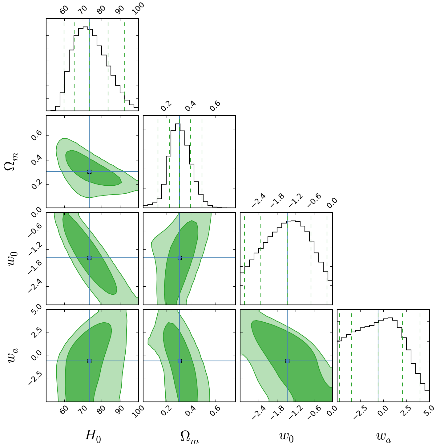
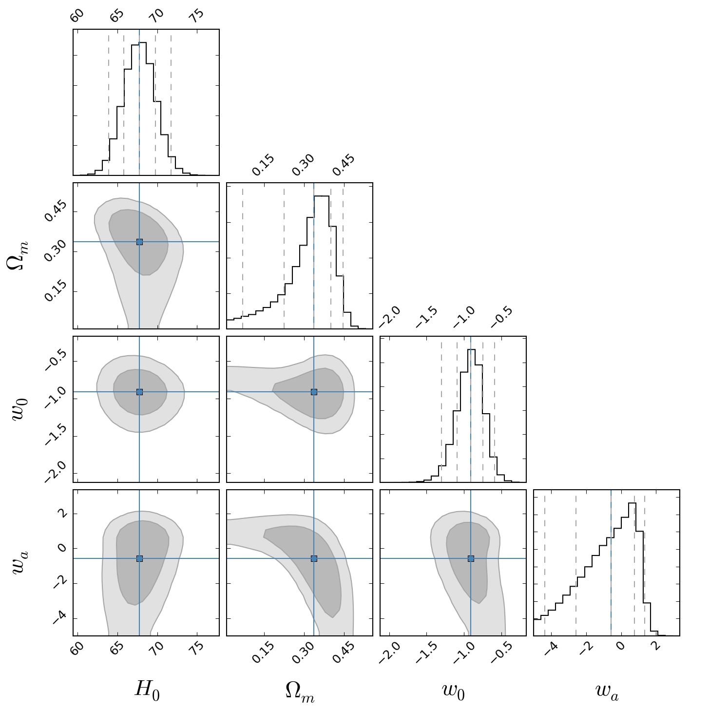
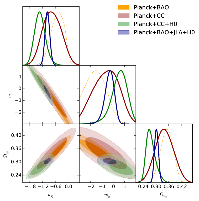
We start extending the “minimal” $\Lambda$CDM where the additional parameter affects directly the late-time expansion history. We first explore a flat $w_{0}w_{a}$CDM model which constraints are presented in Fig. 4 and Tab. 3. For the flat $w_{0}w_{a}$CDM, the base analysis provided by the Planck collaboration include Planck15 and BAO data; as demonstrated in §4.1, CC and BAO have a similar constraining power on the $w_{0}-w_{a}$ plane, hence when combining Planck15+BAO+CC we obtain a little gain in the constraints, still however being able to close the 95% confidence level contours for $w_{a}$. When including also $H_{0}$, the errorbars shrink considerably, and we obtain $w_{0}=-1.09^{+0.19}_{-0.21}$ and $w_{a}=-0.02^{+0.61}_{-0.49}$ (at 68% confidence level); in comparison, the combination Planck15+BAO+CC+SNe+H₀ obtains $w_{0}=-0.98\pm 0.11$ and $w_{a}=-0.30^{+0.42}_{-0.34}$ (at 68% confidence level).

In Fig. 5 we show the evolution of $w(z)$ up to $z=2$ (which is the maximum redshift covered by our datasets) for different parameterisations. We compare the constraints obtained from Chebyshev reconstruction and from a CPL parameterisation from late-Universe probes alone, and from a CPL parameterisation combining also Planck15 measurements. For homogeneity with CPL, we show here the results from Chebyshev reconstruction up to the first order, to compare results with similar degrees of freedom. We find that all the best-fit constraints show deviations from $\Lambda$CDM only up to $\sim 25\%$ up to $z=2$ for the CPL parameterization, and up to $\sim 60$% up to $z=1.5$ for the Chebyshev reconstruction. Quite remarkably, all measurements are compatible at 2$\sigma$ with a constant dark energy EoS $w=-1$ in the entire redshift range. The most accurate measurement is obtained when combining both late- and early-Universe probes together, providing a constraint on $w(z)$ which is consistent with the $\Lambda$CDM model at the 40% level over the entire redshift range $0<z<2$ (at 68% confidence level).

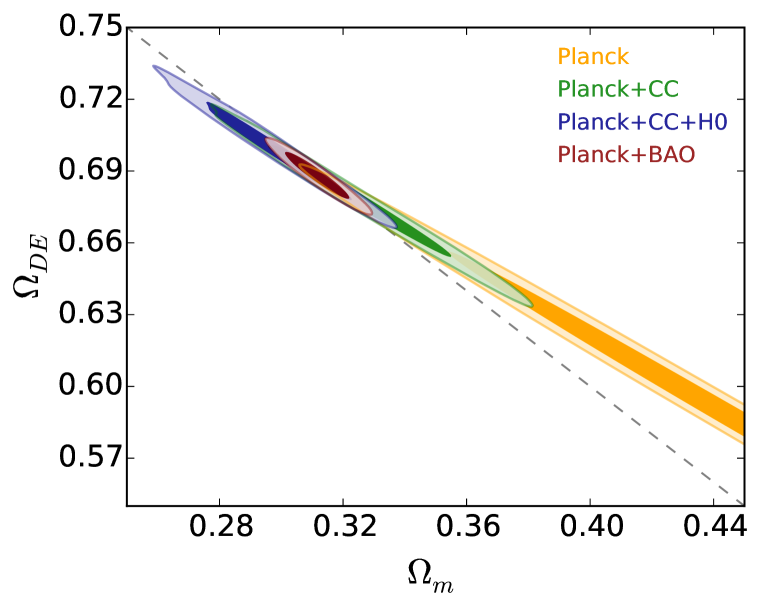
We then consider an open $\Lambda$CDM model, to explore the constraints that can be obtained on curvature from the different probes. The results are shown in Fig. 6 and Tab. 4. We find that cosmic chronometer are fundamental to break the $\Omega_{\rm m}$-$\Omega_{\rm DE}$ degeneracy present in CMB only data, constraining $\Omega_{k}=-0.0030^{+0.0055}_{-0.0042}$. The error bars can be reduced when also the $H_{0}$ data is included, obtaining $\Omega_{k}=0.0028^{+0.0035}_{-0.0031}$. For comparison, BAO data provide a similar result, $\Omega_{k}=0.0002\pm 0.0021$.

Figure 6: Constraints in the $\Omega_{\rm DE}$-$\Omega_{\rm m}$ plane for different data-sets combinations. Note that combining cosmic chronometer data-set with CMB data helps in constraining the contours close to the $\Omega_{\rm k}=0$ region, indicated with the dashed line. Similar results are obtained when combining the BAO with the CMB. We used $H_{0}=73\pm 2.4$ km/s/Mpc from Ref. [27, 28, 36].

MARGINALIZED 1D CONSTRAINTS
o$\Lambda$CDM model
	$\Omega_{\rm m}$	$\Omega_{\rm DE}$	$\Omega_{k}$
Planck15	$0.47^{+0.063}_{-0.086}$	$0.57^{+0.064}_{-0.047}$	$-0.040^{+0.023}_{-0.016}$
Planck15+CC	$0.325^{+0.018}_{-0.023}$	$0.678^{+0.018}_{-0.015}$	$-0.0030^{+0.0055}_{-0.0042}$
Planck15+CC+H0	$0.298\pm 0.015$	$0.699\pm 0.013$	$0.0028^{+0.0035}_{-0.0031}$
Planck15+BAO	$0.3117\pm 0.0070$	$0.6881\pm 0.0065$	$0.0002\pm 0.0021$

Table 4: Constraints on $\Omega_{\rm m}$, $\Omega_{\rm DE}$ and $\Omega_{k}$ at 68% confidence level obtained for an open $\Lambda$CDM cosmology. For $H_{0}$, we considered the value $73\pm 2.4$ km/s/Mpc from Ref. [27, 28, 36].

Figure 7: Constraints on number of effective relativistic species $N_{\rm eff}$ and their total mass $\Sigma m_{\nu}$ obtained with different combination of probes. Note that cosmic chronometers data-set in combination with the CMB provide comparable constraints to those of CMB+BAO. We adopted $H_{0}=73\pm 2.4$ km/s/Mpc from Ref. [27, 28, 36].

MARGINALIZED (95%) 1D CONSTRAINTS
$\Lambda$CDM+$\Sigma m_{\nu}$ model
	$\Sigma m_{\nu}$	$N_{\rm eff}$
Planck15	$<0.577$	$2.93^{+0.39}_{-0.38}$
Planck15+CC	$<0.423$	$3.05^{+0.33}_{-0.32}$
Planck15+CC+$H_{0}$	$<0.269$	$3.17^{+0.29}_{-0.30}$
Planck15+BAO	$<0.222$	$2.99^{+0.37}_{-0.34}$

Table 5: Constraints on $\Sigma m_{\nu}$ (in units of eV) and $N_{\rm eff}$ at 95% confidence level obtained for a flat $\Lambda$CDM cosmology. For $H_{0}$, we assumed a Gaussian prior $73\pm 2.4$ km/s/Mpc from Ref. [27, 28, 36].

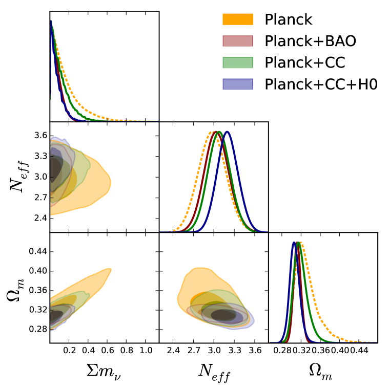
It is possible to constrain neutrino properties from the combination of CMB data with late-Universe measurement of the expansion rate (e.g., see Refs. [37, 38, 27]). In this work, we consider a simple flat $\Lambda$CDM Universe where the effective number of relativistic species $N_{\rm eff}$ is let free, and not fixed to the standard value of $N_{\rm eff}=3.04$; we analyze this model studying the combined dataset of Planck15 and CC and $H_{0}$.

Results are shown in Fig. 7. Planck15+CC have the same constraining power as Planck15+BAO. They restrict $N_{\rm eff}=3.17^{+0.29}_{-0.30}$. Clearly, CC are not able to measure $N_{\rm eff}$ directly, but provide constraints by breaking the degeneracy between the number of relativistic species and the parameters that fix the matter-radiation equality and the expansion history (e.g., see Ref. [38]). We note how, in this case, almost all the statistical power of constraining $N_{\rm eff}$ is given by CC. We then fit a flat $\Lambda$CDM Universe where the total neutrino mass is left as a free parameter, and looked at the constraints on the sum of neutrino masses We obtain a constraint of $M_{\nu}<0.27$ at 95% confidence.

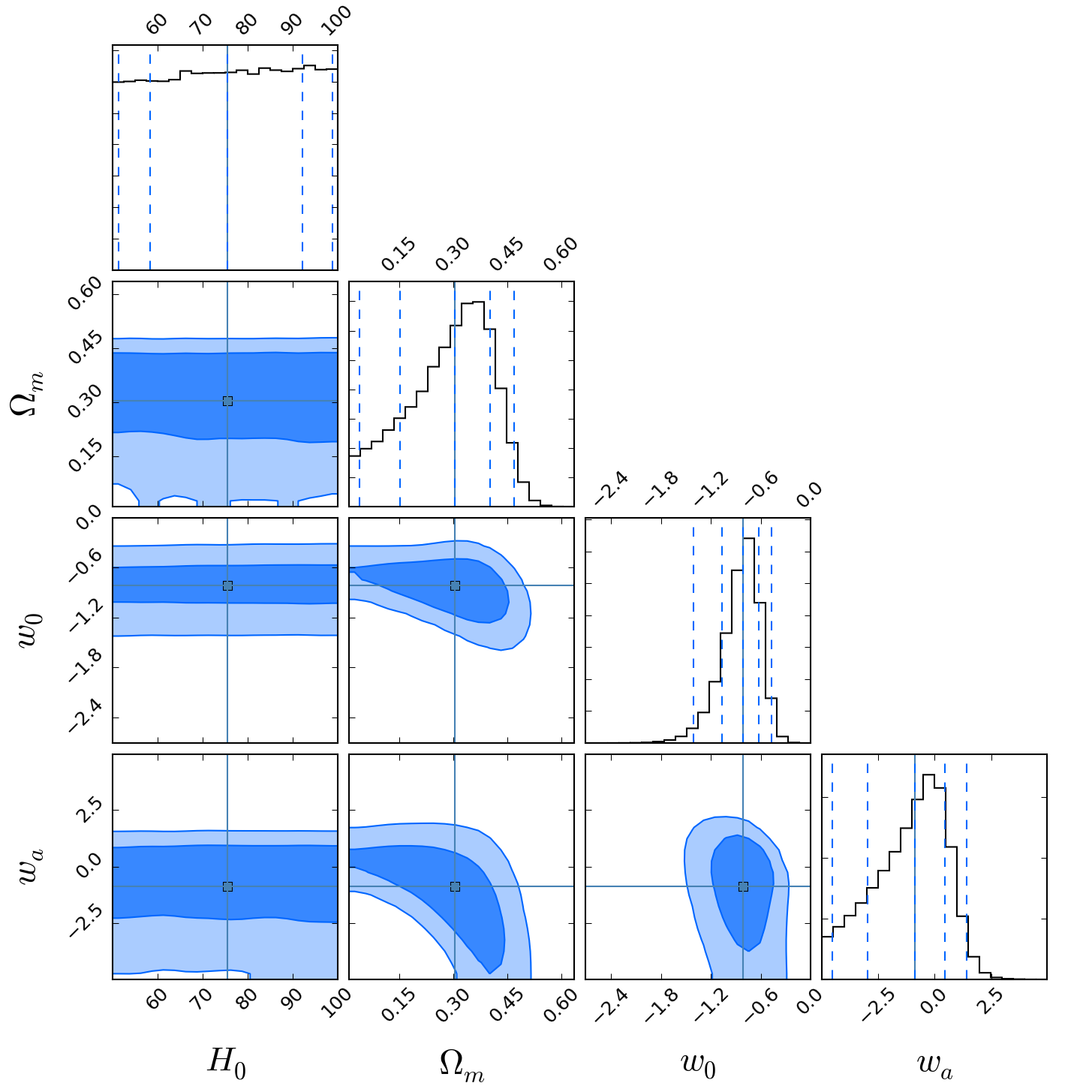
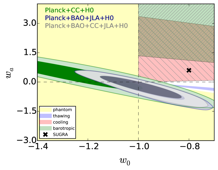
Finally, to exploit the constraining power of our new results in the $w_{0}-w_{a}$ plane, in Fig. 8 we compare our measurements with some theoretical models taken from Ref. [39, 33]. They comprise a large variety of dark energy models, including barotropic models, phantom models, two different quintessence models and a SUGRA model. We refer to Refs. [40, 39] for a comprehensive description of the models. Here we note that thank to the newly analysed data, the 95% allowed region in the $w_{0}-w_{a}$ plane is significantly reduced. The new constraints allow not only to reject at 95% confidence level the barotropic models, but also to exclude almost all quintessence models and the SUGRA model.

Figure 8: Constraints on the time evolution of dark energy equation of state compared to several theoretical models (the brown region is the overlap between barotropic and cooling quintessence models). Models have been taken from Refs. [39, 33]. Dashed lines correspond to the position of the cosmological constant, $(w_{0},w_{a})=(-1,0)$. The Hubble constant considered for these constraints is $H_{0}=73\pm 2.4$ km/s/Mpc from Ref. [27, 28, 36].

5 Conclusions

Measurements of the expansion history are the only direct indication that the Universe is undergoing an accelerated expansion, therefore suggesting that it should be dominated by a dark energy component [6]. Given the magnitude of the implications of the accelerated expansion, it is important to have different, independent and complementary observations of the expansion history.

In this work we have used the latest cosmic chronometers measurements to set constraints on the time evolution of dark energy. We have shown that cosmic chronometers alone are able to set constraints on cosmological parameters comparable to other state-of-the-art late-Universe probes, namely BAO and SNe. However, unlike BAO and SNe, the cosmic chronometer data provide a direct measurements of the expansion rate $H(z)$, without having to assume a cosmological model, and thus can be used to test it.

Remarkably, we find that constraints on dark energy are fully consistent with a cosmological constant up to $z\sim 2$, irrespectively on the assumed parameterisation for $w(z)$, and when combining late- and early-Universe probes we find deviations from the $\Lambda$CDM model smaller than 40% over the entire redshift range $0<z<2$ (at 68% confidence level). In the CPL parameterisation, from the combination of late-Universe probes alone we find $w_{0}=-0.9\pm 0.18$ and $w_{a}=-0.5\pm 1.7$, and when combining also CMB measurements from Planck15 we obtain $w_{0}=-0.98\pm 0.11$ and $w_{a}=-0.30\pm 0.4$. We compared these constraints with a set of theoretical dark energy models, finding that quintessence is disfavoured by the data at high significance, and providing strong constraints on the allowed families of models. We also tightly constrain the geometry of the Universe, obtaining a density parameter for curvature $\Omega_{k}=0.003\pm 0.003$.

Finally, we explored the power of cosmic chronometer in breaking degeneracies between parameters, and hence to constrain quantities that do not directly affects the expansion history of the Universe, namely the number of relativistic species and the total mass of neutrinos. Our measurements provide a value $N_{\rm eff}=3.17\pm 0.15$ that excludes at more than $5\sigma$ the presence of an extra sterile neutrino, putting also a limit on the sum of neutrino masses, $\Sigma m_{\nu}<0.27$ eV at 95% confidence level.

Future surveys such as Euclid [41], WFIRST [42], DESI [43] and LSST [44] will represent the next significant step, providing sub-percent measurements of the dark energy EoS, and giving fundamental insights for our comprehension of the elusive nature of dark energy.

Appendix A Dependence of the results on the assumed evolutionary stellar population synthesis model

Figure 9: Comparison of the results obtained fitting CC with BC03 (in red) and M11 models (in blue). In the left panel are shown the constraints using measurements taken only from Refs. [2, 5, 6], while in the right panel are also considered additional measurements obtained with BC03 model from Refs. [8, 9, 10]. For this constraints, we assumed a Gaussian prior on $H_{0}=73\pm 2.4$ km/s/Mpc from Ref. [27, 28, 36].

MARGINALIZED 1D CONSTRAINTS
f$w_{0}w_{a}$CDM model
	H0	$\Omega_{\rm m}$	$w_{0}$	$w_{a}$
BC03 [2, 5, 6]	$74.2^{+20.1}_{-15.8}$	$0.33^{+0.26}_{-0.19}$	$-1.86^{+1.61}_{-1.1}$	$-0.8^{+5.2}_{-4}$
M11 [2, 5, 6]	$78.3^{+19.6}_{-15.2}$	$0.23^{+0.18}_{-0.18}$	$-1.19^{+1.1}_{-1.5}$	$-1.1^{+4.7}_{-3.7}$
BC03 [8, 9, 2, 10, 5, 6]	$73.4^{+19.2}_{-13.4}$	$0.3^{+0.18}_{-0.2}$	$-1.46^{+1.27}_{-1.4}$	$-0.5^{+4.5}_{-4.2}$
BC03 [2, 5, 6]+H0	–	$0.36^{+0.11}_{-0.23}$	$-1.73^{+0.9}_{-1.1}$	$-0.5^{+4.6}_{-4.2}$
M11 [2, 5, 6]+H0	–	$0.27^{+0.13}_{-0.21}$	$-0.81^{+0.6}_{-0.9}$	$-1.8^{+3.7}_{-3}$
BC03 [8, 9, 2, 10, 5, 6]+H0	–	$0.32^{+0.09}_{-0.21}$	$-1.4^{+0.7}_{-1}$	$-0.3^{+3.4}_{-4.4}$

Table 6: Comparison of the constraints obtained by fitting CC assuming different EPS (BC03 and M11) on H₀, $\Omega_{\rm m}$, $w_{0}$ and $w_{a}$ at 95% confidence level obtained for a flat $\Lambda$CDM cosmology with a CPL parameterisation for the dark energy EoS. In the lower part of the table, we assumed a Gaussian prior on $H_{0}=73\pm 2.4$ km/s/Mpc from Ref. [27, 28, 36], and hence do not provide the constraints for $H_{0}$.

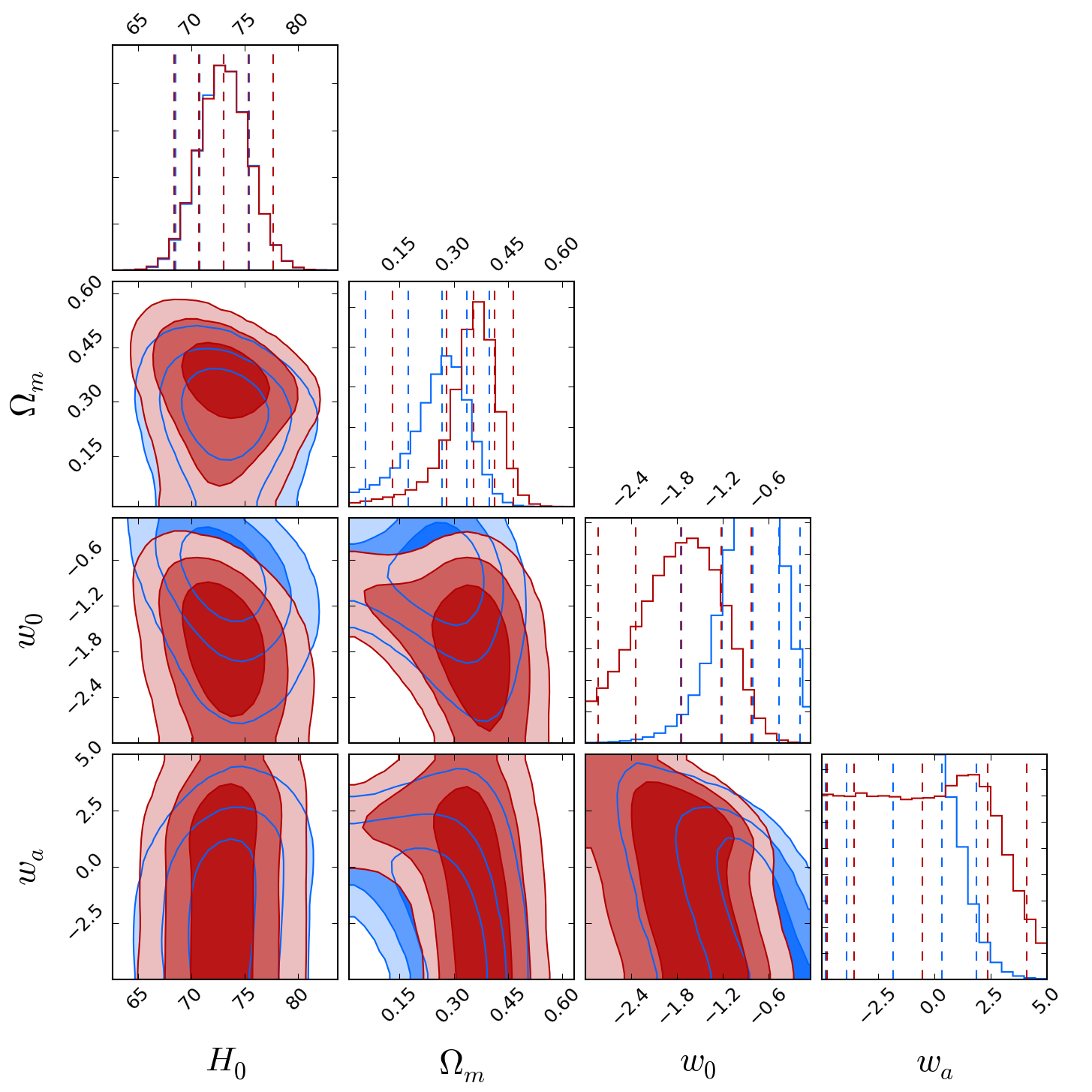
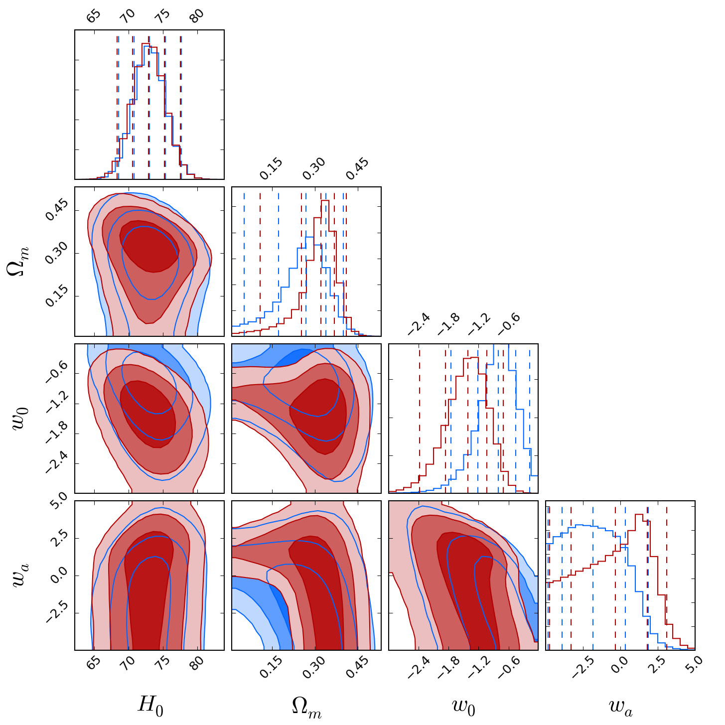
To measure the Hubble parameter $H(z)$ within the CC approach, an evolutionary stellar population synthesis (EPS) model has to be assumed, to calibrate the relation between age and age-related observables used in our analysis. Amongst the models available in literature, so far BC03 [15] and M11 [16] have been used, encompassing significant differences in stellar phases considered, methods implemented and models adopted; for a more detailed discussion, we refer to Ref. [6]. In the following, we explore the dependence of our results on the assumed EPS model.

As a reference, we consider the flat $w_{0}w_{a}$CDM model, and fitted CC data obtained assuming BC03 and M11 models. We performed two different test: firstly, we consider only the limited dataset for which both BC03 and M11 measurements are available [2, 5, 6], and then we compare the result obtained for the full BC03 sample, i.e by considering also the measurements from Refs. [8, 9, 10] (for these measurements, only BC03 constraints are available). We also explored how the constraints change by adding the local measurements of $H_{0}$, as a pivot value for the $H(z)$ relation.

The results are shown in Fig. 9, and reported in Tab. 6. We find no significant difference between the two constraints, with only M11 measurements pointing to a value of $H_{0}$ at higher odds than BC03 with respect to state-of-art measurement. The measurements are still well compatible also when a Gaussian prior on $H_{0}$ is assumed, with the full BC03 dataset providing tighter constraints on cosmological parameters, as expected given the higher number of data available.

We therefore conclude that our measurements are robust, and do not significantly depend on the assumed EPS model.

References

- [1] R. Jimenez and A. Loeb, “Constraining Cosmological Parameters Based on Relative Galaxy Ages,” ApJ, vol. 573, pp. 37–42, July 2002.
- [2] M. Moresco et al., “Improved constraints on the expansion rate of the Universe up to z ~ 1.1 from the spectroscopic evolution of cosmic chronometers,” J. Cosmology Astropart. Phys, vol. 8, p. 6, Aug. 2012.
- [3] M. Moresco, R. Jimenez, A. Cimatti, and L. Pozzetti, “Constraining the expansion rate of the Universe using low-redshift ellipticals as cosmic chronometers,” J. Cosmology Astropart. Phys, vol. 3, p. 45, Mar. 2011.
- [4] M. Moresco, L. Verde, L. Pozzetti, R. Jimenez, and A. Cimatti, “New constraints on cosmological parameters and neutrino properties using the expansion rate of the Universe to z ~ 1.75,” J. Cosmology Astropart. Phys, vol. 7, p. 53, July 2012.
- [5] M. Moresco, “Raising the bar: new constraints on the Hubble parameter with cosmic chronometers at ,” MNRAS, vol. 450, pp. L16–L20, June 2015.
- [6] M. Moresco, L. Pozzetti, A. Cimatti, R. Jimenez, C. Maraston, L. Verde, D. Thomas, A. Citro, R. Tojeiro, and D. Wilkinson, “A 6% measurement of the Hubble parameter at : direct evidence of the epoch of cosmic re-acceleration,” ArXiv e-prints, Jan. 2016.
- [7] Planck Collaboration, P. A. R. Ade, N. Aghanim, M. Arnaud, M. Ashdown, J. Aumont, C. Baccigalupi, A. J. Banday, R. B. Barreiro, J. G. Bartlett, and et al., “Planck 2015 results. XIII. Cosmological parameters,” ArXiv e-prints, Feb. 2015.
- [8] J. Simon, L. Verde, and R. Jimenez, “Constraints on the redshift dependence of the dark energy potential,” Phys. Rev. D, vol. 71, p. 123001, June 2005.
- [9] D. Stern, R. Jimenez, L. Verde, M. Kamionkowski, and S. A. Stanford, “Cosmic chronometers: constraining the equation of state of dark energy. I: H(z) measurements,” J. Cosmology Astropart. Phys, vol. 2, p. 8, Feb. 2010.
- [10] C. Zhang, H. Zhang, S. Yuan, S. Liu, T.-J. Zhang, and Y.-C. Sun, “Four new observational H(z) data from luminous red galaxies in the Sloan Digital Sky Survey data release seven,” Research in Astronomy and Astrophysics, vol. 14, pp. 1221–1233, Oct. 2014.
- [11] M. Betoule, R. Kessler, J. Guy, J. Mosher, D. Hardin, R. Biswas, P. Astier, P. El-Hage, M. Konig, S. Kuhlmann, J. Marriner, R. Pain, N. Regnault, C. Balland, B. A. Bassett, P. J. Brown, H. Campbell, R. G. Carlberg, F. Cellier-Holzem, D. Cinabro, A. Conley, C. B. D’Andrea, D. L. DePoy, M. Doi, R. S. Ellis, S. Fabbro, A. V. Filippenko, R. J. Foley, J. A. Frieman, D. Fouchez, L. Galbany, A. Goobar, R. R. Gupta, G. J. Hill, R. Hlozek, C. J. Hogan, I. M. Hook, D. A. Howell, S. W. Jha, L. Le Guillou, G. Leloudas, C. Lidman, J. L. Marshall, A. Möller, A. M. Mourão, J. Neveu, R. Nichol, M. D. Olmstead, N. Palanque-Delabrouille, S. Perlmutter, J. L. Prieto, C. J. Pritchet, M. Richmond, A. G. Riess, V. Ruhlmann-Kleider, M. Sako, K. Schahmaneche, D. P. Schneider, M. Smith, J. Sollerman, M. Sullivan, N. A. Walton, and C. J. Wheeler, “Improved cosmological constraints from a joint analysis of the SDSS-II and SNLS supernova samples,” A&A, vol. 568, p. A22, Aug. 2014.
- [12] F. Beutler, C. Blake, M. Colless, D. H. Jones, L. Staveley-Smith, L. Campbell, Q. Parker, W. Saunders, and F. Watson, “The 6dF Galaxy Survey: baryon acoustic oscillations and the local Hubble constant,” MNRAS, vol. 416, pp. 3017–3032, Oct. 2011.
- [13] A. J. Ross, L. Samushia, C. Howlett, W. J. Percival, A. Burden, and M. Manera, “The clustering of the SDSS DR7 main Galaxy sample - I. A 4 per cent distance measure at z = 0.15,” MNRAS, vol. 449, pp. 835–847, May 2015.
- [14] L. Anderson, É. Aubourg, S. Bailey, F. Beutler, V. Bhardwaj, M. Blanton, A. S. Bolton, J. Brinkmann, J. R. Brownstein, A. Burden, C.-H. Chuang, A. J. Cuesta, K. S. Dawson, D. J. Eisenstein, S. Escoffier, J. E. Gunn, H. Guo, S. Ho, K. Honscheid, C. Howlett, D. Kirkby, R. H. Lupton, M. Manera, C. Maraston, C. K. McBride, O. Mena, F. Montesano, R. C. Nichol, S. E. Nuza, M. D. Olmstead, N. Padmanabhan, N. Palanque-Delabrouille, J. Parejko, W. J. Percival, P. Petitjean, F. Prada, A. M. Price-Whelan, B. Reid, N. A. Roe, A. J. Ross, N. P. Ross, C. G. Sabiu, S. Saito, L. Samushia, A. G. Sánchez, D. J. Schlegel, D. P. Schneider, C. G. Scoccola, H.-J. Seo, R. A. Skibba, M. A. Strauss, M. E. C. Swanson, D. Thomas, J. L. Tinker, R. Tojeiro, M. V. Magaña, L. Verde, D. A. Wake, B. A. Weaver, D. H. Weinberg, M. White, X. Xu, C. Yèche, I. Zehavi, and G.-B. Zhao, “The clustering of galaxies in the SDSS-III Baryon Oscillation Spectroscopic Survey: baryon acoustic oscillations in the Data Releases 10 and 11 Galaxy samples,” MNRAS, vol. 441, pp. 24–62, June 2014.
- [15] G. Bruzual and S. Charlot, “Stellar population synthesis at the resolution of 2003,” MNRAS, vol. 344, pp. 1000–1028, Oct. 2003.
- [16] C. Maraston and G. Strömbäck, “Stellar population models at high spectral resolution,” MNRAS, vol. 418, pp. 2785–2811, Dec. 2011.
- [17] P. Astier, J. Guy, N. Regnault, R. Pain, E. Aubourg, D. Balam, S. Basa, R. G. Carlberg, S. Fabbro, D. Fouchez, I. M. Hook, D. A. Howell, H. Lafoux, J. D. Neill, N. Palanque-Delabrouille, K. Perrett, C. J. Pritchet, J. Rich, M. Sullivan, R. Taillet, G. Aldering, P. Antilogus, V. Arsenijevic, C. Balland, S. Baumont, J. Bronder, H. Courtois, R. S. Ellis, M. Filiol, A. C. Gonçalves, A. Goobar, D. Guide, D. Hardin, V. Lusset, C. Lidman, R. McMahon, M. Mouchet, A. Mourao, S. Perlmutter, P. Ripoche, C. Tao, and N. Walton, “The Supernova Legacy Survey: measurement of M, Λ and w from the first year data set,” A&A, vol. 447, pp. 31–48, Feb. 2006.
- [18] M. Sullivan, J. Guy, A. Conley, N. Regnault, P. Astier, C. Balland, S. Basa, R. G. Carlberg, D. Fouchez, D. Hardin, I. M. Hook, D. A. Howell, R. Pain, N. Palanque-Delabrouille, K. M. Perrett, C. J. Pritchet, J. Rich, V. Ruhlmann-Kleider, D. Balam, S. Baumont, R. S. Ellis, S. Fabbro, H. K. Fakhouri, N. Fourmanoit, S. González-Gaitán, M. L. Graham, M. J. Hudson, E. Hsiao, T. Kronborg, C. Lidman, A. M. Mourao, J. D. Neill, S. Perlmutter, P. Ripoche, N. Suzuki, and E. S. Walker, “SNLS3: Constraints on Dark Energy Combining the Supernova Legacy Survey Three-year Data with Other Probes,” ApJ, vol. 737, p. 102, Aug. 2011.
- [19] A. G. Riess, L.-G. Strolger, S. Casertano, H. C. Ferguson, B. Mobasher, B. Gold, P. J. Challis, A. V. Filippenko, S. Jha, W. Li, J. Tonry, R. Foley, R. P. Kirshner, M. Dickinson, E. MacDonald, D. Eisenstein, M. Livio, J. Younger, C. Xu, T. Dahlén, and D. Stern, “New Hubble Space Telescope Discoveries of Type Ia Supernovae at z 1: Narrowing Constraints on the Early Behavior of Dark Energy,” ApJ, vol. 659, pp. 98–121, Apr. 2007.
- [20] N. Suzuki, D. Rubin, C. Lidman, G. Aldering, R. Amanullah, K. Barbary, L. F. Barrientos, J. Botyanszki, M. Brodwin, N. Connolly, K. S. Dawson, A. Dey, M. Doi, M. Donahue, S. Deustua, P. Eisenhardt, E. Ellingson, L. Faccioli, V. Fadeyev, H. K. Fakhouri, A. S. Fruchter, D. G. Gilbank, M. D. Gladders, G. Goldhaber, A. H. Gonzalez, A. Goobar, A. Gude, T. Hattori, H. Hoekstra, E. Hsiao, X. Huang, Y. Ihara, M. J. Jee, D. Johnston, N. Kashikawa, B. Koester, K. Konishi, M. Kowalski, E. V. Linder, L. Lubin, J. Melbourne, J. Meyers, T. Morokuma, F. Munshi, C. Mullis, T. Oda, N. Panagia, S. Perlmutter, M. Postman, T. Pritchard, J. Rhodes, P. Ripoche, P. Rosati, D. J. Schlegel, A. Spadafora, S. A. Stanford, V. Stanishev, D. Stern, M. Strovink, N. Takanashi, K. Tokita, M. Wagner, L. Wang, N. Yasuda, H. K. C. Yee, and T. Supernova Cosmology Project, “The Hubble Space Telescope Cluster Supernova Survey. V. Improving the Dark-energy Constraints above z 1 and Building an Early-type-hosted Supernova Sample,” ApJ, vol. 746, p. 85, Feb. 2012.
- [21] A. Conley, J. Guy, M. Sullivan, N. Regnault, P. Astier, C. Balland, S. Basa, R. G. Carlberg, D. Fouchez, D. Hardin, I. M. Hook, D. A. Howell, R. Pain, N. Palanque-Delabrouille, K. M. Perrett, C. J. Pritchet, J. Rich, V. Ruhlmann-Kleider, D. Balam, S. Baumont, R. S. Ellis, S. Fabbro, H. K. Fakhouri, N. Fourmanoit, S. González-Gaitán, M. L. Graham, M. J. Hudson, E. Hsiao, T. Kronborg, C. Lidman, A. M. Mourao, J. D. Neill, S. Perlmutter, P. Ripoche, N. Suzuki, and E. S. Walker, “Supernova Constraints and Systematic Uncertainties from the First Three Years of the Supernova Legacy Survey,” ApJS, vol. 192, p. 1, Jan. 2011.
- [22] A. J. Cuesta, L. Verde, A. Riess, and R. Jimenez, “Calibrating the cosmic distance scale ladder: the role of the sound horizon scale and the local expansion rate as distance anchors,” Mon. Not. Roy. Astron. Soc., vol. 448, no. 4, pp. 3463–3471, 2015.
- [23] E. Aubourg et al., “Cosmological implications of baryon acoustic oscillation measurements,” Phys. Rev., vol. D92, no. 12, p. 123516, 2015.
- [24] E. A. Kazin, J. Koda, C. Blake, N. Padmanabhan, S. Brough, M. Colless, C. Contreras, W. Couch, S. Croom, D. J. Croton, T. M. Davis, M. J. Drinkwater, K. Forster, D. Gilbank, M. Gladders, K. Glazebrook, B. Jelliffe, R. J. Jurek, I.-h. Li, B. Madore, D. C. Martin, K. Pimbblet, G. B. Poole, M. Pracy, R. Sharp, E. Wisnioski, D. Woods, T. K. Wyder, and H. K. C. Yee, “The WiggleZ Dark Energy Survey: improved distance measurements to z = 1 with reconstruction of the baryonic acoustic feature,” MNRAS, vol. 441, pp. 3524–3542, July 2014.
- [25] A. Veropalumbo, F. Marulli, L. Moscardini, M. Moresco, and A. Cimatti, “An improved measurement of baryon acoustic oscillations from the correlation function of galaxy clusters at ,” MNRAS, vol. 442, pp. 3275–3283, Aug. 2014.
- [26] A. Veropalumbo, F. Marulli, L. Moscardini, M. Moresco, and A. Cimatti, “Measuring the distance-redshift relation with the baryon acoustic oscillations of galaxy clusters,” MNRAS, Feb. 2016.
- [27] A. G. Riess, L. Macri, S. Casertano, H. Lampeitl, H. C. Ferguson, A. V. Filippenko, S. W. Jha, W. Li, and R. Chornock, “A 3% Solution: Determination of the Hubble Constant with the Hubble Space Telescope and Wide Field Camera 3,” ApJ, vol. 730, p. 119, Apr. 2011.
- [28] E. M. L. Humphreys, M. J. Reid, J. M. Moran, L. J. Greenhill, and A. L. Argon, “Toward a New Geometric Distance to the Active Galaxy NGC 4258. III. Final Results and the Hubble Constant,” ApJ, vol. 775, p. 13, Sept. 2013.
- [29] G. Efstathiou, “H0 Revisited,” Mon. Not. Roy. Astron. Soc., vol. 440, no. 2, pp. 1138–1152, 2014.
- [30] L. Verde, P. Protopapas, and R. Jimenez, “Planck and the local Universe: Quantifying the tension,” Phys. Dark Univ., vol. 2, pp. 166–175, 2013.
- [31] Planck Collaboration, “Planck 2013 results. XVI. Cosmological parameters,” A&A, vol. 571, p. A16, Nov. 2014.
- [32] M. Chevallier and D. Polarski, “Accelerating Universes with Scaling Dark Matter,” International Journal of Modern Physics D, vol. 10, pp. 213–223, 2001.
- [33] E. V. Linder, “Exploring the Expansion History of the Universe,” Physical Review Letters, vol. 90, p. 091301, Mar. 2003.
- [34] D. Foreman-Mackey, D. W. Hogg, D. Lang, and J. Goodman, “emcee: The MCMC Hammer,” PASP, vol. 125, pp. 306–312, Mar. 2013.
- [35] J. Goodman and J. Weare, “Ensamble samplers with affine invariance,” Commun. Appl. Math. Comput. Sci., vol. 5, pp. 65–8–, 2010.
- [36] A. J. Cuesta, M. Vargas-Magaña, F. Beutler, A. S. Bolton, J. R. Brownstein, D. J. Eisenstein, H. Gil-Marín, S. Ho, C. K. McBride, C. Maraston, N. Padmanabhan, W. J. Percival, B. A. Reid, A. J. Ross, N. P. Ross, A. G. Sánchez, D. J. Schlegel, D. P. Schneider, D. Thomas, J. Tinker, R. Tojeiro, L. Verde, and M. White, “The clustering of galaxies in the SDSS-III Baryon Oscillation Spectroscopic Survey: Baryon Acoustic Oscillations in the correlation function of LOWZ and CMASS galaxies in Data Release 12,” ArXiv e-prints, Sept. 2015.
- [37] B. A. Reid, L. Verde, R. Jimenez, and O. Mena, “Robust neutrino constraints by combining low redshift observations with the CMB,” J. Cosmology Astropart. Phys, vol. 1, p. 003, Jan. 2010.
- [38] F. De Bernardis, A. Melchiorri, L. Verde, and R. Jimenez, “The cosmic neutrino background and the age of the Universe,” J. Cosmology Astropart. Phys, vol. 3, p. 020, Mar. 2008.
- [39] V. Barger, E. Guarnaccia, and D. Marfatia, “Classification of dark energy models in the (w,w) plane,” Physics Letters B, vol. 635, pp. 61–65, Apr. 2006.
- [40] R. R. Caldwell and E. V. Linder, “Limits of Quintessence,” Physical Review Letters, vol. 95, p. 141301, Sept. 2005.
- [41] R. Laureijs, J. Amiaux, S. Arduini, J. . Auguères, J. Brinchmann, R. Cole, M. Cropper, C. Dabin, L. Duvet, A. Ealet, and et al., “Euclid Definition Study Report,” ArXiv e-prints, Oct. 2011.
- [42] D. Spergel, N. Gehrels, J. Breckinridge, M. Donahue, A. Dressler, B. S. Gaudi, T. Greene, O. Guyon, C. Hirata, J. Kalirai, N. J. Kasdin, W. Moos, S. Perlmutter, M. Postman, B. Rauscher, J. Rhodes, Y. Wang, D. Weinberg, J. Centrella, W. Traub, C. Baltay, J. Colbert, D. Bennett, A. Kiessling, B. Macintosh, J. Merten, M. Mortonson, M. Penny, E. Rozo, D. Savransky, K. Stapelfeldt, Y. Zu, C. Baker, E. Cheng, D. Content, J. Dooley, M. Foote, R. Goullioud, K. Grady, C. Jackson, J. Kruk, M. Levine, M. Melton, C. Peddie, J. Ruffa, and S. Shaklan, “Wide-Field InfraRed Survey Telescope-Astrophysics Focused Telescope Assets WFIRST-AFTA Final Report,” ArXiv e-prints, May 2013.
- [43] M. Levi, C. Bebek, T. Beers, R. Blum, R. Cahn, D. Eisenstein, B. Flaugher, K. Honscheid, R. Kron, O. Lahav, P. McDonald, N. Roe, D. Schlegel, and representing the DESI collaboration, “The DESI Experiment, a whitepaper for Snowmass 2013,” ArXiv e-prints, Aug. 2013.
- [44] LSST Science Collaboration, P. A. Abell, J. Allison, S. F. Anderson, J. R. Andrew, J. R. P. Angel, L. Armus, D. Arnett, S. J. Asztalos, T. S. Axelrod, and et al., “LSST Science Book, Version 2.0,” ArXiv e-prints, Dec. 2009.