Waveform Design for Wireless Power Transfer

Abstract

Far-field Wireless Power Transfer (WPT) has attracted significant attention in recent years. Despite the rapid progress, the emphasis of the research community in the last decade has remained largely concentrated on improving the design of energy harvester (so-called rectenna) and has left aside the effect of transmitter design. In this paper, we study the design of transmit waveform so as to enhance the DC power at the output of the rectenna. We derive a tractable model of the non-linearity of the rectenna and compare with a linear model conventionally used in the literature. We then use those models to design novel multisine waveforms that are adaptive to the channel state information (CSI). Interestingly, while the linear model favours narrowband transmission with all the power allocated to a single frequency, the non-linear model favours a power allocation over multiple frequencies. Through realistic simulations, waveforms designed based on the non-linear model are shown to provide significant gains (in terms of harvested DC power) over those designed based on the linear model and over non-adaptive waveforms. We also compute analytically the theoretical scaling laws of the harvested energy for various waveforms as a function of the number of sinewaves and transmit antennas. Those scaling laws highlight the benefits of CSI knowledge at the transmitter in WPT and of a WPT design based on a non-linear rectenna model over a linear model. Results also motivate the study of a promising architecture relying on large-scale multisine multi-antenna waveforms for WPT. As a final note, results stress the importance of modeling and accounting for the non-linearity of the rectenna in any system design involving wireless power.

I Introduction

Wireless Power Transfer (WPT) via radio-frequency radiation has a long history that is nowadays attracting more and more attention. RF radiation has indeed become a viable source for energy harvesting with clear applications in Wireless Sensor Networks (WSN) and Internet of Things (IoT) [2]. The major challenge facing far-field wireless power designers is to find ways to increase the DC power level at the output of the rectenna without increasing the transmit power, and for devices located tens to hundreds of meters away from the transmitter. To that end, the vast majority of the technical efforts in the literature have been devoted to the design of efficient rectennas, a.o. [2, 3, 4]. A rectenna harvests ambient electromagnetic energy, then rectifies and filters it (using a diode and a low pass filter). The recovered DC power then either powers a low power device directly, or is stored in a super capacitor for higher power low duty-cycle operation.

Interestingly, the overall RF-to-DC conversion efficiency of the rectenna is not only a function of its design but also of its input waveform. However, the waveform design has received less attention [5, 6, 7]. In [5, 6], a multisine signal excitation is shown through analysis, simulations and measurements to enhance the DC power and RF-to-DC conversion efficiency over a single sinewave signal. In [7], various input waveforms (OFDM, white noise, chaotic) are considered and experiments show that waveforms with high peak to average power ratio (PAPR) increase RF-to-DC conversion efficiency. Even though those papers provide some useful insights into the impact of waveform design onto WPT performance, there are many limitations in the WPT waveform design literature: 1) there has not been any formal tool to design and optimize waveforms for WPT so far, 2) multipath fading (well known in wireless communications) has been ignored despite its tremendous impact on the received waveform at the input of the rectenna, 3) the Channel State Information (CSI) is assumed unknown to the transmitter, 4) the transmitter is commonly equipped with a single antenna and 5) a single rectenna is considered.

In this paper we address the important problem of waveform design for WPT and tackle all the aforementioned limitations. We focus on multisine waveforms due to their tractability and usefulness in wireless communication systems. The contributions of the paper are summarized as follows.

First, we introduce a simple and tractable analytical model of the rectenna non-linearity through the second and higher order terms in the Taylor expansion of the diode characteristics. Comparison is made with a linear model, first introduced in [8] and nowadays popular in Simultaneous Wireless Information and Power Transfer (SWIPT), e.g. [9] and subsequent works, that only accounts for the second order term.

Second, assuming perfect CSI at the Transmitter (CSIT) can be attained and making use of the rectenna model, we design multi-antenna multisine WPT waveform for transmission over a multipath channel. We formulate an optimization problem to adaptively change the waveform weights as a function of the CSI so as to maximize the rectenna output DC current. The global optimal phases of the multisine waveform weights are obtained in closed form while the amplitudes (not guaranteed to be global optimal) result from a non-convex posynomial maximization problem subject to a power constraint.

Third, the use of a linear or non-linear model of the rectenna is shown to lead to very different WPT system design. While the linear model favours a narrowband power allocation (over a single frequency), the non-linear model favours a wideband power allocation (over multiple frequencies).

Fourth, the waveform design is generalized to multi-rectenna WPT and to account for PAPR constraints. The design results from a signomial maximization problem.

Fifth, scaling laws of the harvested energy with various waveforms are analytically derived as a function of the number of sinewaves $N$, the number of transmit antennas $M$ and the progagation conditions. We show for instance that in frequency-flat and frequency-selective channels and for a fixed transmit power constraint, the DC current at the output of the rectifier theoretically increases linearly with $N$ if the non-linear model is used for waveform design. Interestingly, while such a scaling law is achievable in frequency-flat channels without CSIT, it is achievable in frequency-selective channels only in the presence of CSIT. On the other hand, with a design based on the linear model, the DC current increases at most logarithmically with $N$. The results also motivate the usefulness of transmitting multisine waveforms and acquiring CSIT in WPT, especially in frequency-selective channels.

Sixth, the waveforms designed for WPT, adaptive to the CSI and accounting for the rectifier non-linearity, are shown through realistic circuit evaluations to provide significant gains over state-of-the-art waveforms and over those optimized based on the linear model of the rectifier. Moreover, while the non-linear model is validated by circuit simulations, the linear model is shown to be inaccurate and unable to predict correctly the multisine waveform performance.

As a main takeaway observation, the results highlight the importance of modeling and accounting for the non-linearity of the rectenna in any design and evaluations of system involving wireless power.

Organization: Section II introduces the system model and section III models the rectenna. Section IV tackles the waveform optimization for a single and multiple rectennas, with and without PAPR constraints. Section V analytically derives the scaling laws of the harvested energy. Section VI evaluates the performance and section VII concludes the work.

Notations: Bold lower and upper case letters stand for vectors and matrices respectively. A symbol not in bold font represents a scalar. $\left\|.\right\|$ and $\left\|.\right\|_{F}$ refer to the norm and Frobenius norm of a vector and matrix, respectively. $\mathcal{E}\left\{.\right\}$ is the expectation/averaging operator. $.^{*}$, $.^{T}$ and $.^{H}$ refer to the conjugate, transpose and conjugate transpose of a matrix, respectively. $\mathbf{1}_{N}$ and $\mathbf{0}_{N}$ refer to the $N\times 1$ vector with entries equal to $1$ and $0$, respectively. $\lambda_{max}$ refers to the largest eigenvalue of a matrix. $\log$ is in base $e$. $\left|{S}\right|$ is the cardinality of set $S$. $\stackrel{{\scriptstyle N\nearrow}}{{\approx}}$ means approximately equal as $N$ grows large.

II WPT System Model

Consider a transmitter with $M$ antennas and $N$ sinewaves whose transmit signal at time $t$ on antenna $m$ is given by

$$x_{m}(t)=\Re\left\{\sum_{n=0}^{N-1}w_{n,m}e^{jw_{n}t}\right\}$$ (1)

with $w_{n,m}=s_{n,m}e^{j\phi_{n,m}}$ where $s_{n,m}$ and $\phi_{n,m}$ refer to the amplitude and phase of the $n^{th}$ sinewave at frequency $w_{n}$ on transmit antenna $m$, respectively. We assume for simplicity that the frequencies are evenly spaced, i.e. $w_{n}=w_{0}+n\Delta_{w}$ with $\Delta_{w}=2\pi\Delta_{f}$ the frequency spacing. The magnitudes and phases of the sinewaves can be collected into matrices $\mathbf{S}$ and $\mathbf{\Phi}$. The $(n,m)$ entry of $\mathbf{S}$ and $\mathbf{\Phi}$ write as $s_{n,m}$ and $\phi_{n,m}$, respectively. The $m^{th}$ column of $\mathbf{S}$ is denoted as $\mathbf{s}_{m}$. The transmitter is subject to a transmit power constraint $\sum_{m=1}^{M}\mathcal{E}\big{\{}\left|x_{m}\right|^{2}\big{\}}=\frac{1}{2}\left\|\mathbf{S}\right\|_{F}^{2}\leq P$. Stacking up all transmit signals, we can write the transmit signal vector as $\mathbf{x}(t)=\Re\big{\{}\sum_{n=0}^{N-1}\mathbf{w}_{n}e^{jw_{n}t}\big{\}}$ where $\mathbf{w}_{n}=\big{[}\begin{array}[]{ccc}w_{n,1}&\ldots&w_{n,M}\end{array}\big{]}^{T}$.

The multi-antenna transmitted sinewaves propagate through a multipath channel, characterized by $L$ paths whose delay, amplitude, phase and direction of departure (chosen with respect to the array axis) are respectively denoted as $\tau_{l}$, $\alpha_{l}$, $\xi_{l}$ and $\theta_{l}$, $l=1,\ldots,L$. We assume transmit antennas are closely located so that $\tau_{l}$, $\alpha_{l}$ and $\xi_{l}$ are the same for all transmit antennas (assumption of a narrowband balanced array) [10]. Denoting $\zeta_{n,m,l}=\xi_{l}+\Delta_{n,m,l}$ with $\Delta_{n,m,l}$ the phase shift between the $m^{th}$ transmit antenna and the first one, the signal transmitted by antenna $m$ and received at the single-antenna receiver after multipath propagation can be written as

$$y_{m}(t) =\sum_{n=0}^{N-1}\sum_{l=0}^{L-1}s_{n,m}\alpha_{l}\cos(w_{n}(t-\tau_{l})+\zeta_{n,m,l}+\phi_{n,m})$$

$$=\sum_{n=0}^{N-1}s_{n,m}A_{n,m}\cos(w_{n}t+\psi_{n,m})$$ (2)

where the amplitude $A_{n,m}$ and the phase $\psi_{n,m}$ are such that

$$A_{n,m}e^{j\psi_{n,m}} =A_{n,m}e^{j\left(\phi_{n,m}+\bar{\psi}_{n,m}\right)}=e^{j\phi_{n,m}}h_{n,m}$$ (3)

with $h_{n,m}=A_{n,m}e^{j\bar{\psi}_{n,m}}=\sum_{l=0}^{L-1}\alpha_{l}e^{j(-w_{n}\tau_{l}+\zeta_{n,m,l})}$ the frequency response of the channel of antenna $m$ at $w_{n}$. The vector channel is defined as $\mathbf{h}_{n}=\big{[}\begin{array}[]{ccc}h_{n,1}&\ldots&h_{n,M}\end{array}\big{]}$.

The total received signal comprises the sum of (2) over all transmit antennas, namely

$$y(t)=\sum_{n=0}^{N-1}X_{n}\cos(w_{n}t+\delta_{n})=\Re\left\{\sum_{n=0}^{N-1}\mathbf{h}_{n}\mathbf{w}_{n}e^{jw_{n}t}\right\}$$ (4)

where $X_{n}e^{j\delta_{n}}=\sum_{m=1}^{M}s_{n,m}A_{n,m}e^{j\psi_{n,m}}=\mathbf{h}_{n}\mathbf{w}_{n}$.

III Analytical Model of the Rectenna

We derive a simple and tractable model of the rectenna circuit and express the output DC current as a function of the waveform parameters. The model relies on several assumptions made to make the model tractable and be able to optimize the waveforms. Performance evaluations will be conducted in Section VI using a more accurate circuit simulator.

III-A Antenna Equivalent Circuit

Assume a rectenna whose input impedance $R_{in}$ is connected to a receiving antenna as in Fig 1. The signal $y(t)$ impinging on the antenna has an average power $P_{av}=\mathcal{E}\big{\{}\left|y(t)\right|^{2}\big{\}}$. Following [11], the antenna is assumed lossless and modeled as an equivalent voltage source $v_{s}(t)$ in series with an impedance $R_{ant}=50\Omega$, as illustrated in Fig 1.

With perfect matching ($R_{in}=R_{ant}$), the received power $P_{av}$ is completely transferred to the rectenna’s input impedance such that $P_{av}=\mathcal{E}\big{\{}\left|v_{in}(t)\right|^{2}\big{\}}/R_{in}$ where $v_{in}(t)$ is the rectifier’s input voltage. Under perfect matching, $v_{in}(t)$ is half of $v_{s}(t)$ and both can be related to the received signal $y(t)$ as $v_{s}(t)=2y(t)\sqrt{R_{ant}}$ and $v_{in}(t)=y(t)\sqrt{R_{ant}}$, such that $P_{av}=\mathcal{E}\big{\{}\left|v_{in}(t)\right|^{2}\big{\}}/R_{in}=\mathcal{E}\big{\{}\left|y(t)\right|^{2}\big{\}}R_{ant}/R_{in}=\mathcal{E}\big{\{}\left|y(t)\right|^{2}\big{\}}$. We also assume that the antenna noise is too small to be harvested so as no antenna noise term is added and $v_{in}(t)$ is delivered as such to the rectifier.

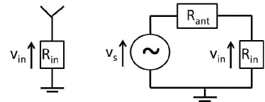
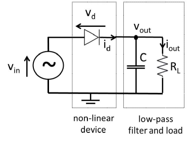
Figure 1: Antenna equivalent circuit (left) and a single diode rectifier (right).

III-B Rectifier and Diode Non-Linearity

A rectifier is always made of a non-linear device (e.g. diode) followed by a low pass filter (LPF) with load [3, 5, 6]. A simplified rectifier circuit is illustrated in Fig 1. We assume that its input impedance has been perfectly matched to the antenna impedance.

The current $i_{d}(t)$ flowing through an ideal diode (neglecting its series resistance) relates to the voltage drop across the diode $v_{d}(t)=v_{in}(t)-v_{out}(t)$ as $i_{d}(t)=i_{s}\big{(}e^{\frac{v_{d}(t)}{nv_{t}}}-1\big{)}$ where $i_{s}$ is the reverse bias saturation current, $v_{t}$ is the thermal voltage, $n$ is the ideality factor (assumed equal to $1.05$). In order to express the non-linearity of the diode, we take a Taylor expansion of the exponential function around a fixed operating voltage drop $v_{d}=a$ such that the diode current can be equivalently written as

$$i_{d}(t)=\sum_{i=0}^{\infty}k_{i}(v_{d}(t)-a)^{i}=\sum_{i=0}^{\infty}k_{i}(v_{in}(t)-v_{out}(t)-a)^{i},$$ (5)

where $k_{0}=i_{s}\big{(}e^{\frac{a}{nv_{t}}}-1\big{)}$ and $k_{i}=i_{s}\frac{e^{\frac{a}{nv_{t}}}}{i!\left(nv_{t}\right)^{i}}$, $i=1,\ldots,\infty$. The Taylor series expansion model is a small signal model that is valid only for the non-linear operation region of the diode. If the input voltage amplitude becomes large, the diode will be driven into the large signal operation region where the diode behaviour is dominated by the diode series resistance and the I-V relationship is linear [12].

As such, it is not easy to infer from (5) the exact dependencies of the diode current on the waveform parameters since both $v_{in}(t)$ and $v_{out}(t)$ will depend and fluctuate over time as a function of the waveform. Nevertheless, assuming a steady-state response, an ideal rectifier would deliver a constant (over time) output voltage $v_{out}$ whose level would depend on the peaks of the input voltage $v_{in}(t)$ [11]. As a consequence, the output current delivered to the load $i_{out}$ would also be constant. In this ideal rectifier, since $v_{out}$ is a constant (we drop the time dependency), a suitable choice of the operating voltage drop $a$ would be $a=\mathcal{E}\left\{v_{in}(t)-v_{out}\right\}=-v_{out}$ since $\mathcal{E}\left\{v_{in}(t)\right\}=\sqrt{R_{ant}}\mathcal{E}\left\{y(t)\right\}=0$. Under such assumptions, (5) can simply be written as

$$i_{d}(t)=\sum_{i=0}^{\infty}k_{i}v_{in}(t)^{i}=\sum_{i=0}^{\infty}k_{i}R_{ant}^{i/2}y(t)^{i},$$ (6)

which makes the dependency between the diode current $i_{d}(t)$, the received waveform $y(t)$ and therefore the transmitted waveforms $\left\{x_{m}(t)\right\}$ much more explicit.

The problem at hand will be the design of $\left\{x_{m}(t)\right\}$ such that the output DC current is maximized. Under the ideal rectifier assumption, the current delivered to the load in a steady-state response is constant and given by $i_{out}=\mathcal{E}\left\{i_{d}(t)\right\}$, i.e. the average over time of the current flowing through the diode. In order to make the optimization tractable, we truncate the Taylor expansion to the $n_{o}^{th}$ order. We consider two models: a non-linear model that truncates the Taylor expansion to the $n_{o}^{th}$ order but retains the fundamental non-linear behaviour of the diode and a linear model that truncates to the second order term and ignores the non-linearity.

III-C A Non-Linear Model

After truncation, the output DC current approximates as

$$i_{out}=\mathcal{E}\left\{i_{d}(t)\right\}\approx\sum_{i=0}^{n_{o}}k_{i}R_{ant}^{i/2}\mathcal{E}\left\{y(t)^{i}\right\}.$$ (7)

$$y(t)^{2} =\frac{1}{2}\sum_{n_{0},n_{1}}X_{n_{0}}X_{n_{1}}\left[\cos(w^{++}t+\delta^{++})+\cos(w^{+-}t+\delta^{+-})\right],$$ (8)

$$y(t)^{3} =\frac{1}{4}\sum_{n_{0},n_{1},n_{2}}X_{n_{0}}X_{n_{1}}X_{n_{2}}\left[\cos(w^{+++}t+\delta^{+++})+\cos(w^{++-}t+\delta^{++-})+\cos(w^{+-+}t+\delta^{+-+})+\cos(w^{+--}t+\delta^{+--})\right],$$ (9)

$$y(t)^{4} =\frac{1}{8}\sum_{\genfrac{}{}{0.0pt}{}{n_{0},n_{1},}{n_{2},n_{3}}}X_{n_{0}}X_{n_{1}}X_{n_{2}}X_{n_{3}}\left[\cos(w^{++++}t+\delta^{++++})+\cos(w^{++--}t+\delta^{++--})+\cos(w^{+++-}t+\delta^{+++-})+\cos(w^{++-+}t+\delta^{++-+})\right.$$

$$\hskip 56.9055pt\left.+\cos(w^{+-++}t+\delta^{+-++})+\cos(w^{+---}t+\delta^{+---})+\cos(w^{+-+-}t+\delta^{+-+-})+\cos(w^{+--+}t+\delta^{+--+})\right].$$ (10)

Applying (4) to (7) involves the computation of $y(t)^{i}$, illustrated in (8), (9) and (10) for $i=2,3,4$. In order to simplify the notations, (8) makes use of $w^{++}$ and $\delta^{++}$ to denote $w_{n_{0}}+w_{n_{1}}$ and $\delta_{n_{0}}+\delta_{n_{1}}$, respectively. Hence the sign of $\left\{w_{n_{0}},w_{n_{1}}\right\}$ and $\left\{\delta_{n_{0}},\delta_{n_{1}}\right\}$ is reflected as a superscript. Similarly, $w^{+-}=w_{n_{0}}-w_{n_{1}}$ and $\delta^{+-}=\delta_{n_{0}}-\delta_{n_{1}}$. In (9) and (10), we use the same convention, e.g. $w^{++++}=w_{n_{0}}+w_{n_{1}}+w_{n_{2}}+w_{n_{3}}$, $w^{++--}=w_{n_{0}}+w_{n_{1}}-w_{n_{2}}-w_{n_{3}}$, etc. Averaging over time, we get an approximation of the DC component of the current at the output of the rectifier (and the low-pass filter) with a multisine excitation over a multipath channel as

$$i_{out}\approx k_{0}+\sum_{i\hskip 2.84544pt\textnormal{even},i\geq 2}^{n_{o}}k_{i}R_{ant}^{i/2}\mathcal{E}\left\{y(t)^{i}\right\}$$ (11)

with $\mathcal{E}\left\{y(t)^{2}\right\}$, $\mathcal{E}\left\{y(t)^{4}\right\}$ and $\mathcal{E}\left\{y(t)^{6}\right\}$ detailed in (12), (14) and (16), respectively (at the top of next page). There is no odd (first, third, fifth, etc) order terms since $\mathcal{E}\left\{y(t)^{i}\right\}=\mathcal{E}\left\{y(t)^{i}\right\}=0$ for $i$ odd. In (8) and (10), only terms with an equal number of $+$ and $-$ lead to a DC component in (12) and (14) following the assumption on evenly spaced frequencies.

We note that the second order term (12) is linear, with the DC power being the sum of the power harvested on each frequency. On the other hand, even terms with $i\geq 4$ such as (14) and (16) are responsible for the non-linear behaviour of the diode since they are function of terms expressed as the product of contributions from different frequencies.

$$\mathcal{E}\left\{y(t)^{2}\right\} =\frac{1}{2}\left[\sum_{n=0}^{N-1}X_{n}^{2}\right]=\frac{1}{2}\left[\sum_{n=0}^{N-1}\left|\mathbf{h}_{n}\mathbf{w}_{n}\right|^{2}\right]=\frac{1}{2}\left[\sum_{n=0}^{N-1}\sum_{m_{0},m_{1}}s_{n,m_{0}}s_{n,m_{1}}A_{n,m_{0}}A_{n,m_{1}}\cos\left(\psi_{n,m_{0}}-\psi_{n,m_{1}}\right)\right],$$ (12)

$$\mathcal{E}\left\{y(t)^{4}\right\} =\frac{3}{8}\left[\sum_{\genfrac{}{}{0.0pt}{}{n_{0},n_{1},n_{2},n_{3}}{n_{0}+n_{1}=n_{2}+n_{3}}}X_{n_{0}}X_{n_{1}}X_{n_{2}}X_{n_{3}}\cos(\delta_{n_{0}}+\delta_{n_{1}}-\delta_{n_{2}}-\delta_{n_{3}})\right]=\frac{3}{8}\Re\left\{\sum_{\genfrac{}{}{0.0pt}{}{n_{0},n_{1},n_{2},n_{3}}{n_{0}+n_{1}=n_{2}+n_{3}}}\mathbf{h}_{n_{0}}\mathbf{w}_{n_{0}}\mathbf{h}_{n_{1}}\mathbf{w}_{n_{1}}\left(\mathbf{h}_{n_{2}}\mathbf{w}_{n_{2}}\right)^{*}\left(\mathbf{h}_{n_{3}}\mathbf{w}_{n_{3}}\right)^{*}\right\},$$ (13)

$$=\frac{3}{8}\left[\sum_{\genfrac{}{}{0.0pt}{}{n_{0},n_{1},n_{2},n_{3}}{n_{0}+n_{1}=n_{2}+n_{3}}}\sum_{\genfrac{}{}{0.0pt}{}{m_{0},m_{1},}{m_{2},m_{3}}}\Bigg{[}\prod_{j=0}^{3}s_{n_{j},m_{j}}A_{n_{j},m_{j}}\Bigg{]}\cos(\psi_{n_{0},m_{0}}+\psi_{n_{1},m_{1}}-\psi_{n_{2},m_{2}}-\psi_{n_{3},m_{3}})\right].$$ (14)

$$\mathcal{E}\left\{y(t)^{6}\right\} =\frac{5}{16}\Re\left\{\sum_{\genfrac{}{}{0.0pt}{}{n_{0},n_{1},n_{2},n_{3},n_{4},n_{5}}{n_{0}+n_{1}+n_{2}=n_{3}+n_{4}+n_{5}}}\mathbf{h}_{n_{0}}\mathbf{w}_{n_{0}}\mathbf{h}_{n_{1}}\mathbf{w}_{n_{1}}\mathbf{h}_{n_{2}}\mathbf{w}_{n_{2}}\left(\mathbf{h}_{n_{3}}\mathbf{w}_{n_{3}}\right)^{*}\left(\mathbf{h}_{n_{4}}\mathbf{w}_{n_{4}}\right)^{*}\left(\mathbf{h}_{n_{5}}\mathbf{w}_{n_{5}}\right)^{*}\right\},$$ (15)

$$=\frac{5}{16}\left[\sum_{\genfrac{}{}{0.0pt}{}{n_{0},n_{1},n_{2},n_{3},n_{4},n_{5}}{n_{0}+n_{1}+n_{2}=n_{3}+n_{4}+n_{5}}}\sum_{\genfrac{}{}{0.0pt}{}{m_{0},m_{1},m_{2},}{m_{3},m_{4},m_{5}}}\Bigg{[}\prod_{j=0}^{5}s_{n_{j},m_{j}}A_{n_{j},m_{j}}\Bigg{]}\cos(\psi_{n_{0},m_{0}}+\psi_{n_{1},m_{1}}+\psi_{n_{2},m_{2}}-\psi_{n_{3},m_{3}}-\psi_{n_{4},m_{4}}-\psi_{n_{5},m_{5}})\right].$$ (16)

III-D A Linear Model

The linear model was first introduced a few decades ago in [8] and recently became popular in the SWIPT literature [9]. It could be argued that if $y(t)$ is very small (i.e. for a very low input power), the high order ($>2$) terms would not contribute much to $i_{out}$. Hence, the linear model truncates the Taylor expansion to the second order $n_{o}=2$ such that $i_{out}\approx k_{0}+k_{2}R_{ant}\mathcal{E}\left\{y(t)^{2}\right\}$. It therefore completely omits the non-linearity behavior of the rectifier. The linear model is motivated by its simplicity rather than its accuracy. Its accuracy is actually questionable in the RF literature with experiments demonstrating that the non-linearity is an essential property of the rectenna and that a second order truncation of the Taylor expansion does not accurately model the rectification behavior of the diode [13]. Nevertheless, the loss incurred by using a linear vs a non-linear model in the WPT waveform and system design has never been addressed so far.

In the next section, we derive tools to design waveforms under the assumption of a linear and non-linear model.

IV WPT Waveform Optimization

Assuming the CSI (in the form of frequency response $h_{n,m}$) is known to the transmitter, we aim at finding the optimal set of amplitudes and phases $\mathbf{S},\mathbf{\Phi}$ that maximizes $i_{out}$, i.e.

$$\max_{\mathbf{S},\mathbf{\Phi}}\hskip 5.69046pti_{out}(\mathbf{S},\mathbf{\Phi})\hskip 8.5359pt\textnormal{subject to}\hskip 8.5359pt\frac{1}{2}\left\|\mathbf{S}\right\|_{F}^{2}\leq P.$$ (17)

From the previous section, we however note that the rectifier characteristics ${k_{i}}$ are functions of $a$. Since we chose $a=-v_{out}=-R_{L}i_{out}$ in the Taylor expansion, $k_{i}$ are therefore a function of the output DC current. Making this dependence explicit, we can write $i_{out}$ from (11) as

$$i_{out}\approx k_{0}\left(i_{out}\right)+\sum_{i\hskip 2.84544pt\textnormal{even},i\geq 2}^{n_{o}}k_{i}\left(i_{out}\right)R_{ant}^{i/2}\mathcal{E}\left\{y(t)^{i}\right\}.$$ (18)

Soving Problem (17) with $i_{out}$ given in (18) may seem challenging because of the occurence of $i_{out}$ on both sides of the equality in (18). Denoting $k_{0}^{\prime}=e^{\frac{a}{nv_{t}}}=e^{\frac{-R_{L}i_{out}}{nv_{t}}}$ and $k_{0}=i_{s}\left(k_{0}^{\prime}-1\right)$, we write (18) equivalently as

$$e^{\frac{R_{L}i_{out}}{nv_{t}}}\left(i_{out}+i_{s}\right)\approx i_{s}+\sum_{i\hskip 2.84544pt\textnormal{even},i\geq 2}^{n_{o}}\frac{k_{i}}{k_{0}^{\prime}}R_{ant}^{i/2}\mathcal{E}\left\{y(t)^{i}\right\}.$$ (19)

Interestingly, this leads to an expression where the r.h.s of (19) is independent of $a$ (and $i_{out}$) since $k_{i}/k_{0}^{\prime}=\frac{i_{s}}{i!\left(nv_{t}\right)^{i}}$, with $i$ even and $i\geq 2$. The l.h.s of (19) is on the other hand a monotonic increasing function of $i_{out}$. Hence the maximization of $i_{out}$ is equivalent to maximizing the r.h.s of (19), which is equivalent to maximizing the quantity

$$z_{DC}(\mathbf{S},\mathbf{\Phi})=\sum_{i\hskip 2.84544pt\textnormal{even},i\geq 2}^{n_{o}}k_{i}R_{ant}^{i/2}\mathcal{E}\left\{y(t)^{i}\right\}$$ (20)

since $i_{s}$ is a constant. In (20), we define $k_{i}=\frac{i_{s}}{i!\left(nv_{t}\right)^{i}}$ with a slight abuse of notation. Assuming $i_{s}=5\mu A$, a diode ideality factor $n=1.05$ and $v_{t}=25.86mV$, typical values of those parameters for second and fourth order are given by $k_{2}=0.0034$ and $k_{4}=0.3829$ (and will be used as such in any evaluation in the sequel). Hence, $\max_{\mathbf{S},\mathbf{\Phi}}i_{out}$ is equivalent to $\max_{\mathbf{S},\mathbf{\Phi}}z_{DC}$ and problem (17) can equivalently be written as

$$\max_{\mathbf{S},\mathbf{\Phi}}\hskip 5.69046ptz_{DC}(\mathbf{S},\mathbf{\Phi})\hskip 8.5359pt\textnormal{subject to}\hskip 8.5359pt\frac{1}{2}\left\|\mathbf{S}\right\|_{F}^{2}\leq P.$$ (21)

IV-A Linear Model-based Design

With the linear model, problem (21) is equivalent to

$$\max_{\mathbf{w}_{n}}\hskip 8.5359pt\sum_{n=0}^{N-1}\left|\mathbf{h}_{n}\mathbf{w}_{n}\right|^{2}\hskip 8.5359pt\textnormal{s.t.}\hskip 8.5359pt\frac{1}{2}\left[\sum_{n=0}^{N-1}\left\|\mathbf{w}_{n}\right\|^{2}\right]\leq P.$$ (22)

The solution simply consists in performing a matched beamformer on a single sinewave, namely the one corresponding to the strongest channel $\bar{n}=\arg\max_{i}\left\|\mathbf{h}_{i}\right\|^{2}$. Hence,

$$\mathbf{w}^{\star}_{n}=\left\{\begin{array}[]{l}\sqrt{2P}\>\mathbf{h}_{n}^{H}/\left\|\mathbf{h}_{n}\right\|,\hskip 5.69046ptn=\bar{n},\\ \mathbf{0},\hskip 5.69046ptn\neq\bar{n}.\end{array}\right.$$ (23)

We denote solution (23) as the adaptive single sinewave (ASS) strategy. With such a linear model, a single-sine waveform is favoured over a multisine waveform. Such a strategy has also appeared in the SWIPT literature with OFDM transmission, e.g. [14, 15].

Remark 1

For the extreme case where the channel is perfectly flat magnitude-wise, i.e. $\left\|\mathbf{h}_{n}\right\|=\left\|\mathbf{h}\right\|$ $\forall n$, ASS is not the only solution to problem (22). Allocating power uniformly over any non-empty subset $S$ of the $N$ sinewaves, i.e.

$$\mathbf{w}^{\star}_{n}=\left\{\begin{array}[]{l}\sqrt{\frac{2P}{\left|{S}\right|}}\>\mathbf{h}_{n}^{H}/\left\|\mathbf{h}\right\|,\hskip 5.69046ptn\in S,\\ \mathbf{0},\hskip 5.69046ptn\notin S,\end{array}\right.$$ (24)

leads to the same objective value. If the channel is not perfectly flat, ASS would be the unique solution to problem (22).

IV-B Towards a Non-Linear Model-based Design

To get some insights into the necessity to account for the non-linear terms (e.g. $4^{th}$,$6^{th}$) and into the impact of multipath on the waveform design, let us consider a toy example with the simplest multisine: $N=2$, $M=1$. We also assume $n_{o}=4$. For readibility, we drop the antenna index and assume real frequency domain channel $h_{n}$. Since $\bar{\psi}_{n}=0$, let us choose $\phi_{n}=0$ so that $\psi_{n}=0$ (and all $\cos(.)=1$) in (12) and (14) $\forall n,m$. Since for $N=2$, indices $n_{0}$, $n_{1}$, $n_{2}$, $n_{3}$ in (14) can take either value 0 or 1, we can easily identify cases for which $n_{0}+n_{1}=n_{2}+n_{3}$ and then write from (20)

$$z_{DC}(s_{0},s_{1})=\tilde{k}_{2}\left(s_{0}^{2}A_{0}^{2}+s_{1}^{2}A_{1}^{2}\right)\\ +\tilde{k}_{4}\left[\left(s_{0}^{2}A_{0}^{2}+s_{1}^{2}A_{1}^{2}\right)^{2}+2s_{0}^{2}s_{1}^{2}A_{0}^{2}A_{1}^{2}\right]$$ (25)

where $\tilde{k}_{2}=k_{2}R_{ant}/2$ and $\tilde{k}_{4}=3k_{4}R_{ant}^{2}/8$. From (25), we note that $z_{DC}(s_{0},s_{1})$ is a function of the term $s_{0}^{2}A_{0}^{2}+s_{1}^{2}A_{1}^{2}$, whose maximization subject to the sum power constraint $s_{0}^{2}+s_{1}^{2}\leq 2P$ would lead to the ASS strategy (23), i.e. allocate all the power to sinewave 1 if $A_{1}>A_{0}$ and to sinewave 0 otherwise. However the presence of the term $2s_{0}^{2}s_{1}^{2}A_{0}^{2}A_{1}^{2}$ suggests that such a single-sinewave strategy is in general sub-optimal for the maximization of $z_{DC}$. In problem (21) with $N=2$ and $M=1$, we note that equality $\frac{1}{2}\left\|\mathbf{S}\right\|_{F}^{2}=P$ is satisfied at optimality and we write the Lagrangian as

$$\mathcal{L}=\tilde{k}_{2}\left(s_{0}^{2}A_{0}^{2}+s_{1}^{2}A_{1}^{2}\right)+\tilde{k}_{4}\left(s_{0}^{4}A_{0}^{4}+s_{1}^{4}A_{1}^{4}+4s_{0}^{2}s_{1}^{2}A_{0}^{2}A_{1}^{2}\right)\\ +\lambda\left(s_{0}^{2}+s_{1}^{2}-2P\right).$$ (26)

Differentiating w.r.t. $s_{0}$, $s_{1}$, $\lambda$ and equating to 0, we find three valid stationary points $(s_{0}^{2},s_{1}^{2})$ (such that $0\leq s_{0}^{2}\leq 2P$ and $0\leq s_{1}^{2}\leq 2P$) given by $(2P,0)$, $(0,2P)$ and $(s_{0}^{\star 2},s_{1}^{\star 2})$ where

$$s_{0}^{\star 2} =\frac{8P\tilde{k}_{4}A_{0}^{2}A_{1}^{2}+\tilde{k}_{2}A_{0}^{2}-4P\tilde{k}_{4}A_{1}^{4}-\tilde{k}_{2}A_{1}^{2}}{8\tilde{k}_{4}A_{0}^{2}A_{1}^{2}-2\tilde{k}_{4}A_{0}^{4}-2\tilde{k}_{4}A_{1}^{4}},$$ (27)

$$s_{1}^{\star 2} =2P-s_{0}^{\star 2}.$$ (28)

For given $A_{0}$, $A_{1}$, the global optimum strategy is given by one of those three stationary points. The maximum achievable $z_{DC}^{\star}=\max\big{\{}z_{DC}(\sqrt{2P},0),z_{DC}(0,\sqrt{2P}),z_{DC}(s_{0}^{\star},s_{1}^{\star})\big{\}}$. The first two points correspond to the ASS strategy, allocating transmit power to sinewave 0 and 1, respectively. Fig 2 illustrates $z_{DC}$ as a function of $A_{1}$ for $A_{0}=1$ with three strategies: single-sinewave transmission (i.e. $s_{0}=0$ and $s_{1}=0$) and the optimal transmission leading to $z_{DC}^{\star}$. The contours of $z_{DC}$ as a function of $s_{0}^{2}$ and $s_{1}^{2}$ are also illustrated for $A_{0}=1$ and $A_{1}=0.75,1,1.15$. We note that the ASS strategy is optimal if $A_{0}$ is sufficiently larger than $A_{1}$ or inversely. However, when the channel is frequency flat, i.e. $A_{1}\approx A_{0}$, the optimal strategy would allocate power to the two sinewaves and the ASS strategy is suboptimal.

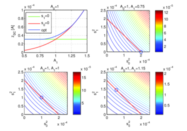
Figure 2: $z_{DC}$ as a function of $A_{1}$ and contours of $z_{DC}$ as a function of $s_{0}^{2}$ and $s_{1}^{2}$. The straight line refers to the power constraint and the circle to the optimal power allocation strategy. $P=-40dBW$.

The results, though based on a very simple scenario, highlight that depending on the CSI, the transmission waveform should be adapted if we aim at maximizing the output DC power. Moreover, it also shows the benefits of allocating power over multiple sinewaves for some channel states, which is in sharp contrast with the ASS strategy (23) originating from the linear model. More generally, looking at (14), the ASS strategy would unlikely be a right strategy if we account for the non-linearity of the diode, due to the presence of $\prod_{j=0}^{3}s_{n_{j},m_{j}}A_{n_{j},m_{j}}$ in the fourth order term.

Remark 2

It should be noted that RF experiments in [5, 6, 7] have shown the benefits of allocating power uniformly across multiple sinewaves. The above discussion highlights theoretically the benefits of allocating power over multiple sinewaves for some channel states and therefore backs up the experimental results. On the other hand, the linear model motivates the use of a single sinewave (ASS) for all channel states, and therefore contradicts the RF experiment results.

Deriving a formal algorithm that can generate optimized waveforms for any multipath configuration and any $N$, $M$, $n_{o}$ so as to maximize the DC output current is a non-trivial problem that is discussed in the next section.

IV-C Non-Linear Model-based Design

We aim at deriving a waveform design strategy that is general enough to cope with any Taylor expansion order $n_{o}$. The optimal phases $\mathbf{\Phi}$ can be obtained first in closed form and the optimal amplitudes $\mathbf{S}$ can then be computed numerically.

To maximize $z_{DC}(\mathbf{S},\mathbf{\Phi})$, we should guaranteee all $\cos(.)$ to be equal to 1 in (12), (14) and (16). This can be satisfied by choosing $\psi_{n,m}=0$ $\forall n,m$ (and therefore $\delta_{n}=0$ $\forall n$), which implies from (3) to choose the optimal sinewave phases as

$$\phi_{n,m}^{\star}=-\bar{\psi}_{n,m}.$$ (29)

$\mathbf{\Phi}^{\star}$ is obtained by collecting $\phi_{n,m}^{\star}$ $\forall n,m$ into matrix. With such a phase choice, all sinewaves in (4) are in-phase at the rectenna input. Moreover, $\psi_{n,m}=0$ and $X_{n}=\sum_{m=1}^{M}s_{n,m}A_{n,m}$ such that $z_{DC}(\mathbf{S},\mathbf{\Phi}^{\star})$ is simply obtained from (20) with all $\cos(.)$ replaced by 1 in (12), (14) and (16).

Recall from [17] that a monomial is defined as the function $g:\mathbb{R}_{++}^{N}\rightarrow\mathbb{R}:g(\mathbf{x})=cx_{1}^{a_{1}}x_{2}^{a_{2}}\ldots x_{N}^{a_{N}}$ where $c>0$ and $a_{i}\in\mathbb{R}$. A sum of $K$ monomials is called a posynomial and can be written as $f(\mathbf{x})=\sum_{k=1}^{K}g_{k}(\mathbf{x})$ with $g_{k}(\mathbf{x})=c_{k}x_{1}^{a_{1k}}x_{2}^{a_{2k}}\ldots x_{N}^{a_{Nk}}$ where $c_{k}>0$. As we can see from (12), (14) and (16), $z_{DC}(\mathbf{S},\mathbf{\Phi}^{\star})$ is a posynomial, and so it is for any order $n_{o}$ in the Taylor expansion. The higher the order, the larger the number of terms in the posynomial.

The optimization problem becomes $\max_{\mathbf{S}}z_{DC}(\mathbf{S},\mathbf{\Phi}^{\star})$ subject to $\frac{1}{2}\left\|\mathbf{S}\right\|_{F}^{2}\leq P$. It therefore consists in maximizing a posynomial subject to a power constraint (which itself is written as a posynomial). This problem is not a standard Geometric Program (GP) but it can be transformed to an equivalent problem by introducing an auxiliary variable $t_{0}$

$$\min_{\mathbf{S},t_{0}}\hskip 8.5359pt 1/t_{0}$$ (30)

subject to $$\frac{1}{2}\left\|\mathbf{S}\right\|_{F}^{2}\leq P,$$ (31)

$$z_{DC}(\mathbf{S},\mathbf{\Phi}^{\star})/t_{0}\geq 1.$$ (32)

This is known as a Reverse Geometric Program due to the minimization of a posynomial subject to upper and lower bounds inequality constraints [18, 17]. Note that $z_{DC}(\mathbf{S},\mathbf{\Phi}^{\star})/t_{0}\geq 1$ is equivalent to $t_{0}/z_{DC}(\mathbf{S},\mathbf{\Phi}^{\star})\leq 1$. However $1/z_{DC}(\mathbf{S},\mathbf{\Phi}^{\star})$ is not a posynomial, therefore preventing the use of standard GP tools. The idea is to lower bound $z_{DC}(\mathbf{S},\mathbf{\Phi}^{\star})$ by a monomial $\bar{z}_{DC}(\mathbf{S})$, i.e. upper bound $1/z_{DC}(\mathbf{S},\mathbf{\Phi}^{\star})$ by the monomial $1/\bar{z}_{DC}(\mathbf{S})$ (since the inverse of a monomial is still a monomial) [18]. Let $\left\{g_{k}(\mathbf{S},\mathbf{\Phi}^{\star})\right\}$ be the monomial terms in the posynomial $z_{DC}(\mathbf{S},\mathbf{\Phi}^{\star})=\sum_{k=1}^{K}g_{k}(\mathbf{S},\mathbf{\Phi}^{\star})$. The choice of the lower bound relies on the fact that an arithmetic mean (AM) is greater or equal to the geometric mean (GM). Hence, $z_{DC}(\mathbf{S},\mathbf{\Phi}^{\star})\geq\prod_{k=1}^{K}\left(\frac{g_{k}(\mathbf{S},\mathbf{\Phi}^{\star})}{\gamma_{k}}\right)^{\gamma_{k}}=\bar{z}_{DC}(\mathbf{S})$, where $\gamma_{k}\geq 0$ and $\sum_{k=1}^{K}\gamma_{k}=1$. Since

$$1/z_{DC}(\mathbf{S},\mathbf{\Phi}^{\star})\leq 1/\bar{z}_{DC}(\mathbf{S}),$$ (33)

we can replace (in a conservative way) inequality $t_{0}/z_{DC}(\mathbf{S},\mathbf{\Phi}^{\star})\leq 1$ by $t_{0}/\bar{z}_{DC}(\mathbf{S})=t_{0}\prod_{k=1}^{K}\left(g_{k}(\mathbf{S},\mathbf{\Phi}^{\star})/\gamma_{k}\right)^{-\gamma_{k}}\leq 1$. For a given choice of $\left\{\gamma_{k}\right\}$, problem (30)-(32) is now replaced by the standard GP

$$\min_{\mathbf{S},t_{0}}\hskip 8.5359pt 1/t_{0}$$ (34)

subject to $$\frac{1}{2}\left\|\mathbf{S}\right\|_{F}^{2}\leq P,$$ (35)

$$t_{0}\prod_{k=1}^{K}\left(\frac{g_{k}(\mathbf{S},\mathbf{\Phi}^{\star})}{\gamma_{k}}\right)^{-\gamma_{k}}\leq 1,$$ (36)

that can be solved using existing software, e.g. CVX [20].

Note that the tightness of the upper bound (33) heavily depends on the choice of $\left\{\gamma_{k}\right\}$. Following [19, 17], an iterative procedure can be used to tighten the bound, where at each iteration the standard GP (34)-(36) is solved for an updated set of $\left\{\gamma_{k}\right\}$. Assuming a feasible set of magnitude $\mathbf{S}^{(i-1)}$ at iteration $i-1$, compute at iteration $i$ $\gamma_{k}=g_{k}(\mathbf{S}^{(i-1)},\mathbf{\Phi}^{\star})/z_{DC}(\mathbf{S}^{(i-1)},\mathbf{\Phi}^{\star})$ $\forall k$ and solve problem (34)-(36) to obtain $\mathbf{S}^{(i)}$. Repeat the iterations till convergence. Algorithm 1 summarizes the procedure.

Algorithm 1 WPT Waveform

1:Initialize: $i\leftarrow 0$, $\mathbf{\Phi}^{\star}$ in (29), $\mathbf{S}$, $z_{DC}^{(0)}=0$

2:repeat

3:     $i\leftarrow i+1$, $\ddot{\mathbf{S}}\leftarrow\mathbf{S}$

4:     $\gamma_{k}\leftarrow g_{k}(\ddot{\mathbf{S}},\mathbf{\Phi}^{\star})/z_{DC}(\ddot{\mathbf{S}},\mathbf{\Phi}^{\star})$, $k=1,\ldots,K$

5:     $\mathbf{S}\leftarrow\arg\min\eqref{standard_GP}-\eqref{standard_GP_constraint_2}$

6:     $z_{DC}^{(i)}\leftarrow z_{DC}(\mathbf{S},\mathbf{\Phi}^{\star})$

7:until $\left|z_{DC}^{(i)}-z_{DC}^{(i-1)}\right|<\epsilon$ or $i=i_{\max}$

Note that the successive approximation method used in the Algorithm 1 is also known as a sequential convex optimization or inner approximation method [21]. It cannot guarantee to converge to the global solution of the original problem, but only to yield a point fulfilling the KKT conditions [21, 22]. However, it has been shown in [17] by simulation that such an iterative algorithm often converges to the global optimum.

Remark 3

Non-linearity is obviously meaningful only for $N\geq 2$. For $N=1$, both linear and non-linear designs boil down to the simple matched beamformer $\mathbf{w}=\sqrt{2P}\mathbf{h}^{H}/\left\|\mathbf{h}\right\|$.

IV-D Decoupling Space and Frequency Domains

When $M>1$, previous section derives a general methodology to design waveform weights jointly across space and frequency. It is worth wondering whether we can decouple the design of the spatial and frequency domain weights without impacting performance. The optimal phases in (29) are those of a matched beamformer. Looking at (12), (13) and (15), the optimum weight vector $\mathbf{w}_{n}$ that maximizes the $2^{nd}$, $4^{th}$ and $6^{th}$ order terms is actually a matched beamformer of the form

$$\mathbf{w}_{n}=s_{n}\mathbf{h}_{n}^{H}/\left\|\mathbf{h}_{n}\right\|$$ (37)

such that, from (4), $y(t)=\sum_{n=0}^{N-1}\left\|\mathbf{h}_{n}\right\|s_{n}\cos\left(w_{n}t\right)=\Re\left\{\sum_{n=0}^{N-1}\left\|\mathbf{h}_{n}\right\|s_{n}e^{jw_{n}t}\right\}$. Hence, with (37), the multi-antenna multi-sine WPT weight optimization is converted into an effective single antenna multi-sine WPT optimization with the effective channel gain on frequency $n$ given by $\left\|\mathbf{h}_{n}\right\|$ and the amplitude of the $n^{th}$ sinewave given by $s_{n}$ (subject to $\sum_{n=0}^{N-1}s_{n}^{2}=2P$). The optimum magnitude $s_{n}$ in (37) can now be obtained by using the posynomial maximization methodology of Section IV-C. Namely, plugging (37) into (12), (13) and (15), we get (38).

$$\mathcal{E}\left\{y(t)^{2}\right\}=\frac{1}{2}\left[\sum_{n=0}^{N-1}\left\|\mathbf{h}_{n}\right\|^{2}s_{n}^{2}\right],\mathcal{E}\left\{y(t)^{4}\right\}=\frac{3}{8}\left[\sum_{\genfrac{}{}{0.0pt}{}{n_{0},n_{1},n_{2},n_{3}}{n_{0}+n_{1}=n_{2}+n_{3}}}\Bigg{[}\prod_{j=0}^{3}s_{n_{j}}\left\|\mathbf{h}_{n_{j}}\right\|\Bigg{]}\right],\mathcal{E}\left\{y(t)^{6}\right\}=\frac{5}{16}\left[\sum_{\genfrac{}{}{0.0pt}{}{n_{0},n_{1},n_{2},n_{3},n_{4},n_{5}}{n_{0}+n_{1}+n_{2}=n_{3}+n_{4}+n_{5}}}\Bigg{[}\prod_{j=0}^{5}s_{n_{j}}\left\|\mathbf{h}_{n_{j}}\right\|\Bigg{]}\right]$$ (38)

$z_{DC}\left(\mathbf{s}\right)=\sum_{i\hskip 2.84544pt\textnormal{even},i\geq 2}^{n_{o}}k_{i}R_{ant}^{i/2}\mathcal{E}\left\{y(t)^{i}\right\}$ is now only a function of the $N$-dimensional vector $\mathbf{s}=\left[\begin{array}[]{c}s_{0},\ldots,s_{N-1}\end{array}\right]$. Following the posynomial maximization methodology, we can write $z_{DC}(\mathbf{s})=\sum_{k=1}^{K}g_{k}(\mathbf{s})$, apply the AM-GM inequality and write the standard GP problem

$$\min_{\mathbf{s},t_{0}}\hskip 8.5359pt 1/t_{0}$$ (39)

subject to $$\frac{1}{2}\left\|\mathbf{s}\right\|^{2}\leq P,$$ (40)

$$t_{0}\prod_{k=1}^{K}\left(\frac{g_{k}(\mathbf{s})}{\gamma_{k}}\right)^{-\gamma_{k}}\leq 1.$$ (41)

Algorithm 2 summarizes the design methodology with spatial and frequency domain decoupling.

Algorithm 2 WPT Waveform with Decoupling

1:Initialize: $i\leftarrow 0$, $\mathbf{w}_{n}$ in (37), $\mathbf{s}$, $z_{DC}^{(0)}=0$

2:repeat

3:     $i\leftarrow i+1$, $\ddot{\mathbf{s}}\leftarrow\mathbf{s}$

4:     $\gamma_{k}\leftarrow g_{k}(\ddot{\mathbf{s}})/z_{DC}(\ddot{\mathbf{s}})$, $k=1,\ldots,K$

5:     $\mathbf{s}\leftarrow\arg\min\eqref{standard_GP_simple}-\eqref{standard_GP_constraint_2_simple}$

6:     $z_{DC}^{(i)}\leftarrow z_{DC}(\mathbf{s})$

7:until $\left|z_{DC}^{(i)}-z_{DC}^{(i-1)}\right|<\epsilon$ or $i=i_{\max}$

Such an approach would lead to the same performance as the joint space-frequency design of Algorithm 1 but would significantly reduce the computational complexity since only a $N$-dimensional vector $\mathbf{s}$ is to be optimized numerically, compared to the $N\times M$ matrix $\mathbf{S}$ of Algorithm 1.

IV-E PAPR Constraints

In practice, it may be useful to constrain the PAPR of the transmitted waveform in order to increase the efficiency of the power amplifier. From (1), the PAPR on antenna $m$ can be defined as $PAPR_{m}=\frac{\max_{t}\left|x_{m}(t)\right|^{2}}{\mathcal{E}\small\{|x_{m}(t)|^{2}\small\}}=\frac{\max_{t}\left|x_{m}(t)\right|^{2}}{\frac{1}{2}\left\|\mathbf{s}_{m}\right\|^{2}}$. The PAPR constraint on antenna $m$ writes as $PAPR_{m}\leq\eta$. Problem (17) is now subject to an extra constraint

$$\max_{\mathbf{S},\mathbf{\Phi}}\hskip 8.5359pt i_{out}(\mathbf{S},\mathbf{\Phi})$$ (42)

subject to $$\frac{1}{2}\left\|\mathbf{S}\right\|_{F}^{2}\leq P,$$ (43)

$$PAPR_{m}\leq\eta,\forall m.$$ (44)

In the sequel, we will assume the use of the phase $\mathbf{\Phi}^{\star}$ in (29) and optimize the amplitude $\mathbf{S}$.

By oversampling the transmit signals at $t_{q}=q\frac{T}{NO_{s}}$ for $q=0,\ldots,NO_{s}-1$ with $T=1/\Delta_{f}=\frac{2\pi}{\Delta_{w}}$ and $O_{s}$ the oversampling factor, the PAPR constraint can be rewritten as $\left|x_{m}(t_{q})\right|^{2}\leq\frac{1}{2}\eta\left\|\mathbf{s}_{m}\right\|^{2}$, $\forall q=0,\ldots,NO_{s}-1$ for sufficiently large $O_{s}$. Assuming the phase $\mathbf{\Phi}^{\star}$ in (29), we can write

$$\left|x_{m}(t_{q})\right|^{2}=\sum_{n_{0},n_{1}}s_{n_{0},m}s_{n_{1},m}\\ \cos\left(w_{n_{0}}t_{q}+\phi^{\star}_{n_{0},m}\right)\cos\left(w_{n_{1}}t_{q}+\phi^{\star}_{n_{1},m}\right).$$ (45)

The quantity $\left|x_{m}(t_{q})\right|^{2}$ is not a posynomial anymore as some of the coefficients $c_{k}$ are negative. $\left|x_{m}(t_{q})\right|^{2}$ is now written as a signomial, i.e. the sum of monomials whose coefficients $c_{k}$ can be either positive or negative, $f(\mathbf{x})=f_{1}(\mathbf{x})-f_{2}(\mathbf{x})$ where $f_{j}(\mathbf{x})=\sum_{k=1}^{K_{j}}g_{jk}(\mathbf{x})$ and $g_{jk}(\mathbf{x})=c_{jk}x_{1}^{a_{1jk}}x_{2}^{a_{2jk}}\ldots x_{N}^{a_{Njk}}$ with $c_{jk}>0$. Let us write the signomial $\left|x_{m}(t_{q})\right|^{2}=f_{mq}(\mathbf{S},\mathbf{\Phi}^{\star})=f_{mq1}(\mathbf{S},\mathbf{\Phi}^{\star})-f_{mq2}(\mathbf{S},\mathbf{\Phi}^{\star})$. We therefore have the inequality $f_{mq1}(\mathbf{S},\mathbf{\Phi}^{\star})-f_{mq2}(\mathbf{S},\mathbf{\Phi}^{\star})\leq\frac{1}{2}\eta\left\|\mathbf{s}_{m}\right\|^{2}$ or equivalently $\frac{f_{mq1}(\mathbf{S},\mathbf{\Phi}^{\star})}{\frac{1}{2}\eta\left\|\mathbf{s}_{m}\right\|^{2}+f_{mq2}(\mathbf{S},\mathbf{\Phi}^{\star})}\leq 1$. This is a standard sign inequality but the quotient of posynomials is not a posynomial. Writing the denominator as a sum of monomials, $\frac{1}{2}\eta\left\|\mathbf{s}_{m}\right\|^{2}+f_{mq2}(\mathbf{S},\mathbf{\Phi}^{\star})=\sum_{k=1}^{K_{mq2}}g_{mq2k}(\mathbf{S},\mathbf{\Phi}^{\star})$, we can perform a single condensation and replace the original inequality by the following inequality

$$f_{mq1}(\mathbf{S},\mathbf{\Phi}^{\star})\prod_{k=1}^{K_{mq2}}\left(\frac{g_{mq2k}(\mathbf{S},\mathbf{\Phi}^{\star})}{\gamma_{mq2k}}\right)^{-\gamma_{mq2k}}\leq 1$$ (46)

with $\gamma_{mq2k}\geq 0$ and $\sum_{k=1}^{K_{mq2}}\gamma_{mq2k}=1$. For a given choice of $\left\{\gamma_{k},\gamma_{mq2k}\right\}$ and assuming $\mathbf{\Phi}^{\star}$, the optimization problem (42)-(44) is now replaced by the standard GP

$$\min_{\mathbf{S},t_{0}}\hskip 8.5359pt 1/t_{0}$$ (47)

s.t. $$\frac{1}{2}\left\|\mathbf{S}\right\|_{F}^{2}\leq P,$$ (48)

$$t_{0}\prod_{k=1}^{K}\left(\frac{g_{k}(\mathbf{S},\mathbf{\Phi}^{\star})}{\gamma_{k}}\right)^{-\gamma_{k}}\leq 1,$$ (49)

$$f_{mq1}(\mathbf{S},\mathbf{\Phi}^{\star})\prod_{k=1}^{K_{mq2}}\left(\frac{g_{mq2k}}{\gamma_{mq2k}}\right)^{-\gamma_{mq2k}}\leq 1,\forall m,q$$ (50)

Problem (47)-(50) can now be solved at each iteration of an iterative procedure where $\left\{\gamma_{k},\gamma_{mq2k}\right\}$ are updated. The whole optimization procedure is summarized in Algorithm 3.

Algorithm 3 WPT Waveform with PAPR Constraints

1:Initialize: $i\leftarrow 0$, $\mathbf{\Phi}^{\star}$ in (29), $\mathbf{S}$, $z_{DC}^{(0)}=0$

2:repeat

3:     $i\leftarrow i+1$, $\ddot{\mathbf{S}}\leftarrow\mathbf{S}$

4:     $\gamma_{k}\leftarrow g_{k}(\ddot{\mathbf{S}},\mathbf{\Phi}^{\star})/z_{DC}(\ddot{\mathbf{S}},\mathbf{\Phi}^{\star})$, $k=1,\ldots,K$

5:     $\gamma_{mq2k}\leftarrow g_{mq2k}(\ddot{\mathbf{S}},\mathbf{\Phi}^{\star})/\big{(}\frac{1}{2}\eta\left\|\ddot{\mathbf{s}}_{m}\right\|^{2}+f_{mq2}(\ddot{\mathbf{S}},\mathbf{\Phi}^{\star})\big{)}$, $m=1,\ldots,M$, $q=0,\ldots,NO_{s}-1$, $k=1,\ldots,K_{mq2}$

6:     $\mathbf{S}\leftarrow\arg\min\eqref{standard_GP_PAPR}-\eqref{standard_GP_PAPR_3}$

7:     $z_{DC}^{(i)}\leftarrow z_{DC}(\mathbf{S},\mathbf{\Phi}^{\star})$

8:until $\left|z_{DC}^{(i)}-z_{DC}^{(i-1)}\right|<\epsilon$ or $i=i_{\max}$

Note that for $M>1$, decoupling the space and frequency domains (similarly to Section IV-D) would lead to a suboptimal design compared to the joint space-frequency design of Algorithm 3 in the presence of PAPR constraints.

IV-F Multiple Rectennas

Consider now the extension to $U$ rectennas. Those rectennas could either belong to a single user (i.e. point-to-point MIMO WPT) or spread across multiple users (i.e. MU-MISO WPT). In this multiple rectenna setup, the energy harvested by a given rectenna $z_{DC,q}$ in general depends on the energy harvested by the other rectennas $z_{DC,p}$, $p\neq q$. Indeed, a given waveform may be suitable for a given rectenna but found inefficient for another rectenna. Hence, there exists a trade-off between the energy harvested by the different rectennas. The energy region $\mathcal{Z}_{DC}$ formulates this trade-off by expressing the set of all rectenna harvested energy $\left(z_{DC,1},\ldots,z_{DC,U}\right)$ that are simultaneously achievable. The boundary of the energy region can be derived by considering a weighted sum of DC component at each user where weights $v_{u}$, $u=1,\ldots,U$, account for the multi-rectenna fairness.

The optimization problem now consists in finding the optimal set of amplitudes and phases (across frequencies) that maximizes the weighted sum of DC components $z_{DC,u}$, i.e.

$$\max_{\mathbf{S},\mathbf{\Phi}}Z_{DC}(\mathbf{S},\mathbf{\Phi})=\sum_{u=1}^{U}v_{u}z_{DC,u}(\mathbf{S},\mathbf{\Phi})\hskip 5.69046pt\textnormal{s.t.}\hskip 5.69046pt\frac{1}{2}\left\|\mathbf{S}\right\|_{F}^{2}\leq P.$$ (51)

From Section II, after adding the index $u$ to any user specific variable, we define $X_{n,u}e^{j\delta_{n,u}}=\sum_{m=1}^{M}s_{n,m}A_{n,m,u}e^{j\psi_{n,m,u}}$ and $A_{n,m,u}e^{j\psi_{n,m,u}}=e^{j\phi_{n,m}}h_{n,m,u}$ with $h_{n,m,u}=A_{n,m,u}e^{j\bar{\psi}_{n,m,u}}$ the frequency response of the channel of rectenna $u$ on transmit antenna $m$ at $w_{n}$.

IV-F1 Linear Model

The ASS strategy (23) is generalized as

$$\max_{\mathbf{w}_{n}}\hskip 8.5359pt\sum_{n=0}^{N-1}\big{\|}\tilde{\mathbf{H}}_{n}\mathbf{w}_{n}\big{\|}^{2}\hskip 8.5359pt\textnormal{s.t.}\hskip 8.5359pt\frac{1}{2}\left[\sum_{n=0}^{N-1}\left\|\mathbf{w}_{n}\right\|^{2}\right]\leq P$$ (52)

with $\tilde{\mathbf{H}}_{n}=\big{[}\begin{array}[]{ccc}\tilde{\mathbf{h}}_{n,1}^{T}&\ldots&\tilde{\mathbf{h}}_{n,U}^{T}\end{array}\big{]}^{T}$ and $\tilde{\mathbf{h}}_{n,u}=\sqrt{k_{2}v_{u}}\mathbf{h}_{n,u}$. The solution consists in transmitting on a single sinewave $\bar{n}=\arg\max_{i}\lambda_{max}\big{(}\tilde{\mathbf{H}}_{i}^{H}\tilde{\mathbf{H}}_{i}\big{)}$ and along the dominant right singular vector of $\tilde{\mathbf{H}}_{\bar{n}}$. Hence,

$$\mathbf{w}^{\star}_{n}=\left\{\begin{array}[]{l}\sqrt{2P}\>\mathbf{v}_{max,n},\hskip 5.69046ptn=\bar{n},\\ \mathbf{0},\hskip 5.69046ptn\neq\bar{n},\end{array}\right.$$ (53)

where $\mathbf{v}_{max,n}$ is the dominant right singular vector of $\tilde{\mathbf{H}}_{n}$. Solution (53) naturally boils down to (23) for $U=1$.

IV-F2 Non-Linear Model

Unfortunately, guaranteeing $\psi_{n,m,u}=0$ $\forall n,m,u$ is not possible ($NMU$ constraints and $NM$ variables only). Hence, for a given choice of phase matrix $\mathbf{\Phi}=\mathbf{\Phi}^{\prime}$, some cosine functions in (12), (14) and (16) are positive while others are negative. $Z_{DC}(\mathbf{S},\mathbf{\Phi}^{\prime})$ is now a signomial since some of the coefficients $c_{k}$ are negative.

Similarly to the single rectenna scenario, we can convert the maximization problem into a minimization by introducing the auxiliary variable $t_{0}$. The problem writes as (30)-(32) with (32) replaced by $Z_{DC}(\mathbf{S},\mathbf{\Phi}^{\prime})/t_{0}\geq 1$. Condition $Z_{DC}(\mathbf{S},\mathbf{\Phi}^{\prime})=f_{1}(\mathbf{S},\mathbf{\Phi}^{\prime})-f_{2}(\mathbf{S},\mathbf{\Phi}^{\prime})\geq t_{0}$ can be replaced by

$$\frac{t_{0}+f_{2}(\mathbf{S},\mathbf{\Phi}^{\prime})}{\bar{f}_{1}(\mathbf{S},\mathbf{\Phi}^{\prime})}=\left(t_{0}+f_{2}(\mathbf{S},\mathbf{\Phi}^{\prime})\right)\prod_{k=1}^{K_{1}}\left(\frac{g_{1k}}{\gamma_{1k}}\right)^{-\gamma_{1k}}\leq 1$$ (54)

where $\gamma_{1k}\geq 0$, $\sum_{k=1}^{K_{1}}\gamma_{1k}=1$ and $\left\{g_{1k}\right\}$ are the monomial terms in the posynomial $f_{1}(\mathbf{S},\mathbf{\Phi}^{\prime})=\sum_{k=1}^{K_{1}}g_{1k}(\mathbf{S},\mathbf{\Phi}^{\prime})$. For a given choice of $\left\{\gamma_{1k}\right\}$, we now get the standard GP

$$\min_{\mathbf{S},t_{0}}\hskip 8.5359pt 1/t_{0}$$ (55)

s.t. $$\frac{1}{2}\left\|\mathbf{S}\right\|_{F}^{2}\leq P,$$ (56)

$$\left(t_{0}+f_{2}(\mathbf{S},\mathbf{\Phi}^{\prime})\right)\prod_{k=1}^{K_{1}}\left(\frac{g_{1k}(\mathbf{S},\mathbf{\Phi}^{\prime})}{\gamma_{1k}}\right)^{-\gamma_{1k}}\leq 1.$$ (57)

Similarly to the single rectenna optimization, Problem (55)-(57) can now be solved at each iteration of an iterative procedure where $\left\{\gamma_{1k}\right\}$ are updated. Note that Problem (55)-(57) boils down to Problem (34)-(36) if $f_{2}=0$. The whole optimization procedure is summarized in Algorithm 4.

Algorithm 4 WPT Waveform with Multiple Rectennas

1:Initialize: $i\leftarrow 0$, $\mathbf{\Phi}^{\prime}$, $\mathbf{S}$, $Z_{DC}^{(0)}=0$

2:repeat

3:     $i\leftarrow i+1$, $\ddot{\mathbf{S}}\leftarrow\mathbf{S}$

4:     $\gamma_{1k}\leftarrow g_{1k}(\ddot{\mathbf{S}},\mathbf{\Phi}^{\prime})/f_{1}(\ddot{\mathbf{S}},\mathbf{\Phi}^{\prime})$, $k=1,\ldots,K_{1}$

5:     $\mathbf{S}\leftarrow\arg\min\eqref{standard_GP_MU_2}-\eqref{standard_GP_MU_constraint_4}$

6:     $Z_{DC}^{(i)}\leftarrow Z_{DC}(\mathbf{S},\mathbf{\Phi}^{\prime})$

7:until $\left|Z_{DC}^{(i)}-Z_{DC}^{(i-1)}\right|<\epsilon$ or $i=i_{\max}$

We note that the optimum phases for the single rectenna scenario in (29) and the linear model optimization in (53) are those of a dominant eigenmode transmission (boiling down to a simple transmit matched filter for the single rectenna case) [10]. Motivated by this observation, a good choice for the phase $\mathbf{\Phi}^{\prime}$ in Algorithm 4 (even though there is no claim of optimality) consists in choosing the $\left(n,m\right)$ entries of $\mathbf{\Phi}^{\prime}$ as $\phi^{\prime}_{n,m}=\textnormal{phase}\left(v_{max,n,m}\right)$ where $v_{max,n,m}$ is the $m^{th}$ entry of the dominant right singular vector $\mathbf{v}_{max,n}$, $\forall n,m$.

IV-G CSI Acquisition at the Transmitter

The proposed waveform design relies on CSI (in the form of frequency response $h_{n,m}$) knowledge at the transmitter. Inspired by communication systems in a TDD mode, we could envision a WPT architecture equipped with a pilot transmission (on the uplink) phase and a channel estimator at the power base station. Alternatively, approaches relying on CSI feedback, along the lines of e.g. [23], could be exploited. Note that since the linear and nonlinear models give very different waveform strategies (the first one favouring a single sinewave while the second one favouring multiple sinewaves), the CSI feedback/estimation mechanisms and requirements depend on the adopted model.

We may be tempted to think that the design requires knowledge of the rectifier characteristics since the parameters $k_{i}$ are function of $i_{s}$ and $v_{t}$. However, $i_{s}$ is just a mutiplicative factor affecting all terms equally in $z_{DC}$ and therefore has no impact of the design of the waveform. $v_{t}$ appears in the denominator of $k_{i}$ through the term $v_{t}^{i}$. However $v_{t}$ is a constant irrespective of the rectifier design. Hence the waveform design at the transmitter does not require any feedback of information about the rectifier characteristics.

V Scaling Laws of WPT

In order to further motivate the usefulness of multisine waveform optimization and in order to get some insight into the fundamental limits of WPT, we want to quantify how $z_{DC}$ and $Z_{DC}$ scale as a function of $N$, $M$ and $U$. For simplicity we truncate the Taylor expansion to the fourth order and therefore consider the metric $z_{DC}(\mathbf{S},\mathbf{\Phi})=k_{2}R_{ant}\mathcal{E}\left\{y(t)^{2}\right\}+k_{4}R_{ant}^{2}\mathcal{E}\left\{y(t)^{4}\right\}$. The scaling laws also draw insights into the usefulness of CSIT for WPT. We consider frequency-flat and frequency-selective channels.

We assume that the complex channel gains $\alpha_{l}e^{j\xi_{l}}$ are modeled as independent circularly symmetric complex Gaussian random variables. $\alpha_{l}$ are therefore independent Rayleigh distributed such that $\alpha_{l}^{2}\sim\textnormal{EXPO}(\lambda_{l})$ with $1/\lambda_{l}=\beta_{l}=\mathcal{E}\left\{\alpha_{l}^{2}\right\}$. The impulse responses have a constant average received power normalized to 1 such that $\sum_{l=0}^{L-1}\beta_{l}=1$.

V-A Frequency-Flat Channels

We first assume a single transmit antenna (and drop the antenna index) and a single rectenna ($U=1$) and consider a frequency flat channel with $\bar{\psi}_{n}=\bar{\psi}$ and $A_{n}=A$ $\forall n$. This is met when the bandwidth of the multisine waveform $(N-1)\Delta_{f}$ is much smaller than the channel coherence bandwidth.

Making use of (12), (14), (16) and (20), it is clear that choosing $\mathbf{\Phi}^{\star}=\mathbf{0}_{N}$ is optimal for any $A$ and $\bar{\psi}$. Recalling the power constraint $\sum_{n}s_{n}^{2}=2P$, we can then write

$$z_{DC}\left(\mathbf{S},\mathbf{\Phi}^{\star}\right)=k_{2}A^{2}R_{ant}P+\frac{3k_{4}}{8}A^{4}R_{ant}^{2}F$$ (58)

where

$$F=\sum_{\genfrac{}{}{0.0pt}{}{n_{0},n_{1},n_{2},n_{3}}{n_{0}+n_{1}=n_{2}+n_{3}}}s_{n_{0}}s_{n_{1}}s_{n_{2}}s_{n_{3}}.$$ (59)

Finding a closed form solution of the optimal $\mathbf{S}$ is challenging. We can lower bound $F$ as $F\geq\sum_{n=0}^{N-1}s_{n}^{4}+2\sum_{\genfrac{}{}{0.0pt}{}{n_{0},n_{1}}{n_{0}\neq n_{1}}}s_{n_{0}}^{2}s_{n_{1}}^{2}=4P^{2}+2\sum_{\genfrac{}{}{0.0pt}{}{n_{0},n_{1}}{n_{0}<n_{1}}}s_{n_{0}}^{2}s_{n_{1}}^{2}$. Subject to the power constraint, the lower bound is maximized by allocating power uniformly across sinewaves, i.e. $s_{n}=\sqrt{2P}/\sqrt{N}$ such that $\mathbf{S}=\sqrt{2P}/\sqrt{N}\mathbf{1}_{N}$. We will denote as UP this non-adaptive waveform strategy characterized by $\mathbf{S}=\sqrt{2P}/\sqrt{N}\mathbf{1}_{N}$ and $\mathbf{\Phi}=\mathbf{0}_{N}$. UP is suboptimal for $N>2$ and optimal for $N=2$ (as already found in Section 2 when $A_{0}=A_{1}$), for which the inequality is replaced by an equality. Nevertheless for $N>2$, UP almost reaches the optimum obtained with Algorithm 1, as confirmed in Section VI.

The value of $z_{DC}$ with the UP strategy, simply denoted as $z_{DC,UP}$, can be thought of as a lower bound on $z_{DC}(\mathbf{S}^{\star},\mathbf{\Phi}^{\star})$ (with optimal amplitude and phase strategy) in frequency-flat channels. Plugging $s_{n}=\sqrt{2P}/\sqrt{N}$ $\forall n$ into (58), we get

$$z_{DC,UP}=k_{2}A^{2}R_{ant}P+k_{4}A^{4}R_{ant}^{2}\frac{2N^{2}+1}{2N}P^{2}$$ (60)

since that there are $N\left(2N^{2}+1\right)/3$ terms in the sum of (59).

In frequency-flat channels, $A\approx\sum_{l}\alpha_{l}e^{j\xi_{l}}$. Taking the expectation over $A$, $\bar{z}_{DC,UP}=\mathcal{E}\left\{z_{DC,UP}\right\}$ is written as

$$\bar{z}_{DC,UP} =k_{2}R_{ant}P+2k_{4}R_{ant}^{2}\frac{2N^{2}+1}{2N}P^{2}$$

$$\stackrel{{\scriptstyle N\nearrow}}{{\approx}}k_{2}R_{ant}P+2k_{4}R_{ant}^{2}NP^{2}$$ (61)

since $\mathcal{E}\left\{A^{2}\right\}=\sum_{l}\beta_{l}=1$ and $\mathcal{E}\left\{A^{4}\right\}=2\sum_{l}\beta_{l}^{2}+2\sum_{l}\sum_{l^{\prime}\neq l}\beta_{l}\beta_{l^{\prime}}=2$ by making use of the moments of an exponential distribution ($\mathcal{E}\left\{\alpha_{l}^{4}\right\}=2\beta_{l}^{2}$).

Equations (60) and (61) suggest that $z_{DC,UP}$ and $\bar{z}_{DC,UP}$ (and therefore $z_{DC}(\mathbf{S}^{\star},\mathbf{\Phi}^{\star})$) linearly increase with $N$ in frequency-flat channels. This is remarkable as it is achieved with a fixed waveform (non-adaptive to the CSI) and therefore without CSI feedback. We also note that the linear increase originates from the non-linearity of the rectifier as it only appears in the fourth order term. On the contrary, the transmission with a single sinewave ($N=1$) or with the ASS strategy would perform significantly worse with $z_{DC,SS/ASS}=k_{2}A^{2}R_{ant}P+\frac{3k_{4}}{2}A^{4}R_{ant}^{2}P^{2}$ and $\bar{z}_{DC,SS/ASS}=k_{2}R_{ant}P+3k_{4}R_{ant}^{2}P^{2}$. The multisine waveform with uniform power allocation would achieve a relative gain over a single-sinewave strategy on a frequency-flat channel that linearly increases with $N$. This gain highlights the potential of optimizing multisine waveforms and modeling the non-linearity of the rectifier.

Let us now look at multiple transmit antennas ($M\geq 1$). Since the channel is frequency flat, $\mathbf{h}_{n}=\mathbf{h}$, $\forall n$. Let us assume a simple strategy (denoted as UPMF) consisting in performing uniform power (UP) allocation in the frequency domain and matched beamforming (MF) in the spatial domain. We therefore write $\mathbf{w}_{n}=\sqrt{2P/N}\frac{\mathbf{h}^{H}}{\left\|\mathbf{h}\right\|}$, $\forall n$. Making use of similar steps as in (60), the harvested energy $z_{DC}$ writes as

$$z_{DC,UPMF}=k_{2}R_{ant}P\left\|\mathbf{h}\right\|^{2}+k_{4}R_{ant}^{2}\frac{2N^{2}+1}{2N}P^{2}\left\|\mathbf{h}\right\|^{4}.$$ (62)

After averaging over the channel distribution and making use of the moments of a $\chi_{2M}^{2}$ random variable, we get

$$\bar{z}_{DC,UPMF} =k_{2}R_{ant}PM+k_{4}R_{ant}^{2}P^{2}\frac{2N^{2}+1}{2N}M\left(M+1\right)$$

$$\stackrel{{\scriptstyle N,M\nearrow}}{{\approx}}k_{2}R_{ant}PM+k_{4}R_{ant}^{2}P^{2}NM^{2}.$$ (63)

The UPMF strategy enables an increase of $\bar{z}_{DC}$ proportionally to $NM^{2}$ and would rely on CSIT knowledge to perform spatial matched beamforming. While $M$ has an impact on both the second order and fourth order term, $N$ only appears in the fourth order term. Scaling law (63) highlights that any increase of $\bar{z}_{DC,UPMF}$ by a factor 2 requires either increasing the number of sinewaves ($N$) by a factor 2 for a fixed number of transmit antennas ($M$) or increase the number of transmit antennas by a factor $\sqrt{2}$ for a fixed number of sinewaves.

Let us now look at the presence of multiple rectennas ($U\geq 1$) and focus on $N\geq 1$ and $M=1$ for simplicity. Assuming the channels to each rectenna are identically distributed, the use of the UP strategy leads to an average harvested energy at rectenna $u$, $\bar{z}_{DC,UP,u}=\bar{z}_{DC,UP}$, that scales as (61). Hence the sum energy $\bar{Z}_{DC,UP}=\sum_{u=1}^{U}\bar{z}_{DC,u}=U\bar{z}_{DC,UP}\stackrel{{\scriptstyle N\nearrow}}{{\approx}}k_{2}R_{ant}UP+2k_{4}R_{ant}^{2}UNP^{2}$ linearly increases with $N$ and $U$. In frequency-flat channels with $U$ rectennas, the energy region $\mathcal{Z}_{DC}$ with UP strategy is a hypercube with each rectenna’s harvested energy scaling linearly with $N$, i.e. the same quantity of energy as if it was alone in the system. Therefore adding more rectennas comes for free and does not compromise each rectenna’s performance.

Remark 4

It may appear from (61) and (63) that taking $N$ to infinity would imply the harvested energy reaches infinity. The assumption behind the scaling law derivation is that the diode operates in the non-linear region, as discussed in Section III-B. If $N$ grows too large, the waveform peaks will ultimately have a very high amplitude and the diode will be forced into the linear region of operation, making the Taylor series expansion model and the scaling laws no longer applicable.

V-B Frequency-Selective Channels

We assume a frequency selective channel with $L>>1$ and frequencies $w_{n}$ far apart from each other such that the frequency domain circularly symmetric complex Gaussian random channel gains $h_{n,m}$ fade independently (phase and amplitude-wise) across frequencies and antennas.

Let us first consider $M=1$ and a waveform not adaptive to the CSI whose set of amplitude and phase is given by $\mathbf{S}$ and $\mathbf{\Phi}$. We write $z_{DC}(\mathbf{S},\mathbf{\Phi})=\frac{k_{2}}{2}R_{ant}\left[\sum_{n=0}^{N-1}X_{n}^{2}\right]+\frac{3k_{4}}{8}R_{ant}^{2}\\ \left[\sum_{n=0}^{N-1}X_{n}^{4}+2\sum_{\genfrac{}{}{0.0pt}{}{n_{0},n_{1}}{n_{0}\neq n_{1}}}X_{n_{0}}^{2}X_{n_{1}}^{2}+R\right]$ where $R$ contains all the remaining terms in the sum expansion (13). Those terms are such that $\delta_{n_{0}}+\delta_{n_{1}}-\delta_{n_{2}}-\delta_{n_{3}}\neq 0$. We can compute the expectation of $z_{DC}(\mathbf{S},\mathbf{\Phi})$ over $\left\{h_{n}\right\}$. We note that $\mathcal{E}\left\{R\right\}=0$ because for any fixed phase of the waveform, quantities $\delta_{n_{0}}+\delta_{n_{1}}-\delta_{n_{2}}-\delta_{n_{3}}$ in $R$ would be uniformly distributed over $2\pi$ (since the phase of $h_{n}$ is uniformly distributed over $2\pi$) such that $\mathcal{E}\left\{\cos(\delta_{n_{0}}+\delta_{n_{1}}-\delta_{n_{2}}-\delta_{n_{3}})\right\}=0$. Moreover, $\mathcal{E}\left\{X_{n}^{2}\right\}=s_{n}^{2}\mathcal{E}\left\{A_{n}^{2}\right\}=s_{n}^{2}$ and $\mathcal{E}\left\{X_{n}^{4}\right\}=s_{n}^{4}\mathcal{E}\left\{A_{n}^{4}\right\}=2s_{n}^{4}$. Recalling the power constraint $\sum_{n=0}^{N-1}s_{n}^{2}=2P$, we can write $\sum_{n=0}^{N-1}\mathcal{E}\left\{X_{n}^{4}\right\}+2\sum_{\genfrac{}{}{0.0pt}{}{n_{0},n_{1}}{n_{0}\neq n_{1}}}\mathcal{E}\left\{X_{n_{0}}^{2}\right\}\mathcal{E}\left\{X_{n_{1}}^{2}\right\}=2\left[\sum_{n_{0}}s_{n_{0}}^{2}\right]\left[\sum_{n_{1}}s_{n_{1}}^{2}\right]=8P^{2}$, therefore leading to

$$\bar{z}_{DC}=\mathcal{E}\left\{z_{DC}\right\}=k_{2}R_{ant}P+3k_{4}R_{ant}^{2}P^{2}.$$ (64)

This highlights that in the presence of frequency-selective Rayleigh fading channels (with $L>>1$), $\bar{z}_{DC}$ is independent of $N$ and the waveform design, i.e. any fixed multisine waveform would achieve the same $\bar{z}_{DC}$. In the absence of CSIT, transmitting over a single sinewave ($N=1$) is enough in frequency-selective channels. In the presence of multiple rectennas, the sum energy writes as $\bar{Z}_{DC}=U\bar{z}_{DC}$.

Let us consider the same frequency-selective channel but now assume an adaptive waveform, namely the ASS strategy (23) (still with $M=1$), allocating all transmit power to the sinewave corresponding to the strongest channel gain. We compute the expectation of $z_{DC}$ over $\left\{h_{n}\right\}$ as

$$\bar{z}_{DC,ASS}=\frac{k_{2}}{2}R_{ant}2P\mathcal{E}\left\{E_{max}\right\}+\frac{3k_{4}}{8}R_{ant}^{2}4P^{2}\mathcal{E}\left\{E_{max}^{2}\right\}.$$ (65)

where $E_{max}=\max_{n}A_{n}^{2}$. Since $A_{n}^{2}\sim\textnormal{EXPO}(1)$, the pdf of $E_{max}$ simply is $f_{E_{max}}(x)=Ne^{-x}\left(1-e^{-x}\right)^{N-1}$. Using [16], $\mathcal{E}\left\{E_{max}\right\}=H_{N}$ and $\mathcal{E}\left\{E_{max}^{2}\right\}=2S_{N}$ with

$$H_{N} =N\left[\sum_{k=0}^{N-1}(-1)^{k+N-1}\small{\left(\begin{array}[]{c}N-1\\ k\end{array}\right)}\frac{1}{\left(N-k\right)^{2}}\right],$$ (68)

$$S_{N} =N\left[\sum_{k=0}^{N-1}(-1)^{k+N-1}\small{\left(\begin{array}[]{c}N-1\\ k\end{array}\right)}\frac{1}{\left(N-k\right)^{3}}\right]$$ (71)

and we simply obtain

$$\bar{z}_{DC,ASS}=k_{2}R_{ant}PH_{N}+3k_{4}R_{ant}^{2}P^{2}S_{N}.$$ (72)

After some calculations, it can be shown that

$$H_{N}=\sum_{k=1}^{N}\frac{1}{k}=\log N+\gamma+\epsilon_{N}\stackrel{{\scriptstyle N\nearrow}}{{\approx}}\log N+\gamma$$ (73)

with $\gamma$ the Euler-Mascheroni constant and $\epsilon_{N}$ scales as $\frac{1}{2N}$. Similarly, after some calculations, we can show that

$$S_{N} =\sum_{k=1}^{N}\frac{1}{k}H_{k}=\sum_{k=1}^{N}\frac{\log k}{k}+\gamma H_{N}+\sum_{k=1}^{N}\frac{\epsilon_{k}}{k},$$

$$\stackrel{{\scriptstyle N\nearrow}}{{\approx}}\frac{\log^{2}N}{2}+\gamma_{1}+\gamma\log N+\gamma^{2}+\sum_{k=1}^{N}\frac{\epsilon_{k}}{k},$$ (74)

where $\gamma_{1}$ is the Stieltjes constant. This shows that $H_{N}\approx\log N$ and $S_{N}\approx\frac{\log^{2}N}{2}$. We can now write

$$\bar{z}_{DC,ASS}\stackrel{{\scriptstyle N\nearrow}}{{\approx}}k_{2}R_{ant}P\log N+\frac{3}{2}k_{4}R_{ant}^{2}P^{2}\log^{2}N.$$ (75)

Thanks to the frequency selectivity, the ASS strategy enables an increase of the second order and fourth order terms proportionally to $\log N$ and $\log^{2}N$, respectively.

Looking now at the UPMF strategy $\mathbf{w}_{n}=\sqrt{2P/N}\mathbf{h}_{n}^{H}/\left\|\mathbf{h}_{n}\right\|$ (for $N,M\geq 1$), we can write

$$\bar{z}_{DC,UPMF}=k_{2}R_{ant}PM+\frac{3}{2}k_{4}R_{ant}^{2}\frac{P^{2}}{N^{2}}W.$$ (76)

where $W=\sum_{\genfrac{}{}{0.0pt}{}{n_{0},n_{1},n_{2},n_{3}}{n_{0}+n_{1}=n_{2}+n_{3}}}\mathcal{E}\left\{\left\|\mathbf{h}_{n_{0}}\right\|\left\|\mathbf{h}_{n_{1}}\right\|\left\|\mathbf{h}_{n_{2}}\right\|\left\|\mathbf{h}_{n_{3}}\right\|\right\}$.

We can now lower and upper bound (76). A lower bound is obtained by noting that $\mathcal{E}\big{\{}\prod_{j=0}^{3}\left\|\mathbf{h}_{n_{j}}\right\|\big{\}}\geq\prod_{j=0}^{3}\mathcal{E}\big{\{}\left\|\mathbf{h}_{n_{j}}\right\|\big{\}}$, $\forall n_{0},n_{1},n_{2},n_{3}$. Equality holds when $n_{0}\neq n_{1}\neq n_{2}\neq n_{3}$ due to the independence between channel gains in the frequency domain. Since $\left\|\mathbf{h}_{n}\right\|^{2}\sim\chi_{2M}^{2}$, we can compute $\mathcal{E}\left\{\left\|\mathbf{h}_{n}\right\|\right\}=\Gamma\left(M+\frac{1}{2}\right)/\Gamma\left(M\right)$. The lower bound is simply obtained from $W\geq\left(\Gamma\left(M+\frac{1}{2}\right)/\Gamma\left(M\right)\right)^{4}N\left(2N^{2}+1\right)/3$. Noting $\mathcal{E}\left\{\left\|\mathbf{h}_{n_{0}}\right\|\left\|\mathbf{h}_{n_{1}}\right\|\left\|\mathbf{h}_{n_{2}}\right\|\left\|\mathbf{h}_{n_{3}}\right\|\right\}\leq\mathcal{E}\big{\{}\left\|\mathbf{h}_{n_{0}}\right\|^{4}\big{\}}=M\left(M+1\right)$, we also obtain the upper bound by writing $W\leq M\left(M+1\right)N\left(2N^{2}+1\right)/3$. Noting that $\lim_{M\rightarrow\infty}\frac{\Gamma\left(M+\alpha\right)}{\Gamma\left(M\right)M^{\alpha}}=1$ ($\alpha\in\mathbb{R}$), both lower and upper bounds have the same scaling law for $N,M$ growing large such that

$$\bar{z}_{DC,UPMF}\stackrel{{\scriptstyle N,M\nearrow}}{{\approx}}k_{2}R_{ant}PM+k_{4}R_{ant}^{2}P^{2}NM^{2}.$$ (77)

This is the same scaling law as (63) in frequency flat channels. For $M=1$, if the fourth order term is dominant or if $N$ is large enough, the UPMF strategy clearly outperforms the ASS strategy (i.e. linear versus log squared increase in $N$). On the other hand, if the second order term is dominant, the ASS strategy outperforms the UPMF strategy.

Table I summarizes the scaling laws for adaptive (based on CSIT) and non-adaptive (no CSIT) waveforms in frequency-flat and frequency-selective channels. We note again that for $M=1$ a linear increase with $N$ is achievable without CSIT in frequency-flat channels, while the same increase would require CSIT knowledge in frequency-selective channels. We also note that a linear model-based design leads to significantly lower scaling laws than the non-linear model-based design for frequency-flat and frequency-selective channels. This really highlights the importance of modeling higher order terms in the Taylor expansion.

TABLE I: Summary of Scaling Laws.

Waveform	$N,M$	Frequency-Flat (FF)	Frequency-Selective (FS)
No CSIT
$\bar{z}_{DC,SS}$	$N=1,M=1$	$k_{2}R_{ant}P+3k_{4}R_{ant}^{2}P^{2}$
$\bar{z}_{DC,UP}$	$N>>1,M=1$	$k_{2}R_{ant}P+2k_{4}R_{ant}^{2}NP^{2}$	$k_{2}R_{ant}P+3k_{4}R_{ant}^{2}P^{2}$
$\bar{Z}_{DC,UP}$	$N\geq 1,M=1,U\geq 1$	$U\bar{z}_{DC,UP}$ ($v_{u}=1$, $\forall u$)	$U\bar{z}_{DC,UP}$ ($v_{u}=1$, $\forall u$)
CSIT
$\bar{z}_{DC,ASS}$	$N>>1,M=1$	$k_{2}R_{ant}P+3k_{4}R_{ant}^{2}P^{2}$	$k_{2}R_{ant}P\log N+\frac{3}{2}k_{4}R_{ant}^{2}P^{2}\log^{2}N$
$\bar{z}_{DC,UPMF}$	$N>>1,M=1$	$k_{2}R_{ant}P+2k_{4}R_{ant}^{2}P^{2}N$	$\geq k_{2}R_{ant}P+\pi^{2}/16k_{4}R_{ant}^{2}P^{2}N,\hskip 15.6491pt\leq k_{2}R_{ant}P+2k_{4}R_{ant}^{2}P^{2}N$
$\bar{z}_{DC,UPMF}$	$N>>1,M>>1$	$k_{2}R_{ant}PM+k_{4}R_{ant}^{2}P^{2}NM^{2}$	$k_{2}R_{ant}PM+k_{4}R_{ant}^{2}P^{2}NM^{2}$

V-C Large-Scale Multi-Sine Multi-Antenna WPT

The previous scaling laws highlight the benefits of a large-scale multisine multi-antenna architecture. This is reminiscent of Massive MIMO in communication. The large dimension enables to significantly simplify the waveform design. The spatial matched beamformer (37), $\mathbf{w}_{n}=s_{n}\mathbf{h}_{n}^{H}/\left\|\mathbf{h}_{n}\right\|$ (with $\sum_{n=0}^{N-1}s_{n}^{2}=2P$), would induce channel hardening on sinewave $n$ such that by the law of large number $\lim_{M\rightarrow\infty}\left\|\mathbf{h}_{n}\right\|/\sqrt{M}=1$ and

$$z_{DC}\stackrel{{\scriptstyle M\nearrow}}{{\approx}}k_{2}R_{ant}PM+\frac{3}{8}k_{4}R_{ant}^{2}M^{2}F$$ (78)

where $F$ is defined in (59). $z_{DC}$ can now be maximized by using the optimal power allocation for frequency-flat channels. The suboptimal UP would be a good alternative. This leads to a very low complexity waveform design for large-scale WPT.

VI Performance Evaluations

We consider two types of performance evaluations, the first one is based on the simplified non-linear model introduced in Section III, while the second one relies on an actual and accurate modelling of the rectenna in PSpice.

VI-A Non-Linear Model-Based Performance Evaluations

The first type of evaluations consists in displaying $z_{DC}$ averaged over many channel realizations for various waveforms. To that end, we assume a fourth order Taylor expansion and therefore consider the following metric $z_{DC}(\mathbf{S},\mathbf{\Phi})=k_{2}R_{ant}\mathcal{E}\left\{y(t)^{2}\right\}+k_{4}R_{ant}^{2}\mathcal{E}\left\{y(t)^{4}\right\}$ with $k_{2}=0.0034$, $k_{4}=0.3829$ and $R_{ant}=50\Omega$.

We first consider a single rectenna scenario where the wireless channel is omitted, i.e. $A=1$ and $\bar{\psi}=0$ (representing a frequency flat channel) and a single transmit antenna. The received power, i.e. input power to the rectenna, is fixed to -20dBm. Fig 3 (top) confirms that in a frequency flat channel, $z_{DC}$ with UP is close to that achieved by OPT, obtained from Algorithm 1. Fig 3 (middle) investigates the impact of PAPR constraint on $z_{DC}$ with the optimized waveform for $N=8$ using Algorithm 3. Fig 3 (bottom) illustrates the corresponding shape of the waveform amplitudes $s_{n}$ across frequencies for various PAPR constraints $\eta$. As $\eta$ decreases, the allocation of power decreases on the side frequencies and concentrates more on the center frequencies. For large $\eta$, the optimized waveform never exactly reaches the UP waveform. Center frequencies get slightly larger magnitudes, which explains a slight increase in $z_{DC}$ of OPT over UP in Fig 3 (top).

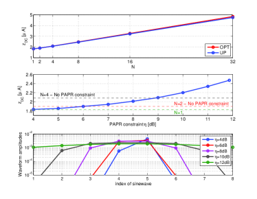
Figure 3: $z_{DC}$ as a function of $N$ (top) and PAPR constraint $\eta$ for $N=8$ (middle). WPT waveform amplitude as a function of $\eta$ for $N=8$ (bottom). No wireless channel is assumed, i.e. $A=1$ and $\bar{\psi}=0$, and $M=1$.

We now evaluate the performance of WPT waveforms in a single rectenna scenario representative of a WiFi-like environment at a center frequency of 5.18GHz with a 36dBm transmit power, isotropic transmit antennas (i.e. EIRP of 36dBm for $M=1$), 2dBi receive antenna gain and 58dB path loss in a large open space environment with a NLOS channel power delay profile with 18 taps obtained from model B [24]. Taps are modeled as i.i.d. circularly symmetric complex Gaussian random variables, each with an average power $\beta_{l}$. The multipath response is normalized such that $\sum_{l=1}^{18}\beta_{l}=1$. With one transmit antenna, this leads to an average received power of -20dBm ($10\mu W$). Equivalently, this system model can be viewed as a transmission over the aforementioned normalized multipath channel with an average transmit power fixed to -20dBm. The frequency gap is fixed as $\Delta_{w}=2\pi\Delta_{f}$ with $\Delta_{f}=B/N$ and $B=1,10$MHz. The $N$ sinewaves are centered around 5.18GHz.

In Fig 4, we illustrate the effect of frequency selectivity on the shape of the transmit waveform obtained using Algorithm 1. Fig 4 (top) illustrates the frequency response of one realization of the multipath channel over 1MHz and 10 MHz bandwidth. Fig 4 (bottom) displays the magnitude of the waveform optimized for $N=16$ (Algorithm 1) over such a channel realization. Interestingly, the optimized waveform has a tendency to allocate more power to frequencies exhibiting larger channel gains. This is reminiscent of the water-filling power allocation strategy in communication. This observation also suggests a suboptimal low complexity waveform design that would allocate power proportionally to the channel strength. For comparison, recall that the ASS waveform, motivated by the linear model, would allocate all power to the frequency corresponding to the strongest channel gain.

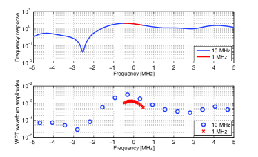
Figure 4: Frequency response of the wireless channel and WPT waveform magnitudes ($N=16$) for 1 MHz and 10 MHz bandwidths.

We now evaluate the performance gain of the adaptive optimized (OPT) waveform (Algorithm 1) versus three baselines: a non-adaptive waveform not relying on CSIT and two adaptive waveforms relying on CSIT but not requiring the optimization of Section IV. From the scaling law analysis, a suitable choice of non-adaptive waveform for single antenna WPT is UP. We therefore choose the non-adaptive baseline waveform as $\phi_{n,m}=0$ and $s_{n,m}=\sqrt{2P}/\sqrt{NM}$ $\forall n,m$. Motivated by the observations made in Fig 4, the first adaptive baseline waveform is chosen as a matched filter (MF) allocating power to all sinewaves but proportionally to the channel strength, i.e. $\phi_{n,m}=-\bar{\psi}_{n,m}$ and $s_{n,m}=cA_{n,m}$ with $c$ a constant to guarantee the power constraint. Hence the difference between the optimized waveform and the one based on MF lies in a different choice of amplitudes. The second adaptive baseline waveform is the ASS, designed according to the linear model.

Fig 5 and 6 display $z_{DC}$ averaged over many channel realizations as a function of $(N,M)$ for two bandwidths $B=1MHz$ and $B=10MHz$, respectively. We make the following observations. First, for small bandwidth ($B=1$MHz), the UP non-adaptive waveform performs pretty well in the presence of a single transmit antenna ($M=1$), confirming that for channels with little frequency selectivity, CSI feedback is not needed. On the other hand, for larger bandwidth ($B=10$MHz), the non-adaptive waveform is clearly outperformed by the adaptive waveforms, therefore highlighting the usefulness of CSI feedback in WPT even with a single transmit antenna. Second, for small bandwidth, the ASS waveform is significantly outperformed by the UP waveform for $M=1$, despite the fact it requires CSI knowledge at the Transmitter. For larger bandwidth, the ASS waveform benefits from the channel frequency selectivity to get close performance to OPT for small $N$. As $N$ increases, the ASS waveform is however clearly outperformed by the adaptive MF and OPT waveforms. This highlights the inaccuracy of the linear model in characterizing the rectifier and the inefficiency of the linear model-based design. The inefficiency is particularly severe as $N$ increases irrespectively of the bandwidth. These observations confirm the predictions made from the scaling laws in Table I. Third, OPT outperforms all waveforms in all configurations. Fourth, MF is a good alternative to OPT, at least with small bandwidth, and does not require any optimization. For larger bandwidth, OPT shows a non-negligible gain over MF as $N$ increases.

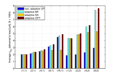
Figure 5: Average $z_{DC}$ as a function of $(N,M)$ with $B=1$MHz.

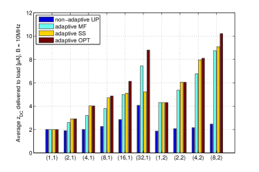
Figure 6: Average $z_{DC}$ as a function of $(N,M)$ with $B=10$MHz.

Fig 7 further analyzes the sensitivity of $z_{DC}$ to the bandwidth for a fixed number of sinewaves $N=16$ and various waveforms. Waveforms relying on uniform power allocation such as non-adaptive UP and adaptive UPMF experience some loss as the bandwidth increases and the channel becomes more frequency selective. On the other hand, adaptive OPT and adaptive SS benefit from the frequency selectivity by favouring the strongest sinewave(s). In [7], experiments show that waveforms with high peak to average power ratio (PAPR) increase RF-to-DC conversion efficiency. The conclusion was drawn for various waveforms (OFDM, white noise, chaotic) that were not designed or optimized for WPT. Following this observation, we investigate whether designing waveforms so as to maximize the PAPR at the input of the rectenna, after the wireless channel, is a suitable approach. The adaptive waveform MAX PAPR in Fig 7 is designed following this philosophy. It uses the same phases as OPT but inverts the channel such that at the input to the rectifier, the waveform appears as an in-phase multisine with uniform power allocation (which is known to have the maximum PAPR of $10\log_{10}\left(2N\right)$ dB). This is mathematically formulated by choosing $s_{n}^{2}=C/A_{n}^{2}$ where $C$ is a constant to satisfy the transmit power constraint. Results show that this is a rather inefficient waveform design strategy. This originates from the relatively low magnitude of the waveform peaks due to the excessive amount of power wasted in inverting the wireless power to guarantee the maximum PAPR at the input of the rectenna. Note also that non-adaptive UP would lead to the highest transmit PAPR (i.e. PAPR of the transmit waveform, before the wireless channel) due the uniform allocation across 16 in-phase sinewaves. OPT on the other hand has a transmit PAPR always lower than UP despite providing higher $z_{DC}$.

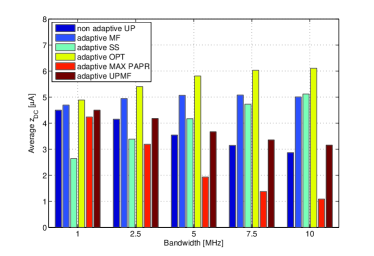
Figure 7: Effect of Bandwidth $B$ on $z_{DC}$ for $N=16$ and $M=1$.

Fig 8 further investigates the impact of PAPR on the performance of the optimized multisine waveforms. It considers the OPT waveform with 16 sinewaves uniformly spread over 3 different bandwidths. $z_{DC}$ is plotted against the PAPR of the transmit waveform for each realization of the multipath channel, along with some linear regression fit. It is noted that there is some positive correlation between $z_{DC}$ and PAPR, especially for small bandwidths. As the bandwidth increases and the wireless channel becomes more frequency selective, the optimized waveform has a tendency to allocate less power to the weakest channels, therefore leading to lower PAPR. This explains why as the bandwidth increases, the correlation between DC current and PAPR reduces.

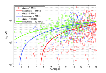
Figure 8: $z_{DC}$ versus transmit PAPR for $N=16$ and $M=1$.

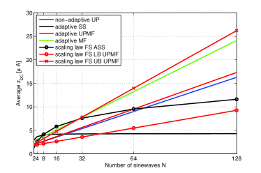
Figure 9: Effect of $N$ on $z_{DC}$ for $M=1$ and 5 MHz bandwidth.

Fig 9 reveals the performance of a large-scale multisine WPT using 4 suboptimal (though low complexity) waveforms (UP, ASS, UPMF and MF) for $M=1$ and 5 MHz bandwidth. The linear model-based ASS is significantly outperformed by the non-linear model-based design as $N$ grows large. The scaling laws for ASS and UPMF over frequency-selective (FS) channels in Table I are also displayed for comparison.

VI-B Accurate and Realistic Performance Evaluations

The second type of evaluations is based on an accurate modeling of the rectenna in PSpice in order to validate the waveform optimization and the rectenna non-linearity model. To that end, the waveforms after the wireless channel have been used as inputs to the realistic rectenna of Fig 10 designed for an input power of -20dBm. The circuit contains an L-matching network [3] to guarantee a good matching between the rectifier and the antenna and to minimize the impedance mismatch due to variations in frequency and input power level of the input signal. The values of the capacitor C1 and the inductor L1 are optimized to match the antenna impedance to the average input impedance of the rectifier resulting from an input signal composed of 4 sinewaves and spread across $B=10$MHz. Using ADS Harmonic Balance simulation, the rectifier impedance is measured at the 4 sinewave frequencies during a few iterations, and conjugate matching is performed to match the antenna to the average rectifier impedance at each iteration until the impedance mismatch error is minimised. $\textnormal{Vs}=v_{s}(t)=2y(t)\sqrt{R_{ant}}$ is set as the voltage source. Taking the optimized waveform as an example, for a given channel realization, Algorithm 1 is used to derive the optimal waveform weights, which are then used to generate in Matlab the waveform $y(t)$ as in (4) (after the wireless channel). Several periods of the signal are generated such that $t=0,\ldots,c\Delta_{t}$, with $c$ a positive integer chosen sufficiently large to make sure that the rectifier is in the steady-state response mode and $\Delta_{t}=1/\Delta_{f}$ the period of the waveform. Quantity $y(t)$ is stored and then fed into the PSpice circuit simulator to generate the voltage source Vs in Fig 10. The antenna and load impedances are set as $\textnormal{R1}=R_{ant}=50\Omega$ and $\textnormal{R2}=R_{L}=1600\Omega$, respectively. The output capacitor is chosen as $\textnormal{C2}=C_{out}=100$pF for $B=1$MHz and $\textnormal{C2}=C_{out}=10$pF for $B=10$MHz so that the output DC power is maximized and the rate of charge and discharge of $C_{out}$ is maintained in proportion to the period of the waveform, i.e. for evaluations with $B=1$MHz, C2 is replaced by a 100pF capacitor in Fig 10.

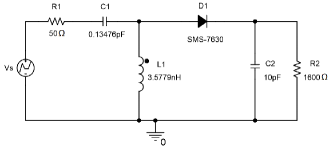
Figure 10: Rectenna with a single diode and a L-matching network used for PSpice evaluations with $B=10$MHz.

Fig 11 illustrates the increase of the harvested DC power as a function of $N$ for a single transmit antenna and assuming no wireless channel, i.e. $A=1$ and $\bar{\psi}=0$ (representing a frequency flat channel). The harvested DC power is not a monotonically increasing function contrary to what was observed in Fig 3 with $z_{DC}$. This is explained by the fact that the rectenna has been optimized for 4 sinewaves. For $B=10$MHz and $N=4$, $C_{out}=10$pF was found appropriate. Nevertheless, as $N$ increases, for a fixed $B$, $\Delta_{f}$ decreases, which affects the rate of charge and discharge of the output capacitor. This shows that $C_{out}$ (but also the load and the matching network) should ideally be adjusted as a function of $N$. We indeed notice that for large $N$, a larger capacitor of 100pF is better than 10pF. It is worth noting even if the rectenna design changes as a function of $N$, beyond a certain $N$, the peak of the voltage at the input of the diode would be higher than the diode breakdown voltage (2V for SMS7630), which would cause a sharp decrease in efficiency.

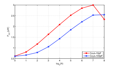
Figure 11: $P_{DC}$ as a function of $N$ for $B=10$MHz. No wireless channel is assumed, i.e. $A=1$ and $\bar{\psi}=0$, and $M=1$.

In Fig 12, considering the channel impulse response of Fig 4, we illustrate the time-domain evolution of the input and output voltages (in the form of $v_{s}(t)$ and $v_{out}(t)$) for the OPT and UP waveforms (with $N=16$ and $B=10$MHz). We also illustrate the effect of the output capacitance $C_{out}$ on the performance. Large peaks in the input voltage occur with a periodicity $\Delta_{t}=1/\Delta_{f}=N/B=1.6\mu$s. Output voltage is not flat contrary to what is expected with an ideal rectifier (as used in the non-linear model of Section III). This is due to the finite $R_{L}C_{out}$ chosen in the simulated (and optimized) rectifier of Fig 10. We note that a larger $C_{out}$ leads to a smoother output voltage and a better discharging behaviour but a slower charging time and lower output peak voltages. A good value for $C_{out}$ results from a compromise between those conflicting mechanisms that explains why a finite $C_{out}$ is needed in practice. We also note that the OPT waveform leads to a higher output voltage than that obtained with the UP waveform. The harvested DC output power with $C_{out}=100$pF is given by $2.3281\mu$W and $6.4157\mu$W, for UP and OPT, respectively. With $C_{out}=10$pF, the harvested DC output power is slightly higher and given by $2.9435\mu$W and $6.9387\mu$W, respectively.

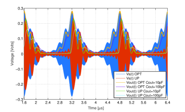
Figure 12: $v_{s}(t)$ and $v_{out}(s)$ over the wireless channel of Fig 4 with OPT and UP waveforms for $N=16$, $B=10$ MHz and $C_{out}=10$pF,100pF.

Fig 13 and 14 display the average harvested DC output power for $B=1$MHz and $B=10$MHz (using the same channel realizations as those used in Fig 5 and 6), respectively. We make important observations. First, the results confirm the observations made in Fig 5 and 6 and validate the rectenna non-linearity model and the waveform optimization. There is indeed a good match between the behavior predicted from the analytical nonlinear model and the one observed from the PSpice simulations. Second, they highlight the significant (and increasing as $N,M$ grow) gains achieved by the nonlinear model-based design over the linear model-based design. Third, they highlight that the linear model does not characterize correctly the rectenna behavior, which leads to an inefficient multisine waveform design. Indeed, if the linear model had accurately characterized the rectifier behavior, the ASS waveform would have provided the highest average DC power over all other waveforms. It is clearly not the case. The behaviour observed from Fig 13 and 14 cannot be explained based on the linear model. In Fig 13, with $M=1$, ASS (requiring CSIT) is even outperformed by non-adaptive UP (not requiring CSIT).

Results in Fig 13 and 14 can also be viewed in terms of RF-to-DC conversion efficiency by dividing the harvested DC power by the average input power ($10\mu W$). For 10MHz and $M=1$, the RF-to-DC conversion efficiency of the OPT waveform is 9%, 15%, 22%, 28%, 37% and 46% for $N=1,2,4,8,16$ and 32, respectively.

It is worth noting in Fig 13 and 14 the effect of bandwidth on average DC power. The average DC power with a 10 MHz bandwidth is larger than that with a 1 MHz bandwidth. This comes from the increased channel frequency selectivity and the diode being turned on more often as $\Delta_{f}$ increases. When $N=1$, all waveforms obviously achieve the same performance.

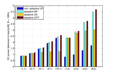
Figure 13: Average DC power as a function of $(N,M)$ with $B=1$MHz.

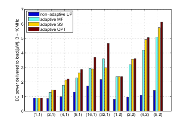
Figure 14: Average DC power as a function of $(N,M)$ with $B=10$MHz.

Remark 5

$n_{o}=4$ was used throughout the waveform design and $z_{DC}$ evaluations. More investigations are needed to assess the usefulness of even higher order terms ($n_{o}\geq 6$). In [6], it was claimed that $n_{o}=4$ is the minimum order required to characterize the nonlinear mechanisms of the diode.

VII Conclusions and Future Works

The paper looks at a WPT link optimization and derives a methodology to design and optimize multisine waveforms for WPT. Assuming the CSI is available to the transmitter, the waveforms result from a non-convex posynomial maximization problem and are shown through realistic simulations to provide significantly higher harvested DC power over various baseline waveforms under a fixed transmit power constraint. The results show the importance of accounting for the non-linearity of the rectifier in any design involving wireless power.

Due to the space limitation, there are many important and exciting research avenues unaddressed in this paper and left for future work. Some of them are highlighted below.

The waveform design problem addressed in this paper assumes $N$ sinewaves with a uniform frequency spacing $\Delta_{f}=B/N$ for a given spectrum bandwidth $B$. A fundamental question arising from this work is, given a spectrum bandwidth $B$, what is the best way to transmit power so as to maximize the output DC power? This would help understanding how to make the best use of the RF spectrum for WPT. This problem has been investigated for several decades in wireless communication but is an uncharted area in WPT.

The work highlights the usefulness of adaptive waveforms and CSIT. The fundamentals of CSI acquisition/feedback in WPT remain largely unknown. Some interesting ideas along this line have appeared in [23]. However, the work relied on the linear model. It is unclear yet whether a similar approach can be used over the non-linear wireless power channel.

The scaling laws and evaluations highlight the potentials of a promising architecture relying on large-scale multisine multi-antenna waveforms dedicated to WPT. This architecture would be to wireless power what massive MIMO is to communication. More results along this line can be found in [25].

The work also highlights the importance of understanding and modeling the wireless power channel and formulating a complete link optimization (transmitter to rectenna) in order to design an efficient WPT architecture. Since WPT is the fundamental building block of various types of wireless powered systems (e.g. WPT, SWIPT, WPCN, backscatter communication), this motivates a bottom-up approach where any wireless powered system is based on a sound science-driven design of the underlying WPT. The waveform design and the rectifier non-linearity tackled in this paper therefore have direct consequences on the design of SWIPT, WPCN and backscatter communication. For instance, some preliminary results on SWIPT waveforms have been reported in [26], where it is shown that the superposition of multisine and OFDM waveforms enlarges the rate-energy region compared to an OFDM-only transmission. This originates from the non-linearity of the rectifier and the fact that the OFDM waveform, due to the randomness of the information, is less efficient than a (deterministic) multisine waveform to convert RF power to DC power.

References

- [1] B. Clerckx, E. Bayguzina, D. Yates, and P.D. Mitcheson, “Waveform Optimization for Wireless Power Transfer with Nonlinear Energy Harvester Modeling,” IEEE ISWCS 2015, August 2015, Brussels, arXiv:1506.08879.
- [2] H.J. Visser, R.J.M. Vullers, “RF Energy Harvesting and Transport for Wireless Sensor Network Applications: Principles and Requirements,” Proceedings of the IEEE, Vol. 101, No. 6, June 2013.
- [3] M. Pinuela, P. Mitcheson and S. Lucyszyn, “Ambient RF energy harvesting in urban and semi-urban environments,” IEEE Trans. on Microw. Theory and Techn., vol 61, no 7, july 2013.
- [4] J.A. Hagerty, F.B. Helmbrecht, W.H. McCalpin, R. Zane, and Z.B. Popovic, “Recycling Ambient Microwave Energy with Broad-Band Rectenna Arrays,” IEEE Trans. MTT, vol 52, no 3, March 2004.
- [5] M.S. Trotter, J.D. Griffin and G.D. Durgin, “Power-Optimized Waveforms for Improving the Range and Reliability of RFID Systems,” 2009 IEEE International Conference on RFID.
- [6] A. S. Boaventura and N. B. Carvalho, “Maximizing DC Power in Energy Harvesting Circuits Using Multisine Excitation,” 2011 IEEE MTT-S International Microwave Symposium Digest (MTT).
- [7] A. Collado and A. Georgiadis, “Optimal Waveforms for Efficient Wireless Power Transmission,” IEEE Microwave and Wireless Components Letters, vol. 24, no.5, May 2014.
- [8] S. Wetenkamp, “Comparison of single diode vs. dual diode detectors for microwave power detection,” in IEEE MTT-S Int. Microw. Symp. Dig., Boston, MA, USA, 1983, pp. 361-363.
- [9] X. Zhou, R. Zhang and C. K. Ho, “Wireless Information and Power Transfer: Architecture Design and Rate-Energy Tradeoff,” IEEE Trans. on Commun., vol. 61, no. 11, pp. 4754-4767, Nov 2013.
- [10] B. Clerckx and C. Oestges, “MIMO Wireless Networks: Channels, Techniques and Standards for Multi-Antenna, Multi-User and Multi-Cell Systems,” Academic Press (Elsevier), Oxford, UK, Jan 2013.
- [11] J.-P. Curty, N. Joehl, F. Krummenacher, C. Dehollain, and M.J. Declercq, “A Model for -Power Rectifier Analysis and Design,” IEEE Trans. on Circuits and Systems-I, vol. 52, no. 12, pp. 2771-2779, Dec. 2005.
- [12] A. Boaventura, A. Collado, N. B. Carvalho, A. Georgiadis, “Optimum behavior: wireless power transmission system design through behavioral models and efficient synthesis techniques”, IEEE Microwave Magazine, vol. 14, no. 2, pp. 26-35, March/Apr. 2013.
- [13] S. Ladan and K. Wu, “Nonlinear Modeling and Harmonic Recycling of Millimeter-Wave Rectifier Circuit,” IEEE Trans. MTT, vol. 63, no. 3, March 2015.
- [14] K. Huang and E, G. Larsson, “Simultaneous information and power transfer for broadband wireless systems,” IEEE Trans. Sig. Proc., vol. 61, no. 23, pp. 5972-5986, Dec. 2013.
- [15] Z.B. Zawawi, J. Park and B. Clerckx, “Simultaneous Wireless Information and Power Transfer in a Two-User OFDM Interference Channel,” IEEE ISWCS 2015, August 2015, Brussels.
- [16] I.S. Gradshteyn, I.M. Ryzhik, “Table of Integrals, Series, and Products,” seventh edition, Academic Press, 2007.
- [17] M. Chiang, “Geometric Programming for Communication Systems,” Foundations and Trends in Communications and Info. Theory, 2005.
- [18] R.J. Duffin and E.L. Peterson, “Geometric Programming with Signomials,” J. of Optimization Theory and Applications, Vol. 11, No. 1, 1973.
- [19] C.S. Beightler and D.T. Philips, “Applied Geometric Programming,” Wiley, 1976.
- [20] M. Grant, S. Boyd, and Y. Ye, “CVX: MATLAB software for disciplined convex programming [Online],” Available: http://cvxr.com/cvx/, 2015.
- [21] B.R. Marks and G.P. Wright, “A general inner approximation algorithm for nonconvex mathematical programs,” Operations Research, vol. 26, no. 4, pp. 681-683, 1978.
- [22] M. Chiang, C.W. Tan, D.P. Palomar, D. ONeill, and D. Julian, “Power Control By Geometric Programming,” IEEE Trans. on Wireless Comm., Vol. 6, No. 7, pp. 2640-2651, July 2007.
- [23] J. Xu and R. Zhang, “Energy Beamforming With One-Bit Feedback,” IEEE Trans. on Sig. Proc., Vol. 62, No. 20, pp. 5370-5381 , Oct. 2014.
- [24] J. Medbo, P. Schramm, “Channel Models for HIPERLAN/2 in Different Indoor Scenarios,” 3ERI085B, ETSI EP BRAN, March 1998.
- [25] Y. Huang and B. Clerckx, “Waveform Optimization for Large-Scale Multi-Antenna Multi-Sine Wireless Power Transfer,” IEEE SPAWC 2016, arXiv:1605.01191.
- [26] B. Clerckx, “Waveform Optimization for SWIPT with Nonlinear Energy Harvester Modeling,” 20th International ITG Workshop on Smart Antennas (WSA 2016), March 2016, Munich, arXiv:1602.01061.