Chiral matrix model of the semi-Quark Gluon Plasma in QCD

Abstract

Previously, a matrix model of the region near the transition temperature, in the “semi”-Quark Gluon Plasma, was developed for the theory of $SU(3)$ gluons without quarks. In this paper we develop a a chiral matrix model applicable to QCD by including dynamical quarks with $2+1$ flavors. This requires adding a nonet of scalar fields, with both parities, and coupling these to quarks through a Yukawa coupling, $y$. Treating the scalar fields in mean field approximation, the effective Lagrangian is computed by integrating out quarks to one loop order. As is standard, the potential for the scalar fields is chosen to be symmetric under the flavor symmetry of $SU(3)_{L}\times SU(3)_{R}\times Z(3)_{A}$, except for a term linear in the current quark mass, $m_{qk}$. In addition, at a nonzero temperature $T$ it is necessary to add a new term, $\sim m_{qk}\,T^{2}$. The parameters of the gluon part of the matrix model are identical to that for the pure glue theory without quarks. The parameters in the chiral matrix model are fixed by the values, at zero temperature, of the pion decay constant and the masses of the pions, kaons, $\eta$, and $\eta^{\prime}$. The temperature for the chiral crossover at $T_{\chi}=155$ MeV is determined by adjusting the Yukawa coupling $y$. We find reasonable agreement with the results of numerical simulations on the lattice for the pressure and related quantities. In the chiral limit, besides the divergence in the chiral susceptibility there is also a milder divergence in the susceptibility between the Polyakov loop and the chiral order parameter, with critical exponent $\beta-1$. We compute derivatives with respect to a quark chemical potential to determine the susceptibilities for baryon number, the $\chi_{2n}$. Especially sensitive tests are provided by $\chi_{4}-\chi_{2}$ and by $\chi_{6}$, which changes in sign about $T_{\chi}$. The behavior of the susceptibilities in the chiral matrix model strongly suggests that as the temperature increases from $T_{\chi}$, that the transition to deconfinement is significantly quicker than indicated by the measurements of the (renormalized) Polyakov loop on the lattice.

I Introduction

Our understanding of the behavior of the collisions of heavy nuclei at ultra-relativistic energies rests upon the bedrock provided by numerical simulations of lattice QCD. At present, for QCD with $2+1$ light flavors, these simulations provide us with results, near the continuum limit, for the behavior of QCD in thermodynamic equilibrium Boyd et al. (1995); *umeda_fixed_2009; *borsanyi_precision_2012; Cheng et al. (2006); *cheng_qcd_2008; *bazavov_equation_2009; *cheng_equation_2010; *bazavov_chiral_2012; Bazavov and Petreczky (2013); Bazavov et al. (2016); Buchoff et al. (2014); Bhattacharya et al. (2014); Bazavov et al. (2014); Ding et al. (2015); Cheng et al. (2009); *bazavov_fluctuations_2012; *bazavov_freeze-out_2012; Aoki et al. (2006); *fodor_phase_2009; *aoki_qcd_2009; *borsanyi_qcd_2010; *borsanyi_is_2010; *durr_lattice_2011; *endrodi_qcd_2011; Borsanyi et al. (2014a, 2012b); *bellwied_is_2013; *borsanyi_freeze-out_2013; *borsanyi_freeze-out_2014; *bellwied_fluctuations_2015; Ratti (2016). Most notably, that there is a chiral crossover at a temperature of $T_{\chi}\sim 155\pm 9$ MeV.

While this understanding is essential, there are many quantities of experimental interest which are much more difficult to obtain from numerical simulations of lattice QCD. This includes all quantities which enter when QCD is out of but near thermal equilibrium, such as transport coefficients, the production of dileptons and photons, and energy loss.

For this reason, it is most useful to have phenomenological models which would allow us to estimate such quantities. Lattice simulations demonstrate that in equilibrium, a non-interacting gas of hadrons works well up to rather high temperatures, about $\sim 130$ MeV Boyd et al. (1995); *umeda_fixed_2009; *borsanyi_precision_2012; Cheng et al. (2006); *cheng_qcd_2008; *bazavov_equation_2009; *cheng_equation_2010; *bazavov_chiral_2012; Bhattacharya et al. (2014); Bazavov et al. (2014); Ding et al. (2015); Cheng et al. (2009); *bazavov_fluctuations_2012; *bazavov_freeze-out_2012; Aoki et al. (2006); *fodor_phase_2009; *aoki_qcd_2009; *borsanyi_qcd_2010; *borsanyi_is_2010; *durr_lattice_2011; *endrodi_qcd_2011; Borsanyi et al. (2014a, 2012b); *bellwied_is_2013; *borsanyi_freeze-out_2013; *borsanyi_freeze-out_2014; *bellwied_fluctuations_2015; Ratti (2016). Similarly, resummations of perturbation theory, such as using Hard Thermal Loops (HTL’s) at Next to- Next to- Leading order (NNLO), work down to about $\sim 300$ or $\sim 400$ MeV Andersen et al. (2010a); *andersen_gluon_2010; *andersen_nnlo_2011; *andersen_three-loop_2011; *haque_two-loop_2013; *mogliacci_equation_2013; *haque_three-loop_2014. What is difficult to treat is the region between $\sim 130$ and $\sim 300-400$ MeV, which has been termed the “sQGP”, or strong Quark-Gluon Plasma. This name was suggested by T. D. Lee, because analysis of heavy experiments appears to show that the ratio of the shear viscosity to the entropy density, $\eta/s$, is very small. For QCD, in perturbation theory $\eta/s\sim 1/g^{4}$, and so a small value of $\eta/s$ suggests that the QCD coupling constant, $g$, is large.

There is another way of obtaining a small value of $\eta/s$ without assuming strong coupling Pisarski (2000); *dumitru_degrees_2002; *dumitru_two-point_2002; *scavenius_k_2002; *dumitru_deconfining_2004; *dumitru_deconfinement_2005; *dumitru_dense_2005; *oswald_beta-functions_2006; Pisarski (2006). At high temperature, the quarks and gluons are deconfined, and their density can be estimated perturbatively. At low temperatures, confinement implies that the density of particles with color charge vanishes as $T\rightarrow 0$. Numerical simulations demonstrate that even with dynamical quarks, the density of color charge, as measured by the expectation value of the Polyakov loop, is rather small at $T_{\chi}$, with $\langle\ell\rangle\sim 0.1$. This presumes that the Polyakov loop is normalized so that its expectation value approaches one at infinite temperature, $\langle\ell\rangle\rightarrow 1$ as $T\rightarrow\infty$.

Because of the decrease in the density of color charge, the region about $T_{\chi}$ can be termed not as a strong, but as a “semi”-QGP. In this view, the dominant physics is assumed to be the partial deconfinement of color charge, analogous to partial ionization in Abelian plasmas Hidaka and Pisarski (2008); *hidaka_hard_2009; *hidaka_zero_2009; *hidaka_small_2010.

This partial deconfinement can be modeled in a matrix model of the semi-QGP. In such a matrix model, both the shear viscosity and the entropy density decrease as the density of color charges decreases. It is not obvious, but calculation shows that the shear viscosity vanishes quicker than the entropy density, so that the ratio $\eta/s\sim\langle\ell\rangle^{2}$ Hidaka and Pisarski (2008); *hidaka_hard_2009; *hidaka_zero_2009; *hidaka_small_2010. Thus in a matrix model, it is possible to obtain a small shear viscosity not because of strong coupling, but because the density of color charge is small.

A matrix model of the semi-QGP has been developed for the pure gauge theory Dumitru and Smith (2008); *smith_effective_2013; Dumitru et al. (2011, 2012); Sasaki and Redlich (2012); Dumitru et al. (2014). The fundamental variables are the eigenvalues of the thermal Wilson line, and it is based upon the relationship between deconfinement and the spontaneous breaking of the global $Z(N_{c})$ symmetry of a $SU(N_{c})$ gauge theory. This model is soluble in the limit for a large number of colors, and exhibits a novel “critical first order” phase transition Pisarski and Skokov (2012); *lin_zero_2013. With heavy quarks, it has been used to compute the critical endpoint for deconfinement Kashiwa et al. (2012) and properties of the Roberge-Weiss transition Kashiwa and Pisarski (2013). The production of dileptons and photons has also been computed Gale et al. (2015); *hidaka_dilepton_2015; *satow_chiral_2015; the suppression of photon production in the semi-QGP may help to understand the experimentally measured azimuthal anisotropy of photons. In a matrix model, collisional energy loss behaves like the shear viscosity, and is suppressed as the density of color charges decreases Lin et al. (2014).

In this paper we develop a chiral matrix model by including light, dynamical quarks, as is relevant for QCD with $2+1$ light flavors. Our basic assumption is the following. The global $Z(3)$ symmetry of a pure $SU(3)$ gauge theory is broken by the presence of dynamical quarks, and generate a nonzero expectation value for the Polyakov loop at nonzero temperature, $\langle\ell\rangle\neq 0$ when $T\neq 0$. As noted above, however, this expectation value is remarkably small at the chiral transition, with $\langle\ell\rangle\sim 0.1$. Thus in QCD, the breaking of the global $Z(3)$ symmetry by dynamical quarks is surprisingly weak near $T_{\chi}$. This is a nontrivial result of the lattice: it is related to the fact that in the pure gauge theory, the deconfining phase transition occurs at $T_{d}\sim 270$ MeV, which is much higher than $T_{\chi}\sim 155$ MeV. We do not presume that this holds for arbitrary numbers of colors and flavors. In QCD, though, it suggests that treating the global $Z(3)$ symmetry breaking as small, and the matrix degrees of freedom as “relevant”, is a reasonable approximation.

Other than that, while the technical details are involved, the basic physics is simple. We start with a standard chiral Lagrangian for the nonet of light pseudo-Goldstone mesons: pions, kaons, $\eta$, and the $\eta^{\prime}$. Because we wish to analyze the chirally symmetric phase, we add a nonet of mesons with positive parity, given by the sigma meson and its associated partners ’t Hooft (1986); Donoghue et al. (1992); Lenaghan et al. (2000); Roeder et al. (2003); *janowski_glueball_2011; *parganlija_meson_2013; Stiele and Schaffner-Bielich (2016); Jaffe (1977); *black_mechanism_2000; *close_scalar_2002; *jaffe_diquarks_2003; *maiani_new_2004; *pelaez_light_2004; *t_hooft_theory_2008; *pelaez_controversy_2015. The field for the mesons, $\Phi$, couples to itself through a Lagrangian which includes terms which are invariant under the flavor symmetry of $SU(3)_{L}\times SU(3)_{R}\times U_{A}(1)$.

For the meson field $\Phi$ we take a linear sigma model, as then it is easy to treat the chirally symmetric phase (this is possible, but more awkward, with a nonlinear sigma model). We include a chirally symmetric Yukawa coupling between $\Phi$ and the quarks, with a Yukawa coupling constant $y$. The quarks are integrated out to one loop order, while the meson fields are treated in the mean field approximation, neglecting their fluctuations entirely. Dropping mesonic fluctuations is clearly a drastic approximation, but should be sufficient for an initial study of the matrix model.

To make the pions and kaons massive, we add a term which is linear in the current quark mass, $m_{qk}$. We demonstrate that in order for the constituent mass of the quarks to approach the current quark mass at high temperature, it is also necessary to add an additional term $\sim m_{qk}$: this new term vanishes at zero temperature, but dominates at high temperature. This new term has not arisen previously, because typically linear sigma models do not include fluctuations of the quarks.

The meson potential includes chirally symmetric terms for $\Phi$ at quadratic, cubic, and quartic order. For three flavors, the cubic term represents the effect of the axial anomaly. The parameters of the model are fixed by comparing to the meson masses at zero temperature, for the masses of the pion, kaon, $\eta$, and $\eta^{\prime}$, and the pion decay constant. This fitting is typical of models at zero temperature. The quartic term includes a novel logarithmic term from the fluctations of the quarks, but this does not markedly change the parameters of the potential for $\Phi$.

The chiral matrix model can be considered as a generalization of Polyakov loop models, as first proposed by Fukushima Fukushima (2004); *fukushima_phase_2011; *fukushima_phase_2013; Sasaki et al. (2007); Skokov et al. (2010a, b); *morita_role_2011; Islam et al. (2015); Ishii et al. (2016); Miyahara et al. (2016); see also Schaefer and Wagner (2012a); *schaefer_qcd_2012; *chen_chemical_2015; *berrehrah_quark_2015; *tawfik_su3_2015; *tawfik_polyakov_2015. In a Polyakov loop model, the gauge fields are integrated out to obtain an effective model of the Polyakov loop and hadrons. Because of this, except for one special case (dilepton production at leading order Islam et al. (2015)), Polyakov loop models can only be used to study processes in, and not near, equilibrium. In a matrix model, though, as $A_{0}$, is not integrated out it is straightforward to compute processes neat equilibrium by analytic continuation. This includes many quantities of experimental relevance, especially transport coefficients such as shear and bulk viscosities.

There is another difference between the two models. In a Polyakov loop model, all thermodynamic functions are functions of the ratio $T/T_{c}$, where $T_{c}$ is the critical temperature. In a pure gauge theory, $T_{c}$ is the temperature for the deconfining phase transition, $T_{d}$. With dynamical quarks, $T_{c}$ is that for the restoration of chiral symmetry, $T_{\chi}$.

In contrast, in our chiral matrix model we take the gluon potential to be identical to that of the pure gauge theory, keeping the parameter $T_{d}=270$ MeV. The Yukawa coupling $y$ is then tuned to obtain a chiral crossover temperature $T_{\chi}=155$ MeV. We stress that in our model, $T_{d}$ is not the temperature for deconfinement in QCD: it is just a parameter of the gluon part of the effective, nonperturbative potential for $A_{0}$. Since dynamical quarks explicitly break the global $Z(3)$ symmetry of the pure gauge theory, there is no precise definition of a deconfining temperature in QCD. One approximate measure is provided by susceptibilities involving the Polyakov loop, as considered in Sec. (V.5). These indicate that deconfinement occurs close to $T_{\chi}$, Fig. (9).

There are other models in which transport coefficients can be computed. These include Polyakov quark meson models improved by using the functional renormalization group Braun et al. (2010); Herbst et al. (2011); *fister_confinement_2013; *herbst_phase_2013; *haas_gluon_2014; *herbst_thermodynamics_2014; *mitter_chiral_2015; Herbst et al. (2015); Fu and Pawlowski (2015a, b).

As a byproduct we make some observations about linear sigma models. For the special limit of three degenerate but massive flavors, in a general linear sigma model, we show that at zero temperature the difference of the masses squared of the singlet and octet states $0^{-}$ states equals the difference of the masses squared between the octet and singlet states for the $0^{+}$, Eq. (91). This is identical to the same relation for two degenerate, massive flavors ’t Hooft (1986).

To fix the parameters of the chiral matrix model, we only use properties of the $0^{-}$ nonet, not the $0^{+}$ nonet. This is fortunate, because the lightest $0^{+}$ nonet may be formed not from a quark antiquark pair, but is a tetraquark, composed of a diquark and diantiquark pair Jaffe (1977); *black_mechanism_2000; *close_scalar_2002; *jaffe_diquarks_2003; *maiani_new_2004; *pelaez_light_2004; *t_hooft_theory_2008; *pelaez_controversy_2015.

In this paper we do not consider a nonzero quark density, $\mu$. (We do consider derivatives of the pressure with respect to $\mu$, but these are then always evaluated at $\mu=0$.) Because at $\mu=0$ lattice simulations indicate that $T_{\chi}\ll T_{d}$, as one moves out in the plane of temperature and chemical potential, a quarkyonic phase in which $T_{\chi}<T_{d}$ when $\mu\neq 0$ McLerran and Pisarski (2007); *andronic_hadron_2010; *kojo_quarkyonic_2010; *kojo_interweaving_2012 is very natural in a chiral matrix model.

II Simple example of a chiral matrix model

Before diving into all of the technicalities associated with the chiral matrix model for $2+1$ flavors, it is useful to illustrate some general ideas in the context of a simple toy model. We take a single flavor of a Dirac fermion, interacting with a sigma field $\sigma$ through the Lagrangian

$${\cal L}=\overline{\psi}\left(\,\not\!\partial\,+\,y\,\sigma\right)\psi+\frac{m_{\sigma}^{2}}{2}\,\sigma^{2}+\frac{\lambda}{4}\,\sigma^{4}\;.$$ (1)

To demonstrate our points we can even neglect the coupling to the gauge field, although of course it is the coupling to gluons which drives chiral symmetry breaking. We neglect the kinetic term for the $\sigma$ field, since that will not enter into our analysis, which is entirely at the level of a mean field approximation for $\sigma$.

Notice that we include both the Lagrangian for the fermion $\psi$ as well as for the scalar field $\sigma$. Usually in sigma models, one assumes that the quarks are integrated out, with their interactions subsumed into those of the mesons. We cannot do that, because we need to include the effects of the quarks on the matrix model, as we show in the next Section. Consequently, we also include a Yukawa coupling $y$ between the fermion $\psi$ and $\sigma$.

This Lagrangian is invariant under a discrete chiral symmetry of $Z(2)$,

$$\psi\rightarrow\gamma_{5}\;\psi\;\;\;,\;\;\;\sigma\rightarrow-\,\sigma\;.$$ (2)

We take a Euclidean metric, where each Dirac matrix $\gamma^{\mu}$ satisfies $(\gamma^{\mu})^{2}=+1$, and $\gamma_{5}=\gamma_{0}\gamma_{1}\gamma_{2}\gamma_{3}$, so $\gamma_{5}^{2}=1$.

Integrating out the fermion gives the effective potential

$${\cal V}^{{\rm eff}}_{\sigma}=+\frac{m_{\sigma}^{2}}{2}\,\sigma^{2}+\frac{\lambda}{4}\,\sigma^{4}-\frac{1}{V}\,{\rm tr}\,{\rm log}\left(\not\!\partial+\,y\,\sigma\right)\;,$$ (3)

where $V$ is the volume of spacetime.

We thus need to compute the fermion determinant in the background field of the $\sigma$ field, which in mean field approximation we take to be constant. For ease of notation, we write

$$m_{f}=y\,\sigma\;.$$ (4)

Taking two derivatives with respect to $m_{f}^{2}$,

$$-\;\frac{\partial^{2}}{(\partial m_{f}^{2})^{2}}\;{\rm tr}\,\log(\;/\!\!\!\partial+m_{f})=+2\;{\rm tr}\;\frac{1}{(K^{2}+m_{f}^{2})^{2}}\;.$$ (5)

where $\partial_{\mu}=-iK^{\mu}$. Here the trace is the integral over the momentum $K$ in $4-2\epsilon$ dimensions,

$${\rm tr}=\widetilde{M}^{2\epsilon}\int\frac{d^{4-2\epsilon}K}{(2\pi)^{4-2\epsilon}}\;.$$ (6)

A renormalization mass scale $\widetilde{M}$ is introduced so that the trace has dimensions of mass⁴. The result is

$${\rm tr}\;\frac{1}{(K^{2}+m_{f}^{2})^{2}}=\;+\;\frac{1}{16\pi^{2}}\left(\frac{1}{\epsilon}+\log\left(\frac{\widetilde{M}^{2}}{m_{f}^{2}}\right)+\log(4\pi)-\gamma\right)\;,$$ (7)

where $\gamma\sim 0.577$ is the Euler-Mascheroni constant. Integrating with respect to $m_{f}^{2}$,

$$-\,\frac{1}{V}\,{\rm tr}\,\log(\;/\!\!\!\partial+m_{f})=+\frac{m_{f}^{4}}{16\pi^{2}}\left(\frac{1}{\epsilon}+\log\left(\frac{\widetilde{M}^{2}}{m_{f}^{2}}\right)+\log(4\pi)-\gamma+\frac{3}{2}\right)\;.$$ (8)

Defining

$$\log(M^{2})=\log\widetilde{M}^{2}+\log(4\pi)-\gamma+\frac{3}{2}\;,$$ (9)

we find

$$-\,\frac{1}{V}\,{\rm tr}\,\log(\;/\!\!\!\partial+m_{f})=+\frac{m_{f}^{4}}{16\pi^{2}}\left(\frac{1}{\epsilon}+\log\left(\frac{M^{2}}{m_{f}^{2}}\right)\right)\;.$$ (10)

The integral in Eq. (7) is logarithmically divergent, $\sim d^{4-2\epsilon}K/(K^{2}+m_{f}^{2})^{2}$. The divergence in the ultraviolet produces the usual factor of $1/\epsilon$ in $4-2\epsilon$ dimensions. Similarly, there is a logarithmic infrared divergence, cut off by the mass $m_{f}$.

We add a counterterm $\sim 1/\epsilon$ to the effective Lagrangian so that the sum with the one loop fermion determinant is finite. We thus obtain a renormalized effective Lagrangian,

$${\cal V}_{\sigma}^{{\rm eff,ren}}=+\frac{m_{\sigma}^{2}}{2}\,\sigma^{2}+\frac{1}{4}\,\left(\lambda+\,\frac{y^{4}}{4\,\pi^{2}}\log\left(\frac{M^{2}}{y^{2}\,\sigma^{2}}\right)\right)\sigma^{4}\;.$$ (11)

This is resembles the standard effective Lagrangian, except that it is no longer purely a polynomial in $\sigma$, but also has a term $\sim-\,y^{4}\,\sigma^{4}\log(\sigma^{2})$.

While this logarithmic term changes the effective Lagrangian, it does not really cause any particular difficulty. As usual we tune the scalar mass squared $m_{\sigma}^{2}$ to be negative at zero temperature, so that $\sigma$ develops a vacuum expectation value $\langle\sigma\rangle\neq 0$, and the fermion acquires a constituent mass $m_{f}=y\langle\sigma\rangle$. Because the chiral symmetry is discrete there are no (pseudo-) Goldstone bosons, but for the points we wish to make here this is irrelevant.

There is one feature which we must note. The sign of the logarithmic term in the effective Lagrangian, $\sim-\,y^{4}\,\sigma^{4}\,\log(\sigma^{2})$, is negative. This means that the quartic term is positive for small values of $\sigma$, so to obtain chiral symmetry breaking, we must tune $m_{\sigma}^{2}$ to be negative. That is no problem, but it also implies that for large values of $\sigma$, the potential is unbounded from below, as the logarithmic term $\sim-\,y^{4}\,\sigma^{4}\,\log(\sigma^{2})$ inevitably wins over $\sim+\,\lambda\,\sigma^{4}$.

It is useful to contrast this to the Gross-Neveu model in $1+1$ spacetime dimensions Gross and Neveu (1974). In this model there is a potential term $\sigma^{2}$, and from the one loop fermion determinant, a term $\sim+\,\sigma^{2}\,\log(\sigma^{2})$. Because the sign of logarithmic term is positive, the potential is unstable at small $\sigma$, which implies that there is chiral symmetry breaking for any value of the coupling constant. Conversely, the total potential is stable at large values of $\sigma$. This is opposite what happens in our effective model in $3+1$ dimensions.

The reason for this difference is clear: the Gross-Neveu model is asymptotically free Gross and Neveu (1974), while our model is infrared free. As such, we do not expect our theory to be well behaved at arbitrarily high momenta, which as an effective model is hardly surprising. It does imply that we need to check that we do not obtain results in a regime where there is instability, which we do. For the chiral matrix model which is applicable to QCD, this is easy to satisfy, because $\lambda$ is rather large, $y$ relatively small, and we never probe large $\sigma$. We comment that a similar instability at large $\sigma$ is present in renormalization group optimized perturbation theory Kneur and Neveu (2013); *kneur_chiral_2015; *kneur_scale_2015; *kneur_renormalization_2015.

The restoration of chiral symmetry at nonzero temperature is straightforward. In the imaginary time formalism, the four momenta $K^{\mu}=(k_{0},\vec{k})$, $k=|\vec{k}|$, where for a fermion the energy $k_{0}=(2n+1)\pi T$ for integral “$n$”. The trace is

$${\rm tr}=T\sum_{n=-\infty}^{+\infty}\widetilde{M}^{2\epsilon}\int\frac{d^{3-2\epsilon}k}{(2\pi)^{3-2\epsilon}}\;.$$ (12)

Computing the fermion determinant to one loop order with $m_{f}=y\,\sigma\ll T$,

$$-\,\frac{1}{V}\,{\rm tr}\,\log(\;/\!\!\!\partial+m_{f})\approx\frac{1}{12}\;y^{2}\,T^{2}\,\sigma^{2}+\frac{y^{4}}{16\pi^{2}}\,\sigma^{4}\left(\frac{1}{\epsilon}+\log\left(\frac{M^{2}}{T^{2}}\right)\right)+\ldots$$ (13)

From the term quadratic in $\sigma$, we see that there is a second order chiral phase transition at a temperature

$$T_{\chi}^{2}=-12\;\frac{m_{\sigma}^{2}}{y^{2}}\;,$$ (14)

which is standard.

What is also noteworthy are the subleading terms in the fermion determinant. At zero temperature we saw that there is a logarithmic term from an infrared divergence, $\sim\sigma^{4}\,\log(\sigma^{2})$. Eq. (13) shows that the logarithm of $\sigma$ does not occur at nonzero temperature when $y\sigma\ll T$. This is not surprising: for fermions, the energy $k_{0}$ is always an odd multiple of $\pi T$. Thus the energy itself cuts off the infrared divergence, and the $\log(y^{2}\,\sigma^{2})$ is replaced by $\log(T)$.

The disappearance of the $\log(\sigma^{2})$ at nonzero temperature is important to include in our analysis. It implies that if, as we show is convenient, we divide the integral into two pieces, one from $T=0$, and the other from $T\neq 0$, that the $-\sigma^{4}\log(y^{2}\,\sigma^{2})$ in the piece at $T=0$ must cancel against a similar term, $+\sigma^{4}\log(y^{2}\,\sigma^{2})$, from the piece at $T\neq 0$ Skokov et al. (2010a).

We conclude our discussion of the toy model by considering the terms which must be added to describe the explicit breaking of chiral symmetry. The usual term is just

$${\cal V}_{h}=-\,h\,\sigma\;.$$ (15)

This is perfectly adequate at zero temperature. Consider the limit at high temperature, though, where the effective Lagrangian, including the fermion determinant, is

$${\cal V}_{\sigma}^{{\rm eff,ren}}\approx-\,h\,\sigma+\frac{1}{12}\;y^{2}\,T^{2}\,\sigma^{2}+\ldots\;\;\;,\;\;\;T\rightarrow\infty\;.$$ (16)

where the terms of higher order in $\sigma$ do not matter. Then at high temperature,

$$m_{f}=y\langle\sigma\rangle\rightarrow\,\frac{6\,h}{y\,T^{2}}\;\;\;,\;\;\;T\rightarrow\infty\;,$$ (17)

and the effective fermion mass, $m_{f}$, vanishes as $T\rightarrow\infty$.

For the light quarks in QCD, though, we know that while the constituent quark mass is much smaller at high temperature than at $T=0$, as $T\rightarrow\infty$ it does not vanish, but should asymptote to the current quark mass. In terms of the original Lagrangian in Eq. (1), we need to require that

$$m_{f}=y\,\langle\sigma\rangle\rightarrow m_{0}\;\;\;,\;\;\;T\rightarrow\infty\;,$$ (18)

where $m_{0}$ is the analogy of the current quark mass in our toy model.

The obvious guess is just to put the current quark mass in the fermion Lagrangian in the first place, and so start with a modified Lagrangian,

$${\cal L}_{mod}=\overline{\psi}\left(\,\not\!\partial\,+m_{0}+\,y\,\sigma\right)\psi-h\,\sigma+\frac{m_{\sigma}^{2}}{2}\,\sigma^{2}+\frac{\lambda}{4}\,\sigma^{4}\;.$$ (19)

However, at high temperature the effective Lagrangian just becomes

$${\cal V}_{\sigma}^{{\rm mod,ren}}\approx-\,h\,\sigma+\frac{1}{12}\;(m_{0}+y\,\sigma)^{2}\,T^{2}+\ldots\;.$$ (20)

With this modification we have $\langle\sigma\rangle=-m_{0}/y$, which looks fine. However, it is clear that in Eq. (19), the total effective fermion mass is $m_{f}=m_{0}+y\langle\sigma\rangle$, so the total effective fermion mass still vanishes like $\sim 1/T^{2}$ as $T\rightarrow\infty$.

This problem has not arisen previously because typically the quarks are integrated out to give an effective chiral model. In a chiral matrix model, though, we need to keep the quarks as fundamental degrees of freedom, and so we need $\sigma$ to approach a small but nonzero value, proportional to the current quark mass.

In the symmetry breaking term of Eq. (16) we assume that $h\sim m_{0}$. One solution is then simply to add a new term which only contributes at nonzero temperature,

$${\cal V}_{m_{0}}^{T}=-\;\frac{y}{6}\;m_{0}\;T^{2}\sigma\;.$$ (21)

Consequently, at high temperature the effective Lagrangian is now

$${\cal V}_{\sigma}^{{\rm eff,ren}}\approx-\,h\,\sigma-\;\frac{y}{6}\;m_{0}\;T^{2}\sigma+\frac{1}{12}\;y^{2}\,T^{2}\,\sigma^{2}+\ldots\;\;\;,\;\;\;T\rightarrow\infty\;.$$ (22)

At high temperature the first term $\sim h$ can be neglected. In this way, the effective fermion mass is just the Yukawa coupling times the expectation value of $\sigma$, and so by construction we obtain the desired behavior,

$$m_{f}=y\,\langle\sigma\rangle\rightarrow m_{0}\;\;\;,\;\;\;T\rightarrow\infty\;.$$ (23)

That is, we add an additional term to the effective Lagrangian to ensure that we obtain the requisite breaking of the chiral symmetry at high temperature, as we did by adding a term $\sim h\,\sigma$ at zero temperature.

While admittedly inelegant, this is typically the way effective models are constructed. In fact we take a term which is analogous but not identical to Eq. (21), so that the effective mass is close to the current quark mass even at relatively low temperatures. We defer a discussion of the detailed form of the new symmetry breaking term until Sec. (IV.5).

The toy model in this section displays all of the essential physics in the chiral matrix model which we develop in the following for QCD. There is one last point which is worth emphasizing. In the chiral limit, where $m_{0}=h=0$, we would expect a chiral transition of second order. The concern is whether a spurious first order transition is induced by integrating over quark fluctuations. For instance, if the fluctuations are over a bosonic field, then the energy $k_{0}$ is an even multiple of $\pi T$, and there is a mode with zero energy. Integrating over that mode generates a cubic term $\sim-(\sigma^{2})^{3/2}$, which drives the transition first order Carrington (1992). In our model, however, we integrate over a fermion field, where the energy $k_{0}$ is an odd multiple of $\pi T$, and there is no mode with zero energy. Thus the fermion determinant is well behaved for small $\sigma$, Eq. (13), and the transition is of second order. Depending upon the universality class, there can be a first order transition from fluctuations in the would-be critical fields Pisarski and Wilczek (1984), but at least the model does not generate one when it should not.

III Matrix model with massless quarks

III.1 Matrix model for $SU(3)$ gluons without quarks

Following Refs. Dumitru et al. (2011, 2012), we define the parameters of a matrix model for a $SU(3)$ theory without quarks. The basic idea is to incorporate partial confinement in the semi-QGP through a background gauge field for the timelike component of the gauge field, $A_{0}$. We take the simplest possible ansatz, and neglect the formation of domains. Instead, we assume that the background $A_{0}$ field is constant in space. By a global gauge rotation, we can assume that this field is a diagonal matrix, and so take the background field to be

$$A^{bk}_{0}=\frac{2\pi T}{3\,g}\;\left(q\;\lambda_{3}+r\;\lambda_{8}\right)\;;$$ (24)

$\lambda_{3}$ and $\lambda_{8}$ are proportional to the analogous Gell-Mann matrices

$$\lambda_{3}=\left(\begin{array}[]{ccc}1&0&0\\ 0&-1&0\\ 0&0&0\end{array}\right)\;\;\;;\;\;\;\lambda_{8}=\left(\begin{array}[]{ccc}1&0&0\\ 0&1&0\\ 0&0&-2\end{array}\right)\;.$$ (25)

From the background field we can compute the Wilson line in the direction of imaginary time, $\tau$:

$${\bf L}(A_{0})={\cal P}\;\exp\left(ig\int^{1/T}_{0}\;A_{0}\;d\tau\right)\;,$$ (26)

with ${\cal P}$ path ordering. Under a gauge transformation $\Omega$, ${\bf L}\rightarrow\Omega^{\dagger}\;{\bf L}\;\Omega$, so the thermal Wilson line is gauge dependent. The trace of powers of ${\bf L}$ are gauge invariant; more generally, the gauge invariant quantities are the eigenvalues of the Wilson line.

For three colors there are two independent eigenvalues, related to the variables $q$ and $r$. As only the exponentials enter into the Wilson line, these are then periodic variables. (Mathematically, this periodicity is related to the Weyl chamber.) We note that at one loop order the eigenvalues of the thermal Wilson line are directly given by $q$ and $r$, but beyond one loop order, there is a finite, gauge and field dependent shift in these variables Bhattacharya et al. (1991); *bhattacharya_zn_1992; Korthals Altes (1994); Dumitru et al. (2014).

This periodicity can be understood from the Polyakov loop, as the trace of the Wilson line in the background field of Eq. (24):

$$\ell_{bk}=\frac{1}{3}\;{\rm tr}\;{\bf L}(A_{0}^{bk})=\frac{{\rm e}^{2\pi ir/3}}{3}\left({\rm e}^{-2\pi i\,r}+2\cos\left(\frac{2\pi}{3}\,q\right)\right)\;.$$ (27)

In the perturbative vacuum, $\ell_{bk}=1$.

When $r=0$, the Polyakov loop is real; the confined vacuum in the pure gauge theory corresponds to $q=1$, with $\ell_{bk}=0$. We can always assume that the Polyakov loop is real. Thus one goes from the perturbative vacuum at high temperature, to the confining vacuum at low temperatures, by varying $q$ along a path with $r=0$.

Rotations in $Z(3)$ correspond to $r\neq 0$: for example, $q=0$ and $r=\pm 1$ gives $\ell_{bk}=\exp(\pm 2\pi i/3)$, so these represent $Z(3)$ rotations of the perturbative vacuum. The interface tension between different $Z(3)$ can be computed semiclassically, by varying $r$ along a path with $q=0$ Bhattacharya et al. (1991); *bhattacharya_zn_1992; near $T_{d}$ in the semi-QGP, one moves from $r=0$ to $r=1$ along a path where both $q$ and $r$ vary Dumitru et al. (2011, 2012).

Since the background field is a constant, diagonal matrix, the gluon field strength tensor vanishes, and all $q$ are equivalent. This degeneracy is lifted at one loop order. As typical of background field computations, one takes

$$A_{\mu}=A_{\mu}^{bk}+A_{\mu}^{qu}\;.$$ (28)

and expands to quadratic order in the quantum fluctuations, $A_{\mu}^{qu}$. This is best done in background field gauge Bhattacharya et al. (1991); *bhattacharya_zn_1992; Korthals Altes (1994); Dumitru et al. (2014).

For three colors the result is

$${\cal V}^{gl}_{pert}(q,r)=\frac{1}{V}\;{\rm tr}\;{\rm log}\left(-D_{bk}^{2}\right)=\pi^{2}\;T^{4}\;\left(-\;\frac{8}{45}+\frac{4}{3}\;{\cal V}_{4}(q,r)\right)\;.$$ (29)

The first term is minus the pressure of eight massless gluons. The second term is the potential

$${\cal V}_{4}(q,r)=\left|\frac{2q}{3}\right|^{2}\left(1-\left|\frac{2q}{3}\right|\right)^{2}+\left|\frac{q}{3}+r\right|^{2}\left(1-\left|\frac{q}{3}+r\right|\right)^{2}+\left|\frac{q}{3}-r\right|^{2}\left(1-\left|\frac{q}{3}-r\right|\right)^{2}\;.$$ (30)

In this and all further expressions, each absolute value is defined modulo one:

$$|x|\equiv|x|_{modulo\;1}\;.$$ (31)

This arises because in thermal sums over integers “$n$”, $D_{0}^{bk}=i\,2\pi T(n+x)$, and clearly any integral shift in “$x$” can be compensated by one in “$n$”.

When $r=0$,

$${\cal V}^{gl}_{pert}(q,0)=\frac{8\pi^{2}}{45}\;T^{4}\;\left(-\,1+\;5\,q^{2}\left(1-\,\frac{10}{9}\,q+\,\frac{1}{3}\,q^{2}\right)\right)\;.$$ (32)

Since ${\cal V}^{gl}_{pert}(1,0)>{\cal V}^{gl}_{pert}(0,0)$, the pressure in the confined vacuum is less than that of the perturbative vacuum, and so disfavored.

To obtain an effective theory for the confined vacuum, by hand we add a term to drive the transition to confinement:

$${\cal V}_{non}^{gl}(q,r)=\;\frac{4\pi^{2}}{3}\;T^{2}\,T_{d}^{2}\;\left(-\;\frac{1}{5}\;c_{1}\;{\cal V}_{2}(q,r)-\;c_{2}\;{\cal V}_{4}(q,r)+\frac{2}{15}\;c_{3}\right)\;,$$ (33)

where

$${\cal V}_{2}(q,r)=\left|\frac{2q}{3}\right|\left(1-\left|\frac{2q}{3}\right|\right)+\left|\frac{q}{3}+r\right|\left(1-\left|\frac{q}{3}+r\right|\right)+\left|\frac{q}{3}-r\right|\left(1-\left|\frac{q}{3}-r\right|\right)\;;$$ (34)

again, each absolute value is defined modulo one. When $r=0$,

$${\cal V}_{non}^{gl}(q,0)=\frac{8\pi^{2}}{45}\;T^{2}\;T_{d}^{2}\;\left(-2\;c_{1}\;q\left(1-\frac{q}{2}\right)-5\;c_{2}\;q^{2}\left(1-\frac{10}{9}\,q+\frac{q^{2}}{3}\right)+c_{3}\right)\;.$$ (35)

The nonperturbative terms are assumed to be proportional to $T^{2}$ because of the following. Numerical simulations of lattice $SU(3)$ gauge theories find that the leading correction to the leading $\sim T^{4}$ term in the pressure is $\sim T^{2}$ Boyd et al. (1995); *umeda_fixed_2009; *borsanyi_precision_2012. This was first noticed by Meisinger, Miller, and Ogilvie Meisinger et al. (2002); *meisinger_complete_2002, and then by one of us Pisarski (2006). This is a generic property of pure gauge theories, and holds for $SU(N_{c})$ gauge theories from $N_{c}=2\rightarrow 8$ Panero (2009); *datta_continuum_2010. In $2+1$ dimensions, where the ideal gas term is $\sim T^{3}$, again the leading correction is $\sim T^{2}$ when $N_{c}=2\rightarrow 6$ Caselle et al. (2011). In both cases, if one divides the pressure by the number of perturbative gluons, $=N_{c}^{2}-1$, one finds a universal curve, independent of $N_{c}$, for $T>1.1\;T_{d}$ (closer to $T_{d}$, differences in the order of the transition enter).

The results of these lattice simulations in pure $SU(N_{c})$ gauge theories strongly suggests that massless strings, with a free energy $\sim T^{2}$, persist in the deconfined phase. Strings can be either closed or open. In the confined phase, both are color singlets, with a free energy $\sim N_{c}^{0}$. For open strings, this implies that the color charge at one end of the string matches the color charge at the other. In the deconfined phase, however, near $T_{d}$ lattice simulations show that the free energy of the deconfined strings, $\sim T^{2}$, has a free energy which is $\sim N_{c}^{2}-1$. This must then be due to open strings where the color charges at each end do not match.

Returning to the matrix model for $SU(3)$, the three parameters $c_{1}$, $c_{2}$, and $c_{3}$ are reduced to one parameter by imposing two conditions. The first is that the transition occurs at $T_{d}$. For the second, we approximate the small, but nonzero Meyer (2009), pressure in the confined phase by zero. These two equations give

$$c_{1}=\frac{50}{27}(1-c_{2})\;\;\;,\;\;\;c_{3}=\frac{47-20\,c_{2}}{27}\;,$$ (36)

Eqs. (77) and (78) of Ref. Dumitru et al. (2012). The single remaining parameter, $c_{2}$, is then adjusted to agree with the results from lattice simulations for $(e-3p)/T^{4}$. The best fit gives

$$c_{1}=0.315\;\;\;;\;\;\;c_{2}=0.830\;\;\;;\;\;\;c_{3}=1.13\;.$$ (37)

We remark that besides terms $\sim T^{2}$, it is also natural to add terms $b\sim T^{0}$, which represent a nonzero MIT “bag” constant Dumitru et al. (2012). We do not include such a term for the following reason. From lattice simulations, in QCD the chiral crossover takes place at a temperature $T_{\chi}\ll T_{d}$. Consider the interaction measure, defined as $\Delta=(e-3p)/T^{4}$, where $e$ is the energy density, and $p$ the pressure, each at a temperature $T$. Clearly, terms $\sim T^{2}\,T_{d}^{2}$ contribute to the interaction measure $\Delta\sim T_{d}^{2}/T^{2}$, while a bag constant gives $\Delta\sim b/T^{4}$. In the pure gauge theory, where only temperatures $T\geq T_{d}$ enter, a better fit is found with $b\neq 0$ Dumitru et al. (2012). With dynamical quarks, however, as the model is pushed to much lower temperatures $\sim T_{\chi}$, we find that at such relatively low temperatures, that a nonzero bag constant uniformly is difficult to incorporate into the model.

The parameters of the model are chosen to agree with the pressure obtained from the lattice Dumitru et al. (2012). The results for the ’t Hooft loop agree well with the lattice, but there is sharp disagreement for the Polyakov loop, as that in the matrix model approaches unity much quicker than on the lattice. Consequently, in Sec. (VII) we consider an alternate model: while involving many more parameters, the value of the Polaykov loop is in agreement with the lattice. We then use this model to compute susceptibilities in QCD.

III.2 Adding massless quarks to the matrix model

The Lagrangian for massless quarks is

$${\cal L}^{qk}=\overline{\psi}\left(\,\not\!\!D\,+\,\mu\,\gamma^{0}\,\right)\psi\;,$$ (38)

with $D_{\mu}=\partial_{\mu}-igA_{\mu}$ the covariant derivative in the fundamental representation, and $\mu$ is the quark chemical potential. In the background field of Eq. (28), for a single massless quark flavor, to one loop order quarks generate the potential Altes et al. (2000)

$${\cal V}^{qk}_{pert}(q,r,\widetilde{\mu})=-\;\frac{1}{V}\;2\;{\rm tr}\,\log\left(\,\not\!\!D\,+\,\mu\,\gamma^{0}\,\right)^{2}=\pi^{2}\,T^{4}\left(-\,\frac{2}{15}+\,\frac{4}{3}\;{\cal V}^{qk}_{4}(q,r,\widetilde{\mu})\right)\;,$$ (39)

where

$$\widetilde{\mu}=\frac{\mu}{2\pi T}$$ (40)

and

$${\cal V}^{qk}_{4}(q,r,\widetilde{\mu}) = \left|\frac{q+r}{3}+\frac{1}{2}+i\,\widetilde{\mu}\right|^{2}\left(1-\left|\frac{q+r}{3}+\frac{1}{2}+i\,\widetilde{\mu}\right|\right)^{2}$$ (41)

$$+ \left|\frac{-q+r}{3}+\frac{1}{2}+i\,\widetilde{\mu}\right|^{2}\left(1-\left|\frac{-q+r}{3}+\frac{1}{2}+i\,\widetilde{\mu}\right|\right)^{2}$$

$$+ \left|\frac{-2r}{3}+\frac{1}{2}+i\,\widetilde{\mu}\right|^{2}\left(1-\left|\frac{-2r}{3}+\frac{1}{2}+i\,\widetilde{\mu}\right|\right)^{2}\;.$$

At a temperature $T$, bosons satisfy periodic boundary conditions in imaginary time, and fermions, antiperiodic; the factor of $1/2$ in the above is because the energy is $2n\pi T$ for bosons, and $(2n+1)\pi T$ for fermions, with “$n$” an integer.

There are subtleties which arise when the quark chemical potential is nonzero. To understand these, first consider the case in which the chemical potential is purely imaginary. As noted before, a $Z(3)$ transformation of the perturbative vacuum is given by $q=0$ and $r=1$, with the Polyakov loop $\ell=\exp(2\pi i/3)$. Inspection of the quark potential in Eq. (41) shows that when $r=1$, we can compensate this by choosing $i\widetilde{\mu}=-1/3$. This is obvious for the first two terms, where $r/3+i\widetilde{\mu}$ enters. For the last term, which involves $|-2r/3+1/2+i\widetilde{\mu}|$, this occurs because the absolute value is defined modulo one, Eq. (31).

This is an illustration of the Roberge-Weiss phenomena Roberge and Weiss (1986); Kashiwa and Pisarski (2013); Aarts (2015). While the theory with dynamical quarks does not respect a global $Z(3)$ symmetry, it does exhibit a symmetry under shifts by an imaginary chemical potential. As this is related to $Z(3)$, in $SU(3)$ the corresponding generator is $\lambda_{8}={\rm diag}(1,1,-2)$, Eq. (25). For a $SU(N)$ gauge theory, the corresponding generator is that related to $Z(N)$ transformations, which is $\lambda_{N}={\rm diag}({\bf 1}_{N-1},-(N-1))$.

Thus nonzero, real values of $r$ naturally involve imaginary $\mu$. We bring up this point because it also helps understand the converse, which is that for real values of the chemical potential $\mu$, the stationary point involves values of $r$ which are imaginary.

Remember that a chemical potential biases particles over antiparticles. The loop, as the propagator of an infinitely heavy test quark, tends to enter effective Lagrangians as ${\rm e}^{-\mu/T}\ell$; the antiloop, as ${\rm e}^{\mu/T}\ell^{*}$ Dumitru et al. (2005b). Thus when $\mu\neq 0$, the expectation values of both the loop and the antiloop are real, but unequal.

For this to be true in a matrix model, at any stationary point where $q\neq 0$, $r$ must be imaginary,

$$r=i{\cal R}\;.$$ (42)

For this background field, from Eq. (27) the loop is

$$\ell_{bk}=\frac{{\rm e}^{-2\pi{\cal R}/3}}{3}\left({\rm e}^{2\pi\,{\cal R}}+2\cos\left(\frac{2\pi}{3}\,q\right)\right)\;,$$ (43)

while the antiloop is given by

$$\ell_{bk}^{*}=\frac{{\rm e}^{2\pi{\cal R}/3}}{3}\left({\rm e}^{-2\pi\,{\cal R}}+2\cos\left(\frac{2\pi}{3}\,q\right)\right)\;.$$ (44)

Hence imaginary $r$ generates different values for the loop and the antiloop.

In Sec. (VI) we shall need to use the fact that the stationary point when $\mu\neq 0$ involves imaginary values of $r=i{\cal R}$. For now we conclude this discussion by making one comment about periodicity of the potential. In previous expressions for the potential, the absolute value is defined modulo one, Eq. (31). One then needs to understand how to extend this definition when the argument is complex. The correct prescription is to take the absolute value, modulo one, only for the real part of the argument, leaving the imaginary part unaffected Altes et al. (2000):

$$|x+iy|\equiv|x|_{modulo\;1}+iy\;,$$ (45)

As before, this is natural in considering the sum over thermal energies which arises in the trace.

When $r=\mu=0$,

$${\cal V}^{qk}_{pert}(q,0,0)=\pi^{2}\,T^{4}\left(-\;\frac{7}{60}+\frac{4}{27}\;q^{2}-\,\frac{8}{243}\;q^{4}\right)\;.$$ (46)

In the following, we make the simplest possible assumption, which is that we only need to add the perturbative potential for quarks in $q$ and $r$. Doing so, we find a very good fit to the pressure and other thermodynamic quantities. That is, unlike the gluonic part of the theory, at least from the pressure we see no evidence to indicate that it is necessary to add a nonperturbative potential in $q$ from the quarks.

We note, however, that in Sec. (VII), we consider alternate models where different potentials are used. We show that they lead to strong disagreements with either the pressure or quark susceptibilities.

IV Chiral matrix model for three flavors

IV.1 Philosophy of an effective model, with and without quarks

For a $SU(N_{c})$ gauge theory without quarks, the matrix model of Refs. Dumitru et al. (2011, 2012) is clearly applicable only at temperatures above the deconfining transition temperature. This is because even for two colors, the pressure in the confined phase is very small (for three colors, see Ref. Meyer (2009)). This is evident by considering large $N_{c}$, where the pressure of deconfined gluons in the deconfined phase is $\sim N_{c}^{2}$, while that of confined glueballs in the confined phase is $\sim N_{c}^{0}$.

This is not true with dynamical quarks. To make the argument precise, assume that we have $N_{f}$ flavors of massless quarks. If the chiral symmetry is spontaneously broken at zero temperature, then the low temperature has a pressure which is $\sim N_{f}^{2}-1$ from the Goldstone bosons, plus other contributions from confined hadrons. At high temperature, deconfined quarks contribute $\sim N_{f}\,N_{c}$ to the pressure, while the gluons contribute $\sim N_{c}^{2}$.

Thus for three colors and three flavors, it is not obvious that the pressure is small at low temperatures, and becomes large at high temperature. Nevertheless, numerical simulations on the lattice find that for $2+1$ flavors and three colors, at a chiral crossover temperature of $T_{\chi}\sim 155$ MeV, the pressure is rather small.

Similarly, consider the order parameter for deconfinement in the $SU(N_{c})$ gauge theory without quarks, which is the expectation value of the Polyakov loop. This is a strict order parameter because there is a global $Z(N_{c})$ symmetry which is restored in the confined phase, and spontaneously broken in the deconfined phase. Dynamical quarks do not respect this $Z(N_{c})$ symmetry, and so the Polyakov loop is no longer a strict order parameter. This is seen in lattice QCD, where the expectation value of the Polyakov loop is nonzero at all temperatures $T>0$. Nevertheless, as for the pressure, the expectation value of the Polyakov loop is surprisingly small in QCD at $T_{\chi}$, $\langle\ell\rangle\sim 0.1$.

As with so much else, this is important input from lattice QCD. There is no reason to believe that this remains true as $N_{f}$ and $N_{c}$ change; in particular, as $N_{f}$ increases for three colors.

This is surely related to the fact that lattice QCD finds that $T_{\chi}=155$ MeV is much less than the deconfining transition temperature in the $SU(3)$ gauge theory without quarks, $T_{d}=270$ MeV. Thus adding dynamical quarks inexorably requires us to push the matrix model to much lower temperatures than in the pure glue theory.

Further, in our effective theory we do not presume to be able to develop a model by which we can derive chiral symmetry breaking from first principles. Rather, as described at the beginning of the Introduction, Sec. (I), we merely wish to develop an effective theory which can be used to extrapolate results from lattice QCD in equilibrium to quantities near equilibrium.

To do so, unsurprisingly it is necessary to explicitly introduce degrees of freedom to represent the spontaneous breaking of chiral symmetry, through a field $\Phi$. What is not so obvious is that we find that it is also necessary to introduce parameters for a potential for $\Phi$, which we describe shortly. In principle, we might ask that lattice QCD determine these parameters directly, say at a temperature near but below $T_{\chi}$. For example, at a temperature $\sim 130$ MeV, where the hadronic resonance gas first appears to break down.

While possible, in practice determining such couplings from lattice QCD is a rather daunting task. Instead, since the hadronic resonance gas does appear to work at temperatures surprisingly close to $T_{\chi}$, we require that our effective chiral model describe the mass of the (pseudo-)Goldstone bosons in QCD all the way down to zero temperature.

While clearly a drastic assumption, it is a first step towards a more complete effective theory. With these caveats aside, we turn to the detailed construction of our chiral matrix model.

IV.2 Linear sigma model

One thing which we certainly do need to add with dynamical quarks are effective degrees of freedom to model the restoration of chiral symmetry. We do this by introducing a scalar field $\Phi$, and an associated linear sigma model Donoghue et al. (1992). To be definite, in this work we follow the conventions of Ref. Lenaghan et al. (2000); for related work, see Refs. Roeder et al. (2003); *janowski_glueball_2011; *parganlija_meson_2013; Stiele and Schaffner-Bielich (2016); Jaffe (1977); *black_mechanism_2000; *close_scalar_2002; *jaffe_diquarks_2003; *maiani_new_2004; *pelaez_light_2004; *t_hooft_theory_2008; Pelaez (2015).

We only treat the three lightest flavors of quarks in QCD, up, down, and strange. In the chiral limit, classically there is a global flavor symmetry of $G_{f}^{cl}=SU(3)_{L}\times SU(3)_{R}\times U(1)_{A}$, where the $U(1)_{A}$ axial flavor symmetry is broken quantum mechanically by the axial anomaly to a discrete $Z(3)_{A}$ symmetry, $G_{f}^{qu}=SU(3)_{L}\times SU(3)_{R}\times Z(3)_{A}$.

For three flavors the $\Phi$ field is a complex nonet,

$$\Phi=(\sigma^{A}+i\pi^{A})\;t^{A}\;\;\;,\;\;\;{\rm tr}\left(t^{A}t^{B}\right)=\frac{1}{2}\,\delta^{AB}\;.$$ (47)

The flavor indices $A=0,1\ldots 8$, where $t^{0}={\mathbb{1}}/\sqrt{6}$, and $t^{1}\ldots t^{8}$ are the usual Gell-Mann matrices.

For particle nomenclature, we follow that of the Particle Data Group Note on scalar mesons below 2 GeV, C. Amsler et al; in K. A. Olive et al. (2014). The field $\Phi$ includes a nonet with spin-parity $J^{P}=0^{-}$: $\pi^{1\ldots 3}$ are pions, $\pi^{4\ldots 7}$ are kaons, while $\pi^{8}$ and $\pi^{0}$ mix to form the observed $\eta$ and $\eta^{\prime}$ mesons. The nonet with $J^{0}=0^{+}$ includes the following particles. First, there is an isotriplet, $\sigma^{1\ldots 3}$, which could be the isotriplet $a_{0}(980)$. Second, there are its associated strange mesons, $\sigma^{4\ldots 7}$. This state may be the $K_{0}^{*}$; there are candidate states at both $800$ and $1430$ MeV Note on scalar mesons below 2 GeV, C. Amsler et al; in K. A. Olive et al. (2014). Lastly, analogous to the $\eta$ and the $\eta^{\prime}$ there are isoscalar and iso-octet states, which are commonly referred to as the $f_{0}$ and the $\sigma$. Experimentally, the candidates for these states are $f_{0}(1500)$ and $\sigma(500)$.

Under global flavor rotations,

$$\psi_{L,R}\equiv{\cal P}_{L,R}\;\psi\;\;\;;\;\;\;\psi_{L,R}\rightarrow\;{\rm e}^{\pm\,i\,\alpha/2}\;U_{L,R}\;\psi_{L,R}\;\;\;;\;\;\;\Phi\rightarrow{\rm e}^{-\,i\alpha}\;U_{R}\;\Phi\;U_{L}^{\dagger}\;;$$ (48)

where

$${\cal P}_{L,R}=\frac{1\pm\gamma_{5}}{2}$$ (49)

are the chiral projectors, ${\rm e}^{\pm i\alpha/2}$ represent axial $U(1)_{A}$ rotations, and $U_{L}$ and $U_{R}$ rotations for the chiral symmetries of $SU(3)_{L}$ and $SU(3)_{R}$, respectively. Hence the $\Phi$ field then transforms as ${\bf\overline{3}}\times{\bf 3}$ under $SU(3)_{L}\times SU(3)_{R}$.

Coupling quarks to $\Phi$ in a chirally invariant manner, the quark Lagrangian becomes

$${\cal L}^{qk}_{\Phi}=\overline{\psi}\left(\,\not\!\!D\;+\mu\,\gamma^{0}+\;y\left(\Phi\,{\cal P}_{L}+\Phi^{\dagger}\,{\cal P}_{R}\right)\right)\psi\;,$$ (50)

where $y$ is a Yukawa coupling between the quarks and the $\Phi$ field. Note that by construction the theory is invariant under both the $SU(3)_{L}\times SU(3)_{R}$ and $U(1)_{A}$ chiral symmetries.

To model chiral symmetry breaking we assume a potential for $\Phi$ which will produce a constituent quark mass in the low temperature phase. In the chiral limit, this potential must respect the flavor symmetry, $G_{f}^{qu}$. Including terms up to quartic order, the most general potential is

$${\cal V}_{\Phi}=\;m^{2}\;{\rm tr}\left(\Phi^{\dagger}\Phi\right)-c_{A}\left(\det\Phi+\det\Phi^{\dagger}\right)+\;\lambda\;{\rm tr}\left(\Phi^{+}\Phi\right)^{2}+\;\lambda_{V}\;\left({\rm tr}\left(\Phi^{+}\Phi\right)\right)^{2}\;.$$ (51)

All terms are manifestly invariant under $SU(3)_{L}\times SU(3)_{R}$. As they are formed from combinations of $\Phi^{\dagger}\Phi$, they are also invariant under the axial $U(1)_{A}$ symmetry. The cubic determinantal term is only invariant when the axial phase $\alpha=2\pi\,j/3$, where $j=0,1,2$, which is a discrete symmetry of axial $Z(3)_{A}$ Goldberg (1983); Pisarski and Wilczek (1984). We define $\Phi$ to have axial charge one.

The last quartic term, $\sim({\rm tr}(\Phi^{\dagger}\Phi))^{2}$, is invariant under a larger flavor symmetry of $O(18)$. This term is suppressed when the number of colors, $N_{c}$, is large, with the coupling constant $\lambda_{V}\sim 1/N_{c}$ Coleman and Witten (1980). Phenomenologically, this coupling is very small: Ref. Lenaghan et al. (2000) finds $\lambda_{V}\approx 1.4$, while $\lambda\approx 46$, so $\lambda_{V}\ll\lambda$. Thus we neglect $\lambda_{V}$ in our analysis.

We also add a term to break the chiral symmetry,

$${\cal V}^{0}_{H}=-\;{\rm tr}\left(H\left(\Phi^{\dagger}+\Phi\right)\right)\;.$$ (52)

The background field $H$ is proportional to the current quark masses, $m_{qk}$. We shall assume isospin degeneracy between the up and down quarks, and so take

$$H=\;{\rm diag}(h_{u},h_{u},h_{s})\;,$$ (53)

where $h_{u,s}\sim m_{u,s}$, with $m_{u}=m_{d}$ and $m_{s}$ the current quark masses. The superscript in ${\cal V}^{0}_{H}$ denotes that this symmetry breaking term is at zero temperature; in Sec. (II), we show that an additional term is required at nonzero temperature, ${\cal V}^{T}_{H}$.

IV.3 Logarithmic terms for $2+1$ flavors

The novel term is ultraviolet finite, $\sim m^{4}\log(m^{2})$. Generalizing to three flavors of quarks this becomes

$${\cal L}^{\psi}(m_{i})=+\sum_{i=1}^{3}\frac{3\,m_{i}^{4}}{16\pi^{2}}\left(\frac{1}{\epsilon}+\log\left(\frac{M^{2}}{m_{i}^{2}}\right)\right)\;,$$ (54)

where “$i$” is the flavor index, and the overall factor of three is from color.

We wish to generalize Eq. (54) to a form which is manifestly chirally symmetric. To do this, we simply need to recognize that a mass corresponds to an expectation value for the diagonal components of $\Phi$,

$$m_{i}=y\;\langle\Phi_{ii}\rangle\;.$$ (55)

Hence the expression for several flavors is just the sum over flavors of each term

$${\cal V}_{T=0}(m_{i})=+\sum_{i=1}^{N_{f}}\frac{3\,m_{i}^{4}}{16\pi^{2}}\left(\frac{1}{\epsilon}+\log\left(\frac{M^{2}}{m_{i}^{2}}\right)\right)\;.$$ (56)

It is then evident that for arbitrary $\Phi$, we need to add a counterterm

$${\cal V}^{ct}_{\Phi}=-\;\frac{3\,y^{4}}{16\pi^{2}}\;\frac{1}{\epsilon}\;{\rm tr}\;\left(\Phi^{\dagger}\Phi\right)^{2}\;,$$ (57)

which is standard.

However, this computation shows that it is also necessary to include in the effective Lagrangian a novel term,

$${\cal V}^{{\rm log}}_{\Phi}=\;\frac{3\,y^{4}}{16\pi^{2}}\;\;{\rm tr}\;\left[\left(\Phi^{\dagger}\Phi\right)^{2}\log\left(\frac{M^{2}}{\Phi^{\dagger}\Phi}\right)\right]\;,$$ (58)

where the trace is only over flavor indices. This term does not arise in the usual analysis of effective Lagrangians, which assumes that all terms are polynomials in $\Phi$. We cannot avoid introducing such a term, since it will be induced by integrating over the quarks. The necessity of introducing such a term was noted by Stiele and Schaffner-Bielich Stiele and Schaffner-Bielich (2016).

We comment that if one were to compute in our model beyond one loop order, that many other logarithmic terms will obviously be introduced. These include

$${\rm tr}\left(\Phi^{\dagger}\Phi\right)^{2}\;{\rm tr}\log\left(\Phi^{\dagger}\Phi\right)\;\;\;;\;\;\;\left({\rm tr}\;\Phi^{\dagger}\Phi\right)^{2}\;{\rm tr}\log\left(\Phi^{\dagger}\Phi\right)\;,$$ (59)

and so on. Since they involve two traces over flavor, they are suppressed by $\sim 1/N_{c}$ Coleman and Witten (1980).

IV.4 Sigma model at zero temperature: masses

In this section we determine the parameters of the linear sigma model by fitting to the spectrum of the light Goldstone bosons in QCD. Because of the novel term in Eq. (58), with a term which involves the logarithm of $\Phi$, this is similar, but not identical, to the analysis where only polynomials in $\Phi$ are included:

$${\cal V}_{\Phi}^{tot}={\cal V}^{0}_{H}+{\cal V}_{\Phi}+{\cal V}^{{\rm log}}_{\Phi} = -\;{\rm tr}\left(H\left(\Phi^{\dagger}+\Phi\right)\right)+\,m^{2}\;{\rm tr}\left(\Phi^{\dagger}\Phi\right)$$ (60)

$$- c_{A}\left({\rm det}\;\Phi+{\rm det}\;\Phi^{\dagger}\right)+\;{\rm tr}\left[\left(\Phi^{+}\Phi\right)^{2}\left(\lambda+\kappa\;\log\left(\frac{M^{2}}{\Phi^{\dagger}\Phi}\right)\right)\right].$$

For ease of notation we redefine

$$\kappa=\frac{3\,y^{4}}{16\pi^{2}}\;.$$ (61)

We assume a nonzero expectation value for $\Phi$,

$$\langle\Phi\rangle=t^{0}\langle\Phi_{0}\rangle+t^{8}\langle\Phi_{8}\rangle=\begin{pmatrix}\Sigma_{u}&0&0\\ 0&\Sigma_{u}&0\\ 0&0&\Sigma_{s}\end{pmatrix}\;.$$ (62)

Since we treat the high temperature phase, we find it convenient to use the flavor diagonal expectation values, $\Sigma_{u}$ and $\Sigma_{s}$, which are related to the $SU(3)_{f}$ values by

$$\Sigma_{u} = \frac{1}{\sqrt{6}}\left(\langle\Phi_{0}\rangle+\frac{1}{\sqrt{2}}\;\langle\Phi_{8}\rangle\right)\;,$$ (63)

$$\Sigma_{s} = \frac{1}{\sqrt{6}}\left(\langle\Phi_{0}\rangle-\,\sqrt{2}\;\langle\Phi_{8}\rangle\right)\;.$$ (64)

At zero temperature, where the effects of the axial anomaly, $c_{A}\neq 0$, are large, then it is natural to use eigenstates of $SU(3)_{f}$ flavor. At high temperature, however, the mass eigenstates are more natural in a flavor diagonal basis. It is for this reason that we use both the $SU(3)_{f}$ expectation values $\Phi_{0,8}$ and the flavor diagonal $\Sigma_{u,s}$.

We define

$$\Phi=\langle\Phi\rangle+\delta\Phi\;,$$ (65)

and expand the potential in the fluctuations, $\delta\Phi$.

Expanding to linear order in $\delta\Phi$ gives the equations of motion,

$$\frac{h_{u}}{\Sigma_{u}} = m^{2}-c_{A}\,\Sigma_{s}+2\,\lambda\,\Sigma_{u}^{2}+\kappa\,\Sigma_{u}^{2}\left(-\,1+2\,\log\left(\frac{M^{2}}{\Sigma_{u}^{2}}\right)\right)\;,$$ (66)

$$\frac{h_{s}}{\Sigma_{s}} = m^{2}-c_{A}\,\frac{\Sigma_{u}^{2}}{\Sigma_{s}}+2\,\lambda\,\Sigma_{s}^{2}+\kappa\,\Sigma_{s}^{2}\left(-\,1+2\,\log\left(\frac{M^{2}}{\Sigma_{s}^{2}}\right)\right)\;.$$ (67)

For the meson masses at zero temperature, by using the equations of motion we can eliminate all factors of $\log(M^{2}/\Sigma^{2})$ for $h_{u}$ and $h_{s}$, and thus eliminate any dependence upon the renormalization mass scale $M$. This agrees with the expectation that physical quantities are independent of $M$.

The mass squared for the pion can be derived directly by simply expanding the effective Lagrangian to quadratic order in the pion field,

$$m_{\pi}^{2}=m^{2}-c_{A}\;\Sigma_{s}+2\lambda\;\Sigma_{u}^{2}+\kappa\;\Sigma_{u}^{2}\left(-1+2\log\left(\frac{M^{2}}{\Sigma_{u}^{2}}\right)\right)\;.$$ (68)

For the kaon, it is necessary to be a bit more careful. This is due to the presence of $\log(\Phi^{\dagger}\Phi)$ in the potential, and because the expectation value $\langle\Phi^{\dagger}\rangle\langle\Phi\rangle$, while diagonal, is not proportional to the unit matrix. However, it is simply necessary to compute the logarithm of $\Phi^{\dagger}\Phi$ to quadratic order in the kaon field and then expand, giving

$$m_{K}^{2} = m^{2}-c_{A}\;\Sigma_{u}+2\lambda\;\left(\Sigma_{u}^{2}-\Sigma_{u}\;\Sigma_{s}+\Sigma_{s}^{2}\right)$$ (69)

$$+ \kappa\;\left[-\,\Sigma_{u}^{2}+\Sigma_{s}\;\Sigma_{u}-\,\Sigma_{s}^{2}+\frac{2}{\Sigma_{u}+\Sigma_{s}}\left(\Sigma_{u}^{3}\log\left(\frac{M^{2}}{\Sigma_{u}^{2}}\right)+\Sigma_{s}^{3}\log\left(\frac{M^{2}}{\Sigma_{s}^{2}}\right)\right)\right]\;.$$

Using the equations of motion, Eqs. (66) and (67), we find that the masses of the pion and kaon reduce to

$$m_{\pi}^{2}=\frac{h_{u}}{\Sigma_{u}}\;\;;\;\;m_{K}^{2}=\frac{h_{u}+h_{s}}{\Sigma_{u}+\Sigma_{s}}\;.$$ (70)

The results in Eq. (70) are familiar from chiral perturbation theory Donoghue et al. (1992). In the present case, by introducing the background fields $h_{u}$ and $h_{s}$ we have eliminated the ungainly dependence upon the logarithms of $\Sigma_{u}$ and $\Sigma_{s}$ in Eqs. (68) and (69). This is true generally, and helps explain why there is a rather mild dependence upon the logarithmic coupling $\kappa$.

The masses for the $\eta$ and $\eta^{\prime}$ mesons is complicated by their mixing, because $h_{u}\neq h_{s}$. We find

$$(m^{\pi}_{00})^{2} = m^{2}+\frac{2}{3}\,c_{A}\,\left(2\,\Sigma_{u}+\Sigma_{s}\right)+\frac{2}{3}\,\lambda\left(2\,\Sigma_{u}^{2}+\Sigma_{s}^{2}\right)$$ (71)

$$+ \frac{\kappa}{3}\left(-\,2\,\Sigma_{u}^{2}-\,\Sigma_{s}^{2}+4\,\Sigma_{u}^{2}\,\log\frac{M^{2}}{\Sigma_{u}^{2}}+2\,\Sigma_{s}^{2}\,\log\frac{M^{2}}{\Sigma_{s}^{2}}\right)\;.$$

$$(m^{\pi}_{88})^{2} = m^{2}+\frac{c_{A}}{3}\left(-\,4\,\Sigma_{u}+\Sigma_{s}\right)+\frac{2}{3}\,\lambda\left(\Sigma_{u}^{2}+2\,\Sigma_{s}^{2}\right)$$ (72)

$$+ \frac{\kappa}{3}\left(-\,\Sigma_{u}^{2}-\,2\,\Sigma_{s}^{2}+2\,\Sigma_{u}^{2}\,\log\frac{M^{2}}{\Sigma_{u}^{2}}+4\,\Sigma_{s}^{2}\,\log\frac{M^{2}}{\Sigma_{s}^{2}}\right)\;.$$

The sum of these masses squared is equal to that for the $\eta$ and $\eta^{\prime}$,

$$m^{2}_{\eta}+m^{2}_{\eta^{\prime}}=(m^{\pi}_{00})^{2}+(m^{\pi}_{88})^{2}=\frac{h_{u}}{\Sigma_{u}}+\frac{h_{s}}{\Sigma_{s}}+c_{A}\left(\frac{\Sigma_{u}^{2}}{\Sigma_{s}}+\,2\,\Sigma_{s}\right)\;.$$ (73)

The difference of these masses is

$$(m^{\pi}_{00})^{2}-(m^{\pi}_{88})^{2}=\frac{1}{3}\left(+\,\frac{h_{u}}{\Sigma_{u}}-\,\frac{h_{s}}{\Sigma_{s}}+c_{A}\left(8\,\Sigma_{u}-\,\frac{\Sigma_{u}^{2}}{\Sigma_{s}}+\,2\,\Sigma_{s}\right)\right)\;.$$ (74)

In addition, there is a mixing term between the singlet and octet states,

$$(m^{\pi}_{08})^{2} = \frac{2\,\sqrt{2}}{3}\left(c_{A}\left(-\,\Sigma_{u}+\Sigma_{s}\right)+2\,\lambda\left(\Sigma_{u}^{2}-\,\Sigma_{s}^{2}\right)\right.$$ (75)

$$+ \left.\kappa\left(-\,\Sigma_{u}^{2}+\Sigma_{s}^{2}+2\,\Sigma_{u}^{2}\,\log\frac{M^{2}}{\Sigma_{u}^{2}}-2\,\Sigma_{s}^{2}\,\log\frac{M^{2}}{\Sigma_{s}^{2}}\right)\right)$$

$$= \frac{\sqrt{2}}{3}\left(+\,\frac{h_{u}}{\Sigma_{u}}-\,\frac{h_{s}}{\Sigma_{s}}+c_{A}\left(-\,\Sigma_{u}-\,\frac{\Sigma_{u}^{2}}{\Sigma_{s}}+\,2\,\Sigma_{s}\right)\right)\;.$$

Using this, algebra shows

$$\left(m_{\eta^{\prime}}^{2}-m^{2}_{\eta}\right)^{2} = \left((m^{\pi}_{00})^{2}-(m^{\pi}_{88})^{2}\right)^{2}+4\,(m^{\pi}_{08})^{4}$$ (76)

$$= \left(+\frac{h_{u}}{\Sigma_{u}}-\;\frac{h_{s}}{\Sigma_{s}}+\,c_{A}\,\left(-\,\frac{\Sigma_{u}^{2}}{\Sigma_{s}}+2\,\Sigma_{s}\right)\right)^{2}+\,8\,c_{A}^{2}\,\Sigma_{u}^{2}\;.$$

We next compute the masses of the scalar nonet, with $J^{P}=0^{+}$. The analogies of the pion and kaon are the $a_{0}$ and $K_{0}^{*}$, whose mass squared are

$$m^{2}_{a_{0}} = m^{2}+c_{A}\,\Sigma_{s}+6\,\lambda\,\Sigma_{u}^{2}+\kappa\,\Sigma_{u}^{2}\left(-7+6\log\frac{M^{2}}{\Sigma_{u}^{2}}\right)\;,$$ (77)

$$m^{2}_{K_{0}^{*}} = m^{2}+c_{A}\,\Sigma_{u}+2\,\lambda\left(\Sigma_{u}^{2}+\Sigma_{u}\,\Sigma_{s}+\Sigma_{s}^{2}\right)$$ (78)

$$+ \kappa\left(-\left(\Sigma_{u}^{2}+\Sigma_{u}\,\Sigma_{s}+\Sigma_{s}^{2}\right)+\frac{2}{\Sigma_{s}-\Sigma_{u}}\left(-\,\Sigma_{u}^{2}\log\frac{M^{2}}{\Sigma_{u}^{2}}+\Sigma_{s}^{2}\log\frac{M^{2}}{\Sigma_{s}^{2}}\right)\right)\;.$$

It can be shown that these can be reduced to

$$m^{2}_{a_{0}} = 3\,m^{2}_{\pi}-2\,m^{2}+4\,c_{A}\,\Sigma_{s}-4\,\kappa\,\Sigma_{u}^{2}\;,$$ (79)

$$m^{2}_{K_{0}^{*}} = \frac{h_{s}-h_{u}}{\Sigma_{s}-\Sigma_{u}}\;.$$ (80)

The mass of the $K_{0}^{*}$ looks like that of current algebra Donoghue et al. (1992), but is not, because it involves the ratio of differences, $h_{s}-h_{u}$ over $\Sigma_{s}-\Sigma_{u}$.

The final two mesons are the $\sigma$ and the $f_{0}$. After some computation,

$$(m^{\sigma}_{00})^{2} = m^{2}-\frac{2}{3}\,c_{A}\,\left(2\,\Sigma_{u}+\Sigma_{s}\right)+2\,\lambda\left(2\,\Sigma_{u}^{2}+\Sigma_{s}^{2}\right)$$ (81)

$$+ \kappa\left(-\,\frac{14}{3}\,\Sigma_{u}^{2}-\,\frac{7}{3}\,\Sigma_{s}^{2}+4\,\Sigma_{u}^{2}\,\log\frac{M^{2}}{\Sigma_{u}^{2}}+2\,\Sigma_{s}^{2}\,\log\frac{M^{2}}{\Sigma_{s}^{2}}\right)\;,$$

$$(m^{\sigma}_{88})^{2} = m^{2}+\frac{c_{A}}{3}\left(4\,\Sigma_{u}-\Sigma_{s}\right)+2\,\lambda\left(\Sigma_{u}^{2}+2\,\Sigma_{s}^{2}\right)$$ (82)

$$+ \kappa\left(-\,\frac{7}{3}\,\Sigma_{u}^{2}-\,\frac{14}{3}\,\Sigma_{s}^{2}+2\,\Sigma_{u}^{2}\,\log\frac{M^{2}}{\Sigma_{u}^{2}}+4\,\Sigma_{s}^{2}\,\log\frac{M^{2}}{\Sigma_{s}^{2}}\right)\;.$$

The sum of these masses squared equals the sum of the masses squared for the $\sigma$ and $f_{0}$,

$$m_{\sigma}^{2}+m_{f_{0}}^{2} = (m^{\sigma}_{00})^{2}+(m^{\sigma}_{88})^{2}$$ (83)

$$= 3\,\frac{h_{u}}{\Sigma_{u}}+3\,\frac{h_{s}}{\Sigma_{s}}-4\,m^{2}+c_{A}\left(3\,\frac{\Sigma_{u}^{2}}{\Sigma_{s}}+2\,\Sigma_{s}\right)-4\,\kappa\left(\Sigma_{u}^{2}+\Sigma_{s}^{2}\right)\;.$$

The difference of these masses is

$$(m^{\sigma}_{00})^{2}-(m^{\sigma}_{88})^{2}=+\,\frac{h_{u}}{\Sigma_{u}}-\,\frac{h_{s}}{\Sigma_{s}}+\frac{c_{A}}{3}\left(-\,8\,\Sigma_{u}-\,3\,\frac{\Sigma_{u}^{2}}{\Sigma_{s}}+\,2\,\Sigma_{s}\right)+\,\frac{4}{3}\,\kappa\left(-\,\Sigma_{u}^{2}+\Sigma_{s}^{2}\right)\;.$$ (84)

The mixing between the two states is

$$(m^{\sigma}_{08})^{2} = \frac{\sqrt{2}}{3}\left(c_{A}\left(\Sigma_{s}-\Sigma_{u}\right)+\,6\,\lambda\left(\Sigma_{u}^{2}-\Sigma_{s}^{2}\right)\right.$$ (85)

$$+ \left.\kappa\left(-7\,\Sigma_{u}^{2}+7\,\Sigma_{s}^{2}+\,6\,\Sigma_{u}^{2}\,\log\frac{M^{2}}{\Sigma_{u}^{2}}-6\,\Sigma_{s}^{2}\,\log\frac{M^{2}}{\Sigma_{s}^{2}}\right)\right)$$

$$= \sqrt{2}\left(\frac{h_{u}}{\Sigma_{u}}-\;\frac{h_{s}}{\Sigma_{s}}+\frac{c_{A}}{3}\left(\Sigma_{u}-3\,\frac{\Sigma_{u}^{2}}{\Sigma_{s}}+2\,\Sigma_{s}\right)+\frac{4}{3}\,\kappa\left(-\,\Sigma_{u}^{2}+\,\Sigma_{s}^{2}\right)\right)\;.$$

Using these expressions,

$$\left(m^{2}_{f_{0}}-m^{2}_{\sigma}\right)^{2} = \left((m^{\sigma}_{00})^{2}-(m^{\sigma}_{88})^{2}\right)^{2}+4\,(m^{\sigma}_{08})^{4}$$

$$= 9\,\left(\frac{h_{u}}{\Sigma_{u}}-\,\frac{h_{s}}{\Sigma_{s}}+\,c_{A}\,\left(-\,\frac{\Sigma_{u}^{2}}{\Sigma_{s}}+\,\frac{2}{3}\,\Sigma_{s}\right)+\,\frac{4}{3}\,\kappa\left(-\,\Sigma_{u}^{2}+\,\Sigma_{s}^{2}\right)\right)^{2}+\,8\,c_{A}^{2}\,\Sigma_{u}^{2}\;.$$

This is a surprisingly elegant form, analogous to the expression for the splitting between the masses for the $\eta$ and $\eta^{\prime}$ in Eq. (74).

We next turn to two applications of these results: in the chiral limit, and to QCD.

IV.4.1 Masses in the chiral limit: the $\sigma$ meson and the axial anomaly

In the limit of exact $SU(3)_{f}$ symmetry, $h_{u}=h_{s}=h$, and so $\Sigma_{u}=\Sigma_{s}=\Sigma$. The two equations of motion in Eqs. (66) and (67) reduce to one, and the masses become

$$m_{\pi}^{2} = m_{K}^{2}=m_{\eta}^{2}=\frac{h}{\Sigma}\;,$$ (87)

$$m_{\eta^{\prime}}^{2} = m_{\pi}^{2}+\,3\,c_{A}\,\Sigma\;,$$ (88)

$$m_{a_{0}}^{2} = m_{K_{0}^{*}}^{2}=m_{f_{0}}^{2}=3\,m_{\pi}^{2}-\,2\,m^{2}+\,4\,c_{A}\,\Sigma-\,4\,\kappa\,\Sigma^{2}\;,$$ (89)

$$m_{\sigma}^{2} = m_{a_{0}}^{2}-\,3\,c_{A}\,\Sigma\;,$$ (90)

All of these expressions can be derived directly from the corresponding equations, except for the mass of the $K_{0}^{*}$, which takes some care.

As expected by the explicit $SU(3)_{f}$ symmetry, the pions, kaons, and the $\eta$ form a degenerate octet. The mass squared of the $\eta^{\prime}$ is larger than that for this octet by an amount $=+\,3\,c_{A}\,\Sigma$. This explains the negative sign of the term $\sim c_{A}$ in the chiral Lagrangian of Eq. (60), because experiment tells us that the $\eta^{\prime}$ is heavy.

For the scalar mesons, again the $a_{0}$, $K_{0}^{*}$, and the $f_{0}$ form a degenerate octet. This mass, Eq. (89), explicitly involves the mass parameter of the chiral Lagrangian, $m^{2}$ in Eq. (60). Notice that we chose to include $m^{2}$ with a positive sign. As we show in the next section, this is because to fit the observed hadronic spectrum with $c_{A}\neq 0$, $m^{2}>0$; this is also true when $\kappa=0$ Lenaghan et al. (2000). With $c_{A}=\kappa=0$, though, then it is necessary to take $m^{2}<0$ so that the $a_{0}$ is heavy.

What is striking, however, is that if we chose $c_{A}$ to be positive, so that the mass of the $\eta^{\prime}$ is driven up, that the mass of the $\sigma$ meson is driven down, by exactly the same amount:

$$m^{2}_{\eta^{\prime}}-m^{2}_{\pi}=m^{2}_{a_{0}}-m^{2}_{\sigma}\;\;\;,\;\;\;h_{u}=h_{s}\;.$$ (91)

The same relation was first derived by ’t Hooft in a linear sigma model with two flavors ’t Hooft (1986).

One motivation for including tetraquarks Jaffe (1977); *black_mechanism_2000; *close_scalar_2002; *jaffe_diquarks_2003; *maiani_new_2004; *pelaez_light_2004; *t_hooft_theory_2008; *pelaez_controversy_2015 is that they naturally give an “inverted” spectrum, where for $0^{+}$ mesons, the isosinglet state is lighter than the octet. Eq. (91) shows that this inverted spectrum arises naturally in a linear sigma model for three flavors. It is also a clear demonstration that the axial anomaly is as important for the $0^{+}$ mesons as it is for the $0^{-}$.

IV.4.2 Parameters of the chiral model in QCD

We now use our results for the masses to derive the values of the parameters of our chiral model in QCD.

In contrast to the standard linear sigma model, as treated in Ref. Lenaghan et al. (2000), we have one more parameter, the Yukawa coupling between the two scalar nonets and the quarks, $y$. We keep $y$ as a free parameter, and use this to adjust the temperature for the chiral crossover.

To determine the parameters, we take the known masses of the pseudoscalar nonet,

$$m_{\pi}=140\;\;,\;\;m_{K}=495\;\;,\;\;m_{\eta}=540\;\;,\;\;m_{\eta^{\prime}}=960\;;$$ (92)

in this expression and henceforth, all mass dimensions are assumed to be MeV.

We take the value of the light quark condensate from its relation to the pion decay constant, $f_{\pi}=93.$ MeV Lenaghan et al. (2000):

$$\Sigma_{u}=\frac{f_{\pi}}{2}=46.0\;.$$ (93)

There is a similar relation for the strange quark condensate,

$$\Sigma_{s}=f_{K}-\frac{f_{\pi}}{2}\;,$$ (94)

which was used in Ref. Lenaghan et al. (2000) to fix $\Sigma_{s}$.

Instead, we prefer to proceed as following. First we set the renormalization scale $M$ to $\Sigma_{u}$ in vacuum, i.e. $M=f_{\pi}/2$. Then, we take the four masses in Eq. (92), and $\Sigma_{u}$ from Eq. (93) as input, and use these to determine $\Sigma_{s}$, the background fields $h_{u}$ and $h_{s}$, and the axial coupling $c_{A}$, from Eqs. (70), (73), and (76). The result is

$$\Sigma_{s}=76.1\;\;,\;\;h_{u}=(96.6)^{3}\;\;,\;\;h_{s}=(305.)^{3}\;\;,\;\;c_{A}=4560.\;\;\;.$$ (95)

These values are all independent of the Yukawa coupling $y$. The remaining two parameters of the linear sigma model $m^{2}$ and $\lambda$, can be determined from the equations of motion in Eqs. (66) and (67),

$$m^{2}=(538.)^{2}-\,(11.3)^{2}\,y^{4}\;\;;\;\;\lambda=18.3+\,0.0396\,y^{4}\;,$$ (96)

and do depend upon $y$.

These values agree approximately with those of a linear sigma model without a logarithmic coupling, as studied by Lenaghan, Rischke, and Schaffner-Bielich (LRS) in Ref. Lenaghan et al. (2000). Using Eqs. (64), we find that they obtain $h_{u}^{LRS}=(98)^{3}$, versus our $h_{u}=(96.6)^{3}$; their $h_{s}^{LRS}=(299)^{3}$, versus our $h_{s}=(305)^{3}$; their $c_{A}^{LRS}=4808$, versus our $c_{A}=4560$. The differences arise primarily not because of the differences in the potential for $\Phi$, but because they fix $\Sigma_{s}$ from the kaon decay constant, Eq. (94). In contrast, we determine $\Sigma_{s}$ from the $\eta$ and $\eta^{\prime}$ masses, Eq. (76). Thus their $\Sigma_{s}^{LRS}=66.8$, versus our $\Sigma_{s}=76.1$.

The difference in $\Sigma_{s}$ affects the mass of the $K^{*}_{0}$, which in both models is given by Eq. (80). Using their value for the strange quark condensate, Ref. Lenaghan et al. (2000) finds that the mass of the $K_{0}^{*}$ is $m^{LRS}_{K_{0}^{*}}=1124$, while we find that $m_{K_{0}^{*}}=957$.

This leaves the masses of the rest of the $0^{+}$ nonet, the $a_{0}$, $\sigma$, and $f_{0}$. These masses explicitly depend upon the Yukawa coupling $y$, which is determined by the temperature for the chiral crossover, $T_{\chi}$.

IV.5 Symmetry breaking term at $T\neq 0$

In Sec. (II) we argued that a new symmetry breaking term needs to be added to ensure that the effective fermion mass is nonzero in the limit of high temperature. It is necessary to fix this term in order to determine $T_{\chi}$.

One possible approach would be simply to take the analogy of Eq. (22), taking a symmetry breaking which is computed perturbatively, with the matrix variables $q=r=0$. Since the temperature for the chiral crossover is so much lower than the deconfining transition, however, this seems unduly naive.

In fact it is not difficult generalizing the term. Starting from Eq. (50), for a quark of mass “$m$”, the quark contribution to the effective potential is

$${\cal V}^{qk}_{pert}=-\;\frac{1}{V}\;{\rm tr}\,\log\left(\,\not\!\!D\,+\,m+\,\mu\,\gamma^{0}+\;y\left(\Phi\,{\cal P}_{L}+\Phi^{\dagger}\,{\cal P}_{R}\right)\right)\;.$$ (97)

Now consider the derivative of this quantity with respect to $m$, evaluated at $m=0$, times the current quark mass $m_{qk}$:

$$-\,m_{qk}\;\frac{1}{V}\;{\rm tr}\;\frac{1}{\not\!\!D\,+\,\mu\,\gamma^{0}+\;y\left(\Phi\,{\cal P}_{L}+\Phi^{\dagger}\,{\cal P}_{R}\right)}\;.$$ (98)

It is then obvious from the discussion in Sec. (II) that adding this term will accomplish our objective, to ensure that the constituent quark mass approaches the current quark mass at high temperature.

Further, this term is linear in the symmetry breaking parameter $m_{qk}$, times a form which is manifestly chirally symmetric. In fact the form in Eq. (98) is a bit awkward for our purposes. The computation of susceptibilities involves taking derivatives with respect not just to $\sigma_{0}$ and $\sigma_{8}$, but all components of $\Phi$. While this can be done, the contribution from the symmetry breaking term is prima facie small. Thus we ease our computational burden by taking the symmetry breaking term to be

$${\cal V}_{h}^{T}=-\;\frac{m_{qk}}{V}\left(\;\left.{\rm tr}\;\frac{1}{\not\!\!D\,+\,\mu\,\gamma^{0}+\;y\,\sigma_{ii}}\right|_{T\neq 0}-\left.{\rm tr}\;\frac{1}{\not\!\!D\,+\,\mu\,\gamma^{0}+\;y\,\sigma_{ii}}\right|_{T=0}\right)\;.$$ (99)

That is, we only take the real, diagonal components of $\Phi$ in the symmetry breaking term. Thus Eq. (99) is not linear in $m_{qk}$, but implicitly involves terms which are of higher order.

We do not view this as a serious drawback, but of course a more careful study, which would not be trivial, would be most welcome.

We comment that it is absolutely necessary to use a symmetry breaking term which involves the dynamically generated quark mass, through the components of $\sigma$. At first we tried a term which involves only the form of symmetry breaking at high temperature, so that the trace in Eq. (99) is computed for massless quarks. This gives the correct behavior at high temperature, but because $T_{\chi}\ll T_{d}$, as discussed previously, this greatly affects the results near $T_{\chi}$. This is manifestly unphysical: near $T_{\chi}$ the quarks do have a dynamically generated mass, and this mass suppressed the contribution of the temperature dependent symmetry breaking term above.

V Chiral matrix model at nonzero temperature

V.1 Complete model

With the symmetry breaking term in hand, we only need to put all of the pieces together. In mean field approximation for the $\Phi$ mesons, this is

$${\cal V}_{eff}(q,r,\Sigma_{f})={\cal V}^{gl}(q,r)+{\cal V}_{\Phi}^{tot}(\Sigma_{f})+{\cal V}^{qk}(q,r,\Sigma_{f})+{\cal V}^{T}_{h}(q,r,\Sigma_{f})\;.$$ (100)

We assume isospin symmetry, so there are two quark condensates, $\Sigma_{u}=\Sigma_{d}$ and $\Sigma_{s}$.

The gluon potential ${\cal V}^{gl}(q,r)$ is the sum of the perturbative term in Eq. (29) and the nonperturbative term in Eq. (33). As discussed previously, we do not change the value of the deconfining temperature, $T_{d}$, in the nonperturbative part of the gluon potential.

The chiral potential ${\cal V}_{\Phi}^{tot}(\Sigma_{f})$ is that of Eq. (60). For the time being, we do not incorporate any temperature dependence in the parameters of the chiral Lagrangian. In the mean-field approximation,

$${\cal V}_{\Phi}^{tot}(\Sigma_{f})=-\,2\,h_{u}\,\Sigma_{u}-\,h_{s}\,\Sigma_{s}+m^{2}\left(2\,\Sigma_{u}^{2}+\Sigma_{s}^{2}\right)-2\,c_{A}\,\Sigma_{u}^{2}\,\Sigma_{s}+\lambda\,\left(2\,\Sigma_{u}^{4}+\,\Sigma_{s}^{4}\right)\;.$$ (101)

The quark contribution is

$${\cal V}^{qk}(q,r,\Sigma_{f})=\sum_{f=u,d,s}{\cal V}^{qk}_{f}=\sum_{f=u,d,s}\left(-\frac{3}{8\pi^{2}}\;y^{4}\,\Sigma_{f}^{4}\ln\left(\frac{y^{2}\,\Sigma_{f}^{2}}{M^{2}}\right)+{\cal V}_{f}^{qk,T}(q,r,\Sigma_{f})\right)\;.$$ (102)

The first two terms are just the usual vacuum contributions from the quark loop, Eqs. (56) and (58). We assume that the renormalization scale $M$ is chirally symmetric, and so the same for light and strange quarks.

The thermal term is also straightforward, just the sum over free energies for each quark flavor, at nonzero chemical potential $\mu$ and $q_{a}$,

$${\cal V}_{f}^{qk,T}(q,r,\Sigma_{f})=-\,2\,T\sum_{a=1}^{3}\int\frac{d^{3}k}{(2\pi)^{3}}\left[\ln\left(1+e^{-(E_{f}-\mu)/T+2\pi iq_{a}/3}\right)+\ln\left(1+e^{-(E_{f}+\mu)/T-2\pi iq_{a}/3}\right)\right]\;.$$ (103)

The energy and mass of each quark is

$$E_{f}^{2}=k^{2}+m_{f}^{2};\quad m_{f}=y\,\Sigma_{f}\;.$$ (104)

The sum over “$a$” is over colors, where from Eqs. (24) and (25), the holonomy parameters $q_{a}$ are

$$\vec{q}=\left(q+i\,{\cal R},-\,q+i\,{\cal R},-\,2\,i\,{\cal R}\right)\;.$$ (105)

As discussed previously, when $\mu\neq 0$, $r=i{\cal R}$ is imaginary.

Lastly, for the symmetry breaking term, explicitly the form of Eq. (99) becomes

$${\cal V}^{T}_{h}(q,r,\Sigma_{f})=-\sum_{f=u,d,s}\Sigma_{f}^{0}\;\frac{\partial}{\partial\Sigma_{f}}{\cal V}_{f}^{qk,T}(q,r,\Sigma_{f})\;.$$ (106)

V.2 Mass spectrum, $T=0$ and $T\neq 0$

We have one free parameter left to determine in the model, the Yukawa coupling $y$. Then at any temperature, we have a set of three coupled equations which determine the condensates $q$, $\Sigma_{u}$, and $\Sigma_{s}$. The quark condensates are determined by the equations of motion. Taking derivatives of Eq. (101) with respect to $\Sigma_{u,s}$ we get

$$\frac{\partial}{\partial\Sigma_{u}}{\cal V}_{u}^{qk}-\,h_{u}-2\,c_{A}\,\Sigma_{u}\,\Sigma_{s}+2\,m^{2}\,\Sigma_{u}+4\,\lambda\,\Sigma_{u}^{3}\,-\Sigma_{u}^{0}\,\frac{\partial^{2}}{\partial\Sigma_{u}^{2}}{\cal V}_{u}^{qk,T}=0\;,$$ (107)

and

$$\frac{\partial}{\partial\Sigma_{s}}{\cal V}_{s}^{qk}-\,h_{s}+\,2\,m^{2}\,\Sigma_{s}-\,2\,c_{A}\,\Sigma_{u}^{2}+4\,\lambda\,\Sigma_{s}^{3}\,-\Sigma_{s}^{0}\,\frac{\partial^{2}}{\partial\Sigma_{s}^{2}}{\cal V}_{s}^{qk,T}=0\;.$$ (108)

The first term in each expression is the derivative of the quark potential, ${\cal V}^{qk}_{f}$, for that flavor. Next are the terms from the potential for $\Phi$. The last term is the derivative of the mass term at nonzero temperature. The derivative with respect to $q$ is similar, and determined numerically.

To fix the Yukawa coupling, we fit to $T_{\chi}$, which we define as the maximum in the derivative of the condensate for the light quark, $|\partial\Sigma_{u}/\partial T|$. the peak in the chiral susceptibility for light quarks. This is shown in Fig. (1). We consider varying the deconfining temperature $T_{d}$ from $260$ to $280$ MeV, with the central line corresponding to $270$ MeV. The vertical shaded region demonstrates varying $y$ from $4.5$ to $5$.

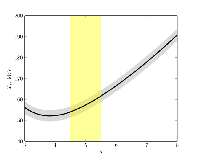
Figure 1: The chiral crossover temperature $T_{\chi}$ as a function of the Yukawa coupling, $y$. In the horizontal shaded region $T_{d}$ varies from $260$ to $280$ MeV, with the line $T_{d}=270$ MeV. The vertical shaded region corresponds to $y:4.5\rightarrow 5.5$.

Given the range in the Yukawa coupling, we can then determine the masses of the $0^{+}$ mesons at zero temperature. In Table (1) we show the values of the $a_{0}$, $f_{0}$, and $\sigma$, for values of $y=4.5$, $5$, and $5.5$.

The variation of the mass of the $a_{0}$ at $T=0$, as a function of the Yukawa coupling, is shown in Fig. (2).

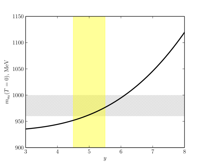
Figure 2: The mass of $a_{0}$ meson at zero temperature as a function of the Yukawa coupling, $y$. The horizontal shaded region corresponds to the experimental uncertainty in the $a_{0}$ mass.

The mass of the $a_{0}$ in all cases is near the experimental value of $980$ MeV, although low by $\sim 3\%$. The mass of the $f_{0}$ is a bit below $1$ GeV, while the $\sigma$ is very low, $\sim 325$ MeV. These values are typical of linear sigma models Lenaghan et al. (2000).

$y$	$m_{a_{0}}$	$m_{f_{0}}$	$m_{\sigma}$
4.5	952	982	309
5	962	966	328
5.5	977	945	348

Table 1: Meson masses as functions of the Yukawa coupling.

We choose the central value of “$y=5$”. The properties of the theory at $\mu=0$ then follow directly.

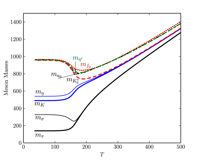
Figure 3: Temperature dependence of the meson masses for $y=5$.

The temperature dependence of the meson masses at nonzero temperature are shown in Fig. (3). Above $T\sim 200$ MeV, we find that the following masses are degenerate: the $\pi$ and $\sigma$; the $K$, $\eta$, and $K_{0}^{*}$; and the $a_{0}$, $f_{0}$, and $\eta^{\prime}$. This is expected for the restoration of the $SU(3)_{L}\times SU(3)_{R}$ chiral symmetry, with the small mass splittings due to the residual symmetry breaking from $m_{u}=m_{d}\ll m_{s}\neq 0$.

Notice that the mass spectrum does not exhibit the restoration of the axial $U(1)_{A}$ symmetry, as the $\eta^{\prime}$ meson is heavier than the $\eta$ meson. This is because we assume that the coefficient $c_{A}$ is fixed, and does not vary with temperature. This is clearly unphysical, as seen in lattice simulations Buchoff et al. (2014), and as we discuss in Sec. (V.6).

V.3 Thermodynamics

Turning to thermodynamics, the pressure is illustrated in Fig. (4). The agreement with the pressure is reasonable, but not spectacular. The pressure in the chiral matrix model is too small at low temperature, below $T_{\chi}$. This is because we do not include light hadrons such as pions, kaons, etc. as dynamical degrees of freedom.

At high temperature, above $250$ MeV, the pressure in our model overshoots that from the lattice data. This is because we choose the parameters in the gluon potential to be identical to those in the pure glue theory. A better fit could be obtained if we allowed this potential to vary.

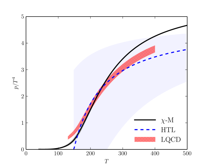
Figure 4: The pressure as a function of temperature. The solid black line is our chiral matrix model, $\chi$-M. The shaded region about this denotes the variation of the Yukawa coupling, $y:4.5\rightarrow 5.5$. The red band are the results from lattice simulations Bazavov et al. (2014). The dashed blue line is that of NNLO HTL perturbation theory, with the band changing the renormalization mass scale by a factor of two Andersen et al. (2010a); *andersen_gluon_2010; *andersen_nnlo_2011; *andersen_three-loop_2011; *haque_two-loop_2013; *mogliacci_equation_2013; *haque_three-loop_2014.

To see the discrepancy with the lattice results, in Fig. (5) we show the interaction measure, $(e-3p)/T^{4}$, where $e(T)$ is the energy density. This peak in the interaction measure is about $25\%$ too high: it is $\sim 5$, versus $\sim 4$ from the lattice. Also, the peak in the interaction measure is at $\sim 220$ MeV, versus $\sim 200$ MeV from the lattice.

Figure 5: The interaction measure as a function of $T$. The black line denotes the chiral matrix model, $\chi$-M, with the shaded band the variation in $y:4.5\rightarrow 5.5$. The red band are the results from lattice simulations Bazavov et al. (2014). The dashed blue line is that of NNLO HTL perturbation theory, with the band changing the renormalization mass scale by a factor of two Andersen et al. (2010a); *andersen_gluon_2010; *andersen_nnlo_2011; *andersen_three-loop_2011; *haque_two-loop_2013; *mogliacci_equation_2013; *haque_three-loop_2014.

V.4 Behavior of the order parameters

How the order parameters change with temperature is illustrated in Fig. (6). We show the Polyakov loop directly, while for the chiral order parameters, we show the ratio of the condensate at $T\neq 0$ to that at $T=0$. This figure shows that in our matrix model there is an extremely close correlation between the restoration of chiral symmetry, and deconfinement, as the decline in the light quark condensate mimics the rise in the Polyakov loop, for temperatures between $100$ and $300$ MeV. To be more precise, one can compute the associated susceptibilities for the order parameters. We defer this to Sec. (V.4), so that we can discuss at length which susceptibilities diverge in the chiral limit. As expected for a heavy quark, the strange quark condensate declines much slower than that for the light quarks.

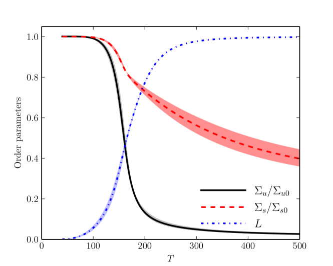
Figure 6: The chiral and deconfining order parameters as functions of $T$. The light and strange chiral condensates are normalized to their value at zero temperature. The shaded regions correspond to varying the Yukawa coupling $y$ in the range $y:4.5\rightarrow 5.5$.

The chiral order parameters cannot be directly compared to those on the lattice. Even their mass dimensions are different: in our model $\Sigma$ has dimensions of mass, while in QCD $\langle\overline{\psi}\psi\rangle$ has dimensions of mass³.

Further, in QCD the quark condensate has a quadratic ultraviolet divergence. Analytically we can eliminate this divergence by using dimensional regularization, but on the lattice, there are terms $\sim 1/a^{2}$, where $a$ is the lattice spacing. In numerical simulations, this divergence is eliminated by computing the difference between the condensates between the light and heavy quarks, weighted by the quark mass difference:

$$\Delta_{u,s}^{lattice}(T)=\frac{\langle\overline{\psi}\psi\rangle_{u,T}-(m_{u}/m_{s})\langle\overline{\psi}\psi\rangle_{s,T}}{\langle\overline{\psi}\psi\rangle_{u,0}-(m_{u}/m_{s})\langle\overline{\psi}\psi\rangle_{s,0}}\;.$$ (109)

Here $m_{u}$ and $m_{s}$ are the current quark masses for the up and strange quarks, and $\langle\overline{\psi}\psi\rangle$ the corresponding condensates.

We then compute this ratio of condensates in our model, where the analogous quantity is

$$\Delta_{u,s}^{\chi-M}(T)=\frac{\Sigma_{u}(T)-(h_{u}/h_{s})\Sigma_{s}(T)}{\Sigma_{u}(0)-(h_{u}/h_{s})\Sigma_{s}(0)}\;.$$ (110)

These two quantities are shown in Fig. (7). The close agreement between the lattice results of Ref. Bazavov et al. (2012a) and the matrix model is satisfying.

Figure 7: The subtracted chiral condensates, from the lattice Bazavov et al. (2012a), Eq. (109), and the matrix model, Eq. (110).

In contrast, there is a strong difference in the value of Polyakov loop in our model, and from the lattice Bazavov and Petreczky (2013); Bazavov et al. (2016). This is illustrated in Fig. (8). The Polyakov loop in the matrix model approaches unity much quicker than measurements of the (renormalized) Polyakov loop on the lattice.

Given the good qualitative agreement between the susceptibilities in the model and the lattice, this disagreement for the Polyakov loop must be considered the outstanding puzzle of our model. We note that a similar disagreement was seen in the pure gauge theory Dumitru et al. (2011, 2012). For this reason, in Sec. (VII) we consider alternate models in which we fit the Polyakov loop, more or less by hand. We show that doing so obviates any agreement for other quantities, such as the pressure and susceptibilities.

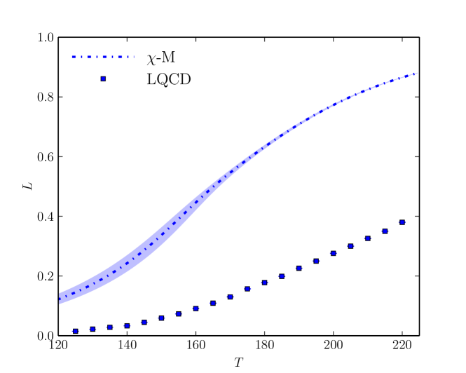
Figure 8: The Polyakov loop in the matrix model and from the lattice Bazavov and Petreczky (2013); Bazavov et al. (2016). The band in the matrix model corresponds to the variation in the Yukawa coupling from $y:4.5\rightarrow 5.5$, as shown before.

V.5 Susceptibilities for the order parameters, and their divergences in the chiral limit

To better understand how the chiral and deconfining order parameters are related, it is useful to compute their associated susceptibilities. This is shown in Fig. (9). These are normalized to be dimensionless quantities by multiplying by the relevant powers of $T_{\chi}$, except for those for the loop-loop and loop-antiloop, where we use $T^{2}T_{\chi}^{2}$.

As expected, the largest peak is that for the light quark condensate, $\Sigma_{u}-\Sigma_{u}$. That for $\Sigma_{u}-\Sigma_{s}$ is less sharp, and even more so for $\Sigma_{s}-\Sigma_{s}$. This is unremarkable, demonstrating that a heavy quark is farther from the chiral limit than light quarks.

The susceptibility for the loop correlations are broad. For both the loop-loop and loop-antiloop correlations, they peak about $T_{\chi}$, with a wide width, due to their coupling to the light quark fields.

The susceptibilities of the loop-antiloop have been computed on the lattice by Bazavov et al. Bazavov et al. (2016). Their results peak at a significantly higher temperature than we find in the chiral matrix model, at $\sim 200$ MeV. This presumably is due to the fact that the lattice Polyakov loop is shifted to higher temperatures than in the chiral matrix model. They did not investigate the susceptibility between the loop and the chiral order parameter.

Returning to our results, after the $\Sigma_{u}-\Sigma_{u}$ correlation, the sharpest peak is for that between the loop and the light quark condensate, $\Sigma_{u}-\ell$. This is not an artifact. In a Polyakov loop model, Sasaki, Friman, and Redlich Sasaki et al. (2007) found that the $\Sigma$-loop correlation is divergent: see Fig. (19) of Ref. Sasaki et al. (2007).

This is a general result for a chiral transition of second order. To show this, we consider the interaction of the lowest mass dimension between a chiral field $\Phi$ and the Polyakov loop $\ell$,

$$\left(\ell+\ell^{*}\right){\rm tr}\left(\Phi^{\dagger}\Phi\right)\;.$$ (111)

This coupling respects all of the relevant symmetries of gauge invariance and chiral symmetry. It is not invariant under the global color symmetry of $Z(3)$, but since this symmetry of the pure gauge theory is violated by the presence of dynamical quarks, it does arise. In particular, such a coupling appears in our chiral matrix model. In general, and in the chiral matrix model, there is an infinite series of Polyakov loops, in different representations, which couple to ${\rm tr}\Phi^{\dagger}\Phi$. We shall argue that this does not alter our conclusions about the critical behavior which follow.

Consider the mass matrix between the chiral field and the Polyakov loop. We can concentrate on the field $\Sigma$ which is nonzero in the phase with chiral symmetry breaking. The mass squared matrix between $\Sigma$ and $\ell$ is

$${\cal M}^{2}=\left(\begin{array}[]{cc}m^{2}&\kappa\,\Sigma_{f}\\ \kappa\,\Sigma_{f}&\widetilde{m}^{2}\\ \end{array}\right)\;,$$ (112)

where $\kappa$ is some constant, and $\widetilde{m}^{2}$ the mass for the loop. Assuming the chiral transition is of second order,

$$m^{2}\sim\delta t\;\;\;;\;\;\;\Sigma_{f}\sim\delta t^{\beta}\;\;\;;\;\;\;\delta t\equiv\left|\frac{T-T_{\chi}}{T_{\chi}}\right|\;.$$ (113)

That the mass of the $\Sigma$ field vanishes as the reduced temperature $\delta t$ is standard. Similarly, the expectation value of $\Sigma$ vanishes with critical exponent $\beta$. The mass of the Polyakov loop is assumed to be nonzero at the chiral phase transition, since it is not a critical field.

The susceptibilities are determined by the inverse of this matrix. Consequently, for that between the loop and the condensate, we obtain

$$\left.\frac{1}{{\cal M}^{2}}\right|_{\ell\,\Sigma}\sim\delta t^{\beta-1}\;.$$ (114)

In this we assume that $\beta<1/2$, which is true for the $O(4)$ universality class, which is what enters for two massless flavors Pisarski and Wilczek (1984).

It is direct to show that Eq. (114) is true in a chiral matrix model. In such a model the coupling is not between the loop $\ell$ and the scalar field, but between $q$ and $\Phi$. What matters is that in the phase with $\Sigma_{f}\neq 0$, there is a coupling between $q$ and $\Phi$ which is $\sim\Sigma_{f}$. This factor can be understood as follows. The loop diagram between a $q$ field and the $\Sigma$ is proportional to

$${\rm tr}\;\gamma^{0}\;\lambda_{3}\;\frac{1}{(/\!\!\!\!D^{bk}+m_{f})^{2}}$$ (115)

The factor of $\gamma^{0}$ is from the coupling to $q$, while the coupling of a quark antiquark to $\Sigma$ is proportional to unity. This diagram is nonzero only if the Dirac trace is over two Dirac matrices, so one of the propagators must bring in a factor of the quark mass, $m_{f}\sim y\Sigma_{f}$. The mixed susceptibility between the loop and $q$ then behaves as $\sim y\Sigma_{f}/m^{2}\sim 1/\delta t^{1/2}$. This is the expected behavior in mean field theory, where $\beta=1/2$.

Viewed in a general context of second order phase transitions, it is not surprising that the coupling between a critical field $\Phi$, and a noncritical field, $\ell$, gives a weak but divergent susceptibility for the off-diagonal susceptibility between $\Phi$ and $\ell$. Indeed, assuming that the expectation value of the loop is nonzero at $T_{\chi}$, even $Z(3)$ symmetric operators such as $|\ell|^{2}{\rm tr}\Phi^{\dagger}\Phi$ would produce a divergent susceptibility. However, they would be smaller by powers of the expectation value of the loop, which is small in QCD at $T_{\chi}$.

Figure 9: The susceptibilities for the chiral and deconfining order parameters, as a function of the temperature $T$.

V.6 Chiral susceptibilities and $U(1)_{A}$

In Fig. (3) we showed the meson masses as a function of temperature. As discussed at the end of Sec. (V.2), it still exhibits a violation of the axial $U(1)_{A}$, with the mass of the $\eta^{\prime}$ meson heavier than that of the $\eta$ meson.

This splitting is controlled by the coefficient $c_{A}$ in the effective Lagrangian. Dynamically, at high temperature $c_{A}$ should decrease with temperature, as instanton fluctuations are suppressed by the Debye mass Gross et al. (1981).

To study the restoration of the axial $U(1)_{A}$ symmetry, numerical simulations have studied chiral susceptibilities which are sensitive to this breaking Buchoff et al. (2014). In a chirally symmetric phase, the susceptibilities for the $\sigma$ and $\pi$ are equal, as are those for the $\eta^{\prime}$ and the $a_{0}$. This degeneracy is demonstrated by the meson masses in Fig. (3). That the $\pi$ and $a_{0}$ masses are unequal is manifestly due to $c_{A}\neq 0$. Neglecting the temperature dependent symmetry breaking term, this is clear from the expressions for these masses in Eqs. (68) and (77): with $\Sigma_{u}\approx 0$, $m_{\pi}^{2}=m^{2}-c_{A}\,\Sigma_{s}$ and $m_{a_{0}}^{2}=m^{2}+c_{A}\,\Sigma_{s}$.

Numerical simulations find that while the $\pi$ and $a_{0}$ susceptibilities differ at $T_{\chi}\sim 155$ MeV, they are essentially equal by $T_{U(1)_{A}}\sim 200$ MeV. At zero temperature there is a close relationship between the spontaneous breaking of chiral symmetry and anomalous amplitudes, such as for $\pi^{0}\rightarrow\gamma\gamma$. Naively this suggests that $T_{U(1)_{A}}\approx T_{\chi}$. However, at nonzero temperature Lorentz invariance is lost, and this relationship is much more involved Pisarski et al. (1997). Consequently, the two temperatures $T_{U(1)_{A}}$ and $T_{\chi}$ can differ. The lattice shows that $T_{U(1)_{A}}>T_{\chi}$; for other numbers of flavors and colors, to us it seems possible that $T_{U(1)_{A}}<T_{\chi}$.

One might hope to compute the $\pi$ and $a_{0}$ susceptibilities in the matrix model, to fix the temperature dependence of $c_{A}$. This was done in Ref. Ishii et al. (2016) in a Polyakov Nambu-Jona-Lasino model.

The difficulty is that while our chiral matrix model can be used to compute many quantities, it cannot be used to compute all. Consider the quark operator with pion quantum numbers, $J_{5}^{a}=\overline{\psi}\tau^{a}\gamma_{5}\psi$. The chiral susceptibility for the pion is dominated by single pion exchange, $\sim\langle 0|J_{\pi}|\pi\rangle 1/m_{\pi}^{2}\langle\pi|J_{\pi}|0\rangle$.

The form factors are determined by partially conserved axial current. The axial current satisfies $\partial_{\mu}J_{\mu}^{5,a}=2m_{qk}J_{5}^{a}$, where $J_{\mu}^{5,a}=\overline{\psi}\tau^{a}\gamma_{\mu}\gamma_{5}\psi$, and $m_{qk}$ is the current quark mass. Since $\langle 0|J_{\mu}^{5,a}|\pi\rangle\sim P^{\mu}f_{\pi}$, using $P^{2}=m_{\pi}^{2}=m_{qk}\langle\overline{\psi}\psi\rangle/f_{\pi}^{2}$, we find that $\langle\pi|J_{\pi}|0\rangle\sim\langle\overline{\psi}\psi\rangle/f_{\pi}$.

In QCD, the expectation value is $\langle\overline{\psi}\psi\rangle\sim-(300~{}MeV)^{3}$. In the chiral matrix model, computation shows that the analogous quantity is much smaller, $\langle\overline{\psi}\psi\rangle\sim-m_{\pi}^{3}\sim-(140~{}MeV)^{3}$. This difference is consistent with chiral symmetry: in QCD the condensate only enters multiplied by the current quark mass. In the chiral matrix model, the pion mass is related to the background field $h_{u}$, and has no direct relation to the chiral condensate $\langle\overline{\psi}\psi\rangle$.

However, what matters for the associated chiral susceptibilities are the form factors, and so $\langle\overline{\psi}\psi\rangle$. These are too small by an order of magnitude, and so cannot be used to constrain $c_{A}$.

VI Flavor susceptibilities

Besides the computation of bulk thermodynamic properties, most useful insight is gained by computing derivatives with respect to quark chemical potentials.

In principle this is straightforward, simply the derivative of the effective potential with respect to the relevant $\mu$, evaluated at $\mu=0$. For example, the baryon number susceptibility is given by

$$\chi_{n}^{B}=T^{n-4}\;\left.\frac{\partial^{n}P}{\partial\mu_{B}^{n}}\right|_{\mu=0}\;.$$ (116)

Particularly in our model, it is trivial to take derivatives with respect to a given flavor, to compute the corresponding susceptibility.

At the outset we should note that because we treat the mesons in mean field approximation, implicitly we neglect fluctuations from pions. Pion fluctuations are not important in computing susceptibilities with respect to baryon number and strangeness, but do matter in computing those with respect to other chemical potentials, including those for up and down flavor number, isospin, and charge.

There is one point which must be treated with care, as was discussed in Sec. (III.2). Most quantities are even under charge conjugation, ${\cal C}$. This includes the effective potential, and the stationary points for the chiral condensates, $\Sigma_{u}$ and $\Sigma_{d}$, and for the Polyakov loop, $q$. The latter is not obvious: while the gauge potential $A_{0}\rightarrow-A_{0}^{*}$ under ${\cal C}$, because we assume that the stationary point for the Polyakov loop is real, we always sum over $q$ and $-q$. That these quantities are even under ${\cal C}$ greatly simplifies how they can enter into quark number susceptibilities.

Previously, however, we argued that when $\mu\neq 0$, that the stationary point involves imaginary values of $r=i{\cal R}$, Eq. (42). This means that we can compute quark number susceptibilities using a type of Furry’s theorem: loops with insertions of $\mu$ correspond to a type of coupling to an Abelian gauge field. There must be an even number of insertions, where both insertions of $\mu$ or $r$ can enter. Since we work in mean field approximation, only one field can be exchanged.

VI.1 Second order susceptibilities

Let us start with the simplest quantity, $\chi_{2}^{B}$. The diagrams which contribute are illustrated in Fig. (10). The first diagram, on the left, is expected: two insertions of the chemical potential into a quark loop. What is unexpected is the second diagram, where one has two quark loops, each with single insertions of $\mu$ and $r$, coupled by a single propagator for $r$. Since we are computing fluctuations, that the stationary point in $r$ is imaginary is really secondary; what matters is that $r$, like $\mu$, is ${\cal C}$ odd. Thus both diagrams satisfy Furry’s theorem. Note that the second diagram is only nonzero when $q\neq 0$: otherwise, as an insertion of $r$ brings in $\lambda_{8}$, Eq. (25), the color trace vanishes.

Figure 10: Contributions to the second order baryon number susceptibility $\chi_{2}^{B}$: (a) the one particle irreducible and (b) the one particle reducible. The wiggly line denotes $r-r$ propagator.

The results for $\chi_{2}$ are given in Fig. (11). It is completely dominated over all temperatures by the one particle irreducible contribution in Fig. (10a). The second diagram, from the exchange of a $r$ gluon, is present, but numerically small over all temperatures.

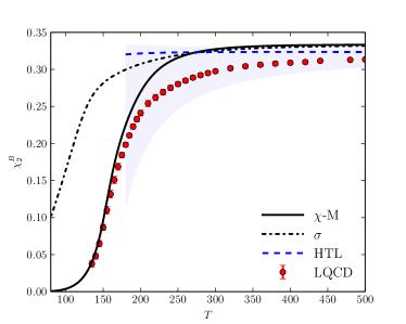
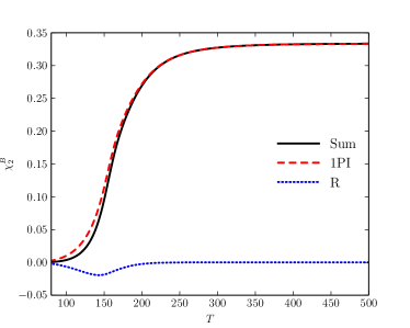
Figure 11: The second order baryon number susceptibility as a function of the temperature. The left panel shows the results in the chiral matrix ($\chi-M$) model, compared to a $\sigma$ model, HTL resummation Andersen et al. (2010a); *andersen_gluon_2010; *andersen_nnlo_2011; *andersen_three-loop_2011; *haque_two-loop_2013; *mogliacci_equation_2013; *haque_three-loop_2014, and numerical simulations on the lattice. The right panel shows contributions to the chiral matrix model: it is dominated by the contribution of the one particle irreducible contribution, Fig. (10a), over $r$-exchange in Fig. (10b).

The results of the chiral matrix ($\chi-M$) model approach the asymptotic value of $1/3$ faster than the lattice data. However, the gross behavior agrees with the lattice. The chiral matrix model certainly agrees much better with the lattice data than Hard Thermal Loop resummation, which stays near $1/3$. More surprisingly, it also agrees much better than a sigma model, which incorporates chiral symmetry breaking, but not the nontrivial holonomy of the Polyakov loop, $q\neq 0$. We shall see this is true for higher susceptibilities as well.

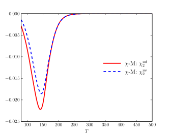
Figure 12: The second order off-diagonal susceptibilities as a function of the temperature.

One can also compute the off-diagonal susceptibilities. Those for light-light, $ud$, and heavy-light, $us$, are illustrated in Fig. (12). This is a very interesting quantity to compute, because on the lattice, it is due to disconnected diagrams. In our model, the off-diagonal susceptibilities are due entirely not to the connected diagram, Fig. (10.a), but to the diagram from the exchange of an $r$ gluon, Fig. (10.b).

In our model, we find that the off-diagonal susceptibilities for $ud$ and $us$ are nearly equal. This is easy to understand, because the difference is only one of form factors: generating an $r$ gluon from an up loop is about as probable as from a strange loop.

The results of our model for the off-diagonal susceptibilities $us$ are in reasonable agreement with lattice simulations. On the other hand, the results for $ud$ are about an order of magnitude smaller than measured on the lattice. This is because we do not include dynamical hadrons, in particular pions, in our model. The most direct way of including dynamical pions would be to use the Functional Renormalization Group Skokov et al. (2012).

VI.2 Fourth order susceptibilities

Turning to the fourth order susceptibility, the diagrams which contribute are those of Fig. (13). The diagrams include four insertions of the chemical potential into a quark loop, Fig. (13.a). Then there are two insertions of the chemical potential into two different loops, connected by the exchange of ${\cal C}$ even fields, either $q$, $\Sigma_{u}$, or $\Sigma_{s}$, Fig. (13.b). Lastly, there is diagram from one quark loop, with a single insertion of $\mu$, and another quark loop, with three insertions of $\mu$, connected by the exchange of an $r$ gluon.

Figure 13: Contributions to the fourth order baryon number susceptibility $\chi_{4}^{B}$: (a) the one particle irreducible and (b-c) the one particle reducible. Only diagrams to two quark loop order are shown, which are not inclusive. The dashed line denotes the propagator for ${\cal C}$ even fields, $q$, $\Sigma_{u}$, and $\Sigma_{s}$; the gluon line, for $r$.

The results for the fourth order baryon number susceptibility are shown in Fig. (14). In this case, the one particle irreducible contribution of Fig. (13.a) gives a smooth contribution which is no longer dominant. Instead, the exchange of a $q$ gluon gives the largest contribution near $T_{\chi}$. Indeed, this is larger than that of the $\Sigma_{u}$ field.

The results of the chiral matrix model for $\chi_{4}^{B}$ appear to overshoot the results of the lattice by a factor of two near $T_{\chi}$, but the lattice results have large error bars. More striking is that the Hard Thermal Loop result is essentially constant with respect to temperature, while a sigma model gives a result which is too small, and peaked at a temperature significantly below that of the lattice data.

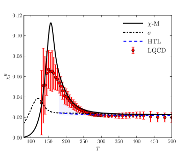
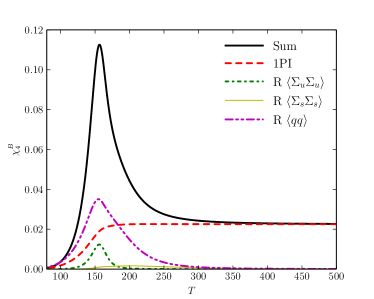
Figure 14: The fourth order baryon number susceptibility as a function of the temperature. The left panel shows the results in the chiral matrix ($\chi-M$) model, compared to a $\sigma$ model, HTL resummation Andersen et al. (2010a); *andersen_gluon_2010; *andersen_nnlo_2011; *andersen_three-loop_2011; *haque_two-loop_2013; *mogliacci_equation_2013; *haque_three-loop_2014, and numerical simulations on the lattice. The right panel shows contributions to the chiral matrix model; only those from Fig. (13) are shown, which are not inclusive.

It is also interesting to plot the difference of the second and fourth order baryon susceptibilities.

Consider the contribution of the quarks to the pressure for a single flavor,

$$p=-\,2\,T\,\sum_{a=1}^{N_{c}}\int\frac{d^{3}k}{(2\pi)^{3}}\ln\left(1+e^{-E_{f}/T-\mu/T+i\frac{2\pi}{3}q_{a}}\right)+\ln\left(1+e^{-E_{f}/T+\mu/T-i\frac{2\pi}{3}q_{a}}\right).$$ (117)

Expanding in powers of the fugacity,

$$p=\frac{m^{2}T^{2}N_{c}}{\pi^{2}}\sum_{n=1}^{\infty}\frac{(-1)^{n+1}}{n^{2}}K_{2}(nm/T)\left(\ell_{n}e^{n\mu/T}+\ell^{\dagger}_{n}e^{-n\mu/T}\right)$$ (118)

where $\ell_{n}$ is the Polyakov loop in the fundamental representation which wraps around in imaginary time $n$ times,

$$\ell_{n}=\frac{1}{N_{c}}\sum_{a=1}^{N_{c}}\exp\left(i\frac{2\pi}{3}q_{a}\right).$$ (119)

The $\ell_{n}$ can be expressed in terms of loops in various irreducible representations. We shall not need the detailed form. All that matters here is that those which wrap around a multiple of $N_{c}$ times include the identity representation. At small temperatures, these terms are nonzero, and so dominate.

To eliminate the contribution of such “baryonic” loops, we construct a quantity for which $\ell_{N_{c}}$ cancels. Notice that to second and fourth order, the baryon number susceptibilities are

$$\chi_{2}^{B} = \frac{2\,N_{c}\,m^{2}}{9\,\pi^{2}\,T^{2}}\sum_{n=1}^{\infty}(-1)^{n+1}K_{2}\left(\frac{nm}{T}\right)\;\ell_{n}\;,$$ (120)

$$\chi_{4}^{B} = \frac{2\,N_{c}\,m^{2}}{81\,\pi^{2}\,T^{2}}\sum_{n=1}^{\infty}(-1)^{n+1}n^{2}K_{2}\left(\frac{nm}{T}\right)\;\ell_{n}\;.$$ (121)

For three colors the difference between the two is

$$\chi_{2}^{B}-\chi_{4}^{B}\approx\frac{2\,m^{2}}{27\,\pi^{2}\,T^{2}}\left(8K_{2}\left(\frac{m}{T}\right)\;\ell_{1}-5K_{2}\left(\frac{2m}{T}\right)\ell_{2}+\ldots\right)\;.$$ (122)

The contribution from the loop $\ell_{3}$ cancels in the difference. One can show that $\ell_{2}=\ell_{1}(3\,\ell_{1}-2)$, so at small temperature, $\chi_{2}^{B}-\chi_{4}^{B}$ is proportional to the loop, $\ell_{1}$. There are also terms $\sim\ell_{4},\ell_{5}$ and so on in Eq. (122), but these are numerically small.

In Fig. (15) we plot this difference as a function of the temperature. The chiral matrix model agrees very well with the lattice results up to temperatures of $\sim 200$ MeV, and then goes more quickly to a constant value than the lattice data. In contrast, HTL resummation gives essentially a constant value Andersen et al. (2010a); *andersen_gluon_2010; *andersen_nnlo_2011; *andersen_three-loop_2011; *haque_two-loop_2013; *mogliacci_equation_2013; *haque_three-loop_2014. More surprising, a sigma model, which includes chiral symmetry restoration but not the change in the Polyakov loop, is much higher than the lattice data. As can be seen from the panel on the right-hand side, this difference of susceptibilities is nearly proportional to the Polyakov loop.

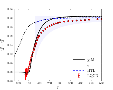
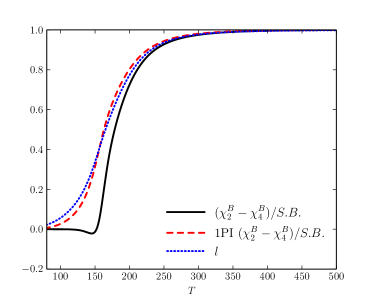
Figure 15: The difference between the second and forth order baryon number susceptibilities as a function of the temperature.

VI.3 Sixth order susceptibilities

We conclude with results for the sixth order baryon susceptibility. Some of the diagrams which contribute are illustrated in Fig. (16). We only show the diagrams with up to two quark loops. We note, however, that the diagrammatic method is not particularly useful for computing the susceptibilities. Instead, direct numerical evaluation was used.

Figure 16: Contributions to the sixth order baryon number susceptibility $\chi_{6}^{B}$: (a) the one particle irreducible and (b-d) the one particle reducible. Only diagrams with two quark loops and less are shown. Diagrams up to two quark loops are shown only. The dashed line denotes the propagator of $\vec{\phi}=(q,\Sigma_{u},\Sigma_{s})$. The propagator has off-diagonal elements.

The results are shown in Fig. (17). There are preliminary results available on the lattice, but none are continuum extrapolated, and so we do not show these. The results of HTL resummation are very small Andersen et al. (2010a); *andersen_gluon_2010; *andersen_nnlo_2011; *andersen_three-loop_2011; *haque_two-loop_2013; *mogliacci_equation_2013; *haque_three-loop_2014. This is expected: in perturbation theory the pressure is $\mu^{4}$ times a power series in the coupling constant. Thus contributions to $\chi_{6}^{B}$ are suppressed at least by powers of $g^{2}$.

What is not evident is not in contrast to a $\sigma$ model, the chiral matrix model shows a strong nonmonotonic behavior, with a large amplitude of oscillation. The $\sigma$ model behaves similarly, but occurs below $T_{\chi}$, and is almost an order of magnitude smaller than the chiral matrix model.

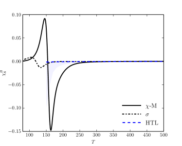
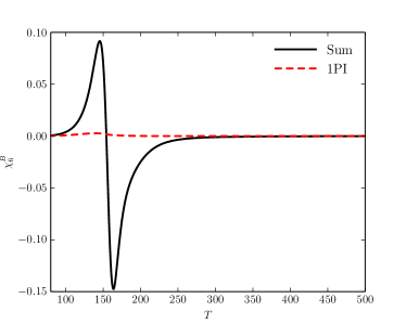
Figure 17: The sixth order baryon number susceptibility as a function of the temperature, in the chiral matrix model ($\chi-M$), a sigma model, and HTL resummation Andersen et al. (2010a); *andersen_gluon_2010; *andersen_nnlo_2011; *andersen_three-loop_2011; *haque_two-loop_2013; *mogliacci_equation_2013; *haque_three-loop_2014.

VII Alternate models

The principle problem with the chiral matrix model is that while most quantities agree well with lattice results, that for the Polyakov loop, Fig. (8), does not.

Consequently, in this section we consider alternate models, where we fix the value of the Polyakov loop to agree with the results from numerical simulations. We then compute various quantities, and consider if the agreement is better or worse than with our original model. In all cases, we find that the agreement is worse. We discuss this further in the Conclusions, Sec. (VIII).

VII.1 Pure gauge theory

We start with the theory without dynamical quarks. In Sec. (III) we took the nonperturbative gluon potential from Refs. Dumitru et al. (2011, 2012), where it is assumed that the only terms are even powers of temperature, $\sim T^{4}$, $T^{2}$, and $T^{0}$. The simplest generalization is then to assume arbitrary powers of temperature.

In order to fit the Polyakov loop, we use an observation of Megias, Ruiz Arriola, and Salcedo Megias et al. (2007). They showed that except close to $T_{d}$, the expectation value of the Polyakov loop is close to an exponential in $1/T^{2}$, $\langle\ell\rangle\sim{\rm e}^{-\#T_{d}^{2}/T^{2}}$. Numerical simulations by Gupta, Hübner, and Kaczmarek show this holds for both three colors Gupta et al. (2008); Mykkanen, Panero, and Rummukainen show it is valid for two to six colors Mykkanen et al. (2012). At large $T$, then, $\langle\ell\rangle-1\sim 1/T^{2}$. While a matrix model will not give an exponential behavior of the Polyakov loop in any natural way, at least at large $T$ this parametrization indicates that $\langle q\rangle\sim 1/T$.

The perturbative gluon potential is fixed by perturbation theory to be that of Eq. (29). For $r=0$, this potential involves

$${\cal V}_{4}(q,0)\equiv{\cal V}_{4}(q)=\frac{2}{3}\,q^{2}\,\left(1-\frac{10}{9}\,q+\frac{1}{3}\,q^{2}\right)\;.$$ (123)

We assume that we use the same kind of functions as before, Eq. (33). Thus we also need

$${\cal V}_{2}(q,0)\equiv{\cal V}_{2}(q)=\frac{2}{3}\,q\,\left(2-q\right)\;.$$ (124)

We then generalize the potential of Eq. (33) by assuming that the coefficients of these functions involves not just $T^{2}$, but arbitrary powers of temperature, $T^{3}$, $T^{2}$, and $T$:

$${\cal V}_{non}^{gl}(q)=\frac{4\pi^{2}}{3}\;T_{d}^{4}\left(\left(\alpha\,t^{3}+\beta\,t^{2}+\gamma\,t\right){\cal V}_{2}(q)+\left(\alpha^{\prime}\,t^{3}+\beta^{\prime}\,t^{2}+\gamma^{\prime}\,t\right){\cal V}_{4}(q)+\frac{2}{15}c_{3}\,t^{2}\right)\;,$$ (125)

where

$$t=\frac{T}{T_{d}}\;.$$ (126)

Consider the behavior of this model at high temperature, where $q$ is small. The dominant behavior is given by balancing the perturbative potential, $\sim T^{4}{\cal V}_{4}\sim T^{4}q^{2}$, against the nonperturbative term, $\sim T^{3}{\cal V}_{2}\sim T^{3}q$. This gives $\langle q\rangle\sim 1/T$ at large $T$, which as we discussed above is suggested by measurements of the renormalized Polyakov loop.

Following Refs. Dumitru et al. (2011, 2012), we impose two conditions. The first is that the pressure (approximately) vanishes at the critical temperature. This can be used to determine the constant term, $\sim c_{3}$:

$$c_{3}=\frac{1}{27}\left(47-20\alpha^{\prime}-20\beta^{\prime}-20\gamma^{\prime}\right)\;.$$ (127)

The second condition is given by requiring that the transition occurs at $T_{d}$.

The previous potential, Eq. (33), starts with three coefficients, which then reduce to one free parameter. The new model begins with seven parameters, which reduce to five free parameters. By some trial and error, we are led to the values

$$\alpha=-0.403376\;;\;\alpha^{\prime}=-1.00819\;;\;\beta=-2.58495\;;\;$$

$$\beta^{\prime}=-8.6023\;;\;\gamma=1.12179\;;\;\gamma^{\prime}=5.57084\;.$$ (128)

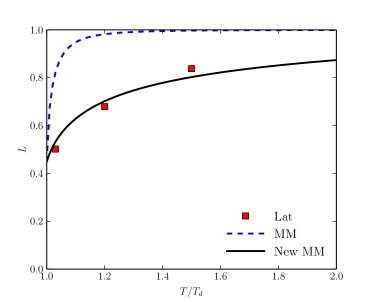
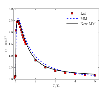
Figure 18: Results from the previous matrix model (MM), Eq. (33), and in the new matrix model (New MM), Eqs. (125) and (128). With five free parameters in the New MM, as opposed to one in the MM, good fits for both the Polyakov loop, in the left panel, and for the interaction measure, $(e-3p)/T^{4}$, in the right panel, can be obtained.

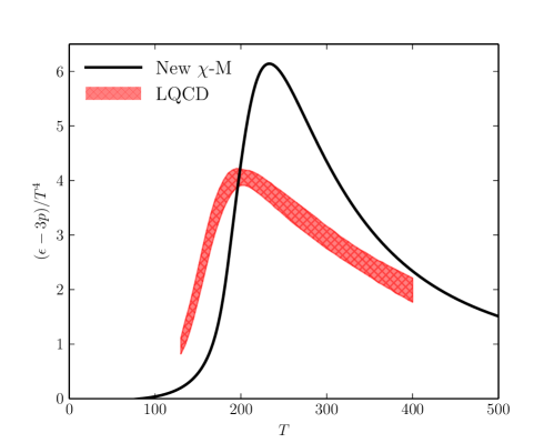
Figure 19: Results for $(e-3p)/T^{4}$ for the new matrix model, Eqs. (125) and (128), with dynamical quarks. The result is farther from the lattice values than our original model, see Fig. (5).

The results for the Polyakov loop and the interaction measure, $(e-3p)/T^{4}$, are shown in Fig. (19). Given the plethora of parameters, it is hardly surprising that we can fit both the Polyakov loop and the pressure at all temperatures above $T_{d}$.

We then adopt the same approach as before to include dynamical quarks. The results are shown in Fig. (18). The results are not close to those of the lattice, with the peak in the interaction measure in the new matrix model at a much higher value, $\sim 6$ instead of $\sim 4$, and at a significantly larger temperature, $\sim 250$ MeV instead of $\sim 200$ MeV. This should be compared to the results in our original matrix model, Fig. (5); while these are not perfect, they are far closer than those in the new matrix model of Fig. (19).

As before, the value of the Yukawa coupling is $y=5$, with little sensitivity to varying the Yukawa coupling by $\sim 10\%$. We have also computed the chiral order parameter and the susceptibility for light quarks. This shows that the temperature for the chiral crossover in the new matrix model is $T_{\chi}\sim 186$ MeV, which is significantly higher than the lattice value of $T^{lattice}_{\chi}\sim 155$ MeV.

This shows that for the pressure and the transition temperature, that assuming a model which fits the Polyakov loop in the pure gauge theory gives a worst fit to these quantities in QCD. Needless to say, this is under the assumption that there are no new nonperturbative terms in the gluon potential. We could certainly fit both the pressure and loop in QCD by allowing new nonperturbative terms in the gluon potential which are dependent upon presence of quarks. Since we already have a model with five parameters, fitting the pressure and loop in QCD with even more parameters does not seem particularly noteworthy.

VII.2 The Polyakov loop and baryon susceptibilities

To emphasize the physics, then, in this section we assume that the value of the Polyakov loop is given by the value from the lattice. We show in this section that doing so, there is a large and persistent disagreement with the baryon susceptibilities.

Taking the Polyakov loop from the lattice and computing with our chiral model, we find that the chiral crossover temperature is like that in the previous section, and is too large, $T_{\chi}\sim 191$ MeV. For the time being we ignore this to compute the second order baryon susceptibility, $\chi_{2}^{B}$. Our computation is not complete, because we cannot compute the diagram including “r” exchange, which is the diagram on the right-hand side of Fig. (10). Nevertheless, as seen from the diagram on the right-hand side of Fig. (11), this contribution is generally small, and so we assume it can be neglected.

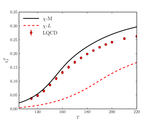
Figure 20: The second order baryon number susceptibility, $\chi_{2}^{B}$, in a model where the Polyakov loop is fitted directly from the lattice, $\chi-L$. This model gives $T_{\chi}\sim 191$ MeV, instead of $T_{\chi}^{lattice}=155$ MeV. Results in our chiral matrix model are shown in $\chi-M$; these are much closer to the lattice data, LQCD.

We present the results in Fig. (20). The overall trend of the results is easy to understand. Because of confinement, $\chi_{2}^{B}$ vanishes in the confined phase, and equals $1/3$ for ideal quarks. Thus being deeper in the confined phase decreases $\chi_{2}^{B}$. This is exactly what is shown in Fig. (20): while the results in our chiral matrix model are slightly higher than those from the lattice, the results with a chiral model which fits the Polyakov loop from the lattice are much lower than the results from $\chi_{2}^{B}$ on the lattice. For example, at $T=200$ MeV, our chiral matrix model is too high by about $\sim 10\%$; in contrast, the value computed from the lattice Polyakov loop is smaller than the lattice $\chi_{2}^{B}$ by about half.

Thus perhaps the problem is that $T_{\chi}$ is too high. Motivated by including the pion degrees of freedom, by hand we adjust the mass squared in the linear sigma model to fit $T_{\chi}$ to be $155$ MeV, as on the lattice. We find that a fit

$$m^{2}\rightarrow m^{2}\left(1+0.1\left(\frac{T}{f_{\pi}}\right)^{2}\right)\;,$$ (129)

suffices: the coefficient of $0.1$ is chosen to obtain $T_{\chi}=155$ MeV.

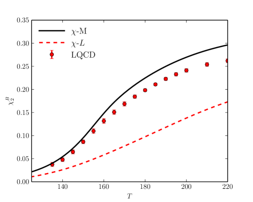
Figure 21: The second order baryon number susceptibility, $\chi_{2}^{B}$, in a model where the Polyakov loop is fitted directly from the lattice, $\chi-L$, and where the mass parameter in the sigma model is tuned by hand, Eq. (129), so that $T_{\chi}=155$ MeV. Results in our chiral matrix model are shown in $\chi-M$; these are much closer to the lattice data, LQCD.

The results in Fig. (21) show that while this approach moves $\chi_{2}^{B}$ upward, closer to the lattice results, it is not by much. As in Fig. (20), fitting to the lattice Polyakov loop gives a result in which $\chi_{2}^{B}$ is rather far from the lattice results.

We have also computed higher order baryon susceptibilities, and find similar results. We also computed using the model of the previous section, and find that the baryon susceptibilities are uniformly farther from the lattice results than in our original chiral matrix model.

We compare our analysis with those of the Functional Renormalization Group (FRG) Braun et al. (2010); Herbst et al. (2011); *fister_confinement_2013; *herbst_phase_2013; *haas_gluon_2014; *herbst_thermodynamics_2014; *mitter_chiral_2015; Herbst et al. (2015); Fu and Pawlowski (2015a, b). In the FRG, the loop approaches unity quickly, as in the chiral matrix model; for the pure gauge theory, see Fig. (1) of Ref. Braun et al. (2010). Herbst, Luecker, and Pawlowski argued that corrections to the FRG modify this so that the loop is much closer to the lattice, Fig. (6) of Ref. Herbst et al. (2015). In QCD, though, Fu and Pawloski computed the baryon susceptibilities Fu and Pawlowski (2015a, b), and find good agreement with the lattice. This requires, however, that the loop is relatively large at $T_{\chi}$: from Fig. (7) of Ref. Fu and Pawlowski (2015b), $\langle\ell\rangle\sim 0.4$ at $T_{\chi}$. This agrees with our conclusions in this section.

VIII Conclusions

The analysis in the previous section shows that the baryon susceptibilities can be a sensitive test of how quickly QCD deconfines.

For light quarks, the baryon susceptibilities are clearly tied to the restoration of chiral symmetry. This suggests that a sensitive test of deconfinement would be to measure the second order baryon susceptibility for a relatively heavy quark. The quark cannot be too heavy, or the entire signal is Boltzmann suppressed. To illustrate this, we show in Fig. (22) $\chi_{2}^{B}$ in our chiral matrix model, versus the results for free, deconfined quarks, with $q=0$. For such a heavy quark, the approximate restoration of chiral symmetry at $T_{\chi}=155$ MeV should not be of relevance. Nevertheless, at this temperature there is a large difference between the two curves, by more than a factor of two.

Thus we suggest that it may be useful to measure $\chi_{2}^{B}$ for a heavy quark in QCD. In the lattice, this heavy quark can be treated in the valence approximation, which should simplify the analysis.

In this vein, we comment on the difference between the second order chiral susceptibilities for light and strange quarks. Bellwied, Szabolcs, Fodor, Katz, and Ratti Bellwied et al. (2013) have described this difference as due to a “flavor hierarchy” between light and strange quarks. In our chiral matrix model, the difference between the two is simply a consequence that because the strange quark is heavier, $\chi_{2}$ tends to lag behind that for a heavier quark. In any case, measuring the susceptibility for a test quark should enable one to disentangle the effects of chiral symmetry restoration versus deconfinement.

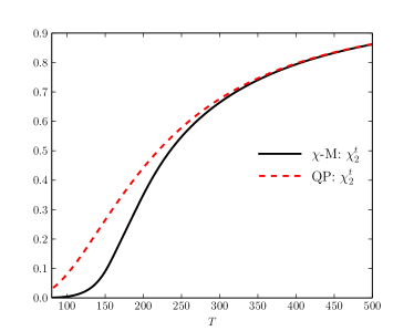
Figure 22: The baryon susceptibility to second order for a heavy test quark, $m=500$ MeV. The solid black line is in our chiral matrix model, the dotted line, for free quarks.

Indeed, one can view the discrepancy between the chiral matrix model and the Polyakov loop more generally. In our model, the approximate restoration of chiral symmetry for light quarks is closely coincident with deconfinement, Fig. (6). Notably, at the chiral crossover temperature, the Polyakov loop is large, $\sim 0.5$. Similarly, the peaks in the susceptibilities for the chiral order parameter for light quarks coincide with the peak for the loop susceptibilities, Fig. (6). Moreover, as demonstrated in Secs. (VI) and (VII), this is also consistent with the baryon susceptibilities, which approach their ideal values rather quickly, certainly by temperatures of $\sim 300$ MeV.

In contrast, the value of the renormalized Polyakov loop Bazavov and Petreczky (2013); Bazavov et al. (2016) from the lattice is extremely small at $T_{\chi}$, $\langle\ell\rangle\sim 0.1$. That is, chiral symmetry is restored in a phase which is nearly confined, not deconfined. If taken at face value, this indicates that even for $\mu=0$, chiral symmetry is restored in a quarkyonic phase McLerran and Pisarski (2007); *andronic_hadron_2010; *kojo_quarkyonic_2010; *kojo_interweaving_2012. Even by temperatures of $200$ MeV, the Polyakov loop is still very small, $\langle\ell\rangle\sim 0.3$. It is hard to understand why the quark susceptibilities are close to their ideal values at relatively low temperatures, $\sim 300$ MeV, if the renormalized Polyakov loop indicates the theory is still close to confining.

We have not settled this question here, but it demonstrates that the thermodynamic behavior of QCD is more involved than naive prejudice might suggest.

Note added. – There is significant overlap between our analysis and that of Kovacs et al. Kovacs et al. (2016), who use a Polyakov loop model coupled to both scalars and vector mesons. While the details of our analyses differ, they also find that the value of the Polyakov loop in their model is much larger than that measured by lattice simulations.

Appendix A Integrals in the semi-QGP

In this appendix we collect some useful integrals.

The trace at zero temperature is defined in Eq. (6). The basic integral for a single massive field is given in Eq. (7). For two fields whose masses differ, the corresponding integral is

$$\left.{\rm tr}\;\frac{1}{(K^{2}+m_{1}^{2})(K^{2}+m_{2}^{2})}\right|_{T=0}$$

$$=\;+\;\frac{1}{16\pi^{2}}\left(\frac{1}{\epsilon}+\frac{1}{m_{1}^{2}-m_{2}^{2}}\left(m_{1}^{2}\log\left(\frac{\mu^{2}}{m_{1}^{2}}\right)-m_{2}^{2}\log\left(\frac{\mu^{2}}{m_{2}^{2}}\right)\right)-1+\log(4\pi)-\gamma\right)\;.$$ (130)

Taking $m_{1}\rightarrow m_{2}$, this reduces to Eq. (7).

At nonzero temperature the trace is defined in Eq. (12). In this case we need to compute for $Q\neq 0$ as well. To compute the integrals, it is useful to Fourier transform the propagator in $k_{0}$ space to that in imaginary time, $\tau$:

$$\frac{1}{K_{c}^{2}+m^{2}}=\int^{1/T}_{0}d\tau\;\frac{{\rm e}^{ik_{0}^{c}\tau}}{2E}\left((1-\widetilde{n}_{q}(E)){\rm e}^{-E\tau}-\widetilde{n}_{-q}(E){\rm e}^{+E\tau}\right)\;,$$ (131)

where $E$ is the energy,

$$E=\sqrt{k^{2}+m^{2}}\;,$$ (132)

and $\widetilde{n}_{q}(E)$ is the Fermi-Dirac statistical distribution function with an (imaginary) chemical potential $2\pi iq$,

$$\widetilde{n}_{q}(E)=\frac{1}{{\rm e}^{E/T-2\pi iq}+1}\;,$$ (133)

The term at zero temperature is obviously due to the piece independent of the $\widetilde{n}$’s, the $1$ in $1-\widetilde{n}_{q}(E)$. For future reference, $\widetilde{n}(E)$ is just the usual Fermi-Dirac function.

The advantage of this method is that the sum over $k_{0}$ is trivial: it gives a delta function in $\tau$, leaving an integral over the spatial momentum. For example, the equation of motion for $\sigma$, and the pion self-energy, involves

$${\rm tr}\;\frac{1}{K_{c}^{2}+m^{2}}=\left.{\rm tr}\;\frac{1}{K^{2}+m^{2}}\right|_{T=0}-\frac{1}{4\pi^{2}}\int_{0}^{\infty}dk\;\frac{k^{2}}{E}\;\left(\widetilde{n}_{q}(E)+\widetilde{n}_{-q}(E)\right)\;.$$ (134)

We note that by using Eq. (133), to regularize the integral we need to continue the spatial integral to $3-2\epsilon$ dimensions,

$$\left.{\rm tr}\;\frac{1}{K^{2}+m^{2}}\right|_{T=0}=\mu^{2\epsilon}\int\frac{d^{3-2\epsilon}k}{(2\pi)^{3-2\epsilon}}\;\frac{1}{2E}\;.$$ (135)

The result is identical to that in $4-2\epsilon$ dimensions.

The sum of Fermi-Dirac statistical distribution functions for $q$ and $-q$ is

$$\frac{1}{2}\left(\widetilde{n}_{q}(E)+\widetilde{n}_{-q}(E)\right)=\frac{\cos(2\pi q)\,{\rm e}^{E/T}\;+1}{{\rm e}^{2E/T}+2\cos(2\pi q)\,{\rm e}^{E/T}+1}\;.$$ (136)

For the equation of motion of the $q$ field, the integral which enters is

$${\rm tr}\;\frac{k_{c}^{0}}{K_{c}^{2}+m^{2}}\;.$$ (137)

To evaluate this, it is easiest to write

$$k_{c}^{0}=-\,i\;\frac{\partial}{\partial\tau}\;{\rm e}^{ik_{c}^{0}\tau}\;,$$ (138)

and then to integrate by parts in the $\tau$ integral. In this way, we find

$${\rm tr}\;\frac{k_{c}^{0}}{K_{c}^{2}+m^{2}}\;=\;\frac{1}{4\pi^{2}}\int_{0}^{\infty}dk\;k^{2}\;(i)\left(\widetilde{n}_{q}(E)-\widetilde{n}_{-q}(E)\right)\;.$$ (139)

The term at zero temperature vanishes, because the integral is then odd in $k^{0}$. The difference of the Fermi-Dirac statistical distribution functions is

$$(-i)\;\left(\widetilde{n}_{q}(E)-\widetilde{n}_{-q}(E)\right)=\;\frac{2\,\sin(2\pi q)\,{\rm e}^{E/T}}{{\rm e}^{2E/T}+2\cos(2\pi q)\,{\rm e}^{E/T}+1}\;.$$ (140)

For a given $q$, each Fermi-Dirac statistical distribution function $\widetilde{n}_{q}(E)$ is complex. However, we shall show that uniformly what enters is either a sum of distribution functions, as $\widetilde{n}_{q}+\widetilde{n}_{-q}$ in Eq. (136), or $i$ times the difference of distribution functions, as $i(\widetilde{n}_{q}-\widetilde{n}_{-q})$ in Eq. (140). In all cases, in the end what enters is manifestly real, and so the complexity of $\widetilde{n}_{q}$ does not cause any problems, at least for the quantities which we compute herein.

For the self energies, there are several integrals which enter. We start with the simplest,

$${\rm tr}\;\frac{1}{(K_{c}^{2}+m^{2})^{2}}=-\;\frac{\partial}{\partial m^{2}}\;{\rm tr}\;\frac{1}{K_{c}^{2}+m^{2}}$$

$$=\left.{\rm tr}\;\frac{1}{(K^{2}+m^{2})^{2}}\right|_{T=0}-\;\frac{1}{8\pi^{2}}\;\int^{\infty}_{0}dk\;\frac{k^{2}}{E^{3}}\left(\widetilde{n}_{q}(E)\left(1+\frac{E}{T}\left(1-\widetilde{n}_{q}(E)\right)\right)+(q\rightarrow-q)\right)\;.$$ (141)

For this integral we also need the sum of the Fermi-Dirac statistical distribution functions

$$\frac{1}{2}\left(\widetilde{n}_{q}(E)\left(1-\widetilde{n}_{q}(E)\right)+(q\rightarrow-q)\right)=\frac{{\rm e}^{E/T}(\cos(2\pi q)\,({\rm e}^{2E/T}+1)\;+2\,{\rm e}^{E/T})}{({\rm e}^{2E/T}+2\cos(2\pi q)\,{\rm e}^{E/T}+1)^{2}}\;.$$ (142)

It is useful to make a comment about infrared divergences. At zero temperature, the integral ${\rm tr}1/(K^{2}+m^{2})^{2}$ has a logarithm in mass, $\sim m^{4}\log(\mu/m)$, Eq. (7). This is evident, as $\sim\int d^{4}K/(K^{2}+m^{2})^{2}$ has both ultraviolet and infrared divergences.

The ultraviolet divergence is unchanged at nonzero temperature, but the nature of the infrared divergence changes. To isolate the infrared divergence, for a Fermi-Dirac statistical distribution function we can take the energy $E$ to vanish. At $q=0$, $\widetilde{n}(0)=1/2$. At $q\neq 0$, the sum of $\widetilde{n}$’s satisfies the same identity,

$$\widetilde{n}_{q}(0)+\widetilde{n}_{-q}(0)=1\;\;\;;\;\;\;q\neq\frac{1}{2}\;.$$ (143)

(The restriction that $q\neq 1/2$ is necessary because then the Fermi-Dirac statistical distribution function becomes Bose-Einstein, with $n(E)\sim T/E$ at small $E$. In practice, for three colors $q\leq 1/3$, so this never presents a problem.) From Eq. (141) there is then an infrared divergence from

$$-\;\frac{1}{8\pi^{2}}\;\int^{\infty}_{0}dk\;\frac{k^{2}}{E^{3}}(\widetilde{n}_{q}(E)+\widetilde{n}_{-q}(E))\sim-\;\frac{1}{8\pi^{2}}\;\int^{T}_{m}\frac{dk}{k}\sim-\frac{1}{16\pi^{2}}\log\left(\frac{T^{2}}{m^{2}}\right)\;.$$ (144)

Comparing with Eq. (7), we see that the logarithm in mass, $\sim m^{4}\log(m)$, cancels identically, and is replaced by a logarithm in temperature, $\sim m^{4}\log(T)$ Skokov et al. (2010a). In all, when $m\ll T$,

$$\left.{\rm tr}\;\frac{1}{(K^{2}+m^{2})^{2}}\right|_{m\ll T}=\;+\;\frac{1}{16\pi^{2}}\left(\frac{1}{\epsilon}+\log\left(\frac{\mu^{2}}{T^{2}}\right)+\log\left(\frac{4}{\pi}\right)+\gamma\right)\;.$$ (145)

This expression is only valid for masses much less than the temperature. It is easy to understand why a logarithm in mass is replaced by one in temperature. At zero temperature the only infrared cutoff is the mass. At nonzero temperature, for fermions with $q\neq 1/2$ the temperature acts as an infrared cutoff, so that one can smoothly take the limit of $m\rightarrow 0$ without effect.

We shall not need Eq. (145), as in general the masses we consider are on the order of the temperature. In this case, it is more useful to compute the part at zero temperature analytically, and the part at nonzero temperature numerically. However, this expression illustrates the necessity of including terms at zero temperature. Otherwise we would include terms with a a logarithm of the mass which properly are not there.

The susceptibility with respect to a real quark chemical potential, and the $q$ self-energy involves the integrals

$$-\;{\rm tr}\;\frac{1}{K_{c}^{2}+m^{2}}+\;{\rm tr}\;\frac{2\;E^{2}}{(K_{c}^{2}+m^{2})^{2}}\;.$$ (146)

At zero temperature this term vanishes,

$$\int\frac{d^{3-2\epsilon}k}{(2\pi)^{3-2\epsilon}}\left(-\;\frac{1}{2E}+2\;E^{2}\;\left(-\;\frac{\partial}{\partial m^{2}}\right)\;\frac{1}{2E}\right)=0\;.$$ (147)

This is most reasonable, since we do not expect any ultraviolet divergence for the quark susceptibility, or from fluctuations in $A_{0}\sim q$. Thus the only contribution is at nonzero temperature,

$$-\;{\rm tr}\;\frac{1}{K_{c}^{2}+m^{2}}+\;{\rm tr}\;\frac{2\;E^{2}}{(K_{c}^{2}+m^{2})^{2}}=-\frac{1}{4\pi^{2}}\int^{\infty}_{0}dk\;k^{2}\left(\widetilde{n}_{q}(E)\left(1-\widetilde{n}_{q}(E)\right)+(q\rightarrow-q)\right)\;.$$ (148)

There is also a mixing between the $\sigma$ channel and $q$,

$${\rm tr}\;\frac{k_{c}^{0}}{(K_{c}^{2}+m^{2})^{2}}\;=\;\frac{1}{4\pi^{2}T}\int_{0}^{\infty}dk\;\frac{k^{2}}{E}\;(i)\left(\widetilde{n}_{q}(E)\left(1-\widetilde{n}_{q}(E)\right)-(q\rightarrow-q)\right)\;,$$ (149)

where

$$(i)\left(\widetilde{n}_{q}(E)\left(1-\widetilde{n}_{q}(E)\right)-(q\rightarrow-q)\right)=-\;\frac{\sin(2\pi q)\;{\rm e}^{E/T}\;({\rm e}^{2E/T}-1)}{({\rm e}^{2E/T}+2\cos(2\pi q)\,{\rm e}^{E/T}+1)^{2}}\;.$$ (150)

For mesons such as kaons, with one strange and one light quark, we require integrals such as

$${\rm tr}\;\frac{1}{(K_{c}^{2}+m_{1}^{2})(K_{c}^{2}+m_{2}^{2})}\;=\;\left.{\rm tr}\;\frac{1}{(K^{2}+m_{1}^{2})(K^{2}+m_{2}^{2})}\right|_{T=0}$$

$$-\;\frac{1}{8\pi^{2}}\int^{\infty}_{0}dk\;\frac{k^{2}}{E_{1}\,E_{2}}\left(\frac{1}{E_{1}+E_{2}}\left(\widetilde{n}_{q}(E_{1})+\widetilde{n}_{q}(E_{2})\right)-\;\frac{1}{E_{1}-E_{2}}\left(\widetilde{n}_{q}(E_{1})-\widetilde{n}_{q}(E_{2})\right)+(q\rightarrow-q)\right)\;,$$ (151)

where

$$E_{1}=\sqrt{k^{2}+m_{1}^{2}}\;\;\;,\;\;\;E_{2}=\sqrt{k^{2}+m_{2}^{2}}\;.$$ (152)

Naturally one can check that this reduces to Eq. (141) as $m_{1}\rightarrow m_{2}$.

Appendix B Meson masses at finite temperature

In this appendix, we list the results for the thermal meson masses used in computing Fig. (3). The pion mass is given by

$$m_{\pi}^{2}=\frac{\partial{\cal V}_{u}^{qk}}{\partial\Sigma_{u}^{2}}-\,c_{A}\,\Sigma_{s}+2\,\lambda\,\Sigma_{u}^{2}+m^{2}=\frac{\hat{h}_{u}}{\Sigma_{u}}\;.$$ (153)

As at zero temperature, the equations of motion were used to obtain the final expression, $m_{\pi}^{2}=\hat{h}_{u}/\Sigma_{u}$, and do this consistently in what follows. To ease the notation, we also redefine the symmetry breaking field as

$$\hat{h}_{u}=h_{u}+\Sigma^{0}_{u}\;\frac{\partial^{2}}{\partial\Sigma_{u}^{2}}\;{\cal V}^{qk,T}_{u}\,.$$ (154)

The last term is due to our symmetry breaking term at nonzero temperature. The corresponding expression for $\hat{h}_{s}$ is

$$\hat{h}_{s}=h_{s}+\Sigma^{0}_{s}\;\frac{\partial^{2}}{\partial\Sigma_{s}^{2}}\;{\cal V}^{qk,T}_{s}\;.$$ (155)

The kaon mass is

$$m_{K}^{2}=\frac{\hat{h}_{u}+\hat{h}_{s}}{\Sigma_{u}+\Sigma_{s}}.$$ (156)

The masses of the $K^{*}_{0}$ and $a_{0}$ are

$$m_{K^{*}_{0}}^{2} = \frac{\hat{h}_{s}-\hat{h}_{u}}{\Sigma_{s}-\Sigma_{u}}\,,$$ (157)

$$m_{a_{0}}^{2} = \frac{1}{2}\;\frac{\partial^{2}}{\partial\Sigma_{u}^{2}}\hat{\cal V}^{qk}_{u}+c_{A}\,\Sigma_{s}+6\,\lambda\,\Sigma_{u}^{2}+\,m^{2}\,,$$ (158)

where

$$\hat{\cal V}^{qk}_{f}={\cal V}^{qk}_{f}-\Sigma^{0}_{f}\frac{\partial}{\partial\Sigma_{f}}{\cal V}^{qk,T}_{f}\,.$$ (159)

The sigma and $f_{0}$ masses are given by

$$m_{\sigma}^{2}=\frac{1}{2}\left(m_{\sigma_{00}}^{2}+m_{\sigma_{88}}^{2}+\sqrt{(m_{\sigma_{00}}^{2}-m_{\sigma_{88}}^{2})^{2}+4m_{\sigma_{08}}^{4}}\right)\,,$$ (160)

$$m_{f_{0}}^{2}=\frac{1}{2}\left(m_{\sigma_{00}}^{2}+m_{\sigma_{88}}^{2}-\sqrt{(m_{\sigma_{00}}^{2}-m_{\sigma_{88}}^{2})^{2}+4m_{\sigma_{08}}^{4}}\right)\,,$$ (161)

where

$$m_{\sigma_{00}}^{2}=\frac{1}{3}\;\frac{\partial^{2}}{\partial\Sigma_{u}^{2}}\hat{\cal V}^{qk}_{u}+\frac{1}{6}\;\frac{\partial^{2}}{\partial\Sigma_{s}^{2}}\hat{\cal V}^{qk}_{s}-\frac{2}{3}\,c_{A}\,\left(2\,\Sigma_{u}+\Sigma_{s}\right)+2\,\lambda\left(2\,\Sigma_{u}^{2}+\Sigma_{s}^{2}\right)+m^{2}\,,$$ (162)

$$m_{\sigma_{08}}^{2}=\frac{1}{3\sqrt{2}}\;\frac{\partial^{2}}{\partial\Sigma_{u}^{2}}\hat{\cal V}^{qk}_{u}-\frac{1}{3\sqrt{2}}\;\frac{\partial^{2}}{\partial\Sigma_{s}^{2}}\hat{\cal V}^{qk}_{s}+\frac{\sqrt{2}}{3}\;c_{A}\left(\Sigma_{u}-\Sigma_{s}\right)-2\,\sqrt{2}\,\lambda\,\left(\Sigma_{s}^{2}-\,\Sigma_{u}^{2}\right)\,,$$ (163)

$$m_{\sigma_{88}}^{2}=\frac{1}{6}\;\frac{\partial^{2}}{\partial\Sigma_{u}^{2}}\hat{\cal V}^{qk}_{u}+\frac{1}{3}\;\frac{\partial^{2}}{\partial\Sigma_{s}^{2}}\hat{\cal V}^{qk}_{s}+\frac{1}{3}\;c_{A}\;\left(4\,\Sigma_{u}-\,\Sigma_{s}\right)+2\,\lambda\left(2\,\Sigma_{s}^{2}+\Sigma_{u}^{2}\right)+m^{2}\,.$$ (164)

Finally, the $\eta$ and $\eta^{\prime}$ meson masses are obtained from the expressions at zero temperature, Eqs. (73) and (76) by replacing $h_{f}\to\hat{h}_{f}$.

U.S. Department of Energy Office of Nuclear Physics or High Energy Physics

Notice: This manuscript has been co-authored by employees of Brookhaven Science Associates, LLC under Contract No. DE-SC0012704 with the U.S. Department of Energy. The publisher by accepting the manuscript for publication acknowledges that the United States Government retains a non-exclusive, paid-up, irrevocable, world-wide license to publish or reproduce the published form of this manuscript, or allow others to do so, for United States Government purposes. This preprint is intended for publication in a journal or proceedings. Since changes may be made before publication, it may not be cited or reproduced without the author’s permission. DISCLAIMER: This report was prepared as an account of work sponsored by an agency of the United States Government. Neither the United States Government nor any agency thereof, nor any of their employees, nor any of their contractors, subcontractors, or their employees, makes any warranty, express or implied, or assumes any legal liability or responsibility for the accuracy, completeness, or any third party’s use or the results of such use of any information, apparatus, product, or process disclosed, or represents that its use would not infringe privately owned rights. Reference herein to any specific commercial product, process, or service by trade name, trademark, manufacturer, or otherwise, does not necessarily constitute or imply its endorsement, recommendation, or favoring by the United States Government or any agency thereof or its contractors or subcontractors. The views and opinions of authors expressed herein do not necessarily state or reflect those of the United States Government or any agency thereof.

References

- Boyd et al. (1995) G. Boyd, J. Engels, F. Karsch, E. Laermann, C. Legeland, M. Lütgemeier, and B. Petersson, Physical Review Letters 75, 4169 (1995), arXiv: hep-lat/9506025.
- Umeda et al. (2009) T. Umeda, S. Ejiri, S. Aoki, T. Hatsuda, K. Kanaya, and others, Phys.Rev. D79, 051501 (2009).
- Borsanyi et al. (2012a) S. Borsanyi, G. Endrodi, Z. Fodor, S. Katz, and K. Szabo, JHEP 1207, 056 (2012a).
- Cheng et al. (2006) M. Cheng, N. H. Christ, S. Datta, J. van der Heide, C. Jung, F. Karsch, O. Kaczmarek, E. Laermann, R. D. Mawhinney, C. Miao, P. Petreczky, K. Petrov, C. Schmidt, and T. Umeda, Physical Review D 74 (2006), 10.1103/PhysRevD.74.054507, arXiv: hep-lat/0608013.
- Cheng et al. (2008) M. Cheng, N. H. Christ, S. Datta, J. van der Heide, C. Jung, F. Karsch, O. Kaczmarek, E. Laermann, R. D. Mawhinney, C. Miao, P. Petreczky, K. Petrov, C. Schmidt, W. Soeldner, and T. Umeda, Physical Review D 77 (2008), 10.1103/PhysRevD.77.014511, arXiv: 0710.0354.
- Bazavov et al. (2009) A. Bazavov, T. Bhattacharya, M. Cheng, N. H. Christ, C. DeTar, S. Ejiri, S. Gottlieb, R. Gupta, U. M. Heller, K. Huebner, C. Jung, F. Karsch, E. Laermann, L. Levkova, C. Miao, R. D. Mawhinney, P. Petreczky, C. Schmidt, R. A. Soltz, W. Soeldner, R. Sugar, D. Toussaint, and P. Vranas, Physical Review D 80 (2009), 10.1103/PhysRevD.80.014504, arXiv: 0903.4379.
- Cheng et al. (2010) M. Cheng, S. Ejiri, P. Hegde, F. Karsch, O. Kaczmarek, E. Laermann, R. D. Mawhinney, C. Miao, S. Mukherjee, P. Petreczky, C. Schmidt, and W. Soeldner, Physical Review D 81 (2010), 10.1103/PhysRevD.81.054504, arXiv: 0911.2215.
- Bazavov et al. (2012a) A. Bazavov, T. Bhattacharya, M. Cheng, C. DeTar, H.-T. Ding, S. Gottlieb, R. Gupta, P. Hegde, U. M. Heller, F. Karsch, E. Laermann, L. Levkova, S. Mukherjee, P. Petreczky, C. Schmidt, R. A. Soltz, W. Soeldner, R. Sugar, D. Toussaint, W. Unger, and P. Vranas, Physical Review D 85 (2012a), 10.1103/PhysRevD.85.054503, arXiv: 1111.1710.
- Bazavov and Petreczky (2013) A. Bazavov and P. Petreczky, Physical Review D 87 (2013), 10.1103/PhysRevD.87.094505, arXiv: 1301.3943.
- Bazavov et al. (2016) A. Bazavov, N. Brambilla, H.-T. Ding, P. Petreczky, H.-P. Schadler, A. Vairo, and J. H. Weber, arXiv:1603.06637 [hep-lat, physics:hep-ph] (2016), arXiv: 1603.06637.
- Buchoff et al. (2014) M. I. Buchoff, M. Cheng, N. H. Christ, H.-T. Ding, C. Jung, F. Karsch, Z. Lin, R. D. Mawhinney, S. Mukherjee, P. Petreczky, D. Renfrew, C. Schroeder, P. M. Vranas, and H. Yin, Physical Review D 89 (2014), 10.1103/PhysRevD.89.054514, arXiv: 1309.4149.
- Bhattacharya et al. (2014) T. Bhattacharya, M. I. Buchoff, N. H. Christ, H.-T. Ding, R. Gupta, and others, Phys. Rev. Lett. 113, 082001 (2014).
- Bazavov et al. (2014) A. Bazavov, T. Bhattacharya, C. DeTar, H.-T. Ding, S. Gottlieb, R. Gupta, P. Hegde, U. M. Heller, F. Karsch, E. Laermann, L. Levkova, S. Mukherjee, P. Petreczky, C. Schmidt, C. Schroeder, R. A. Soltz, W. Soeldner, R. Sugar, M. Wagner, and P. Vranas, Physical Review D 90 (2014), 10.1103/PhysRevD.90.094503, arXiv: 1407.6387.
- Ding et al. (2015) H.-T. Ding, F. Karsch, and S. Mukherjee, arXiv:1504.05274 [hep-lat, physics:hep-ph, physics:nucl-ex, physics:nucl-th] (2015), arXiv: 1504.05274.
- Cheng et al. (2009) M. Cheng, P. Hegde, C. Jung, F. Karsch, O. Kaczmarek, E. Laermann, R. D. Mawhinney, C. Miao, P. Petreczky, C. Schmidt, and W. Soeldner, Physical Review D 79 (2009), 10.1103/PhysRevD.79.074505, arXiv: 0811.1006.
- Bazavov et al. (2012b) A. Bazavov, T. Bhattacharya, C. E. DeTar, H.-T. Ding, S. Gottlieb, R. Gupta, P. Hegde, U. Heller, F. Karsch, E. Laermann, L. Levkova, S. Mukherjee, P. Petreczky, C. Schmidt, R. A. Soltz, W. Soeldner, R. Sugar, and P. M. Vranas, Physical Review D 86 (2012b), 10.1103/PhysRevD.86.034509, arXiv: 1203.0784.
- Bazavov et al. (2012c) A. Bazavov, H.-T. Ding, P. Hegde, O. Kaczmarek, F. Karsch, E. Laermann, S. Mukherjee, P. Petreczky, C. Schmidt, D. Smith, W. Soeldner, and M. Wagner, Physical Review Letters 109 (2012c), 10.1103/PhysRevLett.109.192302, arXiv: 1208.1220.
- Aoki et al. (2006) Y. Aoki, Z. Fodor, S. Katz, and K. Szabo, Phys.Lett. B643, 46 (2006).
- Fodor and Katz (2009) Z. Fodor and S. D. Katz, (2009).
- Aoki et al. (2009) Y. Aoki, S. Borsanyi, S. Durr, Z. Fodor, S. D. Katz, S. Krieg, and K. K. Szabo, Journal of High Energy Physics 2009, 088 (2009), arXiv: 0903.4155.
- Borsanyi et al. (2010a) S. Borsanyi, G. Endrodi, Z. Fodor, A. Jakovac, S. D. Katz, S. Krieg, C. Ratti, and K. K. Szabo, Journal of High Energy Physics 2010 (2010a), 10.1007/JHEP11(2010)077, arXiv: 1007.2580.
- Borsanyi et al. (2010b) S. Borsanyi, Z. Fodor, C. Hoelbling, S. D. Katz, S. Krieg, C. Ratti, and K. K. Szabo, Journal of High Energy Physics 2010 (2010b), 10.1007/JHEP09(2010)073, arXiv: 1005.3508.
- Durr et al. (2011) S. Durr, Z. Fodor, C. Hoelbling, S. D. Katz, S. Krieg, T. Kurth, L. Lellouch, T. Lippert, K. K. Szabo, and G. Vulvert, Physics Letters B 701, 265 (2011), arXiv: 1011.2403.
- Endrodi et al. (2011) G. Endrodi, Z. Fodor, S. D. Katz, and K. K. Szabo, Journal of High Energy Physics 2011 (2011), 10.1007/JHEP04(2011)001, arXiv: 1102.1356.
- Borsanyi et al. (2014a) S. Borsanyi, Z. Fodor, C. Hoelbling, S. D. Katz, S. Krieg, and K. K. Szabo, Physics Letters B 730, 99 (2014a), arXiv: 1309.5258.
- Borsanyi et al. (2012b) S. Borsanyi, Z. Fodor, S. D. Katz, S. Krieg, C. Ratti, and K. Szabo, Journal of High Energy Physics 2012 (2012b), 10.1007/JHEP01(2012)138, arXiv: 1112.4416.
- Bellwied et al. (2013) R. Bellwied, S. Borsanyi, Z. Fodor, S. D. Katz, and C. Ratti, Physical Review Letters 111 (2013), 10.1103/PhysRevLett.111.202302, arXiv: 1305.6297.
- Borsanyi et al. (2013) S. Borsanyi, Z. Fodor, S. D. Katz, S. Krieg, C. Ratti, and K. K. Szabo, Physical Review Letters 111 (2013), 10.1103/PhysRevLett.111.062005, arXiv: 1305.5161.
- Borsanyi et al. (2014b) S. Borsanyi, Z. Fodor, S. D. Katz, S. Krieg, C. Ratti, and K. K. Szabo, Physical Review Letters 113 (2014b), 10.1103/PhysRevLett.113.052301, arXiv: 1403.4576.
- Bellwied et al. (2015) R. Bellwied, S. Borsanyi, Z. Fodor, S. D. Katz, A. Pasztor, C. Ratti, and K. K. Szabo, Physical Review D 92 (2015), 10.1103/PhysRevD.92.114505, arXiv: 1507.04627.
- Ratti (2016) C. Ratti, arXiv:1601.02367 [hep-lat] (2016), arXiv: 1601.02367.
- Andersen et al. (2010a) J. O. Andersen, M. Strickland, and N. Su, JHEP 1008, 113 (2010a).
- Andersen et al. (2010b) J. O. Andersen, M. Strickland, and N. Su, Phys.Rev.Lett. 104, 122003 (2010b).
- Andersen et al. (2011a) J. O. Andersen, L. E. Leganger, M. Strickland, and N. Su, Phys.Lett. B696, 468 (2011a).
- Andersen et al. (2011b) J. O. Andersen, L. E. Leganger, M. Strickland, and N. Su, JHEP 1108, 053 (2011b).
- Haque et al. (2013) N. Haque, M. G. Mustafa, and M. Strickland, Phys.Rev. D87, 105007 (2013).
- Mogliacci et al. (2013) S. Mogliacci, J. O. Andersen, M. Strickland, N. Su, and A. Vuorinen, JHEP 1312, 055 (2013).
- Haque et al. (2014) N. Haque, A. Bandyopadhyay, J. O. Andersen, M. G. Mustafa, M. Strickland, and others, JHEP 1405, 027 (2014).
- Pisarski (2000) R. D. Pisarski, Phys.Rev. D62, 111501 (2000).
- Dumitru and Pisarski (2002a) A. Dumitru and R. D. Pisarski, Physics Letters B 525, 95 (2002a), arXiv: hep-ph/0106176.
- Dumitru and Pisarski (2002b) A. Dumitru and R. D. Pisarski, Physical Review D 66 (2002b), 10.1103/PhysRevD.66.096003, arXiv: hep-ph/0204223.
- Scavenius et al. (2002) O. Scavenius, A. Dumitru, and J. Lenaghan, Phys.Rev. C66, 034903 (2002).
- Dumitru et al. (2004) A. Dumitru, Y. Hatta, J. Lenaghan, K. Orginos, and R. D. Pisarski, Phys.Rev. D70, 034511 (2004).
- Dumitru et al. (2005a) A. Dumitru, J. Lenaghan, and R. D. Pisarski, Phys.Rev. D71, 074004 (2005a).
- Dumitru et al. (2005b) A. Dumitru, R. D. Pisarski, and D. Zschiesche, Phys. Rev. D 72, 065008 (2005b).
- Oswald and Pisarski (2006) M. Oswald and R. D. Pisarski, Phys.Rev. D74, 045029 (2006).
- Pisarski (2006) R. D. Pisarski, Phys. Rev. D 74, 121703 (2006).
- Hidaka and Pisarski (2008) Y. Hidaka and R. D. Pisarski, Phys. Rev. D 78, 071501 (2008).
- Hidaka and Pisarski (2009a) Y. Hidaka and R. D. Pisarski, Phys. Rev. D 80, 036004 (2009a).
- Hidaka and Pisarski (2009b) Y. Hidaka and R. D. Pisarski, Phys. Rev. D 80, 074504 (2009b).
- Hidaka and Pisarski (2010) Y. Hidaka and R. D. Pisarski, Phys. Rev. D 81, 076002 (2010).
- Dumitru and Smith (2008) A. Dumitru and D. Smith, Phys.Rev. D77, 094022 (2008).
- Smith et al. (2013) D. Smith, A. Dumitru, R. Pisarski, and L. von Smekal, Physical Review D 88 (2013), 10.1103/PhysRevD.88.054020, arXiv: 1307.6339.
- Dumitru et al. (2011) A. Dumitru, Y. Guo, Y. Hidaka, C. P. Korthals-Altes, and R. D. Pisarski, Phys. Rev. D 83, 034022 (2011).
- Dumitru et al. (2012) A. Dumitru, Y. Guo, Y. Hidaka, C. P. Korthals-Altes, and R. D. Pisarski, Phys. Rev. D 86, 105017 (2012).
- Sasaki and Redlich (2012) C. Sasaki and K. Redlich, Physical Review D 86 (2012), 10.1103/PhysRevD.86.014007, arXiv: 1204.4330.
- Dumitru et al. (2014) A. Dumitru, Y. Guo, and C. P. K. Altes, Physical Review D 89 (2014), 10.1103/PhysRevD.89.016009, arXiv: 1305.6846.
- Pisarski and Skokov (2012) R. D. Pisarski and V. V. Skokov, Phys. Rev. D 86, 081701 (2012).
- Lin et al. (2013) S. Lin, R. D. Pisarski, and V. V. Skokov, Phys. Rev. D 87, 105002 (2013).
- Kashiwa et al. (2012) K. Kashiwa, R. D. Pisarski, and V. V. Skokov, Phys. Rev. D 85, 114029 (2012).
- Kashiwa and Pisarski (2013) K. Kashiwa and R. D. Pisarski, Phys. Rev. D 87, 096009 (2013).
- Gale et al. (2015) C. Gale, Y. Hidaka, S. Jeon, S. Lin, J.-F. Paquet, R. D. Pisarski, D. Satow, V. Skokov, and G. Vujanoivic, Phys. Rev. Lett. 114, 072301 (2015).
- Hidaka et al. (2015) Y. Hidaka, S. Lin, R. D. Pisarski, and D. Satow, Journal of High Energy Physics 2015 (2015), 10.1007/JHEP10(2015)005, arXiv: 1504.01770.
- Satow and Weise (2015) D. Satow and W. Weise, Physical Review D 92 (2015), 10.1103/PhysRevD.92.056001, arXiv: 1505.03869.
- Lin et al. (2014) S. Lin, R. D. Pisarski, and V. V. Skokov, Phys. Lett. B730, 236 (2014).
- ’t Hooft (1986) G. ’t Hooft, Physics Reports 142, 357 (1986).
- Donoghue et al. (1992) J. F. Donoghue, E. Golowich, and B. R. Holstein, Camb.Monogr.Part.Phys.Nucl.Phys.Cosmol. 2, 1 (1992).
- Lenaghan et al. (2000) J. T. Lenaghan, D. H. Rischke, and J. Schaffner-Bielich, Physical Review D 62 (2000), 10.1103/PhysRevD.62.085008, arXiv: nucl-th/0004006.
- Roeder et al. (2003) D. Roeder, J. Ruppert, and D. H. Rischke, Physical Review D 68 (2003), 10.1103/PhysRevD.68.016003, arXiv: nucl-th/0301085.
- Janowski et al. (2011) S. Janowski, D. Parganlija, F. Giacosa, and D. H. Rischke, Physical Review D 84 (2011), 10.1103/PhysRevD.84.054007, arXiv: 1103.3238.
- Parganlija et al. (2013) D. Parganlija, P. Kovacs, G. Wolf, F. Giacosa, and D. H. Rischke, Physical Review D 87 (2013), 10.1103/PhysRevD.87.014011, arXiv: 1208.0585.
- Stiele and Schaffner-Bielich (2016) R. Stiele and J. Schaffner-Bielich, arXiv:1601.05731 [hep-ph, physics:nucl-th] (2016), arXiv: 1601.05731.
- Jaffe (1977) R. J. Jaffe, Physical Review D 15, 267 (1977).
- Black et al. (2000) D. Black, A. H. Fariborz, and J. Schechter, Physical Review D 61 (2000), 10.1103/PhysRevD.61.074001.
- Close and Tornqvist (2002) F. E. Close and N. A. Tornqvist, Journal of Physics G: Nuclear and Particle Physics 28, R249 (2002), arXiv: hep-ph/0204205.
- Jaffe and Wilczek (2003) R. L. Jaffe and F. Wilczek, Physical Review Letters 91 (2003), 10.1103/PhysRevLett.91.232003, arXiv: hep-ph/0307341.
- Maiani et al. (2004) L. Maiani, F. Piccinini, A. D. Polosa, and V. Riquer, Physical Review Letters 93 (2004), 10.1103/PhysRevLett.93.212002.
- Pelaez (2004) J. R. Pelaez, Modern Physics Letters A 19, 2879 (2004).
- ’t Hooft et al. (2008) G. ’t Hooft, G. Isidori, L. Maiani, A. Polosa, and V. Riquer, Physics Letters B 662, 424 (2008).
- Pelaez (2015) J. R. Pelaez, arXiv:1510.00653 [hep-ph, physics:nucl-th] (2015), arXiv: 1510.00653.
- Fukushima (2004) K. Fukushima, Phys. Lett. B591, 277 (2004).
- Fukushima and Hatsuda (2011) K. Fukushima and T. Hatsuda, Rept.Prog.Phys. 74, 014001 (2011).
- Fukushima and Sasaki (2013) K. Fukushima and C. Sasaki, arXiv:1301.6377 [hep-ph, physics:nucl-th] (2013), arXiv: 1301.6377.
- Sasaki et al. (2007) C. Sasaki, B. Friman, and K. Redlich, Physical Review D 75 (2007), 10.1103/PhysRevD.75.074013, arXiv: hep-ph/0611147.
- Skokov et al. (2010a) V. Skokov, B. Friman, E. Nakano, K. Redlich, and B.-J. Schaefer, Physical Review D 82 (2010a), 10.1103/PhysRevD.82.034029, arXiv: 1005.3166.
- Skokov et al. (2010b) V. Skokov, B. Stokic, B. Friman, and K. Redlich, Physical Review C 82 (2010b), 10.1103/PhysRevC.82.015206, arXiv: 1004.2665.
- Morita et al. (2011) K. Morita, V. Skokov, B. Friman, and K. Redlich, Physical Review D 84 (2011), 10.1103/PhysRevD.84.074020, arXiv: 1108.0735.
- Islam et al. (2015) C. A. Islam, S. Majumder, N. Haque, and M. G. Mustafa, JHEP 1502, 011 (2015).
- Ishii et al. (2016) M. Ishii, K. Yonemura, J. Takahashi, H. Kouno, and M. Yahiro, Physical Review D 93 (2016), 10.1103/PhysRevD.93.016002, arXiv: 1504.04463.
- Miyahara et al. (2016) A. Miyahara, Y. Torigoe, H. Kouno, and M. Yahiro, arXiv:1604.05002 [hep-lat, physics:hep-ph, physics:nucl-th] (2016), arXiv: 1604.05002.
- Schaefer and Wagner (2012a) B.-J. Schaefer and M. Wagner, Open Physics 10 (2012a), 10.2478/s11534-012-0115-y, arXiv: 1203.1883.
- Schaefer and Wagner (2012b) B.-J. Schaefer and M. Wagner, Physical Review D 85 (2012b), 10.1103/PhysRevD.85.034027, arXiv: 1111.6871.
- Chen et al. (2015) J. Chen, F. Gao, and Y.-x. Liu, arXiv:1510.07543 [hep-ph, physics:nucl-ex, physics:nucl-th] (2015), arXiv: 1510.07543.
- Berrehrah et al. (2015) H. Berrehrah, W. Cassing, E. Bratkovskaya, and T. Steinert, arXiv:1512.06909 [hep-ph, physics:nucl-th] (2015), arXiv: 1512.06909.
- Tawfik and Magdy (2015) A. N. Tawfik and N. Magdy, Advances in High Energy Physics 2015, 1 (2015), arXiv: 1509.07114.
- Tawfik and Diab (2015) A. N. Tawfik and A. M. Diab, Physical Review C 91 (2015), 10.1103/PhysRevC.91.015204, arXiv: 1412.2395.
- Braun et al. (2010) J. Braun, A. Eichhorn, H. Gies, and J. M. Pawlowski, Eur. Phys. J. C70, 689 (2010).
- Herbst et al. (2011) T. K. Herbst, J. M. Pawlowski, and B.-J. Schaefer, Phys. Lett. B696, 58 (2011).
- Fister and Pawlowski (2013) L. Fister and J. M. Pawlowski, Phys. Rev. D88, 045010 (2013).
- Herbst et al. (2013) T. K. Herbst, J. M. Pawlowski, and B.-J. Schaefer, Physical Review D 88 (2013), 10.1103/PhysRevD.88.014007, arXiv: 1302.1426.
- Haas et al. (2014) M. Haas, L. Fister, and J. M. Pawlowski, Phys. Rev. D90, 091501 (2014).
- Herbst et al. (2014) T. K. Herbst, M. Mitter, J. M. Pawlowski, B.-J. Schaefer, and R. Stiele, Phys. Lett. B731, 248 (2014).
- Mitter et al. (2015) M. Mitter, J. M. Pawlowski, and N. Strodthoff, Phys. Rev. D91, 054035 (2015).
- Herbst et al. (2015) T. K. Herbst, J. Luecker, and J. M. Pawlowski, arXiv:1510.03830 [hep-lat, physics:hep-ph, physics:hep-th] (2015), arXiv: 1510.03830.
- Fu and Pawlowski (2015a) W.-j. Fu and J. M. Pawlowski, Physical Review D 92 (2015a), 10.1103/PhysRevD.92.116006, arXiv: 1508.06504.
- Fu and Pawlowski (2015b) W.-j. Fu and J. M. Pawlowski, arXiv:1512.08461 [hep-ph] (2015b), arXiv: 1512.08461.
- McLerran and Pisarski (2007) L. McLerran and R. D. Pisarski, Nuclear Physics A 796, 83 (2007), arXiv: 0706.2191.
- Andronic et al. (2010) A. Andronic, D. Blaschke, P. Braun-Munzinger, J. Cleymans, K. Fukushima, L. D. McLerran, H. Oeschler, R. D. Pisarski, K. Redlich, C. Sasaki, H. Satz, and J. Stachel, Nuclear Physics A 837, 65 (2010), arXiv: 0911.4806.
- Kojo et al. (2010) T. Kojo, Y. Hidaka, L. McLerran, and R. D. Pisarski, Nuclear Physics A 843, 37 (2010), arXiv: 0912.3800.
- Kojo et al. (2012) T. Kojo, Y. Hidaka, K. Fukushima, L. McLerran, and R. D. Pisarski, Nuclear Physics A 875, 94 (2012), arXiv: 1107.2124.
- Gross and Neveu (1974) D. J. Gross and A. Neveu, Phys. Rev. D 10, 3235 (1974).
- Kneur and Neveu (2013) J.-L. Kneur and A. Neveu, Physical Review D 88 (2013), 10.1103/PhysRevD.88.074025, arXiv: 1305.6910.
- Kneur and Neveu (2015) J.-L. Kneur and A. Neveu, Physical Review D 92 (2015), 10.1103/PhysRevD.92.074027, arXiv: 1506.07506.
- Kneur and Pinto (2015a) J.-L. Kneur and M. B. Pinto, arXiv:1507.03508 [hep-ph] (2015a), arXiv: 1507.03508.
- Kneur and Pinto (2015b) J.-L. Kneur and M. B. Pinto, arXiv:1508.02610 [hep-ph] (2015b), arXiv: 1508.02610.
- Carrington (1992) M. E. Carrington, Phys. Rev. D 45, 2933 (1992).
- Pisarski and Wilczek (1984) R. D. Pisarski and F. Wilczek, Phys. Rev. D 29, 338 (1984).
- Bhattacharya et al. (1991) T. Bhattacharya, A. Gocksch, C. Korthals Altes, and R. D. Pisarski, Phys.Rev.Lett. 66, 998 (1991).
- Bhattacharya et al. (1992) T. Bhattacharya, A. Gocksch, C. Korthals Altes, and R. D. Pisarski, Nucl.Phys. B383, 497 (1992).
- Korthals Altes (1994) C. Korthals Altes, Nucl.Phys. B420, 637 (1994).
- Meisinger et al. (2002) P. N. Meisinger, T. R. Miller, and M. C. Ogilvie, Phys.Rev. D65, 034009 (2002).
- Meisinger and Ogilvie (2002) P. N. Meisinger and M. C. Ogilvie, Phys.Rev. D65, 056013 (2002).
- Panero (2009) M. Panero, Phys.Rev.Lett. 103, 232001 (2009).
- Datta and Gupta (2010) S. Datta and S. Gupta, Phys.Rev. D82, 114505 (2010).
- Caselle et al. (2011) M. Caselle, L. Castagnini, A. Feo, F. Gliozzi, and M. Panero, JHEP 1106, 142 (2011).
- Meyer (2009) H. B. Meyer, Physical Review D 80 (2009), 10.1103/PhysRevD.80.051502, arXiv: 0905.4229.
- Altes et al. (2000) C. P. K. Altes, R. D. Pisarski, and A. Sinkovics, Physical Review D 61 (2000), 10.1103/PhysRevD.61.056007, arXiv: hep-ph/9904305.
- Roberge and Weiss (1986) A. Roberge and N. Weiss, Nuclear Physics B 275, 734 (1986).
- Aarts (2015) G. Aarts, arXiv:1512.05145 [hep-lat, physics:hep-ph, physics:nucl-th] (2015), arXiv: 1512.05145.
- Note on scalar mesons below 2 GeV, C. Amsler et al; in K. A. Olive et al. (2014) Note on scalar mesons below 2 GeV, C. Amsler et al; in K. A. Olive et al., Chin.Phys. C38, 090001 (2014).
- Goldberg (1983) H. Goldberg, Phys.Lett. B131, 133 (1983).
- Coleman and Witten (1980) S. Coleman and E. Witten, Phys. Rev. Lett. 45, 100 (1980).
- Gross et al. (1981) D. J. Gross, R. D. Pisarski, and L. G. Yaffe, Reviews of Modern Physics 53, 43 (1981).
- Pisarski et al. (1997) R. D. Pisarski, T. L. Trueman, and M. H. G. Tytgat, Physical Review D 56, 7077 (1997), arXiv: hep-ph/9702362.
- Skokov et al. (2012) V. Skokov, B. Friman, and K. Redlich, Physics Letters B 708, 179 (2012), arXiv: 1108.3231.
- Megias et al. (2007) E. Megias, E. Ruiz Arriola, and L. Salcedo, Phys.Rev. D75, 105019 (2007).
- Gupta et al. (2008) S. Gupta, K. Huebner, and O. Kaczmarek, Phys.Rev. D77, 034503 (2008).
- Mykkanen et al. (2012) A. Mykkanen, M. Panero, and K. Rummukainen, JHEP 1205, 069 (2012).
- Kovacs et al. (2016) P. Kovacs, Z. Szep, and G. Wolf, arXiv:1601.05291 [hep-ph, physics:nucl-th] (2016).