Warm Jupiters from secular planet-planet interactions
Abstract
Most warm Jupiters (gas-giant planets with AU) have pericenter distances that are too large for significant orbital migration by tidal friction. We study the possibility that the warm Jupiters are undergoing secular eccentricity oscillations excited by an outer companion (a planet or star) in an eccentric and/or mutually inclined orbit. In this model the warm Jupiters migrate periodically, in the high-eccentricity phase of the oscillation, but are typically observed at lower eccentricities. We show that in this model the steady-state eccentricity distribution of the warm Jupiters is approximately flat, which is consistent with the observed distribution if we restrict the sample to warm Jupiters with detected outer planetary companions. The eccentricity distribution of warm Jupiters without companions exhibits a peak at that must be explained by a different formation mechanism. Based on a population-synthesis study we find that high-eccentricity migration excited by an outer planetary companion (i) can account for of the warm Jupiters and most of the warm Jupiters with ; (ii) can produce most of the observed population of hot Jupiters, with a semimajor axis distribution that matches the observations, but fails to account adequately for of hot Jupiters with projected obliquities . Thus of the warm Jupiters and of the hot Jupiters can be produced by high-eccentricity migration. We also provide predictions for the expected mutual inclinations and spin-orbit angles of the planetary systems with hot and warm Jupiters produced by high-eccentricity migration.
Subject headings:
planetary systems – planets and satellites: dynamical evolution and stability – planets and satellites: formation1. Introduction
We define ‘warm Jupiters’ to be gas-giant planets with projected mass Jupiter masses () and semimajor axis in the range AU. As of September 2015 warm Jupiters had been discovered in radial-velocity (RV) surveys111Data from http://exoplanets.org (Wright et al., 2011) and http://exoplanet.hanno-rein.de (Rein, 2012)., compared to 40 planets in the same mass range with AU (commonly called ‘hot Jupiters’) and with AU. The warm Jupiters have median eccentricity and median pericenter distance AU. Most () are in single-planet systems without any detected companions, although recent studies suggest that roughly half of the warm Jupiters (and also the hot Jupiters) have distant ( AU) planetary-mass companions (Knutson et al. 2014; Bryan et al. 2016).
The origin of the warm Jupiters is unexplained. Both hot and warm Jupiters are thought to have formed beyond the ice-line at a few AU and then migrated inward (e.g., Bodenheimer et al. 2001; Rafikov 2006). The main candidate mechanisms for large-scale orbital migration are disk-driven migration and high-eccentricity migration. In the former process, the planet migrates by transferring its orbital angular momentum to the surrounding gaseous protoplanetary disk (e.g., Goldreich & Tremaine, 1980; Ward, 1997; Baruteau et al., 2014), while in the latter the planet attains very high eccentricity by one of a variety of mechanisms and then tidal dissipation from the host star circularizes the orbit at small semimajor axis (e.g., Rasio & Ford 1996; Wu & Murray 2003).
Neither of these mechanisms can easily account for the warm Jupiters. For disk-driven migration it is unclear why the migration stopped partway (e.g., Ida & Lin 2008; Mordasini 2009) and why most of the warm Jupiters have relatively high eccentricities (), as disk-planet interactions tend to damp rather than excite the eccentricities (Dunhill et al., 2013; Bitsch et al., 2013), and eccentricity excitation through planet-planet gravitational scattering after migration is ineffective, because scattering at small semimajor axes generally leads to collisions between the planets (Petrovich et al., 2014). For high-eccentricity migration, the main challenge is to explain why most of the warm Jupiters have pericenter distances AU at which tidal forces are too weak to produce significant migration.
In this paper, we study a mechanism that overcomes—or at least alleviates—this last difficulty within the high-eccentricity migration scenario. We argue that warm Jupiters periodically reach smaller pericenter distances than their current ones by exchanging angular momentum with a distant massive perturber (e.g., Wu & Lithwick 2011; Dong et al. 2014). In this picture, warm Jupiters are observed today at the low-eccentricity (or large pericenter distance) phase of such oscillations, while migration occurs during the high-eccentricity phase; thus, given enough time, all warm Jupiters would evolve into hot Jupiters.
One possibility for the distant massive perturber is a stellar or planetary companion on a highly inclined orbit. In this case warm Jupiters may exchange angular momentum with the perturber through Kozai–Lidov oscillations (Kozai 1962, Lidov 1962; see Naoz 2016 for a review). The stellar-companion scenario is able to produce some but not all of the hot Jupiters (Wu & Murray, 2003; Fabrycky & Tremaine, 2007; Wu et al., 2007; Naoz et al., 2012; Petrovich, 2015a; Anderson et al., 2016; Muñoz et al., 2016), and it can reproduce the orbital architecture of the highly eccentric () warm Jupiter HD 80606b (e.g., Wu & Murray 2003; Moutou et al. 2009; Hébrard et al. 2010). However, Petrovich (2015a) showed that the stellar-companion scenario cannot produce all of the hot Jupiters, and also generally cannot produce enough warm Jupiters—the migration proceeds too fast so the migrating planet spends only a small fraction of its lifetime at intermediate semimajor axes between the cold ( AU) and hot Jupiters ( AU). Alternatively, the Kozai–Lidov oscillations can be driven by a distant and highly inclined planetary companion (e.g., Naoz et al. 2011; Dawson & Chiang 2014).
A second possibility is that the warm Jupiters change their orbital angular momenta through secular perturbations from a nearly coplanar and eccentric perturber such as a distant giant planet (Li et al., 2014; Petrovich, 2015b). As shown by Petrovich (2015b), this planetary-companion scenario can account for most of the hot Jupiters, but it produces warm Jupiters at a rate that is too low and with eccentricities that are too large compared to the observations.
In this work we examine the effects of secular gravitational interactions with a distant perturber considering the general case in which the perturber (either a planet or a star) is in an eccentric and/or highly inclined orbit. Thus, these perturbations include the Kozai–Lidov mechanism, the coplanar and eccentric case, and possible combinations of these two. Although our main results are applicable to either the planetary- or the binary-companion scenarios, we focus most our attention on the former scenario because it seems to be a more promising mechanism for explaining the warm Jupiters. We discuss our results in the context of the stellar-companion scenario in §7.5.
The frequency and orbital properties of distant ( AU) companions of the warm Jupiters are largely unknown; the principal constraints come from linear trends in the radial-velocity curves of the host star. One critical and largely unconstrained orbital element for our purposes is the mutual inclination between the planet and the companion orbit , which has been measured only in a few exceptional examples such as Kepler-419 b and c ( AU, AU, ; Dawson et al. 2014) and Upsilon Andromedae c and d ( AU, AU, and ; McArthur et al. 2010). Recently, Dawson & Chiang (2014) examined stars hosting warm Jupiters and a second planet at larger semimajor axis and observed that the sky-plane apsidal separations clustered around . They argued that this clustering implies that the mutual inclinations oscillate between and .
2. Prerequisites for the formation of warm Jupiters
We first describe the properties of an outer perturber that are needed to produce low- or moderate-eccentricity warm Jupiters.
The characteristic timescale for the eccentricity oscillations due to an outer perturber is the Kozai–Lidov timescale (Kiseleva et al., 1998):
| (1) |
where , , and are the masses of the host star, the planet, and the outer perturber (the planetary or stellar companion). The inner binary has semimajor axis and orbital period , while the outer binary has semimajor axis , period and eccentricity . In the case of a coplanar and eccentric outer perturber, the period of the eccentricity oscillations is longer than the Kozai–Lidov timescale by a factor of order because the oscillations arise from octupole rather than quadrupole terms in the gravitational potential from the outer perturber (Li et al., 2014; Petrovich, 2015b). In this case the conditions for eccentricity oscillation are even more stringent than those we give below.
In order for a migrating warm Jupiter () to be undergoing eccentricity oscillations, we require at least the following two conditions:
-
1.
The migration rate must be slow relative to the oscillation period due to secular perturbations.
More specifically, the secular torque from the companion should be strong enough that it can change the planet’s pericenter distance before tidal dissipation is able to shrink the semimajor axis. In the opposite limit, when the migration is fast, the planet migrates at roughly constant angular momentum, thereby producing only high-eccentricity warm Jupiters, with pericenters small enough that tidal dissipation is always important (Petrovich, 2015a).
We can quantify the condition for slow migration by comparing the timescale on which the secular torque changes the pericenter distance, with , and the migration timescale . In the high-eccentricity limit () which is relevant for migration, the former timescale can be computed from and reduces to 222Petrovich (2015a) used a different expression to approximate , in which case the expression for in Equation (LABEL:eq:r_p) changes only slightly: the coefficient changes from 0.01 AU to AU, the exponent of changes from 3 to , and the exponent of the square brackets changes from to . The results in Petrovich (2015a) are unchanged if he used the expression from Equation (LABEL:eq:r_p). , while the latter is (Petrovich, 2015a):
(2) where is the Love number of the planet and is the viscous time of the planet. The critical pericenter distance at which is:
Here is the radius of the planet and is Jupiter’s radius. For we have and the planet migrates fast, at roughly constant angular momentum. On the contrary, if is even slightly larger than the strong dependence of tidal dissipation on ensures that and the planet undergoes slow migration.
-
2.
The pericenter precession rate due to extra forces must be slow relative to the precession due to secular perturbations.
If the inner planet is undergoing slow migration and its migration timescale is less than the age of the system, then the eccentricity oscillations will continue down to a critical semimajor axis at which extra forces make the inner orbit precess fast enough that the eccentricity oscillations are quenched. As shown by Socrates et al. (2012) and Dong et al. (2014), if the dominant precession force is general relativity, as is often the case, this critical semimajor axis is
(4) Thus, the eccentricity oscillations are constrained to .
Based on the conditions above, the production of warm Jupiters is facilitated for planets with less efficient dissipative properties (larger and/or smaller ) and outer perturbers with higher masses and smaller semimajor axes .
3. Eccentricity distribution for a migrating planet
We now study the time-averaged eccentricity distribution of a planet that undergoes migration due to secular gravitational interactions from an outer perturber. We assume that migration is due to tides from the host star and thus can only happen if the planet reaches at some point of its orbital evolution.
3.1. Preliminary definitions
We use the notation from Petrovich (2015a), in which the variables are the eccentricity vectors and , and the orbital angular momentum vectors and , all defined in the Jacobi reference frame (see also Liu et al. 2015).
The doubly time-averaged interaction potential up to octupole order can be written in dimensionless form333Note that this interaction potential in Petrovich (2015a) has positive energy, contrary to our convention here. as:
where
| (6) | |||||
| (7) |
For a radial orbit () the potential in Equation (3.1) reduces to
| (8) | |||||
and we can write this potential in terms of the spherical coordinates444 Unlike the orbital inclination , the argument of pericenter , and the longitude of the ascending node , the polar and azimuthal angles of the eccentricity vector are well-defined for radial orbits, (e.g., Tremaine 2001). One can relate the spherical angles of the eccentricity vector to the more commonly used Delaunay orbital angles as: and . of the eccentricity vector at as:
| (9) | |||||
where is the polar angle and is the longitude of the eccentricity vector in the orthogonal basis .
3.2. Quadrupole approximation
In the Appendix, we derive the time-averaged eccentricity distribution of a test particle () undergoing secular eccentricity oscillations due to an external quadrupole potential ( in Equation 3.1). The derivation assumes that at some phase of the oscillation.
In particular, in Equation (A8) we give , where is the polar angle of the eccentricity vector when . From the denominator in that equation it is straightforward to show that this distribution is defined if and only if , where
| (10) |
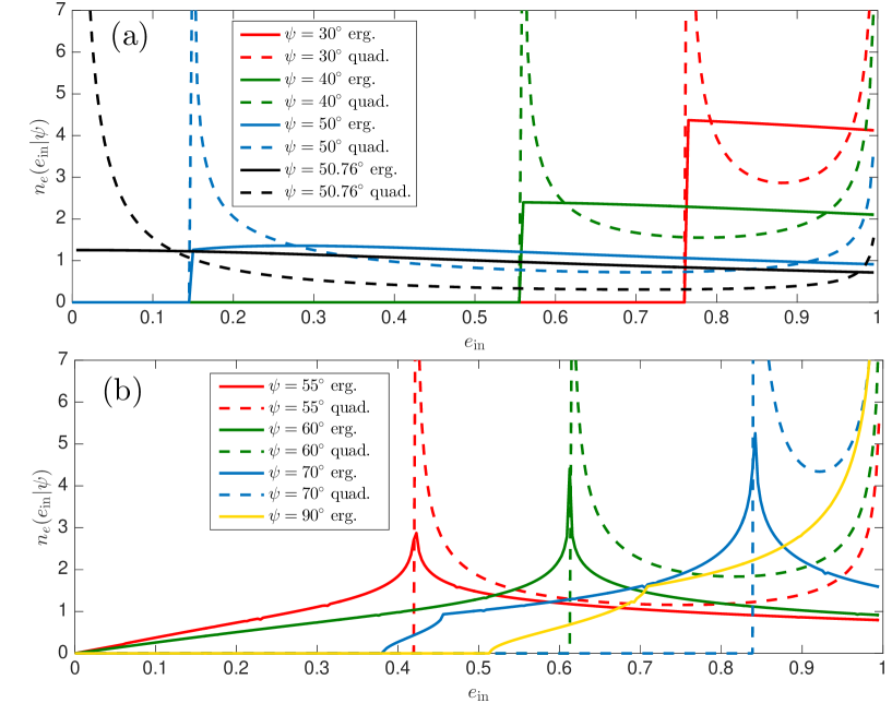
In Figure 1 we show from Equation (A8) for different values of (dashed lines, labeled ‘quad’). We observe that always diverges as and at the minimum eccentricity given by Equation (10). This behavior is expected because the eccentricity oscillations due to the Kozai–Lidov mechanism have turning points at these eccentricities. Also, consistent with our Equation (10), we observe that low eccentricities can only be achieved when ( or )555 In the quadrupole approximation, a test particle reaches a maximum eccentricity at , implying that the minimum inclination is ( and ) if passes through 0 (see the derivation in §5.3.4). From the relation (footnote 4) we observe that trajectories connecting with satisfy so or ..
In summary, in the approximations used here (quadrupole potential and planet of negligible mass) a migrating planet spends most of its time at eccentricities near unity or near a minimum value that depends only on the polar angle of the eccentricity vector at (Eq. 10). The planet reaches low eccentricities during the Kozai–Lidov cycle if and only if this angle is or .
3.3. Ergodic approximation
As described in the previous subsection, in the quadrupole approximation the secular evolution of the inner planet has one degree of freedom and is integrable. This is not generally the case when this approximation is dropped and finding an approximate analytic description of the steady-state eccentricity distribution then becomes more challenging.
In this section, we approach this problem using the ergodic approximation: we assume that the planetary orbits randomly populate all the available phase space allowed by conservation of energy. We shall test this hypothesis using numerical integrations in §3.4. We recall that the derivations in the Appendix used in this section are valid in the test particle regime ().
From Equation (9) we observe that in the quadrupole approximation () the energy of a migrating planet is uniquely determined by —the polar angle of the eccentricity vector at . Therefore, given a value of we can determine a unique time-averaged eccentricity distribution. In the ergodic approximation, the component of angular momentum normal to the perturber orbit, , is uniformly distributed between so we may integrate Equation (LABEL:eq:n_e) over and use Equation (A7) to obtain
| (11) | |||||
where
| (12) | |||||
| (13) |
and is the real part. We note that this integral can be expressed in terms of elliptic integrals, but the expression for arbitrary is somewhat cumbersome and uninformative.
In Figure 1 we show from Equation (11) for different values of (solid lines). We observe that for (top panel) the distribution is relatively flat and restricted to high eccentricity, with a minimum given by Equation (10). This flat profile contrasts with the profile given by the quadrupole approximation, which exhibits strong peaks at and the minimum eccentricity .

For the behavior of changes in nature: the distribution is peaked at an intermediate eccentricity. The position of this peak coincides with the minimum eccentricity in the quadrupole approximation (dashed lines) from Equation (10). The range of eccentricities is significantly wider than in the quadrupole approximation. In particular, small eccentricities can occur for a wide range in . We can estimate this range from Equation (LABEL:eq:n_e) by observing that at low eccentricities the two factors in the square root are only positive for some value of if lies between and 0; and from equation (A7) this requires that is in the range ( in the range ), consistent with Figure 1 (solid lines with ).
From Figure 1 we observe that for all values of , except for the limiting case , the eccentricity distribution predicted by the ergodic approximation is a decreasing function of as it approaches unity. This behavior is different from the quadrupole approximation, in which the eccentricity diverges at . All else being equal, the migration speed is determined by the fraction of time that the planet spends at . Since this fraction is significantly lower in the ergodic approximation (compare solid and dashed lines at ), we expect that the migration speed predicted by the ergodic approximation is much slower than that from the quadrupole approximation.
In summary, the ergodic approximation predicts two families of eccentricity distributions, depending on the polar angle of the eccentricity vector when the planet first starts to migrate (): (i) for the distribution is flat and allows for the same range of eccentricities as that in the quadrupole approximation; (ii) for the distribution is peaked at an intermediate eccentricity and allows for a much wider range of eccentricities than predicted by the quadrupole approximation. Unlike the distribution in the quadrupole approximation, both families of eccentricity distributions are decreasing functions of as it approaches unity, implying slower migration rates.
3.4. Comparison with numerical integrations
We now compare the analytic results for the eccentricity distribution obtained using the ergodic approximation in §3.3 with numerical integrations. These involve solving the secular equations of motion including the gravitational potential of the external perturber up to the octupolar moment (up to ). The equations of motion are given in Petrovich (2015a), after ignoring the non-Keplerian interactions and assuming that all bodies are point masses (no tidal disruptions or collisions).
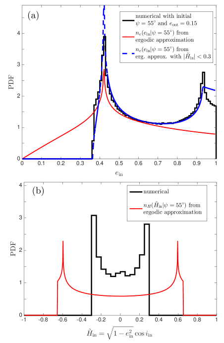
In Figure 2 we show the evolution of (panel a) for one example that starts with an eccentricity vector having magnitude , polar angle , and azimuth 666 For our choice of , the energy in Equation (8) coincides with that in the quadrupole approximation, meaning that the energy in the ergodic approximation (quadrupole-level) and that in the numerical integration (octupole-level) are the same.. We see that the evolution of has a complicated quasi-periodic pattern.
In panel b we show the time-averaged distribution of from the numerical integration (solid black line) and compare this with our analytic distribution with , given by Equation (11) based on the ergodic approximation (solid red line). We observe that the analytic expression describes the position of the peak and the overall shape of the distribution derived from the simulation reasonably well.
In panel c of Figure 2, we show the distribution of to assess whether the ergodic hypothesis is satisfied and the planetary orbit randomly populates all the available phase space. We compare this distribution with that from the ergodic approximation (dashed red line) by integrating Equation (LABEL:eq:n_e) over and using Equation (A7) to obtain
where and are given by Equations (12) and (13). We observe that reproduces the distribution of from the numerical integration reasonably well.
We now repeat the calculations shown in Figure 2, but for a simulation with a lower eccentricity of the perturber, instead of 0.5, which reduces the strength of the octupole relative to the quadrupole (lower in Eq. 7). We show the resulting eccentricity distribution as the black curve in panel a of Figure 3 and observe that this distribution is not reproduced by the ergodic model (red curve, computed using Eq. 11). We also show a blue dashed curve representing the result if the integral in Equation (11) is restricted to the domain ; this ad hoc fix dramatically improves the agreement between the analytic theory and the results from the numerical integrations. We speculate that the lower value of in this example has reduced the strength of the octupole-level perturbations to the point that they can drive the momentum variable to sample only a restricted part of the available region of phase space.
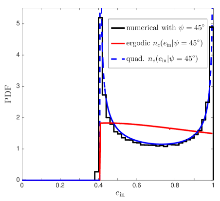
We now repeat the calculation shown in Figure 2 once again, but for a simulation with initial condition instead of . We show the resulting eccentricity distribution in Figure 4 and observe that it is not reproduced by the ergodic model. This disagreement is not surprising because the inner planet in this example evolves only through the range , while the ergodic hypothesis predicts that the orbit should fill the available phase-space ( in from Eq. LABEL:eq:n_e). In fact, we observe that the quadrupole approximation (solid red line), which is equivalent to setting , fits the eccentricity distribution in the simulation much better.
We have tested our analytical results with various other examples and found that when the momentum coordinate reaches values close to the maximum allowed by the conservation of energy (maximum such in Eq. LABEL:eq:n_e), then the ergodic approximation gives a fair description of the eccentricity distribution. If remains small during the integration (say ), then the quadrupole approximation works much better. There are intermediate cases that can be modeled better just by limiting the domain of the integral in Equation (11) to a maximum value of , as we have done in panel a of Figure 3 (dashed blue line).
In summary, the ergodic approximation reproduces the results from numerical simulations reasonably well provided that the specific angular momentum coordinate fills a significant part of its available phase-space. When this is not the case, then either using the quadrupole approximation or restricting the domain of in the ergodic approximation can reproduce the eccentricity distribution from simulations much better.
4. Steady-state eccentricity distribution of warm Jupiters
In this section we calculate the steady-state eccentricity distribution of warm Jupiters, taking into account the time that these planets spend undergoing migration.
The migration speed of a planet is mostly determined by the time it spends at small pericenter distances (high eccentricities). Since tidal dissipation is a very steep function of this pericenter distance, we can approximate the migration speed by a step function as
| (15) | |||||
where and are the critical pericenter distance and eccentricity at which tidal dissipation is efficient enough to cause migration and where is a function of the physical properties of the star and the planet (viscous times, Love number, radii, etc)777The dependence of on arises as follows. At each pericenter passage a planet on a high-eccentricity orbit with a given pericenter distance loses a fixed energy . Thus where is the orbital period. Since we find .. Then, all else being equal and assuming that our choice of allows for significant migration, the steady-state number of migrating planets ( at some point of the eccentricity evolution) as a function of the critical eccentricity is
| (16) |
where the time interval is much longer than the Kozai–Lidov timescale in Equation (1).
Thus, for an ensemble of planetary systems that have time-averaged eccentricity distributions , the expected steady-state eccentricity distribution of the ensemble is
| (17) |
which can be normalized so .
4.1. Numerical experiments
In Figure 5 we evolve 2000 triple systems with parameters , , , , and . The initial conditions are drawn from uniform distributions in the difference in arguments of pericenter and longitudes of node , , and . We evolve the systems for 1000 Kozai–Lidov timescales (Eq. 1) using the secular code described by Petrovich (2015a), after ignoring all the non-Keplerian interactions and treating the bodies as point masses (no tidal disruptions or collisions).
For this simulation we assume that , i.e., planets that achieve maximum eccentricities come close enough to the host star to suffer significant tidal dissipation and therefore migrate. In panel a, we show the initial mutual inclination and planet eccentricity for each system. Planets with are shown as blue or red filled circles. The blue circles indicate the systems with (Eq. 16) larger than the median value (slower migration), while the red circles indicate those with smaller than the median (faster migration).
We see that migrating systems mostly come either from regions where – and or from regions with large eccentricities, . These are excited to high eccentricities through, respectively, the Kozai–Lidov mechanism or low-inclination secular oscillations due to the octupole moment of the perturber. The planets that migrate faster mostly start from either high eccentricities or mutual inclinations .
In panel b of Figure 5, the dashed gray line shows the time-averaged eccentricity distribution of the planets with . We observe that this distribution increases monotonically with , slowly for and faster at higher eccentricities. To obtain the steady-state eccentricity distribution of warm Jupiters we must correct for the migration speed using Equation (17), which yields the solid black line. With this correction, the eccentricity distribution flattens significantly and the peak at high eccentricities is largely eliminated. This result is expected because systems that spend less time at high eccentricities (small pericenter distances) tend to migrate more slowly and thus are more likely to be observed as warm Jupiters at any given time. These results depend only weakly on the choice of the critical eccentricity as long as (or, equivalently ); for example, the distributions are almost identical for (not shown). In other words, the eccentricity distribution from Equation (17) is approximately independent of provided that .
In summary, we find that in these experiments the steady-state eccentricity distribution of migrating planets is broad and approximately flat. Also, this distribution is approximately independent of the semimajor axis provided that migration happens at .
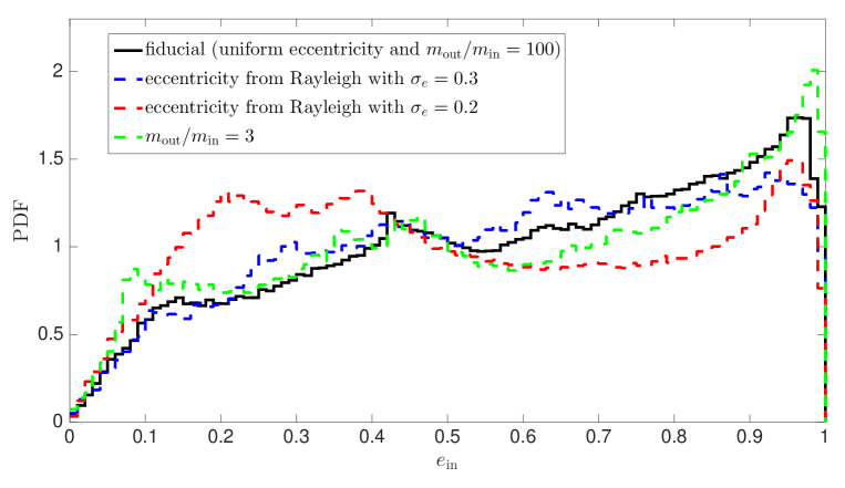
4.1.1 Effect of initial eccentricities and mass ratios
In Figure 6 we repeat the numerical experiments from Figure 5 (shown as the solid black line in the bottom panel), but starting with initial eccentricities of the inner orbit that follow a Rayleigh law,
| (18) |
where is an input parameter that is related to the initial mean and rms eccentricity by and . The red and blue dashed lines show the results for and 0.3, respectively.
We also show the effect of changing the mass ratio of the outer companion from a stellar-mass companion with () to a planetary-mass companion with (green dashed line).
We observe that in all the experiments above the expected steady-state eccentricity distribution for the warm Jupiters from Equation (17) does not change substantially relative to our fiducial simulation. However, the fraction of migrating systems (systems with ) decreases from in our fiducial simulation to and in the simulations with initial eccentricities drawn from a Rayleigh distribution with and , respectively, and to when the mass ratio . This decrease in the number of planets reaching very high eccentricities () for lower mass ratios has been observed by Teyssandier et al. (2013).
We conclude from these numerical experiments that the expected eccentricity distribution of the warm Jupiters predicted by our model is broad and approximately flat, with – of the warm Jupiters having eccentricity less than 0.5.
5. Population synthesis study
We ran a series of numerical experiments to study the evolution of triple systems consisting of a Sun-like host star and two orbiting planets with masses and . We use the full set of equations of motion described in Petrovich (2015a) for hierarchical triple systems; they follow the orbital evolution of the inner and outer planetary orbits and the spins of both the central star and the inner planet including the effects from general relativity, tidal and rotational bulges, and tidal dissipation. These experiments allow us to assess how well our simple model for the steady-state eccentricity distribution in §4—which is based only on the orbit dynamics—works when extra forces are included, and provide explicit predictions for the properties of hot and warm Jupiters formed by high-eccentricity migration.
In our experiments, the inner planet has Jupiter’s mass and radius, and an initial semimajor axis drawn from a uniform distribution in the interval AU, where this narrow range in semimajor axes is chosen for simplicity rather than realism. The outer planet has a mass and semimajor axis that are randomly drawn in the intervals and AU. With this choice of semimajor axes and masses the outer planet can in principle excite large-amplitude eccentricity oscillations in an inner planet with a semimajor axis as small as – AU without this excitation being quenched by general relativity (see Eq. 4).
The initial eccentricity of the inner planet is drawn from a Rayleigh distribution (Eq. 18) with . The eccentricity of the outer planet is drawn uniformly from the interval . The mutual inclination of the inner and outer planets is uniformly distributed in the interval .
We discard systems that do not satisfy the stability condition (Petrovich, 2015c):
| (19) |
where and . The systems that do satisfy this stability criterion are expected to evolve secularly (no exchange of orbital energy between the planets).
The arguments of pericenter and longitudes of the ascending node are chosen randomly for the inner and outer planetary orbits. The host star and the inner planet initially spin with periods of 10 days and 10 hours, respectively. Both spin vectors are parallel to the initial orbital angular momentum of the inner planet (), implying that the initial stellar and planetary obliquities are zero relative to the orbit of the inner planet. We do not include spin-down due to stellar winds in modeling the evolution of the spin of the host star.
We stop each run when one of the following outcomes is achieved: (i) the inner planet evolves into a hot Jupiter in a nearly circular orbit ( AU, ); (2) the inner planet is tidally disrupted, which we define to occur when the pericenter distance is less than 0.0127 AU (Guillochon et al., 2011); (3) the planet has survived for a maximum time chosen uniformly random in the interval . The maximum time is chosen to be 1 Gyr. This is shorter than the typical age of the host stars of warm Jupiters, but our results should be insensitive to so long as it is much larger than the Kozai–Lidov and migration timescales. The typical Kozai–Lidov timescale is yr (Eq. 1). The migration timescale is determined by the planetary viscous time ; we choose this to be 0.01 yr, to allow planets to migrate up to AU with zero eccentricity within 1 Gyr. This is roughly equivalent to setting Gyr and choosing a viscous time of yr (slower migration), but carrying out such simulations would be much more expensive.
We have compared the three-body dynamics predicted by the secular code used in this section to direct N-body integrations using the high-order integrator IAS15 (Rein & Spiegel, 2015), which is part of the REBOUND package (Rein & Liu, 2012). We carried out this comparison for a few representative cases in which the three bodies were treated as point masses, with initial conditions , , , and . We found that the two codes produce similar eccentricity distributions of the inner planet averaged over Kozai–Lidov cycles. The two codes disagree on the relative phases of the eccentricity oscillations of the inner and outer planets, but this disagreement should not affect the general results of our population synthesis study as the planet migration depends mainly on the eccentricity distribution after many oscillation cycles.
5.1. Outcomes
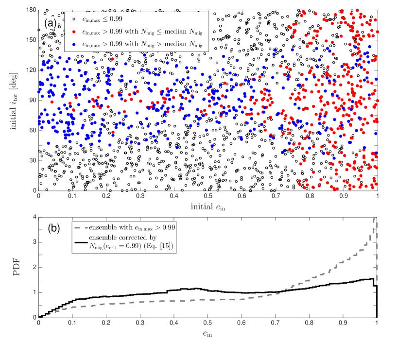
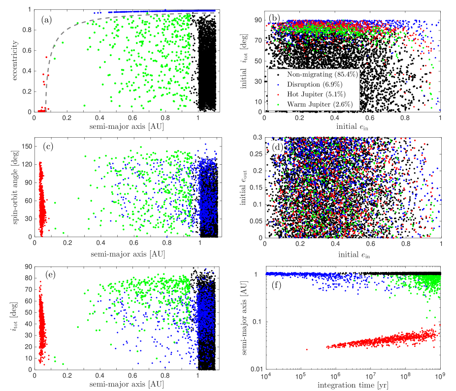
In Figure 7, we show the initial and final orbital elements from our population synthesis study, which followed 15,000 systems that are stable according to Equation (19).
We classify the outcomes as follows (ordered in decreasing frequency):
-
1.
non-migrating (85.4%): The inner planet does not reach eccentricities that are high enough to induce migration. More precisely, these are systems in which the final semimajor axis AU, compared to an initial semimajor axis in the range AU (black dots in Figure 7). Most of these () have mutual inclinations (panel b). The mean eccentricity of the planets in this category increases only from 0.36 to 0.41 from the initial to the final states.
-
2.
disruptions (6.9%): The inner planet is tidally disrupted (blue dots in Figure 7). Disruption is defined to occur when AU at some point of the simulation (Guillochon et al., 2011). Most disruptions () happen very early in the simulation, within Myr of the start (panel f), and most of these systems start with high mutual inclinations (median , panel b).
-
3.
hot Jupiters (5.1%): The inner planet becomes a hot Jupiter (red dots), with AU. The hot Jupiters are formed at a wide range of times between 1 Myr and 1 Gyr (panel f); the median formation time is Myr. Most of these systems start with high mutual inclinations (median , panel b).
-
4.
warm Jupiters (2.6%): The inner planet has semimajor axis in the range from 0.1 AU to 0.95 AU at the end of the simulation (green dots). The warm Jupiters have a median integration time of Myr (panel f) because they are followed for a time chosen uniformly random between 0 and 1 Gyr (see discussion at the end of the preceding subsection). Most of these systems start with high mutual inclinations (median , panel b).
In our model all warm Jupiters would eventually evolve into hot Jupiters given enough time. Therefore, the relative abundance between hot and warm Jupiters is age-dependent and we expect to observe more hot Jupiters per warm Jupiter in older systems.
In summary, our population synthesis model predicts that in most triple systems with parameters similar to those we have chosen the inner planet does not migrate significantly and its eccentricity increases only slightly relative to its initial value. The systems that migrate to form either hot Jupiters or warm Jupiters generally start from high mutual inclinations. The ratio of hot Jupiters to warm Jupiters increases with the age of the system.
5.2. Production rate of hot and warm Jupiters
In the study presented in the previous subsection, the fractions of systems that form hot and warm Jupiters are and , respectively. These fractions depend on the initial conditions, most critically on the distribution of mutual inclinations (see panel b in Figure 7). Since we only have weak observational constraints on the relevant properties of hierarchical planetary systems, we cannot provide meaningful estimates of the production rates of warm and hot Jupiters by this process. However, the ratio of hot to warm Jupiters seen in the simulations, , is not strongly dependent on the initial conditions. In particular, changing the Rayleigh distribution describing the initial eccentricity distribution from to results in a similar ratio, ; changing to a uniform initial eccentricity distribution in the range changes the ratio only to . Similarly, changing the initial distribution of mutual inclinations from a uniform distribution in to a Rayleigh distribution with () changed the ratio of hot to warm Jupiters only to .
We can compare this ratio to the ratio of the number of systems with hot and warm Jupiters in the RV sample, . Thus, the population synthesis studies indicate that our mechanism is more efficient at forming hot Jupiters relative to warm Jupiters than what is observed in the RV sample by a factor –.
As discussed in §5.1, the ratio of hot to warm Jupiters is expected to increase with the age of the system. Although we ran our simulations only for 1 Gyr, we argued in §5 that the results from our simulations should be unchanged if we increase the maximum integration time and the migration timescales (defined by the planet’s viscous time ) by the same factor. Thus we believe that the ratio of hot to warm Jupiters given by our simulations is realistic. Note that the integration and migration timescales should also be constrained to reproduce (if possible) the semimajor axis distribution of the hot Jupiters (see §5.3.2).
In conclusion, even though the production rates of hot and warm Jupiters depend strongly on the initial conditions, their relative rates do not. We find that the ratio between the number of systems with hot Jupiters and the number of systems with warm Jupiters is roughly 2. This ratio is larger than that in the observations by a factor of –5, so we expect that our mechanism can only form up to – of the warm Jupiters even if it produces all of the hot Jupiters.
5.3. Orbital distributions of hot and warm Jupiters
In this section we describe the distributions of orbital elements arising from our population synthesis study (see Figure 7). We compare the results from our model with the observed semimajor axis and obliquity distributions in §5.3.2 and §5.3.3 respectively, while reserving the comparison with the eccentricity distribution for a separate and more in-depth section in §6.
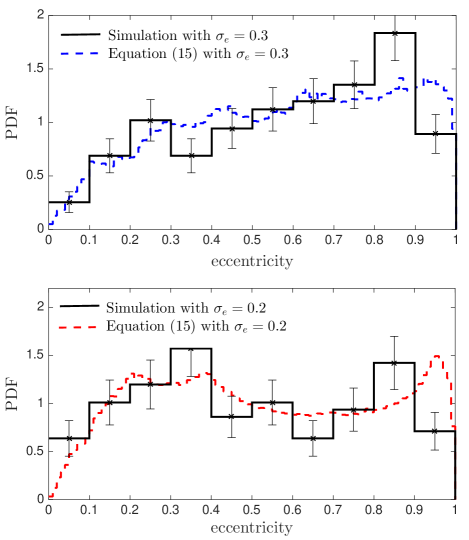
5.3.1 Eccentricities
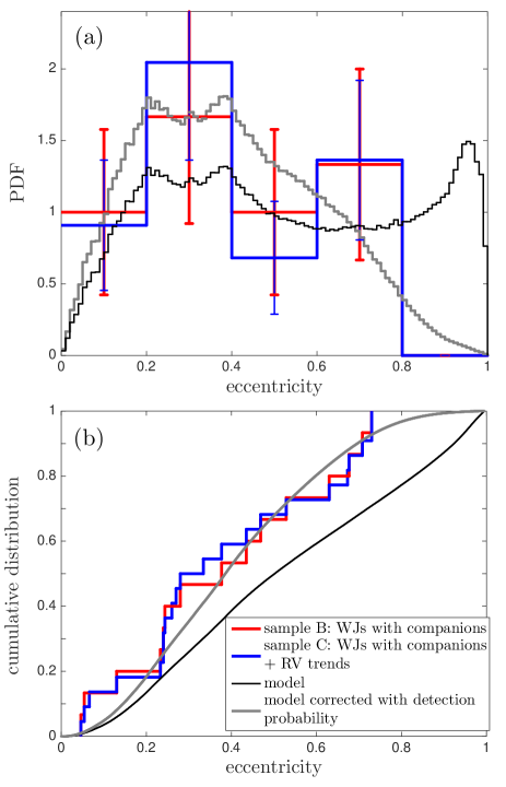
In the upper panel of Figure 8 we show the eccentricity distribution of the warm Jupiters from the simulation shown in Figure 7, in which the initial eccentricities are chosen from a Rayleigh distribution with . The lower panel is similar, but the initial eccentricities are chosen from a distribution with . We compare our results with the steady-state eccentricity distribution from Equation (17) with critical eccentricity and a fixed perturber (, AU, and ), shown as dashed blue and red lines.
We observe that the simple model in §4 broadly reproduces the distribution from the simulations. However, there are small but significant differences at very high eccentricities: the simulation has fewer planets at than the model predicts, and more in the region . These differences probably arise because the warm Jupiters in our simulations are constrained to a maximum eccentricity given by AU (dashed line in panel a of Figure 8)—planets having less angular momentum than this track are either tidally disrupted or form hot Jupiters. In contrast, our simple model ignores tidal disruption and circularization, allowing for warm Jupiters with arbitrarily large eccentricities and thereby overpopulating the bin relative to our simulations.
In summary, our simple model for the steady-state eccentricity distribution in §4 reproduces well the results from our population synthesis study, even though it ignores the effects from general relativity, tides, and disruptions. The simple model predicts a somewhat larger number of warm Jupiters with the highest eccentricities because it does not account for tidal disruption and tidal dissipation.
5.3.2 Semimajor axes
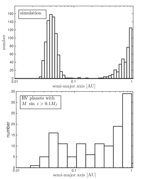
In the upper panel of Figure 9 we show the semimajor axis distribution of the migrating planets (hot and warm Jupiters) from the population synthesis study shown in Figure 7. The lower panel shows the semimajor axis distribution of planets with AU discovered in radial-velocity (RV) surveys.
Our simulations predict that the number density of warm Jupiters per unit of increases with , with of the warm Jupiters between 0.1 and 1 AU having semimajor axes larger than 0.4 AU. In contrast, the observed sample has of the planets in the semimajor axis range inside 0.4 AU.
Our model also produces a population of hot Jupiters at AU with a pile-up at – AU. Quantitatively, the distribution of semimajor axes of the hot Jupiters in the simulation matches that of the observed hot Jupiters with AU in the RV sample (-value of from a Kolmogorov–Smirnov [KS] test). The observed population of hot Jupiters at AU, which are not present in our simulation, could be produced by enhancing the tidal dissipation in the planet.
In summary, our population synthesis study fails to reproduce the observed semimajor axis distribution of warm Jupiters in the range – AU. The simulation does reproduce the shape of the semimajor axis distribution in the ranges 0.5–1 AU and inside 0.07 AU.
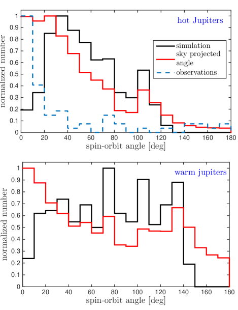
5.3.3 Stellar obliquities
In Figure 10 we show the final spin-orbit angle (or stellar obliquity, angle between the host star’s spin axis and planet’s orbital axis ) of the hot and warm Jupiters in our simulations (upper and lower panels, respectively). We also calculate the distribution of sky-projected spin-orbit angles (red lines) by randomizing the orbital configurations relative to a fixed observer. The sky-projected angles can be directly compared to the observed angles as determined by the Rossiter-McLaughin effect (e.g., Fabrycky & Winn 2009; Crida & Batygin 2014). For comparison we show the sample of 65 hot Jupiters with stellar obliquity measurements in the upper panel (blue dashed line). We do not plot the observations of warm Jupiters because the sample size is too small for a meaningful comparison.
We observe that the obliquities of the hot Jupiters in the simulation are concentrated in the interval –. The simulations produce retrograde hot Jupiters, similar to the fraction in the observed sample of . The projected obliquity distribution of the simulated hot Jupiters (red line in the upper panel) peaks at small values, similar to the observed distribution. However, the observed sample has a strong peak at low obliquities— of the hot Jupiters have projected obliquities of —compared to only in our simulations. Apart from this discrepancy at low obliquities, the observed and model distributions match reasonably well.
In the lower panel of Figure 10 we show the obliquity distribution of the warm Jupiters, which is significantly broader than that of the hot Jupiters. In particular, of the warm Jupiters have retrograde obliquities compared to of the hot Jupiters. There are only 2 warm Jupiters with measured obliquities, too few to plot on the lower panel of Figure 10.
We note that the KL timescales in our simulated systems are small ( yr from Eq. [1]) compared to the spin precession timescale due to the rotation-induced stellar quadrupole ( yr). Therefore, the stellar obliquity distribution is unaffected by the secular resonance that occurs when the stellar precession rate matches the orbital precession rate as described in Storch at al. (2014) and Storch & Lai (2015).
5.3.4 Mutual inclinations
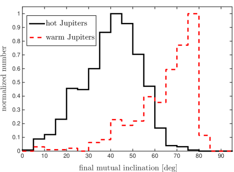
In Figure 11 we show the distribution of the mutual inclinations between the inner and outer planetary orbits for the systems with hot Jupiters (solid black line) and warm Jupiters (dashed red line).
Systems with hot Jupiters tend to have mutual inclinations clustered around . This peak in the inclination distribution is a known feature of Kozai–Lidov migration in the quadrupole approximation (Fabrycky & Tremaine, 2007), which can be explained as follows. Let us treat the planet as a test particle for simplicity888The argument does not depend critically on this approximation (see Fabrycky & Tremaine 2007).. The conservation of angular momentum normal to the outer orbit and the energy in Equation (A2) implies that the following is a conserved quantity:
| (20) |
A planet can migrate to form a hot Jupiter when it reaches a sufficiently large maximum eccentricity . At this point the inclination is a minimum (or a maximum if the orbit is retrograde) because of the conservation of . The maximum eccentricity in a Kozai–Lidov cycle is achieved at . Thus,
| (21) |
If the orbit passes through at any point in the cycle, Equation (20) implies that and from Equation (21) we have ( and ). Therefore, if we start from nearly circular orbits, we expect that the hot Jupiters should have a distribution of mutual inclinations that peaks strongly at for prograde orbits.
The dispersion around in our simulations is . This dispersion has several distinct causes: (i) the initial eccentricity of the inner planet is not precisely zero, as it follows a Rayleigh distribution with ; (ii) the octupole-level forcing from the outer companion allows for migration from orbits with mutual inclination lower than (Petrovich, 2015b); (iii) the quantity is not precisely conserved when the octupole-level perturbations from the outer companion are included (Naoz & Fabrycky, 2014).
The peak of the distribution of mutual inclinations is relatively insensitive to the initial eccentricity distribution: it changes from for an initial eccentricity distribution drawn from a Rayleigh distribution with to and for a Rayleigh distribution with and uniform in , respectively. Also, we note that our initial conditions are constrained to and if we relax this assumption allowing for we would expect an extra peak at (Fabrycky & Tremaine, 2007).
The warm Jupiters generally have much larger mutual inclinations than the hot Jupiters (Fig. 11). This difference arises mainly because the mutual inclination of the warm Jupiters reflects the time-averaged distribution of the ensemble, not the minimum values as it is case for the hot Jupiters.
In summary, the systems with hot Jupiters in our population synthesis study tend to have outer planetary companions with mutual inclinations clustered at around , while most of the systems with warm Jupiters have companions with mutual inclinations .

6. Eccentricity distribution of the observed warm Jupiters
We compare the eccentricity distribution in our simulations to three samples of exoplanets999We take the data from http://exoplanets.org (Wright et al., 2011) and http://exoplanet.hanno-rein.de/ (Rein, 2012) as of September 2015.:
- A
-
All exoplanets discovered in radial-velocity surveys with masses and semimajor axes –1 AU (these limits correspond to the definition of warm Jupiters used throughout this paper). This sample consists of 102 planets in 96 planetary systems, and has a mean eccentricity of 0.26. In Figure 12 we show the density (panel a) and cumulative distribution (panel c) of the eccentricities in this sample (solid black lines). The density distribution peaks at and decays monotonically for higher eccentricities. In contrast, our model predicts a flat eccentricity distribution (no peak at ) and thus does not match the observed distribution in this sample.
- B
-
The planets in sample A that have relatively well-separated outer companion planets ( AU and 101010This choice is somewhat arbitrary. It excludes two systems with planets in 2 : 1 mean-motion resonances, HD 82943 (Tan et al., 2013) and HD 73526 (Tinney et al., 2006), whose orbital configuration are likely due to disk migration.. The motivation for this choice is that our model predicts that the warm Jupiters should have planetary companions in orbits outside AU. This sample consists of 15 planets; the mean eccentricity of 0.38 is significantly larger than in sample A. We show the eccentricity distribution of this sample in Figure 12 using solid red lines. The distribution is flatter than sample A; a KS test between the distribution in the samples AB (dashed green lines) and B results in a p-value of 0.08. Sample B is consistent with a uniform distribution in the eccentricity range (dotted black lines in Figure 12).
- C
-
Sample B augmented by systems from sample A that exhibit linear trends in radial velocity, which indicate the presence of a long-period planet or a stellar companion. These companions are likely to be far enough so the eccentricity oscillations of the warm Jupiters with the smallest semimajor axes are quenched by relativistic precession (see discussion in §2). Thus, we only add a system with a radial-velocity trend if the semimajor axis of the warm Jupiter is AU (see Eq. 4). This sample totals 22 planetary systems and is shown by solid blue lines in Figure 12. This distribution is similar to the distribution of sample B and significantly flatter than of sample A; a KS test between the distribution in the samples AC (dashed grey lines) and C results in a p-value of 0.02.
The finding that warm Jupiters with outer planetary companions have a flatter eccentricity distribution than the whole sample of warm Jupiters is originally due to Dong et al. (2014). We confirm their results, but for a bigger sample: 9 planets in Dong et al. (2014) compared to 15 planets (or 22 considering the RV trends) in our study. The difference in the sample size is due to the larger ranges of masses we consider ( compared to in Dong et al. 2014) and the larger range of semimajor axes ( AU in our work compared to AU in Dong et al. 2014).
In summary, we observe that the eccentricity distribution of the sample of warm Jupiters is skewed towards low eccentricities, but the subsample of systems with outer planets (either RV detections or RV linear trends) is approximately flat for eccentricities in the range .
6.1. Comparison with our model
In §4 we showed that the steady-state eccentricity distribution predicted by our model is relatively flat in and largely independent of the initial distribution of eccentricities of the inner planet (see Figure 6).
In Figure 13, we compare the eccentricity distribution predicted by our model in which the initial eccentricities are drawn from a Rayleigh distribution with (solid black lines) to samples B and C. We observe that the model reproduces, at least qualitatively, the overall flat profile of the observed eccentricity distribution up to . However, the model fails to account for the lack of planets with in the observations.
One possible reason for the absence of highly eccentric () planets in the observations is the selection effects in RV surveys against detecting planets with —sparse observations of high-eccentricity orbits are likely to miss the strong reflex velocity signal near pericenter, leading to non-detection of planets that would be detected at the same semimajor axis and smaller eccentricity (Cumming, 2004; O’Toole et al., 2009). This possibility is discussed further in the following subsection.
6.1.1 Correcting for eccentricity selection bias
We briefly discuss how observational selection biases against detecting high-eccentricity planets (Cumming, 2004) could bring our results into closer agreement with the observations. We emphasize that this discussion is for illustration only and is not a quantitative analysis of the effects of selection bias.
Motivated by the results in Cumming (2004, Figure 4) we parametrize the eccentricity dependence of the detection probability in radial-velocity surveys as
| (22) |
where represents the detection threshold for a given signal-to-noise ratio and number of measurements (for the signal is detected half of the time). The quantity represents the characteristic width of the detection probability around .
In Figure 13 we show the results of the model eccentricity distribution corrected by Equation (22) with and (solid gray lines). Although this choice of parameters is somewhat arbitrary, it is motivated by one of the models of Cumming (2004), who shows that the detection probability with signal-to-noise ratio 10 and observations is 1 for and drops to 0.5 and 0.1 for and , respectively.
Our corrected eccentricity distribution fits the observed distribution very well. The -values from a KS test comparing our model distribution with samples B and C increase from and when no correction is applied to 0.88 and 0.44 when we correct the distribution.
These results are largely independent of the initial eccentricity distribution in the simulations and similar results are obtained for a uniform distribution and a Rayleigh distribution with . Our simulated eccentricity distributions can match the data on warm Jupiters with outer companions for various functional forms of the detection probability provided that it drops from at to small values (say ) at .
In summary, our model can match the observed eccentricity distribution of the warm Jupiters with outer companions when plausible selection biases against detecting highly eccentric planets are taken into account.
7. Discussion
We have examined the expected eccentricity distribution of warm Jupiters that migrate through a combination of secular gravitational interactions with a distant companion and tidal dissipation (“high-eccentricity migration”). Our main result is that the expected distribution is approximately flat (). This result partially resolves the well-known problem that warm Jupiters cannot have reached their current semimajor axes through high-eccentricity migration because their pericenter distances are too large to allow for significant tidal dissipation by the host star.
However, our model cannot fully reproduce the eccentricity distribution of the warm Jupiters because it does not produce enough planets with eccentricities (Figure 12). This discrepancy is eliminated if we consider only warm Jupiters in systems containing outer planetary companions or linear RV trends suggesting a distant stellar or planetary companion—and of course such a companion is required in our model.
The population of low-eccentricity warm Jupiters () must be largely formed by a different mechanism. Most likely, these planets acquired their current orbital configurations when the gaseous disk was still present, either by disk migration (Goldreich & Tremaine, 1980; Ward, 1997) or in-situ formation (e.g., Batygin et al. 2015; Boley et al. 2015; Huang et al. 2016).
In what follows, we describe other results and predictions from high-eccentricity migration and compare our work with previous studies.
7.1. Contribution from our model to the hot Jupiter population
We discuss how the hot Jupiter population produced in our simulations of high-eccentricity migration compares to the observed population.
First, in our simulations the ratio between the number of hot Jupiters and the number of gas giant planets is –. This ratio is consistent with the observed rate of –, derived using the occurrence rate of hot Jupiters, – (Gould et al., 2006; Mayor et al., 2011), and that of gas-giant planets at AU distances, (Mayor et al., 2011). However, the hot Jupiter production rate derived from our models depends strongly on the initial conditions because the planets migrate only if they initially have either high mutual inclinations or large eccentricities (panel b in Figure 7).
Second, as discussed in §5.3.2 and shown in Figure 9, our model predicts that the semimajor axes of hot Jupiters are strongly concentrated in the range – AU (orbital period of – days), roughly consistent with the distribution observed in both the RV and Kepler samples (Santerne et al., 2015). This pile-up arises because there is a minimum pericenter distance at which the eccentricity excitation is limited by extra precession forces (general relativity and/or tidal bulges, see Wu & Lithwick 2011 and Petrovich 2015b).
Third, the obliquity distribution predicted by our population synthesis model is broad (see upper panel in Figure 10). We successfully reproduce the observed ratio between the numbers of retrograde and prograde systems, but fail to explain the sharp peak in the distribution at projected obliquities produced by of the observed sample of hot Jupiters. Roughly of the hot Jupiters with low obliquities ( of the current sample), must be produced by a different mechanism.
In summary, based on the production rates, the semimajor axis and stellar obliquity distributions we suggest that high-eccentricity migration can account for most of the hot Jupiters. A fraction of the low-obliquity hot Jupiters must be formed by a different mechanism.
7.2. Contribution from our model to the warm Jupiter population
We discuss how the warm Jupiter population produced in our simulations compares to the observed population.
Our model can explain the eccentricity distribution of warm Jupiters observed in samples B or C of §6, i.e., the 15 systems with outer planetary companions or the 22 systems with companions or RV trends. For comparison the total number of systems with warm Jupiters is 96. Thus, our model can potentially account for to of the whole population of warm Jupiters—more in the likely case that not all companions have been detected so far.
An independent estimate of the production rate of warm Jupiters is given by our population synthesis models. As discussed in §5.2, we find that the relative rates of production of hot and warm Jupiters do not depend strongly on the initial conditions, and our model predicts that the ratio of hot Jupiters to warm Jupiters should be roughly 2. This is larger than the observed ratio in the RV sample, , by a factor of –. Therefore, if our mechanism accounts for most of the hot Jupiters (see previous subsection), then we expect that it also accounts for – of the systems with warm Jupiters, consistent with the estimate from the preceding paragraph.
In summary, by comparing the relative production rates of hot and warm Jupiters with the inferred values from observations, we conclude that our mechanism can account for – of the systems with warm Jupiters. This number matches the fraction of derived from the eccentricity distribution of warm Jupiters in systems with outer companions.
7.3. Predictions
We have shown that our model can account for most of the hot Jupiters and of the warm Jupiters.
Two natural predictions from the high-eccentricity migration model discussed in this paper are: (i) the presence of long-period planetary companions in most of the hot Jupiter systems; (ii) the presence of long-period planetary companions in at least of the warm Jupiter systems, typically those in which the warm Jupiter has .
Recent studies show that the occurrence rate of distant (– AU) planetary-mass companions of hot Jupiters is , which is consistent with the prediction that high-eccentricity migration can account for most of the hot Jupiters (Knutson et al., 2014; Bryan et al., 2016). Similarly, Bryan et al. (2016) constrain the occurrence rate of long-period ( AU) planetary-mass companions of warm Jupiters to . This number is larger than the predicted by our model of high-eccentricity migration, but we expect that a fraction of these systems with the most distant of the planetary companions do not contribute to the warm Jupiter formation because the KL oscillations can be quenched by GR (see Eq. 4).
In what follows, we discuss additional observational tests that can further constrain our model using upcoming observational capabilities.
7.3.1 Mutual inclination angles of hot and warm Jupiters systems with outer companions
As discussed in §5.3.4 our model predicts that the systems with hot and warm Jupiters should have outer planetary companions in inclined orbits.
For hot Jupiters, we find that the distribution of mutual inclinations peaks at with a spread of around this value (see the black line in Figure 11). As discussed in §5.3.4, this peak is a feature of the Kozai–Lidov oscillations of the inner planet in which the planet circularizes when it reaches a maximum eccentricity, which generally happens at a minimum inclination close to .
In contrast, the warm Jupiters should have companions with larger mutual inclinations than the hot Jupiters, typically in the range – (see Figure 11). As described in §5.3.4, the larger value arises because hot Jupiters are found at the minimum inclination achieved during a Kozai–Lidov cycle, while the warm Jupiters represent the steady-state inclination distribution during a cycle.
At present little is known about the mutual inclinations of massive planets. A notable exception is an astrometric measurement of the mutual inclination of And c and d, (McArthur et al., 2010). We expect that the GAIA space telescope can measure this angle for many of the hot and warm Jupiters with detected outer companions out to AU (e.g., Casertano et al. 2008; Sozzetti et al. 2014).
7.3.2 Spin-orbit angles of warm Jupiters
As discussed in §5.3.3 we expect that the warm Jupiters formed by secular planet-planet interactions will have an approximately uniform distribution of stellar spin-orbit angles in the range – (see the lower panel in Figure 10). Future space missions such as TESS (Ricker et al., 2014) and PLATO (Rauer et al., 2014) will discover hundreds or even thousands of warm Jupiters in bright stars amenable to Rossiter-McLaughin measurements of the projected spin-orbit angle. Ground-based transit surveys are also expected to find many warm Jupiters, with periods days (see, e.g., Bakos et al. 2013 for a discussion on the expected rates). Two recent examples are HATS-17b with a period of 16.3 days Brahm et al. (2016) and WASP-130b with a period of 11.2 days Hellier et al. 2016.
It would be particularly informative to compare the obliquities of the warm Jupiters in eccentric orbits with outer companions, which can likely be explained by high-eccentricity migration, to a sample of low-eccentricity warm Jupiters without outer companions, which must have formed by a different mechanism and presumably have much smaller obliquities.
7.4. Comparison with other work
We discuss our results in the context of recent work on high-eccentricity planet migration.
Dawson & Chiang (2014) suggested that a population of 6 systems with eccentric warm Jupiters and outer planetary companions might be undergoing Kozai–Lidov migration. This claim is based on the clustering of the relative apsidal angles of these planets at around . Since the outer companions in these systems are eccentric (–) and the Kozai–Lidov oscillations are modulated by the octupole timescale, the authors argue that these planets are undergoing a slow version of Kozai–Lidov migration, which preferentially produces warm Jupiters over hot Jupiters.
Our results are consistent with Dawson & Chiang (2014) in the sense that we find that in a steady state the planets that are most likely to be observed as warm Jupiters tend to have a significant octupolar modulation of the eccentricity oscillations (because such planets spend less time at very high eccentricities and therefore have slower migration rates). In particular, in Figure 1 we show the family of eccentricity distributions for a migrating planet in two limits: the quadrupole approximation (no octupole contribution) and the ergodic approximation (strong octupole contribution). This figure shows that in the quadrupole approximation the eccentricity distribution diverges as , while in the ergodic approximation the distribution is a decreasing function of the eccentricity as . However, contrary to the results by Dawson & Chiang (2014), we do not observe a significant clustering of the relative apsidal angles (, the difference in the longitudes of pericenter measured relative to the invariable plane) around in our simulated systems containing warm Jupiters. These results suggest that either (i) the clustering observed by Dawson & Chiang, which looks persuasive but is based on only six systems containing a warm Jupiter and an outer companion, is an unlikely statistical fluke; (ii) the clustering arises through some unrecognized selection effect; or (iii) the clustering arises for particular ranges of other other orbital elements that are much more densely populated in real systems containing warm Jupiters than in our simulations. These issues deserve further investigation.
Petrovich (2015b) proposed that most hot Jupiters, but almost no warm Jupiters, could be formed by a process he called “coplanar high-eccentricity migration”—secular interactions of two nearly coplanar eccentric planets. Consistent with these results we find that planets starting with low mutual inclinations and high eccentricities migrate rapidly (see panel a of Figure 5) and are, therefore, expected to produce hot Jupiters rather than warm Jupiters.
Frewen & Hansen (2015) have recently studied the possibility that a population of warm Jupiters migrating through the KL mechanism can be depleted as the host star evolves off the main sequence and grows in radius. These authors study the eccentricity distribution of the warm Jupiters and, in contrast to the present paper (see Figure 8), find that the eccentricity distribution is strongly peaked at low eccentricities (Figure 17 of Frewen & Hansen). We may understand this difference from the particular set of initial conditions used by Frewen & Hansen (2015), in which the inner and outer planet both start on nearly circular orbits (). This choice limits the family of eccentricity distributions in Figure 1 to only one, which would be approximated by the dashed black and blue lines in the top panel of Figure 1 (quadrupole approximation with ). However, their calculations do not show the extra lower-amplitude peak at found in our quadrupole distributions, possibly because this peak is shifted to a range of lower values in since their warm Jupiters are initialized at AU and reach minimum pericenter distances AU. Note that even if the inner planet starts in a circular orbit, but the perturber is eccentric so its potential has a significant octupolar moment, the expected eccentricity distributions are generally not peaked at low eccentricities (see solid lines in Figure 1).
Very recently, Antonini et al. (2016) carried out a numerical study of the formation of hot and warm Jupiters from Kozai–Lidov oscillations induced by planetary perturbers. Consistent with our main result, their simulations show that the warm Jupiters formed by this mechanism have a nearly flat eccentricity distribution. However, the authors claim that most of the observed warm Jupiters with outer planetary companions are not formed through high-eccentricity migration. Their claim is based on the observation that if the inner planet in these systems started migration beyond AU, then these systems would have been dynamically unstable. While the dynamical stability of the pre-migration system is an important constraint on the observed systems, all of the systems in our population synthesis study are stable (according to Equation 19) so this result does not affect our numerical experiments.
7.5. Stellar binary vs. planetary-mass outer companion
The main results of this paper are valid whether the outer perturber is a planet or a star (see, e.g., Figure 6). We have assumed a planetary-mass companion in most of our discussion, motivated by the observation that warm Jupiters in systems with outer planets have a broad eccentricity distribution consistent with our model, whereas those in systems without outer planets mostly have . Here we briefly discuss what conditions are required for the stellar-companion scenario to explain the warm Jupiters.
As discussed in §2, there are at least two conditions for a migrating warm Jupiter to be undergoing eccentricity oscillations:
-
•
The migration rate must be slow relative to the secular perturbations. As shown by Petrovich (2015a), the Kozai–Lidov mechanism in wide stellar binaries ( AU) generally leads to fast migration and, therefore, produces almost no warm Jupiters (similar results are shown in Anderson et al. 2016). This behavior is mostly due to the strong octupole-level modulation of the Kozai–Lidov mechanism in stellar binaries, which pumps up the eccentricity to extremely high values, enhancing the fraction of the planets that migrate rapidly (in the sense of Equation LABEL:eq:r_p) or are tidally disrupted. We expect that this effect is more pronounced in stellar binaries for two different reasons. First, stellar binaries are more eccentric (mean eccentricity of at separations of AU; e.g, Tokovinin & Kiyaeva 2015) than the cold Jupiters (mean eccentricity of ) and, therefore, the octupole forcing can have more dramatic effects in stellar binaries (e.g., Lithwick & Naoz 2011; Katz, Dong, & Malhotra 2011). Second, contrary to the case of stellar companions, the orbits of planetary companions can change their angular momentum significantly in timescales comparable to that of the octupole, often leading to less extreme eccentricities (e.g., Teyssandier et al. 2013).
-
•
Precession due to secular perturbations has to be faster than the precession due to general relativity. From Equation (4) we observe that this requirement implies that warm Jupiters within AU must have stellar binary companions with masses of () within AU ( AU). The frequency of stellar companions at these orbital separations in warm-Jupiter systems remains largely unconstrained, and the constraints on stellar companions in hot-Jupiter systems are difficult to interpret. Recently Piskorz et al. (2015) searched for low-mass stellar companions within AU around systems with hot Jupiters (not warm Jupiters). They found no evidence of an excess of binary companions relative to field stars, suggesting that hot Jupiters are not preferentially formed in these systems. Then, if most hot Jupiters are not formed by the KL mechanism in stellar binaries within AU, we expect that only a small fraction of the warm Jupiters can be explained by this channel because our numerical experiments indicate that the rate of formation of hot Jupiters is higher that of warm Jupiters (a factor of for binaries, see below), while the observations indicate the opposite—there are twice as many warm Jupiters than hot Jupiters. On the other hand, Wang et al. (2015) recently found evidence that the stellar multiplicity fraction of companions at AU is a factor of higher for stars hosting a gas giant planet candidate from the Kepler sample, compared to a control sample with no planet detections.
We have carried out a population synthesis study similar to that in Figure 7, but changing the semimajor axis and mass ranges of the perturber from – AU and to – AU and , so the the amplitude of the quadrupole potential in Equation (6) lies roughly in the same range. We observe that the ratio of hot Jupiters to warm Jupiters formed in these simulations is , compared to in the planetary case. We also repeated the experiment with a broader eccentricity distribution—uniform in over compared to , which is more appropriate for stellar binaries111111We discard the systems that do not satisfy the stability criterion of Mardling & Aarseth (2001).. As expected from our previous discussion, we find that the ratio of hot Jupiters to warm Jupiters increases, from to . Finally, we checked that the eccentricity distributions of the warm Jupiters from these experiments are consistent with those from our simple models in §4.
In conclusion, the eccentricity distribution of the warm Jupiters predicted by our model is approximately flat regardless of the whether the outer perturber is a planet or a star. However, the ratio of warm Jupiters to hot Jupiter is lower (by a factor ) in the binary-companion case compared to the planetary-companion case, making the latter channel a more likely explanation of the warm Jupiters.
7.6. The ergodic approximation
In §3.3 we have explored a new analytical model to approximate the time-averaged eccentricity distribution of the inner binary in a hierarchical triple system. This model is based on the ergodic hypothesis, in which we assume that the planetary orbits randomly populate all the available phase space allowed by conservation of energy.
We have shown that this model can reproduce the eccentricity and momentum coordinate distributions obtained from numerical three-body integrations when the inner orbit populates a significant fraction of its available phase-space (see Figure 2). This last condition is satisfied when there is a strong octupole-level gravitational perturbation from the outer orbit. For simplicity our discussion assumed that the inner body is a test particle, but the model can be extended to massive inner bodies.
The ergodic hypothesis is motivated by the observation that a distribution function that is uniform on the energy surface in a canonical phase space is always a solution of the collisionless Boltzmann equation if the motion is governed by a Hamiltonian (e.g., Binney & Tremaine, 2008). Thus we expect the distribution of systems over the energy surface to be uniform if either the initial conditions sample the phase space uniformly or the motion is sufficiently irregular that the trajectory samples most of the phase space.
A more speculative application of the ergodic hypothesis to planetary systems is described by Tremaine (2015).
8. Conclusions
We have studied the steady-state orbital distribution of giant planets migrating through the combination of secular gravitational perturbations due to a planetary or stellar companion and friction due to tides raised on the planet by the host star (“high-eccentricity migration”).
We have shown both analytically and numerically that the eccentricity distribution of warm Jupiters arising from this migration mechanism is approximately flat. This distribution is inconsistent with the observed eccentricity distribution of all of the warm Jupiters, which decays approximately linearly from to (Fig. 12), but roughly consistent with the eccentricity distribution of warm Jupiters with detected outer planetary companions, such as would be required for high-eccentricity migration to occur.
Both the observed eccentricity distribution and the observed ratio of hot Jupiters to warm Jupiters are consistent with a model in which of warm Jupiters and most of the warm Jupiters with eccentricity are produced by high-eccentricity migration.
We also find that high-eccentricity migration induced by a distant planetary companion can account for the semimajor axes, the stellar obliquities, and occurrence rates of most of the hot Jupiters.
Thus we are led to a model in which (i) high-eccentricity migration produces most of the hot Jupiters; (ii) high-eccentricity migration produces the of warm Jupiters with ; (iii) most of the remaining population of low-eccentricity warm Jupiters must be accounted for by a different mechanism.
We also provide predictions for the mutual inclinations, spin-orbit angles, and other properties of the hot and warm Jupiters produced by high-eccentricity migration that can be used to test this model.
Appendix A Time-averaged eccentricity distribution in a quadrupole potential
We calculate the time-averaged eccentricity distribution for the orbit of an inner test particle that evolves due to the quadrupole potential from an external body. We work in a coordinate system centered on the host star, of mass , in which the equator coincides with the orbit of the outer body. We use Delaunay elements , , ; their conjugate angles , , are respectively the mean anomaly, argument of pericenter, and longitude of the node of the test particle.
The doubly time-averaged Hamiltonian that represents the gravitational potential of the outer body up to quadrupole order is obtained by converting equation (3.1) to orbital elements and dropping terms of order :
| (A1) |
where is given by Equation (6). Because the Hamiltonian is independent of and the conjugate momenta and are conserved (physically, this is because of the secular approximation and because the quadrupole potential is axisymmetric). Since the Hamiltonian is time-independent, the energy is also conserved. Thus the test particle has only one degree of freedom.
Let us fix the initial conditions by setting and . Then the component of angular momentum normal to the outer orbit and the energy are fixed at
| (A2) |
Because the motion has only one degree of freedom we can write the steady-state phase-space distribution function as
| (A3) | |||||
Then we can express the time-averaged eccentricity distribution as
| (A4) | |||||
| (A5) |
and integrating over we get
or zero if the argument of the square root is not positive. The normalization is chosen so .
A.1. Migrating planet
A migrating planet must have at some point on its trajectory. If we define the initial conditions at this point then we can express the initial energy parameter as
| (A7) |
where is the polar angle of the eccentricity vector at the initial time, determined by (see footnote 4). Moreover if at any point on the trajectory then the conserved quantity . Then the time-averaged eccentricity distribution in Equation (LABEL:eq:n_e) becomes
| (A8) |
References
- Anderson et al. (2016) Anderson, K. R., Storch, N. I., & Lai, D., 2016, MNRAS, 456, 3671
- Antonini et al. (2016) Antonini, F., Hamers, A. S., & Lithwick, Y. 2016, arXiv:1604.01781
- Bakos et al. (2013) Bakos, G. Á., Csubry, Z., Penev, K., et al. 2013, PASP, 125, 154
- Baruteau et al. (2014) Baruteau, C., Crida, A., Paardekooper, S.-J., et al. 2014, in Protostars and Planets VI, H. Beuther, R. S. Klessen, C. P. Dullemond, and T. Henning, eds. (Tucson: University of Arizona Press), 667
- Batygin et al. (2015) Batygin, K., Bodenheimer, P. H., & Laughlin, G. P. 2015, arXiv:1511.09157
- Binney & Tremaine (2008) Binney, J., & Tremaine, S. 2008, Galactic Dynamics, second edition (Princeton: Princeton University Press)
- Bitsch et al. (2013) Bitsch, B., Crida, A., Libert, A.-S., & Lega, E. 2013, A&A, 555, A124
- Bodenheimer et al. (2001) Bodenheimer, P., Hubickyj, O., & Lissauer, J. J. 2000, Icarus, 143, 2
- Boley et al. (2015) Boley, A. C., Granados Contreras, A. P., & Gladman, B. 2015, ApJ, 817, L17
- Brahm et al. (2016) Brahm R., Jordán, A., Bakos, G. Á. et al., 2016, AJ, 151, 89
- Bryan et al. (2016) Bryan, M. L., Knutson, H. A., Howard, A. W. et al. 2016, ApJ, 821, 2
- Casertano et al. (2008) Casertano, S., Lattanzi, M. G., Sozzetti, A., et al. 2008, A&A, 482, 699
- Chatterjee et al. (2008) Chatterjee, S., Ford, E. B., Matsumura, S., & Rasio, F. A. 2008, ApJ, 686, 580
- Crida & Batygin (2014) Crida, A., & Batygin, K. 2014, A&A, 567, A42
- Cumming (2004) Cumming A., 2004, MNRAS, 354, 1165
- Dawson & Chiang (2014) Dawson, R. I., & Chiang, E. 2014, Science, 346, 212
- Dawson & Murray-Clay (2013) Dawson, R., & Murray-Clay, R. A. 2013, ApJ, 767, L24
- Dawson et al. (2014) Dawson, R. I., Johnson, J. A., Fabrycky, D. C, et al. 2014, ApJ, 791, 89
- Dong et al. (2014) Dong, S., Katz, B., & Socrates, A. 2014, ApJ, 781, L5
- Dunhill et al. (2013) Dunhill, A. C., Alexander, R. D., & Armitage, P. J. 2013, MNRAS, 428, 3072
- Fabrycky & Tremaine (2007) Fabrycky, D., & Tremaine, S. 2007, ApJ, 669, 1298
- Fabrycky & Winn (2009) Fabrycky, D., & Winn, J. 2009, ApJ, 696, 1230
- Frewen & Hansen (2015) Frewen, S.F.N., & Hansen, B.M.S. 2015, MNRAS, 455, 1538
- Goldreich & Tremaine (1980) Goldreich, P., & Tremaine, S. 1980, ApJ, 241, 425
- Gould et al. (2006) Gould, A., Dorsher, S., Gaudi, B. S., & Udalski, A. 2006, Acta Astron., 56, 1
- Guillochon et al. (2011) Guillochon, J., Ramirez-Ruiz, E., & Lin, D. 2011, ApJ, 732, 74
- Hébrard et al. (2010) Hébrard, G., Désert, J.-M., Dáz, R. F., et al. 2010, A&A, 516, A95
- Hellier et al. (2016) Hellier, C., Anderson, D. R., Collier, C. A., et al. arXiv:1604.04195
- Howard et al. (2012) Howard, A. W., Marcy, G. W., Bryson, S. T., et al. 2012, ApJS, 201, 15
- Huang et al. (2016) Huang, C. X., Wu, Y., & Triaud, A.H.M.J. 2016, arXiv:1601.05095
- Ida & Lin (2008) Ida, S. & Lin, D.N.C. 2008, ApJ, 685, 584
- Jurić & Tremaine (2008) Jurić, M., & Tremaine, S. 2008, ApJ, 686, 603
- Katz, Dong, & Malhotra (2011) Katz, B., Dong, S., & Malhotra, R. 2011, PhRvL, 107, 181101
- Kiseleva et al. (1998) Kiseleva L. G., Eggleton P. P., Mikkola S., 1998, MNRAS, 300, 292
- Knutson et al. (2014) Knutson, H. A., Fulton, B. J., Montet, B. T., et al. 2014, ApJ, 785, 126
- Kozai (1962) Kozai, Y. 1962, AJ, 67, 591
- Lee & Peale (2003) Lee, M. H., & Peale, S. J. 2003, ApJ, 592, 1201
- Li et al. (2014) Li, G., Naoz, S., Kocsis, B., & Loeb, A. 2014, ApJ, 785, 116
- Lidov (1962) Lidov, M. L. 1962, Planet. Space Sci., 9, 719
- Lin & Ida (1997) Lin, D.N.C. & Ida, S. 1997, ApJ, 477, 781
- Lithwick & Naoz (2011) Lithwick, Y., & Naoz, S. 2011, ApJ, 742, 94
- Liu et al. (2015) Liu, B., Muñoz, D. J., & Lai, D. 2015, MNRAS, 447, 1
- Marcy et al. (2005) Marcy, G., Butler, R. P., Fischer, D., et al. 2005, Prog. Theor. Phys. Suppl., 158, 24
- Mardling & Aarseth (2001) Mardling, R. A., & Aarseth, S. J. 2001, MNRAS, 321, 398
- Mayor et al. (2011) Mayor, M., Marmier, M., Lovis, C., et al. 2011, arXiv:1109.2497
- McArthur et al. (2010) McArthur, B. E., Benedict, G. F., Barnes, R., et al. 2010, ApJ, 715, 1203
- Mordasini (2009) Mordasini, C., Alibert, Y., & Benz, W. 2009, A&A, 501, 1139
- Moutou et al. (2009) Moutou, C., Hébrard, G., Bouchy, F., et al. 2009, A&A, 498, L5
- Muñoz et al. (2016) Muñoz, D. J., Lai, D. , & Liu, B. 2016, MNRAS, 460, 1
- Naoz (2016) Naoz, S. 2016, arXiv:1601.07175
- Naoz & Fabrycky (2014) Naoz S., & Fabrycky D. C., 2014, ApJ, 793, 137
- Naoz et al. (2011) Naoz, S., Farr, W. M., Lithwick, Y., Rasio, F. A., & Teyssandier, J. 2011, Nature, 473, 187
- Naoz et al. (2012) Naoz, S., Farr, W. M., & Rasio, F. A. 2012, ApJ, 754, L36
- O’Toole et al. (2009) O’Toole S. J., Tinney C. G., Jones H.R.A., Butler R. P., Marcy G. W., Carter B., & Bailey J., 2009, MNRAS, 392, 641
- Petrovich et al. (2014) Petrovich, C., Tremaine, S., & Rafikov, R. 2014, ApJ, 782, 101
- Petrovich (2015a) Petrovich, C. 2015a, ApJ, 799, 27
- Petrovich (2015b) Petrovich, C. 2015b, ApJ, 805, 76
- Petrovich (2015c) Petrovich, C. 2015c, ApJ, 808, 120
- Piskorz et al. (2015) Piskorz, D., Knutson, H. A., Ngo, H. et al. 2015, ApJ, 814, 148
- Rafikov (2006) Rafikov, R. R. 2006, ApJ, 648, 666
- Rasio & Ford (1996) Rasio, F. A., & Ford, E. B. 1996, Science, 274, 954
- Rauer et al. (2014) Rauer, H., Catala, C., Aerts, C., et al. 2014, ExA, 38, 249
- Rein (2012) Rein, H. 2012, arXiv:1211.7121
- Rein & Liu (2012) Rein, H., & Liu, S. F. 2012, A&A, 537, A128
- Rein & Spiegel (2015) Rein, H., & Spiegel, D. S. 2015, MNRAS, 446, 1424
- Ricker et al. (2014) Ricker, G. R., Winn, J. N., Vanderspek, R., et al. 2014, Proc. SPIE, 9143, 20
- Santerne et al. (2015) Santerne, C., Moutou, M. Tsantaki et al. 2015, arXiv:1511:00643
- Socrates et al. (2012) Socrates, A., Katz, B., Dong, S., & Tremaine, S. 2012, ApJ, 750, 106
- Sozzetti et al. (2014) Sozzetti, A., Giacobbe, P., Lattanzi, M. G., et al. 2014, MNRAS, 437, 497
- Storch at al. (2014) Storch N. I., Anderson K. R., & Lai D., 2014, Science, 345, 1317
- Storch & Lai (2015) Storch, N., & Lai, D. 2015, MNRAS, 448, 1821
- Tan et al. (2013) Tan, X., Payne, M. J., Lee, M. H., et al. 2013, ApJ, 777, 101
- Teyssandier et al. (2013) Teyssandier, J., Naoz, S., Lizarraga, I., & Rasio 2013, ApJ, 779, 166
- Timpe et al. (2013) Timpe, M., Barnes, R., Kopparapu, R., et al. 2013, ApJ, 146, 63
- Tinney et al. (2006) Tinney, C. G., Butler, R. P., Marcy, G. W., et al. 2006, ApJ, 647, 594
- Tokovinin & Kiyaeva (2015) Tokovinin, A., & Kiyaeva, O. 2015, MNRAS, 456, 2070
- Tremaine (2001) Tremaine S., 2001, Celest. Mech. Dyn. Astron., 79, 231
- Tremaine (2015) Tremaine, S. 2015, ApJ, 807, 157
- Wang et al. (2015) Wang, J., Fischer, D. A., Horch, E. P., & Xie, J.-W. 2015, ApJ, 806, 248
- Ward (1997) Ward, W. R. 1997, Icarus, 126, 261
- Weidenschilling & Marzari (1996) Weidenschilling, S. J. & Marzari, F., 1996, Nature, 384, 619
- Winn et al. (2010) Winn, J. N., Johnson, J. A., Howard, A. W., et al. 2010, ApJ, 718, 575
- Wright et al. (2011) Wright J. T., Fakhouri, O., Marcy, G. W., et al. 2011, PASP, 123, 412
- Wright et al. (2012) Wright, J. T., Marcy, G. W., Howard, A. W., et al. 2012, ApJ, 753, 160
- Wu & Lithwick (2011) Wu, Y. & Lithwick, Y. 2011, ApJ, 735,109
- Wu & Murray (2003) Wu, Y. & Murray, N. 2003, ApJ, 589, 605
- Wu et al. (2007) Wu, Y., Murray, N. W., & Ramsahai, J. M. 2007, ApJ, 670, 820