Hierarchical Quickest Change Detection via Surrogates

Abstract

Change detection (CD) in time series data is a critical problem as it reveal changes in the underlying generative processes driving the time series. Despite having received significant attention, one important unexplored aspect is how to efficiently utilize additional correlated information to improve the detection and the understanding of changepoints. We propose hierarchical quickest change detection (HQCD), a framework that formalizes the process of incorporating additional correlated sources for early changepoint detection. The core ideas behind HQCD are rooted in the theory of quickest detection and HQCD can be regarded as its novel generalization to a hierarchical setting. The sources are classified into targets and surrogates, and HQCD leverages this structure to systematically assimilate observed data to update changepoint statistics across layers. The decision on actual changepoints are provided by minimizing the delay while still maintaining reliability bounds. In addition, HQCD also uncovers interesting relations between changes at targets from changes across surrogates. We validate HQCD for reliability and performance against several state-of-the-art methods for both synthetic dataset (known changepoints) and several real-life examples (unknown changepoints). Our experiments indicate that we gain significant robustness without loss of detection delay through HQCD. Our real-life experiments also showcase the usefulness of the hierarchical setting by connecting the surrogate sources (such as Twitter chatter) to target sources (such as Employment related protests that ultimately lead to major uprisings).

1 Introduction

With the increasing availability of digital data sources, there is a concomitant interest in using such sources to understand and detect events of interest, reliably and rapidly. For instance, protest uprisings in unstable countries can be better analyzed by considering a variety of sources such as economic indicators (e.g. inflation, food prices) and social media indicators (e.g. Twitter and news activity). Concurrently, detecting the onset of such events with minimal delay is of critical importance. For instance, detecting a disease outbreak (Painter et al, 2013) in real time can help in triggering preventive measures to control the outbreak. Similarly, early alerts about possible protest uprisings can help in designing traffic diversions and enhanced security to ensure peaceful protests.

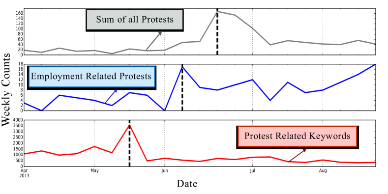
Figure 1: Illustrative example showing surrogate sources which could have led to an early detection of onset of 2013 Brazilian spring protests. (Top) Total protest counts in Brazil over Apr’13 to Aug’13 exhibiting a sharp increase around mid-June. (Middle) Employment and Wages related protests and (bottom) aggregated counts of a clusters of protest related keywords in Twitter.

Table 1: Comparison of state-of-the-art methods vs Hierarchical Quickest Change Detection

Desirable	Sequential	Window-	Bayesian	Relative	Hierarchical	HQCD
Properties	GLRT	Limited	Online	Density-	Bayesian	(This
	1963	GLRT	CPD	ratio	Analysis of	Paper)
	1995	1995	2007	Estimation	Change
		2010		(RuLSIF)	Point
				2013	Problems
					1992
Online	✓	✓	✓	✓		✓
Hierarchical					✓	✓
Bounded False
Alarm Rate /	✓	✓		✓		✓
Detection delay
Handles						✓
Non-IID data

Consider the evolution of the Brazilian Spring protests during mid June 2013 which are shown in terms of the total number of protests per week as in Fig. 1 (top panel). This uprising can be further analyzed by looking at individual categories of protests as shown in Fig. 1 (middle panel). As seen, during the Brazilian Spring there was a sharp increase in employment and wages related protests. It is noteworthy that similar observations can be made from Fig. 1 by observing the increase in Twitter activity for protest related keywords (bottom panel) such as “Aborto, Agravar, Central Dos Trabalhadores e Trabalhadoras Do Brasil” during early June. This example leads to the following important observations: there is potentially significant correlated information that can be leveraged to reduce detection delay, and identifying the informative data source(s) can help reduce the false positives. Thus, appropriate usage of such surrogate information can potentially lead to change detection with improved performance as well offer an interpretation behind the cause of the changepoint.

Motivated by the aforementioned observations, we propose Hierarchical Quickest Change Detection (HQCD), for online change detection across multiple sources, viz. target and surrogates. Typically, targets are sources of imminent interest (such as disease outbreaks or civil unrest); whereas surrogates (such as counts of the word ‘protesta’ in Twitter) by themselves are not of significant interest. Thus, HQCD  is aimed towards continuously utilizing both categories, but more focused on early (or quickest) detection of significant changes across the target sources. Traditional event (or change) detection approaches are not suitable for such problems. These are either a) offline approaches (Page, 1954; Wald, 1945; Shewhart, 1925; Carlin et al, 1992) using the entire data retrospectively - thus not applicable to real-time scenarios, or b) online detection approaches (Shiryaev, 1963; Siegmund and Venkatraman, 1995; Lai, 1995; Lai and Xing, 2010; Adams and MacKay, 2007; Liu et al, 2013) with primary focus on the target source of interest and do not utilize other correlated sources. Table 1 shows a comparison of HQCD and several state-of-the-art methods in terms of the desirable attributes.

The main contributions of this paper are:
$\bullet$ HQCD formalizes a hierarchical structure which in addition to the observed set of target sources (i.e., $S_{i}$’s), incorporates additional surrogates, denoted by $K_{j}$’s, and encodes propagation of change from surrogate to target sources.
$\bullet$ HQCD presents a specialized change detection metric that guarantees a maximum level of false alarm rate while reducing the detection delay in quickest detection framework. In addition, HQCD yields a natural methodology for analyzing the causality of change in a particular target source through a sequence of change propagations in other sources.
$\bullet$ HQCD presents a specialized sequential Monte Carlo based change detection framework that along with specialized change detection metrics enables hierarchical data to be analyzed in online fashion.
$\bullet$ We extensively test HQCD on both synthetic and real world data. We compare against state-of-the-art methods and illustrate the robustness of our methods and the usefulness of surrogates. We also present a detailed analysis of three protest uprisings using real world data and show that the uprising could have been predicted a few weeks in advance by incorporating surrogate data such as Twitter chatter. Moreover, we analyzed target-surrogate relationships and uncover important propagation patterns that led to such uprisings.

2 HQCD–Hierarchical Quickest Change Detection

We first provide a brief overview of classical QCD problem and then present the HQCD framework.

2.1 Quickest Change Detection (QCD)

Let us consider a data source $S$ changing over time and following different stochastic processes before and after an unknown time $\Gamma$ (changepoint). The task of QCD is to produce an estimate $\hat{\Gamma}=\gamma$ in an online setting (i.e., at time $t$, only $S_{1},\ldots,S_{t}$ is available). Figure 2 illustrates the two fundamental performance metrics related to this problem. In the figure, $\Gamma=t_{4}$ is the actual time-point when the changepoint happened. An early estimate such as $\gamma_{1}=t_{1}$ in the figure leads to a false alarm, where another estimate, such as $\gamma_{2}=t_{6}$ leads to an ‘additive delay’ of $\gamma_{2}-\Gamma=t_{6}-t_{4}$. The goal of QCD is to design an online detection strategy which minimizes the expected additive detection delay (EADD) while not exceeding a maximum pre-specified probability of false alarm (PFA). QCD has been studied in various contexts. Some of the foremost methods have considered i.i.d. distributions with known (or unknown) parameters before and after unknown changepoints (Veeravalli and Banerjee, 2013). Some of the more popular methods have used CUSUM (cumulative sum of likelihood) based tests while more general approaches are adapted in GLRT (generalized likelihood ratio test) based methods (Dessein and Cont, 2013).

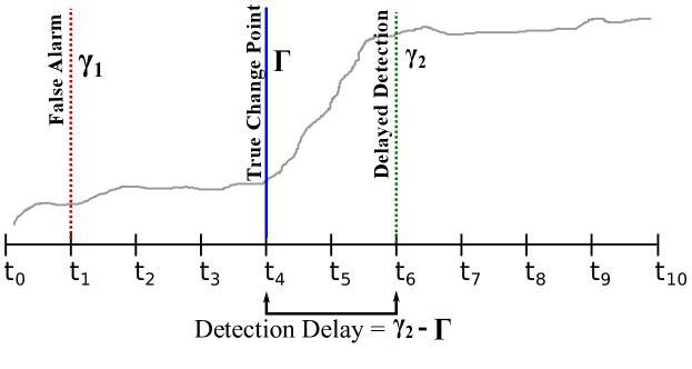
Figure 2: Illustration of Quickest Change Detection (QCD): blue colored line represents the actual changepoint at time $\Gamma=t_{4}$. (a) declaring a change at $\gamma_{1}$ leads to a false alarm, whereas (b) declaring the change at $\gamma_{2}$ leads to detection delay. QCD can strike a tradeoff between false alarm and detection delay.

2.2 Changepoint detection in Hierarchical Data

We next present our approach to generalize QCD to a hierarchical setting. We first describe a generic hierarchical model and then propose the QCD statistics for such models in Section 2.2.2. For computational feasibility, we present a bounded approximate of the same and our multilevel changepoint algorithm in Section 2.2.3.

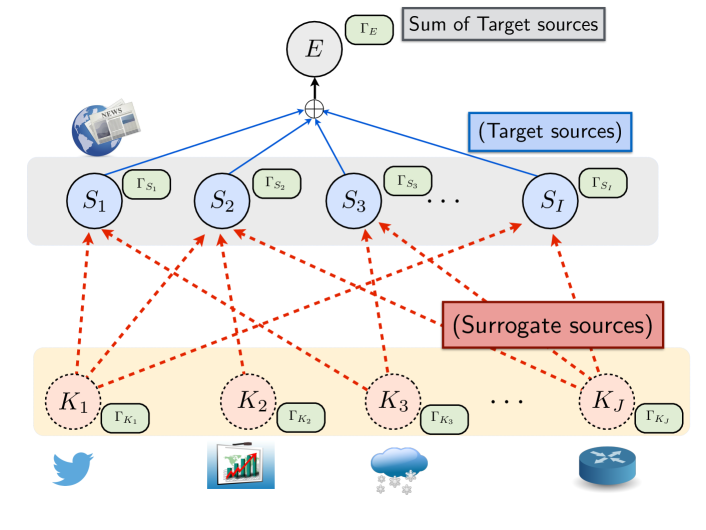
Figure 3: Generative process for HQCD. As an example consider civil unrest protests. In the framework, different protest types (such as Education- and Housing-related protests) form the targets denoted by $S_{i}$’s. The total number of protests will be denoted by the top-most variable $E$. Finally, the set of surrogates, such as counts of Twitter keywords, stock price data, weather data, network usage data etc. are denoted by $K_{j}$’s.

2.2.1 Generic Hierarchical Model

Let us consider $\bar{\mathbf{S}}^{(T)}$, a set of $I$ correlated temporal sequences $\{S_{1}^{(T)},S_{2}^{(T)},\dots S_{I}^{(T)}\}$ where, $S_{i}^{(T)}$ represents the $i^{th}$ target data sequence $S_{i}^{(T)}=\left[s_{i}(1),s_{i}(2),\dots,s_{i}(T)\right]$ for $i=1,\ldots,I$, collected up and until some time $T$. The cumulative sum of the target sources $S_{i}$’s at time $t$ is given by $E(t)$, i.e., $E(t)=\sum_{i=1}^{I}s_{i}(t)$. Concurrent to target sources, we also observe a set of $J$ surrogate sources, $\bar{\mathbf{K}}^{(T)}=\{K_{1}^{(T)},K_{2}^{(T)},\dots,K_{J}^{(T)}\}$, where $K_{j}^{(T)}=\left[k_{j}(1),k_{j}(2),\dots,k_{j}(T)\right]$, for $j=1,\ldots,J$, which may either have a causal or effectual relationship with the target source set $\bar{\mathbf{S}}^{(T)}$ (see Figure 3). We assume that targets and surrogates follow a stochastic Markov process as follows:

$$P(\bar{\mathbf{S}}^{(T)},\bar{\mathbf{K}}^{(T)})= P(S_{1}^{(T)},\ldots,S_{I}^{(T)},K_{1}^{(T)},\ldots,K_{J}^{(T)})$$

$$= \prod_{t=1}^{T}\Bigg{\{}\prod_{j=1}^{J}P_{t}^{\phi^{K}_{j}}(K_{j}(t))\times\prod_{i=1}^{I}P_{t}^{\phi^{S}_{i}}\left(S_{i}(t)|\bar{\mathbf{S}}^{(t-1)},\bar{\mathbf{K}}^{(t-1)}\right)\Bigg{\}}.$$

The binary variables $\phi^{K}_{j},\phi^{S}_{i}\in\{0,1\}$ capture the notion of significant changes in events through changes in distribution of the generative process as follows: if the surrogate source $K_{j}$ undergoes a change in distribution at some time $t$, then, $\phi^{K}_{j}$ changes from $0$ to $1$. In other words, $P_{t}^{0}(K_{j})$ (respectively $P_{t}^{1}(K_{j})$) denotes the pre-change (post-change) distribution of the $j$th surrogate source. Similarly, if the target source $S_{i}$ undergoes a change in distribution at some time $t$, then $\phi^{S}_{i}$ changes from $0$ to $1$. In other words, $P_{t}^{0}(S_{i}|\cdot)$ (respectively $P_{t}^{1}(S_{i}|\cdot)$) denotes the pre-change (post-change) conditional distribution of the $j$th target data source. We denote $\Gamma_{K_{j}}$ (respectively $\Gamma_{S_{i}}$) as the random variable denoting the time at which $\phi^{K}_{j}$ (respectively, $\phi^{S}_{i}$) changes from $0$ to $1$. Finally, we write $\bar{\mathbf{\Gamma}}_{\bar{\mathbf{K}}}=(\Gamma_{K_{1}},\ldots,\Gamma_{K_{J}})$, and $\bar{\mathbf{\Gamma}}_{\bar{\mathbf{S}}}=(\Gamma_{S_{1}},\ldots,\Gamma_{S_{I}})$ as the collective sets of changepoints in the surrogate and target sources, respectively. Finally, denote $\Gamma_{E}$ as the changepoint random variable for the top layer, $E$, which represents the sum total of all target sources.

2.2.2 From QCD to HQCD

We extend the concepts of QCD presented in Section 2.1 to multilevel setting by formalizing the problem as the earliest detection of the set of all $(J+I+1)$ changepoints, i.e., $\bar{\mathbf{\Gamma}}=\{\bar{\mathbf{\Gamma}}_{\bar{\mathbf{K}}},\bar{\mathbf{\Gamma}}_{\bar{\mathbf{S}}},\Gamma_{E}\}$ having observed the target and surrogate sources i.e. $\left(\bar{\mathbf{S}}^{(T)},\bar{\mathbf{K}}^{(T)}\right)$. Let $\bar{\mathbf{\gamma}}=\{\bar{\mathbf{\gamma}}_{\bar{\mathbf{K}}},\bar{\mathbf{\gamma}}_{\bar{\mathbf{S}}},\gamma_{E}\}$ be the $(J+I+1)$ vector of decision variables for the changepoints. To measure detection performance, we define the following two novel performance criteria:

Multi-Level Probability-of-False-Alarm (ML-PFA):

$$\text{ML-PFA}(\bar{\mathbf{\gamma}})=\mathbb{P}\left(\bar{\mathbf{\gamma}}\preceq\bar{\mathbf{\Gamma}}\right),$$ (1)

where for any two $N$ length vectors $a\preceq b$, the notation implies $a_{i}\leq b_{i}$, for $i=1,\ldots,N$. For instance, consider the example of $I=1$ target, and $J=1$ surrogate. Then $\bar{\mathbf{\Gamma}}=(\Gamma_{K_{1}},\Gamma_{S_{1}})$ and $\gamma=(\gamma_{K_{1}},\gamma_{S_{1}})$, and the probability of multi-level false alarm is given by $\text{ML-PFA}(\gamma)=\mathbb{P}(\gamma_{K_{1}}\leq\Gamma_{K_{1}},\gamma_{S_{1}}\leq\Gamma_{S_{1}})$. This definition of ML-PFA declares a false alarm only if all the $(J+I+1)$ change decision variables are smaller than the true changepoints.

Expected Additive Detection Delay (EADD):

$$\small\text{EADD}(\gamma)=\mathbb{E}\left(|\gamma-\bar{\mathbf{\Gamma}}|_{1}\right)=\underbrace{\sum_{j=1}^{J}\mathbb{E}(|\gamma_{K_{j}}-\Gamma_{K_{j}}|)}_{\text{Surrogate layer delay}}+\underbrace{\sum_{i=1}^{I}\mathbb{E}(|\gamma_{S_{i}}-\Gamma_{S_{i}}|)}_{\text{Target layer delay}}+\underbrace{\mathbb{E}|\gamma_{E}-\Gamma_{E}|}_{\text{Top layer delay}}$$ (2)

Given the observations, i.e., all target and surrogate sources $(\bar{\mathbf{S}}^{(T)},\bar{\mathbf{K}}^{(T)})$ till time $T$ governed by unknown changepoints $\bar{\mathbf{\Gamma}}$, we aim to make an optimal decision $\gamma$ about these changepoints under the following criterion

$$\gamma^{*}(\alpha)=\mbox{ arg}\min\limits_{\gamma}\text{ EADD}(\gamma)\hskip 15.0pt\text{ s.t. }\text{ML-PFA}(\gamma)\leq\alpha.$$ (3)

In other words, $\gamma^{*}(\alpha)$ is the optimal change decision vector which minimizes the EADD while guaranteeing that the ML-PFA is no more than a tolerable threshold $\alpha$. We note that the above optimal test is challenging to implement for real-world data sets due to following issues: a) it requires the knowledge of pre- and post- change distributions (for all sources) and the distribution of the changepoint random vector $\bar{\mathbf{\Gamma}}$, b) unlike single source QCD, finding the optimal $\gamma^{*}(\alpha)$ requires a multi-dimensional search over multiple sources, making it computationally expensive, and c) it does not discriminate between false alarms across different sources. For instance, declaring false alarm at a target source (such as premature declaration of the onset of protests or disease outbreaks) must be penalized more in comparison to declaring false alarm at a surrogate source (such as incorrectly declaring rise in Twitter activity).

2.2.3 Bounded approximation of HQCD

We can circumvent the problem (b) of the original definition of ML-PFA as given in equation 1 by upper bounding it in Theorem 2.1.

Theorem 2.1 (Modified-PFA).

Let $\bar{\mathbf{\gamma}}=\{\bar{\mathbf{\gamma_{S}}},\bar{\mathbf{\gamma_{K}}},\gamma_{E}\}$ be the a set of estimates about true changepoint for targets, surrogates and sum-of-targets, respectively. Then under the condition of greater importance to accurate target layer detections, ML-PFA (see 1) is upper-bounded by Modified-PFA, where:

$$\begin{array}[]{l}\small\text{Modified-PFA}(\gamma)\triangleq I\times\max\limits_{i}\mathbb{P}(\gamma_{S_{i}}\leq\Gamma_{S_{i}})+\min\limits_{j}\mathbb{P}(\gamma_{K_{j}}\leq\Gamma_{K_{j}})+\mathbb{P}(\gamma_{E}\leq\Gamma_{E})\end{array}$$ (4)

Proof.

We can prove the upper bound of ML-PFA with the following reductions:

$$\begin{array}[]{lcl}\text{ML-PFA}(\gamma)&=&\mathbb{P}(\gamma\preceq\Gamma)\\ &=&\mathbb{P}(\gamma_{\bar{\mathbf{S}}}\preceq\Gamma_{\bar{\mathbf{S}}},\gamma_{\bar{\mathbf{K}}}\preceq\Gamma_{\bar{\mathbf{K}}},\gamma_{E}\leq\Gamma_{E})\\ &\overset{(a)}{\leq}&\mathbb{P}(\gamma_{\bar{\mathbf{S}}}\preceq\Gamma_{\bar{\mathbf{S}}})+\mathbb{P}(\gamma_{\bar{\mathbf{K}}}\preceq\Gamma_{\bar{\mathbf{K}}})+\mathbb{P}(\gamma_{E}\leq\Gamma_{E})\\ &\overset{(b)}{\leq}&\sum_{i=1}^{I}\mathbb{P}(\gamma_{S_{i}}\leq\Gamma_{S_{i}})+\mathbb{P}(\gamma_{\bar{\mathbf{K}}}\preceq\Gamma_{\bar{\mathbf{K}}})+\mathbb{P}(\gamma_{E}\leq\Gamma_{E})\\ &\leq&I\times\max\limits_{i}\mathbb{P}(\gamma_{S_{i}}\leq\Gamma_{S_{i}})+\mathbb{P}(\gamma_{\bar{\mathbf{K}}}\preceq\Gamma_{\bar{\mathbf{K}}})+\mathbb{P}(\gamma_{E}\leq\Gamma_{E})\\ &\overset{(c)}{\leq}&I\times\max\limits_{i}\mathbb{P}(\gamma_{S_{i}}\leq\Gamma_{S_{i}})+\min\limits_{j}\mathbb{P}(\gamma_{K_{j}}\leq\Gamma_{K_{j}})+\mathbb{P}(\gamma_{E}\leq\Gamma_{E}),\end{array}$$ (5)

where $(a)$ and $(b)$ follows from the union bound on probability and $(c)$ follows from the fact that the joint probability of a set of events is less than the probability of any one event, i.e., $\mathbb{P}(\gamma_{\bar{\mathbf{K}}}\preceq\Gamma_{\bar{\mathbf{K}}})\leq\mathbb{P}(\gamma_{K_{j}}\leq\Gamma_{K_{j}})$, for any $j=1,\ldots,J$, and then taking the minimum over all $j$. The resulting upper bound in (5) leads to the basis of the modification of the multi-level PFA:

$$\text{Modified-PFA}(\gamma)\triangleq I\times\max\limits_{i}\mathbb{P}(\gamma_{S_{i}}\leq\Gamma_{S_{i}})\\ +\min\limits_{j}\mathbb{P}(\gamma_{K_{j}}\leq\Gamma_{K_{j}})+\mathbb{P}(\gamma_{E}\leq\Gamma_{E})$$

∎

Modified-PFA expression leads to intuitive interpretations as follows: (i) as false alarms at targets can have a higher impact, it is desirable to keep the worst case PFA across these to be the smallest, or equivalently, $\max_{i}\mathbb{P}(\gamma_{S_{i}}\leq\Gamma_{S_{i}})$ should be minimized. (ii) false alarms at surrogates are not as impactful and we can declare a false alarm if all of the surrogate level detection(s) are unreliable, or equivalently, $\min_{j}\mathbb{P}(\gamma_{K_{j}}\leq\Gamma_{K_{j}})$ needs to be minimized. (iii) notably, the above modification leads to a low-complexity change detection approach across multiple sources by locally optimal detection strategies avoiding a multi-dimensional search.

Based on Modified-PFA, we next present a compact test suite to declare changes at pre-specified levels of maximum PFA as given in Theorem 2.2 and incorporate specificity issues pointed out in problem (c) of the original formulation of PFA.

Theorem 2.2 (Multi-level Change Detection).

Let $\Gamma_{S_{i}}$ be the true change point random variable for the $i$th target source, $S_{i}$. Let $\Gamma_{K_{j}}$ and $\Gamma_{E}$ represent the same for the $j$th surrogate and the sum-of-targets, respectively. Let the data observed till time $T$ be $D^{(T)}\triangleq\left(\bar{\mathbf{S}}^{(T)},\bar{\mathbf{K}}^{(T)}\right)$ and $P(\bar{\mathbf{\Gamma}}|D^{(T)})$ denote the estimate of the conditional distribution (see Section 3.2). Then, if $\alpha_{i},\beta_{j},\lambda$ represent the PFA thresholds for the $S_{i},K_{j},E$, the changepoint tests can be given as:

$$\gamma_{S_{i}}(\alpha_{i}) =\text{inf}\left\{n:\text{TS}_{S_{i}}(D^{(T)})\geq\frac{\alpha_{i}}{1+\alpha_{i}}\right\},i=1,\ldots,I$$ (6a)

$$\gamma_{K_{j}}(\beta_{j}) =\text{inf}\left\{n:\text{TS}_{K_{j}}(D^{(T)})\geq\frac{\beta_{j}}{1+\beta_{j}}\right\},j=1,\ldots,J$$ (6b)

$$\gamma_{E}(\lambda) =\text{inf}\left\{n:\text{TS}_{E}(D^{(T)})\geq\frac{\lambda}{1+\lambda}\right\},$$ (6c)

where $\text{TS}_{X}(D^{(T)})=\mathbb{P}(\Gamma_{X}\leq n|D^{(T)})$ is the test statistic (TS) for a source $X$.

Proof.

In quickest change detection, our goal at time $T$ is to decide if a change should be declared for some $n\leq T$ for a particular data source. To this end, we can use the following change detection test

$$\gamma_{S_{i}}(\alpha_{i})=\text{inf}\left\{n:\log\left(\frac{P\left(\Gamma_{S_{i}}\leq n|D^{(T)}\right)}{P\Big{(}\Gamma_{S_{i}}>n|D^{(T)}\Big{)}}\right)\geq\log(\alpha_{i})\right\},$$

which is equivalent to the following test:

$$\gamma_{S_{i}}(\alpha_{i})=\text{inf}\left\{n:P\left(\Gamma_{S_{i}}\leq n|D^{(T)}\right)\geq\frac{\alpha_{i}}{1+\alpha_{i}}\right\}.$$ (7)

Intuitively, the above test declares the change for the $i$th target source $S_{i}$ at the smallest time $n$ for which the test statistic (i.e., posterior probability of the change point random variable being less than $n$) exceeds a threshold. The probability of false alarm for the above test can be bounded in terms of the threshold $\alpha_{i}$ as:

$$\begin{array}[]{lcl}\mathbb{P}(\gamma_{S_{i}}\leq\Gamma_{S_{i}})&=&\sum_{D^{(T)}}\sum_{n}\mathbb{P}(D^{(T)},\gamma_{S_{i}}=n)\mathbb{P}(\Gamma_{S_{i}}>n|D^{(T)},\gamma_{S_{i}}=n)\\ &\overset{(d)}{\leq}&\underbrace{\sum_{D^{(T)}}\sum_{n}\mathbb{P}(D^{(T)},\gamma_{S_{i}}=n)}_{=1}\left(\frac{1}{1+\alpha_{i}}\right)\\ &=&\frac{1}{1+\alpha_{i}},\end{array}$$ (8)

where $(d)$ follows from the fact that given the observed data and the event, $\gamma_{S_{i}}=n$, i.e., the change is declared at $n$, then it follows from (equation 7) that

$$\mathbb{P}(\Gamma_{S_{i}}>n|D^{(T)},\gamma_{S_{i}}=n)\leq 1/(1+\alpha_{i})$$

Let us denote the test statistic (TS) for a data source $X$ as:

$$\text{TS}_{X}(D^{(T)})=\mathbb{P}(\Gamma_{X}\leq n|D^{(T)})$$

Then, then the multi-level change detection test is:

$$\gamma_{S_{i}}(\alpha_{i}) =\text{inf}\{n:\text{TS}_{S_{i}}(D^{(T)})\geq\frac{\alpha_{i}}{1+\alpha_{i}}\},i=1,\ldots,I$$

$$\gamma_{K_{j}}(\beta_{j}) =\text{inf}\{n:\text{TS}_{K_{j}}(D^{(T)})\geq\frac{\beta_{j}}{1+\beta_{j}}\},j=1,\ldots,J$$

$$\gamma_{E}(\lambda) =\text{inf}\{n:\text{TS}_{E}(D^{(T)})\geq\frac{\lambda}{1+\lambda}\}$$

∎

From Theorem 2.2, we can infer the following boundedness property of Modified-PFA as expressed in the following Lemma.

Lemma 2.3.

If we define $\alpha\overset{\Delta}{=}\min_{i}(\alpha_{i})$ and $\beta\overset{\Delta}{=}\max_{j}(\beta_{j})$, then Modified-PFA in equation 4 can be bounded as:

$$\text{Modified-PFA}(\gamma)\leq{I\times\frac{1}{1+\alpha}}+{\frac{1}{1+\beta}}+{\frac{1}{1+\lambda}}$$ (10)

Input : At time $T$, Target and Surrogate Sources $D^{(T)}=\left(S^{(T)},K^{(T)}\right)$

Parameters : PFA threshold for targets ($\alpha$), surrogates ($\beta$), and sum of targets ($\lambda$)

Output : Changepoint Decisions $\bar{\mathbf{\gamma_{S}}},\bar{\mathbf{\gamma_{K}}},{\gamma_{E}}$ at each timepoint $T$

1 for each $T$  do

2       Update joint posterior$P(\Gamma_{K},\Gamma_{S},\Gamma_{E}|D^{(T)})$

       // target change detection

3       for $i\leftarrow 1$ to $I$ do

4             Compute target marginal $P(\Gamma_{S_{i}}|D^{(T)})$

5             Find $\gamma_{S_{i}}(\alpha)$ using 6a

6            

7      $\bar{\mathbf{\gamma_{S}}}\leftarrow\{\gamma_{S_{1}}(\alpha),\dots,\gamma_{S_{I}}(\alpha)\}$

       // surrogate change detection

8       for $j\leftarrow 1$ to $J$ do

9             Compute surrogate marginal $P(\Gamma_{K_{j}}|D^{(T)})$

10             Find $\gamma_{K_{j}}(\beta)$ using 6a

11            

12      $\bar{\mathbf{\gamma_{K}}}\leftarrow\{\gamma_{K_{1}}(\beta),\dots,\gamma_{K_{J}}(\beta)\}$

       // sum-of-targets change detection

13       Compute sum-of-targets marginal $P(\Gamma_{E}|D^{(T)})$

14       Find $\gamma_{E}(\lambda)$ using 6c

15       Return Decision $\bar{\mathbf{\gamma_{S}}},\bar{\mathbf{\gamma_{K}}},{\gamma_{E}(\lambda)}$ at $T$

16      

Algorithm 1 HQCD  Multi-level Change Point Detection Algorithm

3 HQCD for Protest Detection via Surrogates

(a)

(b)

Figure 4: Histogram fit of (a) surrogate source (Twitter keyword counts) and (b) target source (Number of protests of different categories), for various temporal windows, under i.i.d. assumptions. These assumptions lead to satisfactory distribution fit, at a batch level, for both sources. The top-most row corresponds to the period before the Brazilian spring (pre 2013-05-25), the second row is for the period 2013-05-25 to 2013-10-20, and the third is for the period after 2013-10-20. The last row shows the fit for the entire period. These temporal fits are indicative of significant changes in distribution along the Brazilian Spring timeline, for both target and surrogates.

In this section we discuss the HQCD framework for early detection of protest uprisings via surrogate sources. Protests can happen in civil society for various reasons such as protests against fare hike or protests demanding more job opportunities. Such protests, especially major changes in protest base levels, are potentially interlinked. However explaining such interactions is a non-trivial process. Ramakrishnan et al (2014) found several social sources, especially Twitter chatter, to capture protest related information. We apply HQCD to find significant changes in protests concurrent to changes in Twitter chatter, such that detecting changes accurately are of primary importance in contrast to the chatters which can be influenced by a range of factors, including protests. In general, HQCD can be applied in similar events, such as disease outbreaks, to find significant changes in targets using information from noisy surrogates.

3.1 Hierarchical Model for Protest Count Data

For the case of protest uprisings, we first note that surrogate sources such as Twitter are in general noisy and involve a complex interplay of several factors - one of which could be protest uprisings. Furthermore, for protest uprisings, we are more concerned in using the surrogates (Twitter chatter) to help declare changes at target level (protest counts) than accurately identifying the changes in surrogates. Thus, without loss of generality, we model the surrogates as i.i.d. distributed variables. Figure 4) evaluates the i.i.d. assumptions, for both protest counts and Twitter chatter. Our results indicate that Log-normal is a reasonable fit for Twitter chatter.

Surrogate Sources: Formally, we assume that the $j^{th}$ surrogate source $K_{j}$ is generated i.i.d. from a distribution $f^{K}$ w.r.t to the associated changepoint $\Gamma_{K_{j}}$ as:

$$k_{j}(t)\overset{i.i.d}{\sim}\begin{cases}\begin{array}[]{lr}f^{K}(\phi^{K_{j}}_{0})&t\leq\Gamma_{K_{j}}\\ f^{K}(\phi^{K_{j}}_{1})&t>\Gamma_{K_{j}}\end{array}\end{cases}\vspace{-4pt}$$ (11)

where, $\phi^{K_{j}}_{0}$ and $\phi^{K_{j}}_{1}$ are the pre- and post-change parameters. Following our earlier discussion, we select $f^{K}$ as Log-normal (with location and scale parameters $\phi^{K_{j}}=\{c^{K_{j}},d^{K_{j}}\}$) for Twitter counts.

Target Sources: Target sources can in general be dependent on both the past values of targets as well as the surrogates. Here, we restrict the target source process to be a first order Markov process. Under this assumption, we formalize the $i^{th}$ target source $S_{i}$ to follow a Markov process $f^{S}_{t}$ w.r.t to its changepoint $\Gamma_{S_{i}}$ as:

$$s_{i}(t)\sim\begin{cases}\begin{array}[]{lr}f^{S}_{t}(\phi^{S_{i}}_{0}(t))&t\leq\Gamma_{S_{i}}\\ \vspace{1pt}f^{S}_{t}(\phi^{S_{i}}_{1}(t))&t>\Gamma_{S_{i}}\\ \end{array}\end{cases}$$ (12)

where, $\phi^{S_{i}}_{0}$ and $\phi^{S_{i}}_{1}$ are the pre- and post-change parameters of the process. Poisson process with dynamic rate parameters has been shown (Carlin et al, 1992) to be effective in specifying hierarchical count data w.r.t changepoints. Here, we model the rate parameters as a nested autoregressive process (Fokianos et al, 2009; Carlin et al, 1992) given as:

$$\begin{array}[]{lcl}\phi^{S_{i}}_{0/1}(t)&=&\phi^{S_{i}}_{0/1}(t-1)+\frac{A^{i}_{0/1}(t)}{|A^{i}_{0/1}(t)|}\dbinom{S(t-1)}{K(t-1)}+\mathcal{N}(0,\sigma_{S})\\ A^{i}_{0/1}(t)&=&A^{i}_{0/1}(t-1)+\mathcal{N}(0,\Sigma_{A^{i}})\end{array}$$ (13)

Here, $\phi_{0/1}^{S}(t)$ captures the latent rate and $\sigma_{S}$ denotes the error variance. $A_{0/1}^{i}(t)$ captures the variation due to the observed values of target and surrogates sources.

Changepoint Priors: Following our prior discussion, surrogate changepoints can be assumed to have an uninformative prior and we model $\Gamma_{K_{j}}$ via a memoryless arrival distribution (static probability of observing change given it hasn’t occurred earlier) as:

$$\Gamma_{K_{j}}\sim\text{Geom}(\rho_{K_{j}})\Rightarrow P(K_{j}=t|K_{j}\geq t)=\rho_{K_{j}}$$ (14)

Conversely, target changepoints can be influenced by surrogate changepoints as their generative process is dependent on the surrogates. Specifically, whenever we observe a changepoint in the surrogates, we assume that the base rate of changepoint for a target to increase for a certain period of time. Formally, target changepoint priors are assumed to follow a dynamic process as:

$$\Gamma_{S_{i}}\sim\text{Geom}(\rho_{S_{i}(t)})\vspace{-5pt}$$ (15)

$$\rho_{S_{i}}(t)=\rho_{S_{i}}+\sum\limits_{j}\mathcal{I}(\Gamma_{K_{j}}<t)\mu^{1}_{j}e^{-\mu^{2}_{j}(t-\Gamma_{K_{j}})}\vspace{-5pt}$$

where, $\mathcal{I}$ is the indicator function. $\rho_{S_{i}}$ represents the nominal base rate for the changepoint. It can be seen, a change in the $j$th surrogate source is modeled as an exponentially decaying ‘impulse’ of amplitude $\mu^{1}_{j}$. The summation of targets, $E(t)$ is known deterministically given $S_{i}(t)$. Moreover, given $S_{i}(t-1)$, $E(t)$ can be considered to be summation of independent Poisson processes following similar dynamics as equation 13 which is omitted due to limited space. Similarly, relationships for dependence of $\Gamma_{E}$ can be modeled to be dependent on $K$ similar to equation 15.

3.2 Changepoint Posterior Estimation

Algorithm 1 involves posterior estimation of the changepoints given the data at a particular time point. Earlier works have focused mainly on offline methods such as Gibbs Sampling (Carlin et al, 1992). Online posterior estimation for such problems have been studied extensively in the context of Sequential Bayesian Inference (Casella and Berger, 2002) such as Kalman filters (Kalman, 1960; Simon, 2010; Anderson, 2001) (Gaussian transitions) and Particle Filters (Del Moral, 1996; Pitt and Shephard, 1999; Doucet and Johansen, 2009). Recently, Chopin et al.  (Chopin et al, 2013) proposed a robust Particle Filter, SMC² which is ideally suited for fitting the parameters of the non-linear hierarchical model described in Section 3.1. In this section we formulate a Sequential Bayesian Algorithm that makes the HQCD tractable under real world constraints (see Figure 5).

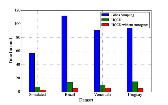
Figure 5: Computation time for one complete run of changepoint detection (in mins) on a 1.6 GHz quad core 8gb intel i5 processor: Gibbs sampling (Carlin et al, 1992) vs HQCD vs HQCD without surrogates. Gibbs sampling computation times are unsuitable for online detection.

To find the posterior $P\left(\bar{\mathbf{\Gamma}}_{S},\bar{\mathbf{\Gamma}}_{K},\Gamma_{E}|D^{(T)}\right)$ at any time $T$ using SMC² we first cast the model parameters and variables into the following three categories:

Observations $({y_{T}})$: In the context of SMC² these are the parameters that correspond to observed variables at each time point $T$. For HQCD we can model $y_{T}$ as:

$${y_{T}}\overset{\Delta}{=}\{S(T),K(T)\}$$ (16)

Hidden States $({x_{T}})$: SMC² estimates the observations based on interaction with hidden states which are dynamic, unobserved and is sufficient to describe $y_{T}$ at $T$. For HQCD, we can express $x_{T}$ as follows:

$${x_{T}}\overset{\Delta}{=}\{\bar{\mathbf{\Gamma}}_{S},\bar{\mathbf{\Gamma}}_{K},\Gamma_{E},\bar{\mathbf{\phi}}_{0/1}^{S}(T-1),\bar{\mathbf{\phi}}_{0/1}^{K},\vspace{-7pt}$$ (17)

$$\bar{\mathbf{\rho}}_{K}(T),\bar{\mathbf{\rho}}_{S}(T),\bar{\mathbf{A}}_{0/1},S(T-1),K(T-1)\}$$

Static Parameters $({\theta})$: Finally, SMC² also accommodates the concept of static parameters which do not change over time such as the base probabilities of changepoint $\bar{\mathbf{\rho_{S}}}$ and the noise matrix $\Sigma_{A}$ in HQCD. We can express $\theta$ as:

$$\vspace{-5pt}\theta\overset{\Delta}{=}\{\sigma_{S},\Sigma_{A},\bar{\mathbf{\rho_{S}}},\bar{\mathbf{\mu^{1}}},\bar{\mathbf{\mu^{2}}}\}$$ (18)

For a given set of such parameters, SMC² works by first generating $N_{\theta}$ samples of $\theta$ using the prior distribution $P(\theta)$. For each of these samples of $\theta$, SMC² samples $N_{X}$ samples of $x_{0}$ from its prior $P(x_{0}|\theta)$. Following standard practices, we use conjugate distributions (Casella and Berger, 2002) for the priors.

Input : At time $T$, $y_{T}$ as give in equation 16

Parameters : Prior distributions $P(\theta)$ and $P(x_{0}|\theta)$

Hyperparameters for $P(\theta)$ and $P(x_{0}|\theta)$

Output : joint posterior $P(\Gamma_{K},\Gamma_{S},\Gamma_{E}|D^{(T)})$

1 Define $x_{T}$ as give in equation 17

2 Define $\theta$ as give in equation 18

// Initialization

3 Sample $N_{\theta}$ number of $\theta_{q}$ using $P(\theta)$

4 Sample $N_{x}$ number of $x_{0_{q,r}}$ using $P(x_{0}|\theta_{q})$

Update weights $w(0)$

  // See Appendix

// Online Learning

5 for each $T$ do

       // State Updates

6       for each $q\in N_{\theta}$ do

7             for each $r\in N_{x}$ do

8                   Update States: $x_{T_{q,r}}$ from $x_{{T-1}_{q,r}}$

9                   Compute Importance weights $w_{q,r}(T)$

10                   Compute observation probability $P(y_{T}|y_{T-1},\theta_{q})$

11            

      // Incorporate observation at time $T$

12       Update Importance weight $w_{q,r}(T)\leftarrow w_{q,r}(T)P(y_{T}|y_{T-1},\theta_{q})$

       // test premature convergence

13       Test degeneracy conditions using effective sample size

14       if degeneracy then

             // markov kernel jumps

15             Update $x_{T_{q,r}}$ by multiplying a markov Kernel $\mathcal{K}_{T}$

             // recomputing weights

16             exchange $x_{T_{q,r}}$ and set $w_{q_{r}}\propto 1$

17            

      // Find joints

18       Return Update $P(\bar{\mathbf{\Gamma}}_{S},\bar{\mathbf{\Gamma}}_{K},\Gamma_{E}|D^{(T)})$ using equation 19

Algorithm 2 HQCD  Changepoint Posterior estimation via SMC²

At each time point $T$, the samples are perturbed using the model equations given in Section 3.1 and associated with weights $w$ to estimate the joint posteriors as:

$$\begin{array}[]{rcl}P(\theta,x_{T}|y_{T})&=&\sum\limits_{q=1}^{N_{\theta}}\sum\limits_{r=_{1}}^{N_{x}}w_{q,r}\delta(\theta,x_{T})\\ P\left(\bar{\mathbf{\Gamma}}_{S},\bar{\mathbf{\Gamma}}_{K},\Gamma_{E}\ |D^{(T)}\right)&\propto&\sum\limits_{q=1}^{N_{\theta}}\sum\limits_{r=_{1}}^{N_{x}}w_{q,r}\delta(\bar{\mathbf{\Gamma}}_{S},\bar{\mathbf{\Gamma}}_{K},\Gamma_{E})\end{array}$$ (19)

where, $\delta$ is the Kronecker-delta function. Algorithm 2 outlines the steps involved in this process. For more details on SMC² see Appendix.

4 Experiments

We present experimental results for both synthetic and real-world datasets, and compare HQCD against several state-of-the-art online change detection methods (see Table 1), specifically, GLRT (Siegmund and Venkatraman, 1995), W-GLRT (Lai and Xing, 2010), BOCPD (Adams and MacKay, 2007) and RuLSIF (Liu et al, 2013). To further analyze the effects of surrogates in detecting changepoints, we compare against HQCD without surrogates, where $K(t-1)$ is dropped from equation 13 and $\rho_{S_{i}(t)}$ is made static (i.e. independent of changepoints from surrogates) in equation 15.

Table 2: (Synthetic data) comparing true changepoint ($\Gamma$) for targets against detected changepoint ($\gamma$) by HQCD against state-of-the-art methods for false alarm (FA) and additive detection delay (ADD). Each row represent a target and best detected changepoint is shown in bold whereas false alarms are shown in red.

	True	GLRT		WGLRT		BOCPD		RuLSIF		HQCD		HQCD w/o surr.
	$\Gamma$	$\gamma$	ADD	$\gamma$	ADD	$\gamma$	ADD	$\gamma$	ADD	$\gamma$	ADD	$\gamma$	ADD
$S_{1}$	29	7	–	10	–	13		36	7	33	4	32	3
$S_{2}$	6	11	5	14	8	16	10	28	22	8	2	9	3
$S_{3}$	24	7	–	16	–	15		29	5	22	-	26	2
$S_{4}$	26	5	–	11	–	11		38	12	27	1	31	5
$S_{5}$	47	40	–	15	–	8		26	-	50	3	55	8

Figure 6: Comparison of HQCD against state-of-the-art on simulated target sources. X-axis represents time and Y-axis represents actual value. Solid blue lines refer to the true changepoint, solid green refers to the ones detected by HQCD and brown refers to HQCD without surrogates. Dashed red, magenta, purple and gold lines refer to changepoints detected by RuLSIF, WGLRT, BOCPD and GLRT, respectively. HQCD shows better detection for most targets with low overall detection delay and false alarms.

4.1 Synthetic Data

In this section, we validate against synthetic datasets with known changepoint parameters. For this, we pick 5 targets ($I=5$) and 10 surrogates ($J=10$). The surrogates were generated from i.i.d. Log-normal distributions (see equation 11) while the targets were generated using Poisson process (see equation 12). The changepoints for surrogates were sampled from a fixed Gamma distribution (see 14) while the associated changepoints for target sources were simulated via equation 15.

4.1.1 Comparisons with state-of-the-art

As true changepoints are known for the synthetic dataset, we can compare HQCD against the state-of-the-art methods for the detected changepoint as shown in Figure 6. Table 2 presents the results in terms of the false alarm (FA) and additive detection delay (ADD). From the table, we can see that HQCD is able to detect the changepoints with fewer false alarms. Also HQCD has the lowest delay across all methods for all targets except Target-1 for which HQCD without surrogates achieved better delay indicating the surrogates are not informative for this target source.

4.1.2 Usefulness of Surrogates

Our comparisons with the state-of-the-art shows significant improvements that were achieved by HQCD, both in terms of FA and ADD and showcase the importance of systematically admitting surrogate information to attain a quicker change detection with low false alarm. We compare HQCD with surrogates against HQCD without surrogates (Table 2) and find that admitting surrogates significantly improves average delay ($2.5$ compared to $4.2$). We also plot the average false alarm rate against the detection delay in Figure 7 and find that HQCD results are in general the ones with the best tradeoff between FA and ADD.

Figure 7: False Alarm vs Delay trade-off for different methods. HQCD shows the best trade-off.

(a) Civil Unrest Protests

(b) Twitter chatter

Figure 8: Illustration of civil unrest data: (a) shows an example where relevant news articles (top) are scanned to produce an annotated dataset of protest activities. (b) Geo-fenced Twitter data(top). Twitter chatter can uncover various socio-political factors, some of which could be civil unrest events(bottom).

4.2 Analysis of Protest Uprisings

In real-life scenarios, the true changepoint is typically unknown. One representative example could be seen w.r.t. the onset of major civil unrest related protests and uprisings. We present a detailed analysis of three major uprisings: (i) in Brazil around mid 2013 (often termed as the Brazilian Spring), (ii) in Venezuela around early 2014 and, (iii) in Uruguay around late 2013. We first describe the data collection procedure (Figure 8) and followup with a comparative analysis of detected changepoints.

Weekly counts of civil unrest events from Nov. 2012 to Dec. 2014 were obtained as part of a database of discrete unrest events (Gold Standard Report - GSR) prepared by human analysts by parsing news articles for civil unrest content. Among other annotations, the GSR also classifies each event to one of 6 possible event types based on the reason (‘why’) behind the protest. Each of these event types such as a) Employment and Wages, b) Housing, c) Energy and Resources, d) Other government, e) Other economic and f) Other, bears certain societal importance. We treat the weekly counts of each of these event-types as target sources ($S$) and the sum total of all protests for a week as the sum-of-targets ($E$). We also collected geo-fenced tweets for each country over the same time-period. We used a human-annotated dictionary of 962 such keywords/phrases that contains several identifiers of protest in the languages spoken in the countries of interest (similar to Ramakrishnan et.al. (Ramakrishnan et al, 2014)). As most of these keywords could have similar trends, we cluster them using k-means into 30 clusters (i.e., we have $J=30$ surrogates). To account for scaling effects while preserving temporal coherence, each keyword time-series was normalized to zero-mean and unit variance.

Table 3: (Protest uprisings) Comparison of HQCD vs state-of-the-art with respect to detected changepoints

	Event-Type	GLRT	WGLRT	BOCPD	RuLSIF	HQCD
		$\gamma$	$\gamma$	$\gamma$	$\gamma$	$\gamma$	EADD
Brazil	Employment & Wages	02/10	03/17	06/16	05/26	08/18	4
	Energy & Resources	02/10	03/17	06/09	05/19	06/02	6
	Housing	03/24	03/31	07/28	05/19	06/16	8
	Other Economic	03/24	03/24	06/23	05/19	06/30	5
	Other Government	02/17	06/23	04/07	05/19	06/16	4
	Other	03/03	03/17	06/30	05/19	06/23	6
	All	02/17	04/28	05/19	06/16	06/16	8
Venezuela	Employment & Wages	01/14	01/13	01/28	01/25	01/27	3
	Energy & Resources	01/20	01/11	02/28	01/20	02/24	7
	Housing	-	-	-	-	-	-
	Other Economic	01/31	01/31	01/28	-	01/27	9
	Other Government	01/22	01/11	02/03	01/20	02/10	4
	Other	01/14	01/12	01/25	01/30	01/24	5
	All	01/26	01/11	01/30	01/20	02/12	3
Uruguay	Employment & Wages	12/06	12/08	12/13	12/03	12/10	3
	Energy & Resources	12/04	12/05	12/10	-	12/09	4
	Housing	12/21	12/06	11/30	-	11/28	2
	Other Economic	12/20	12/06	-	-	11/26	2
	Other Government	11/25	12/05	12/16	11/29	12/15	3
	Other	12/05	12/09	12/03	-	01/14	10
	All	12/05	12/09	12/03	11/29	12/10	3

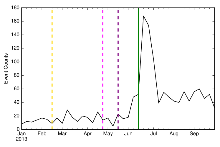
(a) Brazil Total Protests

(b) Venezuela Total Protests

(c) Uruguay Total Protests

Figure 9: Comparison of detected changepoints at the sum-of-targets (all Protests). HQCD detections are shown in solid green while those from the state-of-the-art methods i.e. RuLSIF (red), WGLRT (magenta), BOCPD (purple) and GLRT (gold) are shown with dashed lines. HQCD detection is the closest to the traditional start date of Mass Protests in the three countries studied .

(a) Brazil Subtypes

(b) Venezuela Subtypes

(c) Uruguay Subtypes

Figure 10: Comparison of detected changepoints at the target sources (Protest types) HQCD detections are shown in solid green while those from the state-of-the-art methods i.e. RuLSIF (red), WGLRT (magenta), BOCPD (purple) and GLRT (gold) are shown with dashed lines.

4.2.1 Changepoint Across layers

We show the changepoints detected by HQCD (bold green) and the state-of-the-art methods (dashed lines) for the sum-of-all protests in Figure 9 and individual protest types in Figure 10. We can observe that HQCD, which uses the surrogate information sources and exploits the hierarchical structure, finds indicators of changes which are visually better as well as more aligned to the dates of major events (See demo at https://prithwi.github.io/hqcd_supplementary). In contrast, the state-of-the-art methods can be argued to show significantly high false alarm rate. For such real world data sources, the notion of a true changepoint is difficult to ascertain, we can instead consider for example the onset of Brazilian spring protests (2013-06-01) as an underlying changepoint to compare at the sum-of-targets and interpret notions of false alarm. Table 3 tabulates these inferences for the targets as well as the sum-of-targets. Although, a true changepoint is unknown, we note that for HQCD, the expected additive detection delay (EADD) can be estimated according to equation 2 (from $P(\bar{\mathbf{\Gamma}}|D^{(T)})$ in Algorithm 2).

(a) Influence of lagged targets on current targets

(b) Influence of lagged surrogates on current targets

Figure 11: (Brazilian Spring) Heatmap of changepoint influences of targets on targets (a); and surrogates on targets (b). Darker (lighter) shades indicate higher (lesser) changepoint influence. (a) shows presence of strong off-diagonal elements indicating strong cross-target changepoint information. (b) shows a mixture of uninformative and informative surrogates.

4.2.2 Changepoint influence analysis

The experiments presented in the previous section can be further analyzed to ascertain the nature of progression of significant events that lead to a protest. Here we present our analysis for Brazilian Spring. As a preliminary step, from Table 3 we can see that the detected changepoints for Brazil reveal an interesting progression - significant changes in Energy related unrests (06/02) propagated to Housing/Other Govt. unrests (06/16) and culminated in mass Employment related unrests (08/18). Interestingly, we can analyze the fitted parameters of the weight vector $A^{i}_{0/1}$ of the rate updates (see 13) to quantize the changepoint influence of a source (target/surrogate) at time $T-1$ to time $T$. For each target $S_{i}$, we can compute the average value of the weight vector component of each target/surrogate separately. Let $h_{0}$ and $h_{1}$ denote these averages for one such source. Effectively, $h_{0}$ then measures the effect of the source at time $t-1$ on $S_{i}$ at $t$ before change while $h_{1}$ captures the same post change. Their percentage relative change can then be used as a measure of the changepoint influence of a particular target/surrogate source on $S_{i}$. We plot a heatmap of these percentages in Figure 11 for both targets and surrogates, separately. From Figure 11(a), we can see that ‘Other Economic’ and ’Employment’ related protests had strong influences from ‘Housing’ related protests. Furthermore, from Figure 11(b) we can see ‘Housing’ and ‘Employment’ related protests were influenced by similar Twitter chatter clusters (cluster-01 and cluster-26) - indicating that the interaction between these protest subtypes can be inferred from social domain. Conversely, ‘Housing’ and ‘Other Economic’ related protests are only weakly correlated through Twitter chatters - thus exhibiting the robustness of HQCD which can still detect interactions between targets when surrogates fail to explain the same. In general, for a particular target we can see linked pre-cursors in other targets (strong off-diagonal elements in Figure 11(a)) and highly specific informative surrogates (few strong cells for a row in Figure 11(b)).

5 Conclusion

We have presented HQCD, a framework for online change detection in multiple data sources which can augment additional surrogate information sources in a hierarchical manner. Key properties of our framework are the following a) it is computationally inexpensive requiring a search over local change points (for each data layer) making it applicable for a large number of data/surrogate sources, b) the change detection algorithms are readily tunable to account for different false alarm requirements at different data layers, and c) it provides a systematic approach to integrate surrogate information for the same. As shown through a variety of experiments on both synthetic and real world data sets, the proposed approach uncovers interesting relationships and significantly outperforms state-of-the-art methods which do not account for surrogate information both in terms of event detection reliability (probability of false alarm) as well as the delay in detection.

Supporting Information A demo of HQCD and the datasets used in this paper can be found in https://prithwi.github.io/hqcd_supplementary. Attached appendix provides additional details on SMC².

Acknowledgements Supported by the Intelligence Advanced Research Projects Activity (IARPA) via Department of Interior National Business Center (DoI/NBC) contract number D12PC000337, the US Government is authorized to reproduce and distribute reprints of this work for Governmental purposes notwithstanding any copyright annotation thereon. Disclaimer: The views and conclusions contained herein are those of the authors and should not be interpreted as necessarily representing the official policies or endorsements, either expressed or implied, of IARPA, DoI/NBC, or the US Government.

Appendix A Sequential Bayesian Inference

Consider a stochastic process where an observed temporal data sequence $\bar{\mathbf{y}}=\{y_{1},y_{2},\ldots,y_{t}\}$ depends on unobserved latent states $\bar{\mathbf{x}}=\{x_{1},x_{2},\ldots,x_{t}\}$ such that the following formulation holds:

$$\begin{array}[]{rcl}P(y_{t}|y_{1:t-1},x_{1:t},\theta)&=&f_{\theta}(y_{t}|x_{t})\\ P(x_{t}|x_{1:t-1},\theta)&=&g_{\theta}(x_{t}|x_{t-1})\\ P(x_{1}|\theta)&=&\mu_{\theta}(x_{1})\\ \Pi_{0}(\theta)&=&P(\theta)\\ \end{array}$$ (20)

i.e. $y_{t}$ depends only on the current estimate of the state $x_{t}$. On the other hand, $x_{t}$ depends only on $x_{t-1}$, thus exhibiting a first-order Markov property. $\theta$ denotes the set of parameter for the described process which are constant over time. For some $\theta$, $f_{\theta}$, $g_{\theta}$ describe the observation probability and the state transition probability, respectively. $P(\theta)$ is the prior distribution for the static parameter $\theta$ while $\mu_{\theta}$ is the same for $x$ given a particular $\theta$. Typically, at any time point $t-1$ the observation values are known but the latent states and the parameter $\theta$ are unknown. The problem of interest is then to estimate the posterior probability

$$P_{\theta}(\{x_{1},x_{2},\ldots,x_{t-1}\}|\{y_{1},y_{2},\ldots,y_{t-1}\})$$

This problem has been studied extensively in the context of Sequential Bayesian Inference (Casella and Berger, 2002). Kalman filters (Kalman, 1960), a class of such algorithms, are very popular when $f_{\theta}$ and $g_{\theta}$ describe linear Gaussian transitions. There have been efforts (Simon, 2010; Anderson, 2001) at relaxing these restrictions using methods such as Taylor series expansion and ensemble averages. However, for arbitrary forms of $f_{\theta}\mbox{ and }g_{\theta}$, Sequential Monte Carlo and more specifically Particle Filters are more popular. Particle Filters (Del Moral, 1996) estimate the posteriors using a large number of Monte Carlo samples from the observation and state transition models. At any time $t$, these algorithms only need to draw new samples for time $t$ using data from only $t-1$. Thus these methods are ideally suited for online learning. Standard Particle Filters are known to suffer from premature convergence (particle degeneracy) (Doucet and Johansen, 2009) or unsuitable for unknown static variables (Pitt and Shephard, 1999; Doucet and Johansen, 2009) Recently, Chopin et al.  (Chopin et al, 2013) proposed a hybrid Particle filter which interleaves Iterated batch resampling with particle filter updates to handle both static and state parameters. Given an observed sequence $y_{1:t}$, SMC² can be used to find the best posterior fit of the static and state parameters as given below:

$$P\left(\phi,\{x_{1:t}\}^{\phi}\ |\ y_{1:t}\right)$$

A.1 SMC² algorithm traces

We present the traces of the SMC² algorithm below. For a more detailed treatment of the same (including theoretical proofs of convergence) we ask the readers to refer to (Chopin et al, 2013).

SMC² typically starts with two parameters: (a) $N_{\theta}$ - the number of static parameters sampled from the prior of $\theta$ and (b) $N_{x}$ - the number of particles of initialized for each $\theta$.

Then the Algorithm can be given as follows:

1. Sample $N_{\theta}$ number of $\theta^{m}\sim P(\theta)$

2. $\forall\theta^{m}$ run the following particle filter

   1. Initialization: $t=1$

      1. $x_{1}^{1:N_{x},m}\sim\mu_{\theta^{m}}$

      2. $w_{1,\theta}(x_{1}^{n},m)=\frac{\mu_{1,\theta^{m}}(x_{1}^{n,m})g_{\theta}(y_{1}|x_{1}^{n,m}}{q_{1,\theta}(x_{1}^{n,m)}}$

      3. $W_{1,\theta}^{n,m}=\frac{w_{1,\theta}(x_{1}{n,m})}{\sum_{i}w_{1,\theta}(x_{1}{i,m})}$

      4. $P(y|\theta^{m})=\frac{1}{N_{x}}\sum\limits_{n=1}^{N_{x}}w_{1,\theta}(x_{1}^{n,m})$

   2. $t\geq 1$

      1. Auxiliary variable:
         $a_{t-1}^{n,m}\sim Multinomial\left(W_{t-1,\theta}^{1:N_{x},m}\right)$

      2. State Proposal:
         $x_{t}{n,m}\sim q_{t,\theta}\left(.|x_{t-1}^{a_{t-1}^{n,m}}\right)$

      3. Weight Update:
         $W_{t,\theta}\left(x_{t-1}^{a_{t-1}^{n,m}}\right)\sim\frac{w_{t,\theta}\left(x_{t-1}^{a_{t-1}^{n,m}}x_{t}^{n,m}\right)}{\sum x_{t-1}^{a_{t-1}^{n,m}}x_{t}^{n,m}}$

      4. Observation probability:
         $P(y_{t}|y_{1:t-1},\theta^{m})=\frac{\sum\limits_{n=1}^{N_{x}}w_{t,\theta}\left(x_{t-1}^{a_{t-1}^{n,m}}x_{t}^{n,m}\right)}{N_{x}}$

3. Update Importance weights:
   $\forall\theta^{m}\>w^{m}\leftarrow w^{m}P(y_{t}|y_{1:t-1,\theta^{m}}$

4. Under degeneracy criterion:
   Move particles using Kernel

   $$\begin{array}[]{ll}\left(\tilde{\theta^{m}},\tilde{x_{1:t}^{1:N_{x},m}},\tilde{a_{1:t-1}^{1:N_{x},m}}\right)\overset{i.i.d}{\sim}&\\ \qquad\qquad\frac{\sum_{w}^{m}\mathcal{K}_{t}\left({\theta^{m}},{x_{1:t}^{1:N_{x},m}},{a_{1:t-1}^{1:N_{x},m}}\right)}{\sum_{m}w^{m}}&\end{array}$$

5. Weight Exchange:
   $\left({\theta^{m}},{x_{1:t}^{1:N_{x},m}},{a_{1:t-1}^{1:N_{x},m}}\right)\leftarrow\left(\tilde{\theta^{m}},\tilde{x_{1:t}^{1:N_{x},m}},\tilde{a_{1:t-1}^{1:N_{x},m}}\right)$

Here, $\mathcal{K}$ is a Markov kernel Targeting the posterior distribution. It can be shown that such Markov moves don’t change the target distribution and can alleviate the problem of particle degeneracy.

A.2 SMC² priors

We used conjugate distributions to model the priors. For, $P(\theta)$ we used a mixture of Latin hypercube sampling ($LHS$) and conjugate priors as follows:

$$\begin{array}[]{rcl}\sigma_{S},\bar{\mathbf{\rho_{S}}},\bar{\mathbf{\mu^{1}}},\bar{\mathbf{\mu^{2}}}&\sim&LHS\\ \Sigma_{A}&\sim&\text{InverseWishart},\end{array}$$ (21)

Similar to $P(\theta)$, we model the initial distribution $P(x_{0}|\theta)$ via LHS sampling for the base values and by using the model equations as presented in Section 3.1. as follows:

$$\begin{array}[]{rcl}\bar{\mathbf{c^{K}}}&\sim&\text{Normal}\\ \bar{\mathbf{\phi^{k}}},\bar{\mathbf{\rho^{s}}},&\sim&\text{Gamma}\\ \end{array}$$ (22)

The parameters of the distributions of $P(\theta)$ and $P(x_{0}|\theta)$ are called hyperparameters in the general domain of Bayesian Inference and following standard practices are found via cross-validation.

References

- Adams and MacKay (2007) Adams RP, MacKay DJ (2007) Bayesian Online Changepoint Detection. arXiv preprint arXiv:07103742
- Anderson (2001) Anderson JL (2001) An Ensemble Adjustment Kalman Filter for Data Assimilation. Monthly weather review
- Carlin et al (1992) Carlin BP, Gelfand AE, Smith AF (1992) Hierarchical Bayesian analysis of Changepoint Problems. Applied statistics
- Casella and Berger (2002) Casella G, Berger RL (2002) Statistical Inference. Duxbury Pacific Grove, CA
- Chopin et al (2013) Chopin N, Jacob PE, Papaspiliopoulos O (2013) SMC2: An Efficient Algorithm for Sequential Analysis of State Space Models. Journal of the Royal Statistical Society: Series B (Statistical Methodology)
- Del Moral (1996) Del Moral P (1996) Non-linear Filtering: Interacting Particle Resolution. Markov processes and related fields
- Dessein and Cont (2013) Dessein A, Cont A (2013) Online Change Detection in Exponential Families with Unknown Parameters. In: Geometric Science of Information, Lecture Notes in Computer Science
- Doucet and Johansen (2009) Doucet A, Johansen AM (2009) A Tutorial on Particle Filtering and Smoothing: Fifteen Years Later. Handbook of Nonlinear Filtering
- Fokianos et al (2009) Fokianos K, Rahbek A, Tjøstheim D (2009) Poisson Autoregression. Journal of the American Statistical Association
- Kalman (1960) Kalman RE (1960) A New approach to Linear Filtering and Prediction Problems. Journal of Fluids Engineering
- Lai (1995) Lai TL (1995) Sequential Changepoint Detection in Quality Control and Dynamical Systems. Journal of the Royal Statistical Society Series B (Methodological)
- Lai and Xing (2010) Lai TL, Xing H (2010) Sequential Change-point Detection when the pre-and post-change Parameters are Unknown. Sequential Analysis
- Liu et al (2013) Liu S, Yamada M, Collier N, Sugiyama M (2013) Change-point Detection in Time-series Data by Relative Density-Ratio Estimation. Neural Networks
- Page (1954) Page E (1954) Continuous Inspection Schemes. Biometrika
- Painter et al (2013) Painter I, Eaton J, Lober B (2013) Using Change Point Detection for Monitoring the Quality of Aggregate Data. Online journal of public health informatics
- Pitt and Shephard (1999) Pitt MK, Shephard N (1999) Filtering via simulation: Auxiliary particle filters. Journal of the American statistical association
- Ramakrishnan et al (2014) Ramakrishnan N, Butler P, Muthiah S, et al (2014) ‘Beating the News’ with EMBERS: Forecasting Civil Unrest Using Open Source Indicators. In: Proceedings of the 20th ACM SIGKDD
- Shewhart (1925) Shewhart WA (1925) The Application of Statistics as an Aid in Maintaining Quality of a Manufactured Product. Journal of the American Statistical Association
- Shiryaev (1963) Shiryaev AN (1963) On Optimum Methods in Quickest Detection Problems. Theory of Probability & Its Applications
- Siegmund and Venkatraman (1995) Siegmund D, Venkatraman E (1995) Using the Generalized Likelihood Ratio Statistic for Sequential Detection of a Change-point. The Annals of Statistics
- Simon (2010) Simon D (2010) Kalman Filtering with State Constraints: A Survey of Linear and Nonlinear Algorithms. IET Control Theory & Applications
- Veeravalli and Banerjee (2013) Veeravalli VV, Banerjee T (2013) Quickest Change Detection. Academic Press Library in Signal Processing: Array and Statistical Signal Processing
- Wald (1945) Wald A (1945) Sequential tests of Statistical Hypotheses. The Annals of Mathematical Statistics