Audio-Visual Speaker Diarization Based on Spatiotemporal Bayesian Fusion

Abstract

Speaker diarization consists of assigning speech signals to people engaged in a dialogue. An audio-visual spatiotemporal diarization model is proposed. The model is well suited for challenging scenarios that consist of several participants engaged in multi-party interaction while they move around and turn their heads towards the other participants rather than facing the cameras and the microphones. Multiple-person visual tracking is combined with multiple speech-source localization in order to tackle the speech-to-person association problem. The latter is solved within a novel audio-visual fusion method on the following grounds: binaural spectral features are first extracted from a microphone pair, then a supervised audio-visual alignment technique maps these features onto an image, and finally a semi-supervised clustering method assigns binaural spectral features to visible persons. The main advantage of this method over previous work is that it processes in a principled way speech signals uttered simultaneously by multiple persons. The diarization itself is cast into a latent-variable temporal graphical model that infers speaker identities and speech turns, based on the output of an audio-visual association process, executed at each time slice, and on the dynamics of the diarization variable itself. The proposed formulation yields an efficient exact inference procedure. A novel dataset, that contains audio-visual training data as well as a number of scenarios involving several participants engaged in formal and informal dialogue, is introduced. The proposed method is thoroughly tested and benchmarked with respect to several state-of-the art diarization algorithms.

I Introduction

In human-computer interaction (HCI) and human-robot interaction (HRI) it is often necessary to solve multi-party dialogue problems. For example, if two or more persons are engaged in a conversation, one important task to be solved, prior to automatic speech recognition (ASR) and natural language processing (NLP), is to correctly assign temporal segments of speech to corresponding speakers. In the speech and language processing literature this problem is referred to as speaker diarization, or “who speaks when?” A number of diarization methods were recently proposed, e.g. [1]. If only unimodal data are available, the task is extremely difficult. Acoustic data are inherently ambiguous because they contain mixed speech signals emitted by several persons, corrupted by reverberations, by other sound sources and by background noise. Likewise, the detection of speakers from visual data is very challenging and it is limited to lip and facial motion detection from frontal close-range images of people: in more general settings, such as informal gatherings, people are not always facing the cameras, hence lip reading cannot be readily achieved.

Therefore, an interesting and promising alternative consists of combining the merits of audio and visual data. The two modalities provide complementary information and hence audio-visual approaches to speaker diarization are likely to be more robust than audio-only or vision-only approaches. Several audio-visual diarization methods have been investigated for the last decade, e.g. [2, 3, 4, 5, 6, 7]. Diarization is based on audio-visual association, on the premise that a speech signal coincides with the visible face of a speaker. This coincidence must occur both in space and time.

In formal scenarios, e.g. meetings, diarization is facilitated by the fact that participants take speech turns, which results in (i) a clear-cut distinction between speech and non-speech and (ii) the presence of short silent intervals between speech segments. Moreover, participants are seated, or are static, and there are often dedicated close-field microphones and cameras for each participant e.g. [8]. In these cases, the task consists of associating audio signals that contain clean speech with frontal images of faces: audio-visual association methods based on temporal coincidence between the audio and visual streams seem to provide satisfactory results, e.g. canonical correlation analysis (CCA) [9, 10, 11] or mutual information (MI) [12, 13, 2, 3]. Nevertheless, temporal association between the two modalities is only effective on the premises that (i) speech segments are uttered by a single person at a time, that (ii) single-speaker segments are relatively long, and that (iii) speakers continuously face the cameras.

In informal scenarios, e.g. ad-hoc social events, the audio signals are provided by distant microphones, hence the signals are corrupted by environmental noise and by reverberations. Speakers interrupt each other, hence short speech signals may occasionally be uttered simultaneously by different speakers. Moreover, people often wander around, turn their head away from the cameras, may be occluded by other people, suddenly appear or disappear from the cameras’ fields of view, etc. Some of these problems were addressed in the framework of audio-visual speaker tracking, e.g. [14, 15, 16]. Nevertheless, audio-visual tracking is mainly concerned with finding speaker locations and speaker trajectories, rather than solving the speaker diarization problem.

In this paper it is proposed a novel spatiotemporal diarization model that is well suited for challenging scenarios that consist of several participants engaged in multi-party dialogue. The participants are allowed to move around and to turn their heads towards the other participants rather than facing the cameras. We propose to combine multiple-person visual tracking with multiple speech source localization in order to tackle the speech to person association problem. The latter is solved within a novel audio-visual fusion method on the following grounds: acoustic spectral features are extracted from a microphone pair, a novel supervised audio-visual alignment technique maps these features onto the image plane such that the audio and visual modalities are represented in the same mathematical space, a semi-supervised clustering method assigns the acoustic features to visible persons. The main advantage of this method over previous work is twofold: it processes in a principled way speech signals uttered simultaneously by multiple persons, and it enforces spatial coincidence between audio and visual features.

Moreover, we cast the diarization process into a latent-variable temporal graphical model that infers over time both speaker identities and speech turns. This inference is based on combining the output of the proposed audio-visual fusion, that occurs at each time-step, with a dynamic model of the diarization variable (from the previous time-step to the current time-step), i.e. a state transition model. We describe in detail the proposed formulation which is efficiently solved via an exact inference procedure. We introduce a novel dataset that contains audio-visual training data as well as a number of scenarios involving several participants engaged in formal and informal dialogue. We thoroughly test and benchmark the proposed method with respect to several state-of-the art diarization algorithms.

The remainder of this paper is organized as follows. Section II describes the related work. Section III describes in detail the temporal graphical model. Section IV describes visual feature detection and Section V describes the proposed audio features and their detection. Section VI describes the proposed semi-supervised audio-visual association method. The novel audio-visual dataset is presented in detail in Section VII while numerous experiments, tests, and benchmarks are presented in Section VIII. Finally, Section IX draws some conclusions. Videos, Matlab code and additional examples are available online.

II Related Work

The task of speaker diarization is to detect speech segments and to group segments that correspond to the same speaker without any prior knowledge about the speakers involved nor their number. This can be done using auditory features alone, or a combination of auditory and visual features. Mel frequency cepstral coefficients (MFCC) is often the representation of choice whenever audio signal segments correspond to a single speaker. Then the diarization pipeline consists of splitting the audio frames into speech and non-speech frames, of extracting an MFCC feature vector from each speech frame and of performing agglomerative clustering such that each cluster found at the end corresponds to a different speaker [17]. Consecutive speech frames are assigned either to the same speaker and grouped into segments, or to different speakers, by using a state transition model, e.g. HMM.

The use of visual features for diarization has been motivated by the importance of audio-visual synchrony. Indeed, it was shown that facial and lip movements are strongly correlated with speech production [18] and hence visual features, extracted from frontal views of speaker faces, can be used to increase the discriminative power of audio features in numerous tasks, e.g. speech recognition [19], source separation, [20, 21] and diarization [13, 22, 23, 24]. In the latter case, the most common approaches involve the analysis of temporal correlation between the two modalities such that the face/lip movements that best correlate with speech correspond to an active speaker.

Garau et al. [2] compare two audio-visual synchronization methods, based on mutual information (MI) and on canonical correlation analysis (CCA), and using MFCC auditory features combined with motion amplitude computed from facial feature tracks. They conclude that MI performs slightly better than CCA and that vertical facial displacements (lip and chin movements) are the visual features the most correlated with speech production. MI that combines gray-scale pixel-value variations extracted from a face region with acoustic energy is also used by Noulas et al. [3]. The audio-visual features thus extracted are plugged into a dynamic Bayesian network (DBN) that perform speaker diarization. The method was tested on video meetings involving up to four participants which are recorded with several cameras, such that each camera faces a participant. More recently, both El Khoury et al. [4] and Kapsouras et al. [7] propose to cluster audio features and face features independently and then to correlated these features based on temporal alignments between speech and face segments.

The methods mentioned so far yield good results whenever clean speech signals and frontal views of faces are available. A speech signal is said to be clean if it is noise free and if it corresponds to a single speaker; hence audio clustering based on MFCC (mel-frequency cepstral coefficients) features performs well. Moreover, time series of MFCC features seem to correlate well with facial-feature trajectories. If several faces are present, it is possible to select the facial feature trajectory that correlate the most with the speech signal, e.g. [9, 10]. However, in realistic settings, participants are not always facing the camera, consequently the detection of facial and lip movements is problematic. Moreover, methods based on cross-modal temporal correlation, e.g. [13, 22, 19, 23, 24, 3] require long sequences of audiovisual data, hence they can only be used offline such as the analysis of broadcast news, of audiovisual conferences, etc.

In the presence of simultaneous speakers, the task of diarization is more challenging because multiple-speaker information must be extracted from the audio data, one one hand, and the speech-to-face association problem must be properly addressed, on the other hand. In mixed-speech microphone signals, or dirty speech, there are many audio frames that contain acoustic features uttered by several speakers and MFCC features are not reliable anymore because they are designed to characterize acoustic signals uttered by single speakers. The multi-speech-to-multi-face association problem cannot be solved neither by performing temporal correlation between a single microphone signal and an image sequence nor by clustering MFCC features.

One way to overcome the problems just mentioned is to perform multiple speech-source localization [25, 26, 27] and to associate speech sources with persons. These methods, however, do not address the problems of aligning speech-source locations with visible persons and of tracking them over time. Moreover, they often use circular or linear microphone arrays, e.g. planar microphone setups, hence they provide sound-source directions with one degree of freedom, e.g. azimuth, which may not be sufficient to achieve robust audio-visual association. Hence, some form of microphone-camera calibration is needed. Khalidov et al. propose to estimate the microphone locations into a camera-centered coordinate system [28] and to use a binocular-binaural setup in order to jointly cluster visual and auditory feature via a conjugate mixture model [29]. Minotto et al. [5] learn an SVM classifier using labeled audio-visual features. This training is dependent on the acoustic properties of experimental setup. They combine voice activity detection with sound-source localization using a linear microphone array which provides horizontal (azimuth) speech directions. In terms of visual features, their method relies on lip movements, hence frontal speaker views are required.

Multiple-speaker scenarios were thoroughly addressed in the framework of audio-visual tracking. Gatica-Perez et al. [14] proposed a multi-speaker tracker using approximate inference implemented with a Markov chain Monte Carlo particle filter (MCMC-PF). Navqi et al. [15] proposed a 3D visual tracker, based as well on MCMC-PF, to estimate the positions and velocities of the participants which are then passed to blind source separation based on beamforming [30]. Reported experiments of both [14, 15] require a network of distributed cameras to guarantee that frontal views of the speakers are always available. More recently, Kilic et al. [16] proposed to use audio information to assist the particle propagation process and to weight the observation model. This implies that audio data are always available and that they are reliable enough to properly relocate the particles. While audio-visual multiple-person tracking methods provide an interesting methodology, they do not address the diarization problem. Indeed, they assume that people speak continuously, which facilitates the task of the proposed audio-visual trackers. With the exception of [15], audio analysis is reduced to sound-source localization using a microphone array, and this in order to enforce spatial coincidence between faces and speech.

Recently we addressed audio-visual speaker diarization under the assumption that participants take speech turns and that there is no overlap between their emitted speech signals. We proposed a simple model that consists of a speech-turn discrete latent variable that associates the speech signal with one of the participants [31, 32]. The main idea of this work was to track multiple persons and to extract a single sound-source direction from short time intervals, e.g. using [33] to map sound directions onto the image plane. Audio and visual observations can then be associated using a recently proposed weighted-data EM algorithm [34]. In the present paper we propose a novel dynamic audio-visual fusion model that can deal with simultaneously speaking participants. In particular, we exploit the spectral sparsity of speech signals and we propose a novel multiple speech source localization method based on a semi-supervised complex-Gaussian mixture model in the Fourier domain. We also generalize the single speaker-turn diarization model of [31, 32] to multiple speaking persons.

Recently we addressed audio-visual speaker diarization under the assumption that participants take speech turns and that there is no overlap between their speech segments. We proposed a model that consists of a speech-turn discrete latent variable that associates the current speech signal, if any, with one of the visible participants [31, 32]. The main idea was to perform multiple-person tracking in the visual domain, to extract sound-source directions (one direction at a time), and to map this sound direction onto the image plane [33]. Audio and visual observations can then be associated using a recently proposed weighted-data EM algorithm [34].

In this present paper we propose a novel DBN-based cross-modal diarization model. Unlike several recently proposed audio-visual diarization works [3], [4], [7], [31, 32], the proposed model can deal with simultaneously speaking participants that may wander around and turn their faces away from the cameras. Unlike [3], [4], [7] which require long sequences of past, present, and future frames, and hence are well suited for post-processing, our method is causal and therefore it can be used online. To deal with mixed speech signals, we exploit the sparsity of speech spectra and we propose a novel multiple speech-source localization method based on audio-visual data association implemented with a cohort of frequency-wise semi-supervised complex-Gaussian mixture models.

III Proposed Model

We start by introducing a few notations and definitions. Unless otherwise specified, upper-case letters denote random variables while lower-case letters denote their realizations. Vectors are in slanted bold, e.g. $\boldsymbol{X},\boldsymbol{Y}$, while matrices are in bold, e.g. $\mbox{\bf X},\mbox{\bf Y}$. We consider an image sequence that is synchronized with two microphone signals and let $t$ denote the time-step index of the audio-visual stream of data.

Let $N$ be the maximum number of visual objects, e.g. persons, available at any time $t$. Hence at $t$ we have at most $N$ persons with locations on the image plane $\mbox{\bf X}_{t}=(\boldsymbol{X}_{t,1},\dots,\boldsymbol{X}_{t,n},\dots,\boldsymbol{X}_{t,N})\in\mathbb{R}^{2\times N}$, where the observed random variable $\boldsymbol{X}_{t,n}\in\mathbb{R}^{2}$ is the pixel location of person $n$ at $t$. We also introduce a set of binary (or control) variables $\boldsymbol{V}_{t}=(V_{t,1},\dots V_{t,n},\dots V_{t,N})\in\{0,1\}^{N}$ such that $V_{t,n}=1$ if person $n$ is visible at $t$ and $V_{t,n}=0$ if the person is not visible. Let $N_{t}=\sum_{n}V_{t,n}$ denote the number of visible persons at $t$. The time series $\mbox{\bf X}_{1:t}=\{\mbox{\bf X}_{1},\dots,\mbox{\bf X}_{t}\}$ and associated visibility binary masks $\mbox{\bf V}_{1:t}=\{\boldsymbol{V}_{1},\dots,\boldsymbol{V}_{t}\}$ can be estimated using a multi-person tracker, i.e. Section IV.

We now describe the audio data. Without loss of generality, the audio signals are recorded with two microphones: let $\mbox{\bf Y}_{t}=(\boldsymbol{Y}_{t,1},\dots,\boldsymbol{Y}_{t,k},\dots,\boldsymbol{Y}_{t,K})\in\mathbb{C}^{F\times K}$ be a binaural spectrogram containing $F$ number of frequencies and $K$ number of frames. Each frame is a binaural vector $\boldsymbol{Y}_{t,k}\in\mathbb{C}^{F},1\leq k\leq K$. Binaural spectrograms are obtained in the following way. The short-time Fourier transform (STFT) is first applied to the left- and right-microphone signals acquired at time-step $t$ such that two spectrograms, $\mbox{\bf L}_{t},\mbox{\bf R}_{t}\in\mathbb{C}^{F\times K}$ are associated with the left and right microphones, respectively. Each spectrogram is composed of $F\times K$ complex-valued STFT coefficients. The binaural spectrograms $\mbox{\bf Y}_{t}$ is composed of $F\times K$ complex-valued coefficients and each coefficients $Y_{t,k}^{f},1\leq f\leq F$ and $1\leq k\leq K$, can be estimated from the corresponding left- and right-microphone STFT coefficients $L_{t,k}^{f}$ and $R_{t,k}^{f}$, i.e. Section V. One important characteristic of speech signals is that they have sparse spectrograms. As explained below, this sparsity is explicitly exploited by the proposed speech-source localization method. Moreover, the microphone signals are obviously contaminated by background noise and by sounds emitted by other non-speech sources. Therefore, speech activity associated with each binaural spectrogram entry $Y_{t,k}^{f}$ must be properly detected and characterized with the help of a binary-mask matrix $\mbox{\bf A}_{t}\in\{0,1\}^{F\times K}$: $A_{t,k}^{f}=1$ if the corresponding spectrogram coefficient contains speech, and $A_{t,k}^{f}=0$ if it does not contain speech. To summarize, the binaural spectrograms $\mbox{\bf Y}_{1:t}=\{\mbox{\bf Y}_{1},\dots,\mbox{\bf Y}_{t}\}$ and associated speech-activity masks $\mbox{\bf A}_{1:t}=\{\mbox{\bf A}_{1},\dots,\mbox{\bf A}_{t}\}$ characterize the audio observations.

Figure 1: The Bayesian spatiotemporal fusion model used for audio-visual speaker diarization. Shaded nodes represent the observed variables, while unshaded nodes represent latent variables. Note that the visibility-mask variables $V_{t,n}$ although observed, they are treated as control variables. This model enables simultaneously speaking persons, which is not only a realistic assumption but also very common in natural dialogues and applications like for example HRI.

III-A Speaker Diarization Model

We remind that the objective of our work is to assign speech signal to persons, which amounts to one-to-one spatiotemporal associations between several speech sources (if any) and one or several observed persons. For this purpose we introduce a time series of discrete latent variables, $\mbox{\bf S}_{1:t}=\{\boldsymbol{S}_{1},\dots,\boldsymbol{S}_{t}\}\in\{0,1\}^{N\times t}$ where the vector $\boldsymbol{S}_{t}=(S_{t,1},\dots,S_{t,n},\dots,S_{t,N})\in\{0,1\}^{N}$ has binary-valued entries such that $S_{t,n}=1$ if person $n$ speaks during the time-step $t$, and $S_{t,n}=0$ if person $n$ is silent. The temporal speaker diarization problem at hand can be formulated as finding a maximum-a-posteriori (MAP) solution, namely finding the most probable configuration of the latent state $\boldsymbol{S}_{t}$ that maximizes the following posterior probability distribution, also referred to as the filtering distribution:

$$\hat{\boldsymbol{s}}_{t}=\operatornamewithlimits{argmax}_{\boldsymbol{s}_{t}}P(\boldsymbol{S}_{t}=\boldsymbol{s}_{t}|\mbox{\bf x}_{1:t},\mbox{\bf y}_{1:t},\mbox{\bf v}_{1:t},\mbox{\bf a}_{1:t}).$$ (1)

We introduce the notation $\mbox{\bf U}_{t}=(\mbox{\bf X}_{t},\mbox{\bf Y}_{t},\mbox{\bf A}_{t})$ for the observed variables, while the $\mbox{\bf V}_{t}$ are referred to as control variables. The filtering distribution (1) can be expanded as:

$$P(\mbox{\bf s}_{t}|\mbox{\bf u}_{1:t},\mbox{\bf v}_{1:t}) =\frac{P(\mbox{\bf u}_{t}|\mbox{\bf s}_{t},\mbox{\bf u}_{1:t-1},\mbox{\bf v}_{1:t})P(\mbox{\bf s}_{t}|\mbox{\bf u}_{1:t-1},\mbox{\bf v}_{1:t})}{P(\mbox{\bf u}_{t}|\mbox{\bf u}_{1:t-1},\mbox{\bf v}_{1:t})}$$

$$=\frac{P(\mbox{\bf u}_{t}|\mbox{\bf s}_{t},\boldsymbol{v}_{t})P(\mbox{\bf s}_{t}|\mbox{\bf u}_{1:t-1},\mbox{\bf v}_{1:t})}{P(\mbox{\bf u}_{t}|\mbox{\bf u}_{1:t-1},\mbox{\bf v}_{1:t})}.$$ (2)

We assumed that the observed variables $\mbox{\bf U}_{t}$ are conditionally independent of all other variables, given the speaking state $\boldsymbol{S}_{t}$ and control input $\mbox{\bf V}_{t}$; $\boldsymbol{S}_{t}$ is conditionally independent of $\boldsymbol{S}_{1},\ldots,\boldsymbol{S}_{t-2}$, given $\boldsymbol{S}_{t-1}$ and $\boldsymbol{V}_{t-1:t}$. Fig. 1 shows the graphical model representation of the proposed model.

The numerator of (2) is the product of two terms: the observation likelihood (left) and the predictive distribution (right). The observation likelihood can be expanded as:

$$P(\mbox{\bf u}_{t}|\mbox{\bf s}_{t},\boldsymbol{v}_{t})=\prod_{n=1}^{N}\bigg{(} P(\mbox{\bf u}_{t}|S_{t,n}=1,V_{t,n})^{s_{t,n}}$$

$$\times P(\mbox{\bf u}_{t}|S_{t,n}=0,V_{t,n})^{1-s_{t,n}}\bigg{)}.$$ (3)

The predictive distribution (right hand side of the numerator of (2)) expands as:

$$P(\mbox{\bf s}_{t}| \mbox{\bf u}_{1:t-1},\mbox{\bf v}_{1:t})$$

$$= \sum_{\mbox{\bf s}_{t-1}}P(\mbox{\bf s}_{t},\mbox{\bf s}_{t-1}|\mbox{\bf u}_{1:t-1},\mbox{\bf v}_{1:t})$$

$$= \sum_{\mbox{\bf s}_{t-1}}P(\mbox{\bf s}_{t}|\mbox{\bf s}_{t-1},\mbox{\bf u}_{1:t-1},\mbox{\bf v}_{1:t})P(\mbox{\bf s}_{t-1}|\mbox{\bf u}_{1:t-1},\mbox{\bf v}_{1:t})$$

$$= \sum_{\mbox{\bf s}_{t-1}}P(\mbox{\bf s}_{t}|\mbox{\bf s}_{t-1},\boldsymbol{v}_{t},\boldsymbol{v}_{t-1})P(\mbox{\bf s}_{t-1}|\mbox{\bf u}_{1:t-1},\mbox{\bf v}_{1:t-1})$$

$$= \sum_{\mbox{\bf s}_{t-1}}\bigg{(}\prod_{m=1}^{N}P(s_{t,m}|s_{t-1,m},v_{t,m},v_{t-1,m})\bigg{)}$$ (4)

$$\times P(\mbox{\bf s}_{t-1}|\mbox{\bf u}_{1:t-1},\mbox{\bf v}_{1:t-1}),$$ (5)

which is the product of the state transition probabilities (4) and of the filtering distribution at $t-1$ (5). We now expand the denominator of (2):

$$P(\mbox{\bf u}_{t}|\mbox{\bf u}_{1:t-1},\mbox{\bf v}_{1:t}) =\sum_{\mbox{\bf s}_{t}}P(\mbox{\bf u}_{t},\mbox{\bf s}_{t}|\mbox{\bf u}_{1:t-1},\mbox{\bf v}_{1:t})$$

$$=\sum_{\mbox{\bf s}_{t}}P(\mbox{\bf u}_{t}|\mbox{\bf s}_{t},\mbox{\bf v}_{t})P(\mbox{\bf s}_{t}|\mbox{\bf u}_{1:t-1},\mbox{\bf v}_{1:t}).$$ (6)

To summarize, the evaluation of the filtering distribution at an arbitrary time-step $t$ requires the evaluation of (i) the observation likelihood (3), i.e. Section VI, (ii) the state transition probabilities (4), i.e. Section III-B, (iii)  the filtering distribution at $t-1$ (5), and of (iv) the normalization term (III-A). Notice that the number of possible state configuration is $2^{N}$ where $N$ is the maximum number of people. For small values of $N$ (2 to 6 persons), solving the MAP problem (1) is computationally efficient.

III-B State Transition Model

Priors over the dynamics of the state variables in (4) exploit the simplifying assumption that the speaking dynamics of a person is independent of all the other persons. Several existing speech-turn models rely on non-verbal cues, such as filled pauses, breath, facial gestures, gaze, etc. [35, 36], and a speech-turn classifier can be built from annotated dialogues. The state transition model of [3] considers all possible transitions, e.g., speaking/non-speaking, visible/not-visible, etc., which results in a large number of parameters that need be estimated. These models cannot be easily extended when there are speech overlaps and one has to rely on features extracted from the data. To define the speaking transition priors $P(s_{t,n}|s_{t-1,n},v_{t,n},v_{t-1,n})$, we consider three cases: (i) person $n$ visible at $t-1$ and visible at $t$, or $v_{t,n}=v_{t-1,n}=1$ and in this case the transitions are parametrized by a self-transition prior $q\in[0,1]$ which models the probability to remain in the same state, either speaking or not speaking, (ii) person $n$ not visible at $t-1$ and visible at $t$, or $v_{t,n}=1,v_{t-1,n}=0$, in this case, the prior to be either speaking or not speaking at $t$ is uniform, and (iii) person $n$ not visible at $t$, or $v_{t,n}=0,v_{t-1,n}=1$, in which case the prior not to be speaking is equal to 1. The following equation summarizes all these cases:

$$P(s_{t,n}| s_{t-1,n},v_{t,n},v_{t-1,n})$$

$$=v_{t,n}v_{t-1,n}q^{\delta_{s_{t-1,n}}(s_{t,n})}(1-q)^{1-\delta_{s_{t-1,n}}(s_{t,n})}$$

$$+\frac{1}{2}(1-v_{t-1,n})v_{t,n}+(1-v_{t,n})\delta_{0}(s_{t,n}),$$ (7)

where $\delta_{i}(j)=1$ if $i=j$ and $\delta_{i}(j)=0$ if $i\neq j$. Note that this does not consider the case of person $n$ not visible at $t-1$ and at $t$ for which the prior probability to be speaking is 0. In all our experiments we used $q=0.8$.

The multiple-speaker tracking and diarization model proposed in this work only considers persons that are both seen and heard. Indeed, in informal scenarios there may be acoustic sources (speech or other sounds such as music) that are neither in the camera field of view, nor can they be visually detected and tracked. The proposed audio-visual association model addresses this problem, i.e. Section VI.

IV Visual Observations

We propose to use visual tracking of multiple persons in order to infer realizations of the random variables $\mbox{\bf X}_{1:t}$ introduced above. The advantage of a multiple-person tracker is that it is able to detect a variable number of persons, possibly appearing and disappearing from the visual field of view, to estimate their velocities, and to track their locations and identities. Multiple object/person tracking is an extremely well studied topic in the computer vision literature and many methods with their associated software packages are available. Among all these methods, we chose the multiple-person tracker of [37]. In the context of our work, this method has several advantages: (i) it robustly handles fragmented tracks (due to occlusions, to the limited camera field of view, or simply to unreliable detections), (ii) it handles changes in person appearance, such as a person that faces the camera and then suddenly turns his/her head away from the camera, e.g. towards a speaker, and (iii) it performs online discriminative learning such that it can distinguish between similar appearances of different persons.

Visual tracking is implemented in the following way. Un upper-body detector [38] is used to extract bounding boxes of persons in every frame. This allows the tracker to initialize new tracks, to re-initialize lost ones, to avoid tracking drift, and to cope with a large variety of poses and resolutions. Moreover, an appearance model, based on the color histogram of a bounding box associated with a person upper body (head and torso), is associated with each detected person. The appearance model is updated whenever the upper-body detector returns a reliable bounding box (no overlap with another bounding box). We observed that upper-body detection is more robust than face detection which yields many false positives. Nevertheless, in the context of audio-visual fusion, the face locations are important. Therefore, the locations estimated by the tracker, $\mbox{\bf X}_{1:t}$, correspond to the face centers of the tracked persons.

V Audio Observations

In this section we present a methodology for extracting binaural features in the presence of either a single audio source or several speech sources. We consider audio signals recorded with a binaural microphone pair. As already explained in Section III, the short-time Fourier transform (STFT) is applied to the two microphone signals acquired at time-slice $t$ and two spectrograms are thus obtained, namely $\mbox{\bf L}_{t},\mbox{\bf R}_{t}\in\mathbb{C}^{F\times K}$.

V-A Single Audio Source

Let’s assume that there is a single (speech or non-speech) signal emitted by an audio source during the time slice $t$. In the STFT domain, the relationships between the source-STFT spectrogram and microphone-STFT spectrograms are, for each frame $k$ and each frequency $f$ (for convenience we omit the time index $t$):

$$L_{k}^{f} =H_{L,k}^{f}T_{k}^{f}+N_{L,k}^{f}$$ (8)

$$R_{k}^{f} =H_{R,k}^{f}T_{k}^{f}+N_{R,k}^{f},$$ (9)

where $\mbox{\bf T}=\{T_{k}^{f}\}_{k=1,f=1}^{k=K,f=F}$ is the unknown source spectrogram, $\mbox{\bf N}_{L}=\{N_{L,k}^{f}\}_{k=1,f=1}^{k=K,f=F}$ and $\mbox{\bf N}_{R}=\{N_{R,k}^{f}\}_{k=1,f=1}^{k=K,f=F}$ are the unknown noise spectrograms associated with the left and right channels, and $\mbox{\bf H}_{L}=\{H_{L,k}^{f}\}_{k=1,f=1}^{k=K,f=F}$ and $\mbox{\bf H}_{R}=\{H_{R,k}^{f}\}_{k=1,f=1}^{k=K,f=F}$ are the unknown left and right acoustic transfer functions that are frequency-dependent. The above equations correspond to the general case of a moving sound source. However, if we assume that the audio source is static during the time slice $t$, i.e. the source emitter is in a fixed position during the time slice $t$, the acoustic transfer functions are time-invariant and only depend on the source position relative to the microphones. We further define binaural features, i.e. the ratio between the left and right acoustic transfer functions, $H_{L}^{f}/H_{R}^{f}$. Notice that we omitted the frame index because in the case of a static source, the acoustic transfer function is invariant over frames. Likewise the acoustic transfer function, the binaural features do not depend on $k$ and they only contain audio-source position information [33].

One can use the estimated cross-PSD (power spectral density) and auto-PSD to extract binaural features in the following way. The cross-PSD between the two microphones is [39, 40]:

$$\Phi_{L,R}^{f} =\frac{1}{K}\sum_{k=1}^{K}L_{k}^{f}R_{k}^{f\star}$$ (10)

$$\approx\frac{1}{K}H_{L}^{f}H_{R}^{f\star}\sum_{k=1}^{K}|T_{k}^{f}|^{2}+\frac{1}{K}\sum_{k=1}^{K}N_{L,k}^{f}N_{R,k}^{f\ast},$$ (11)

where $A^{\star}$ is the complex-conjugate of $A$ and it is assumed that the signal-noise cross terms can be neglected. If the noise signals are spatially uncorrelated then the noise-noise cross terms can also be neglected. The binaural feature vector at $t$ can be approximated with the ratio between the cross-PSD and auto-PSD functions, i.e. the vector $\boldsymbol{Y}_{t}=(Y_{t}^{1},\dots Y_{t}^{f},\dots Y_{t}^{F})^{\top}$ with entries

$$Y_{t}^{f}=\frac{\Phi_{t,L,R}^{f}}{\Phi_{t,R,R}^{f}}$$ (12)

V-B Multiple Speech Sources

We now consider the case of $P$ speakers ($P>1$) that emit speech signals simultaneously (for convenience we omit again the time index $t$)

$$L_{k}^{f} =\sum_{p=1}^{P}H_{L,p}^{f}T_{p,k}^{f}+N_{L,k}^{f}$$ (13)

$$R_{k}^{f} =\sum_{p=1}^{P}H_{R,p}^{f}T_{p,k}^{f}+N_{R,k}^{f},$$ (14)

where $H_{L,p}^{f}$ and $H_{R,p}^{f}$ are the acoustic transfer functions from the speech-source $p$ to the left and right microphones, respectively. The STFT based estimate of the cross-PSD for each frequency-frame point $(f,k)$ is

$$\Phi_{L,R,k}^{f}=L_{k}^{f}R_{k}^{f\star}.$$ (15)

In order to further characterize simultaneously emitting speech signals, we exploit the well-known fact that speech signals have sparse spectrograms in the Fourier domain. Because of this sparsity it is realistic to assume that only one speech source $p$ is active at each frequency-frame point of the two microphone spectrograms (13) and (14). Therefore these spectrograms are composed of STFT coefficients that contain (i) either speech emitted by a single speaker, (ii) or noise. Using this assumption, the binaural spectrogram $\mbox{\bf Y}_{t}$ and associated binary mask matrix $\mbox{\bf A}_{t}$ can be estimated from the cross-PSD and auto-PSD in the following way. We start by estimating a binary mask for each frequency-frame point,

$$A_{k}^{f}=\begin{cases}0&\text{if $\max(\Phi_{L,L,k}^{f},\Phi_{R,R,k}^{f})<a$}\\ 1&\text{otherwise},\end{cases}$$ (16)

where $a$ is an adaptive threshold whose value is estimated based on noise statistics [41]. Then, we compute the binaural spectrogram coefficients for each frequency-frame point $(f,k)$ at time-slice $t$ as:

$$Y_{t,k}^{f}=\begin{cases}\frac{\Phi_{t,L,R,k}^{f}}{\Phi_{t,R,R,k}^{f}}&\text{if}\quad A_{t,k}^{f}=1\\ 0&\text{if}\quad A_{t,k}^{f}=0.\end{cases}$$ (17)

It is important to stress that while these binaural coefficients are source-independent, they are location-dependent. This is to say that the binaural spectrogram only contains information about the location of the sound source and not about the content of the source. This crucial property allows one to use different types of sound sources for training a sound source localizer and for predicting the location of a speech source, as explained in the next section.

VI Audio-Visual Fusion

In this section we propose an audio-visual spatial alignment model that will allow us to evaluate the observation likelihood (3). The proposed audio-visual alignment is weakly supervised and hence it requires training data. We start by briefly describing the audio-visual training data. The training data contain pairs of audio recordings and their associated directions. Let $\widetilde{\textbf{W}}=\{\widetilde{\boldsymbol{W}}_{1},\dots,\widetilde{\boldsymbol{W}}_{m},\dots\widetilde{\boldsymbol{W}}_{M}\}\in\mathbb{C}^{F\times M}$ be a training dataset containing $M$ binaural vectors. Each binaural vector is extracted from its corresponding audio recording using the method described in Section V-A, i.e. $\widetilde{\boldsymbol{W}}_{m}=(\widetilde{W}_{m}^{1},\dots,\widetilde{W}_{m}^{f},\dots,\widetilde{W}_{m}^{F})$ where each entry $\widetilde{W}_{m}^{f}$ is computed with (12).

Each audio sample in the training set consists of a white-noise signal that is emitted by a loudspeaker placed at different locations, e.g. Fig. 2. The PSD of a white-noise signal is significant at each frequency thus: $|\widetilde{W}_{m}^{f}|^{2}>a>0,\forall m\in[1\dots M],\forall f\in[1\dots F]$. A visual marker placed onto the loudspeaker allows to associate its pixel location with each sound direction, hence the $M$ source directions correspond to an equal number of pixel locations $\widetilde{\mbox{\bf X}}=\{\widetilde{\boldsymbol{X}}_{1},\dots,\widetilde{\boldsymbol{X}}_{m},\dots\widetilde{\boldsymbol{X}}_{M}\}\in\mathbb{R}^{2\times M}$. To summarize, the training data consist of $M$ pairs of binaural features and associated pixel locations: $\{\widetilde{\boldsymbol{W}}_{m},\widetilde{\boldsymbol{X}}_{m}\}_{m=1}^{M}$.

We now consider the two sets of visual and auditory observations during the time slice $t$, namely $\mbox{\bf X}_{t}=(\boldsymbol{X}_{t,1},\dots,\boldsymbol{X}_{t,n},\dots,\boldsymbol{X}_{t,N})\in\mathbb{R}^{2\times N}$, $\boldsymbol{V}_{t}=(V_{t,1},\dots V_{t,n},\dots V_{t,N})\in\{0,1\}^{N}$, $\mbox{\bf Y}_{t}=(\boldsymbol{Y}_{t,1},\dots,\boldsymbol{Y}_{t,k},\dots,\boldsymbol{Y}_{t,K})\in\mathbb{C}^{F\times K}$ and $\mbox{\bf A}_{t}\in\{0,1\}^{F\times K}$. If person $n$, located at $\boldsymbol{X}_{t,n}$, is both visible and speaks at $t$: the binaural features associated with the emitted speech signal depend on the person’s location only, hence they must be similar to the binaural features of the training source emitting from the same location. This can be simply written as a nearest-neighbor search over the training-set of audio-source locations:

$$\widetilde{\boldsymbol{X}}_{n}=\operatornamewithlimits{argmin}_{m}\|\boldsymbol{X}_{t,n}-\widetilde{\boldsymbol{X}}_{m}\|^{2}$$ (18)

and let $\widetilde{\boldsymbol{W}}_{n}\in\widetilde{\textbf{W}}$ be the binaural feature vector associated with this location. Hence, the training pair $\{\widetilde{\boldsymbol{X}}_{n},\widetilde{\boldsymbol{W}}_{n}\}\in\widetilde{\mbox{\bf X}}\times\widetilde{\textbf{W}}$ can be associated with person $n$.

We choose to model that at any frequency $f\in[1\dots F]$, the likelihood of and observed binaural feature $Y_{t,k}^{f}$ follows the following complex-Gaussian mixture model (for convenience, we omit the the time index $t$)

$$P(Y_{k}^{f}| \boldsymbol{\Theta}^{f})=$$ (19)

$$\sum_{n=1}^{N}\pi_{n}^{f}\mathcal{N}_{c}(Y_{k}^{f}|\widetilde{W}_{n}^{f},\sigma_{n}^{f})+\pi_{N+1}^{f}\mathcal{N}_{c}(Y_{k}^{f}|0,\sigma_{N+1}^{f}),$$

$\text{where }\mathcal{N}_{c}(x|\mu,\sigma)=(\pi\sigma)^{-1}\exp(-|x-\mu|^{2}/\sigma),\quad x\in\mathbb{C}$ is the complex-normal distribution and $\boldsymbol{\Theta}^{f}$ is the set of real-valued model parameters, namely the priors $\{\pi_{n}^{f}\}_{n=1}^{N+1}$ with $\sum_{n=1}^{N+1}\pi_{n}^{f}=1$, and the variances $\{\sigma_{n}^{f}\}_{n=1}^{N+1}$. This model states that the binaural feature $Y_{k}^{f}$ is either generated by one of the $N$ persons, located at $\widetilde{\boldsymbol{X}}_{n},1\leq n\leq N$, hence it is an inlier generated by a complex-normal mixture model with means $\widetilde{W}_{n}^{f},1\leq n\leq N$, or is emitted by an unknown sound source, hence it is an outlier generated by a zero-centered complex-normal distribution with a very large variance $\sigma_{N+1}^{f}\gg\sigma_{n}$.

The parameter set $\boldsymbol{\Theta}^{f}$ of (19) can be easily estimated via a simplified variant of the EM algorithm for Gaussian mixtures: the algorithm alternates between E-step that evaluates the posterior probabilities $r_{kn}^{f}=P(z_{k}^{f}=n|Y_{k}^{f})$, $z_{k}^{f}$ is assignment varaible, $z_{k}^{f}=n$ means $Y_{k}^{f}$ is generated by component $n$:

$$r_{kn}^{f}=\begin{cases}\frac{1}{C}\pi_{n}^{f}\mathcal{N}_{c}(Y_{k}^{f}|\widetilde{W}_{n}^{f},\sigma_{n}^{f})&\text{if $1\leq n\leq N$}\\ \frac{1}{C}\pi_{N+1}^{f}\mathcal{N}_{c}(Y_{k}^{f}|0,\sigma_{N+1}^{f})&\text{if $n=N+1$},\end{cases}$$ (20)

$$\text{where }C=\sum_{i=1}^{N}\pi_{i}^{f}\mathcal{N}_{c}(Y_{k}^{f}|\widetilde{W}_{i}^{f},\sigma_{i}^{f})+\pi_{N+1}^{f}\mathcal{N}_{c}(Y_{k}^{f}|0,\sigma_{N+1}^{f}),$$

and M-step that estimates the variances and the priors:

$$\sigma_{n}^{f} =\frac{\sum_{k=1}^{K}A_{k}^{f}r_{kn}^{f}|Y_{k}^{f}-\widetilde{W}_{n}^{f}|^{2}}{\sum_{k=1}^{K}A_{k}^{f}r_{kn}^{f}}\quad\forall n,1\leq n\leq N$$ (21)

$$\pi_{n}^{f} =\frac{\sum_{k=1}^{K}A_{k}^{f}r_{kn}^{f}}{\sum_{k=1}^{K}A_{k}^{f}}\quad\forall n,1\leq n\leq N+1.$$ (22)

The algorithm can be easily initialized by setting all the priors equal to $\tfrac{1}{N+1}$ and by setting all the variances equal to a positive scalar $\sigma$. Because the component means are fixed, the algorithm converges in only a few iterations.

Based on these results one can evaluate (3), namely the speaking probability of person $n$ located at $\boldsymbol{X}_{n}$: the probability that a visible person either speaks:

$$P(\mbox{\bf U}_{t}|S_{t,n}=1,V_{t,n}=1)=\frac{\sum_{f=1}^{F}\sum_{k=1}^{K}A_{t,k}^{f}r_{t,kn}^{f}}{\sum_{f=1}^{F}\sum_{k=1}^{K}A_{t,k}^{f}},$$ (23)

or is silent:

$$P(\mbox{\bf U}_{t}|S_{t,n}=0,V_{t,n}=1)=1-P(\mbox{\bf U}_{t}|S_{t,n}=1,V_{t,n}).$$ (24)

VII Audio-Visual Datasets

(a)

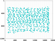
(b)

(c)

Figure 2: The AVDIAR dataset is recorded with a camera-microphone setup. (a) To record the training data, a loud-speaker that emits white noise was used. A visual marker onto the loud-speaker (circled in green) allows to annotate the training data with image locations, each image location corresponds to a loud-speaker direction. (b) The image grid of loud-speaker locations used for the training data. (c) A typical AVDIAR scenario (the camera-microphone setup is circled in green).

In this section we describe the audio-visual datasets that are used to test the proposed method and to compare it with several state-of-the-art methods. We start by describing a novel dataset that was purposively gathered and recorded to encompass a wide number of multiple-speaker scenarios, e.g. speakers facing the camera, moving speakers, speakers looking at each other, etc. This novel dataset is referred to as AVDIAR.

In order to record both training and test data we used the following camera-microphone setup. A color camera is rigidly attached to an acoustic dummy head. The camera is a PointGrey Grasshopper3 unit equipped with a Sony Pregius IMX174 CMOS sensor of size $1.2^{\prime\prime}\times 1^{\prime\prime}$. The camera is equipped with a Kowa 6 mm wide-angle lens and it delivers 1920$\times$1200 color pixels at 25 FPS. This camera-lens setup has a horizontal $\times$ vertical field of view of $97^{\circ}\times 80^{\circ}$.

For the audio recordings we used a binaural Senheiser MKE 2002 dummy head with two microphones plugged into its left and right ears, respectively. The orginal microphone signals are captured at $44100$ Hz, we have downsampled them to $16000$ Hz. The STFT, implemented with a 32 ms Hann window and 16 ms shifts between consecutive windows, is then applied separately to the left and right microphone signals. Therefore, there are 512 samples per frame and the audio frame rate is approximatively 64 FPS. Each audio frame consists of a vector composed $F=256$ Fourier coefficients covering frequencies in the range $0\;\text{Hz}-8\;\text{kHz}$.

The camera and the microphones are connected to a single PC and they are finely synchronized using time stamps delivered by the computer’s internal clock. This audio-visual synchronization allows us to align the visual frames with the audio frames. The time index $t$ corresponds to the visual-frame index. For each $t$ we consider a spectrogram of length $K=25$ frames, or a time slice of 0.4 s, hence there is an overlap between the spectrograms corresponding to consecutive time indexes.

TABLE I: Scenarios available with the AVDIAR dataset.

Recordings	Description
Seq01-1P-S0M1, Seq04-1P-S0M1 , Seq22-1P-S0M1	A single person moving randomly and alternating between speech and silence.
Seq37-2P-S0M0, Seq43-2P-S0M0	Two static participants taking speech turns.
Seq38-2P-S1M0, Seq40-2P-S1M0, Seq44-2P-S2M0	Two static participants speaking almost simultaneously, i.e. there are large speech overlaps.
Seq20-2P-S1M1, Seq21-2P-S2M1	Two participants, wandering in the room and engaged in a conversation, sometime speaking simultaneously.
Seq12-3P-S2M1, Seq27-3P-S2M1	Three participants engaged in an informal conversation. They are moving around and sometimes they speak simultaneously.
Seq13-4P-S1M1, Seq32-4P-S1M1	Three to four participants engaged in a conversation. Sometimes they speak simultaneously and there are many short speech turns.

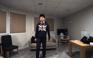
(a)

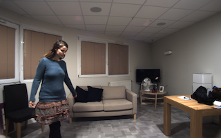
(b)

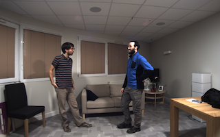
(c)

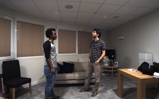
(d)

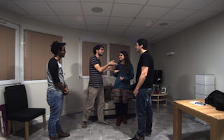
(e)

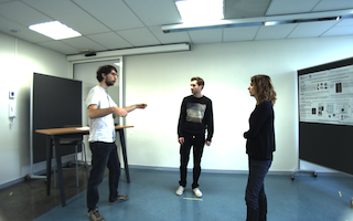
(f)

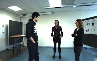
(g)

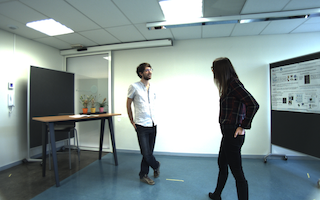
(h)

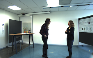
(i)

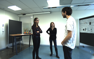
(j)

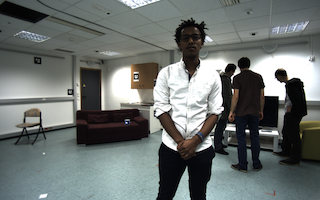
(k)

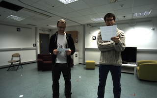
(l)

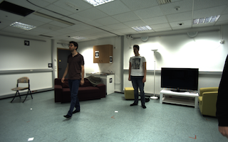
(m)

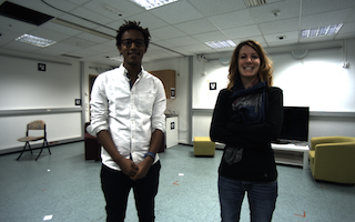
(n)

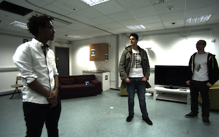
(o)

Figure 3: Examples of scenarios in the AVDIAR dataset. For the sake of varying the acoustic conditions, we used three different rooms to record this dataset.

The training data were recorded by manually moving a loudspeaker in front of the camera-microphone unit e.g. Fig. 2. A visual marker placed at the center of the loudspeaker enables recording of audio signals with their associated pixel positions in the image plane. The loudspeaker is roughly moved in two planes roughly parallel to the image plane, at 1.5 m and 2.5 m, respectively. For each plane we record $800$ positions lying on a uniform 20$\times 40$ grid that covers the entire field of view of the camera, hence there are $M=1600$ training samples. The training data consists of 1 s of white-noise (WN) signals. Using the STFT we therefore obtain two WN spectrograms of size 256$\times$64, corresponding to the left and right microphones, respectively. These two spectrograms are then used to compute binaural feature vectors, i.e. Section V-A (one feature vector for each loud-speaker position) and hence to build a training dataset of audio recordings and their associated image locations $\{\widetilde{\textbf{W}},\widetilde{\mbox{\bf X}}\}=\{(\widetilde{\boldsymbol{W}}_{1},\widetilde{\boldsymbol{X}}_{1}),\dots,(\widetilde{\boldsymbol{W}}_{m},\widetilde{\boldsymbol{X}}_{m}),\dots(\widetilde{\boldsymbol{W}}_{M},\widetilde{\boldsymbol{X}}_{M})\}$, i.e. Section VI.

Similarly we gathered a test dataset that contains several scenarios. Each scenario involves participants that are either static and speak or move and speak, in front of the camera-microphone unit at distance varying between 1.0 m and 3.5 m. In an attempt to record natural human-human interactions, participants were allowed to wonder around the scene and to interrupt each other while speaking. We recorded the following scenario categories, e.g. Fig. 3:

• Static participants facing the camera. This scenario can be used to benchmark diarization methods requiring the detection of frontal faces and of facial and lip movements.

• Static participants facing each other. This scenario can be used to benchmark diarization methods that require static participants not necessarily facing the camera.

• Moving participants. This is a general-purpose scenario that can be used to benchmark diarization as well as audio-visual person tracking.

In addition to the AVDIAR dataset, we used three other datasets, e.g. Fig. 4. They are briefly described as follows:

• The MVAD dataset described in [5]. The visual data were recorded with a Microsoft Kinect sensor at 20 FPS, and the audio signals were recorded with a linear array of omnidirectional microphones sampled at 44100 Hz. The recorded sequences are from 40 s to 60 s long and contain one to three participants that speak in Portuguese. The speech and silence segments are 4 s to 8 s long. Since the diarization method proposed in [5] requires frontal faces, the participants are facing the camera and remain static through all the recordings.

• The AVASM dataset contains both training and test recordings used to test the single and multiple speaker localization method described in [33]. The recording setup is similar to the one described above, namely a binaural acoustic dummy head with two microphones plugged into its ears and a camera placed underneath the head. The images and the audio signals were captured at 25 FPS and 44100 Hz, respectively. The recorded sequences contain up to two participants that face the camera and speak simultaneously. In addition, the dataset has audio-visual alignment data collected in a similar fashion as the AVDIAR dataset.

• The AV16P3 dataset is designed to benchmark audio-visual tracking of several moving speakers without taking diarization into account [42]. The sensor setup used for these recordings is composed of three cameras attached to the room ceiling, and two circular eight-microphone arrays. The recordings include mainly dynamic scenarios, comprising a single, as well as multiple moving speakers. In all the recordings there is a large overlap between the speaker-turns.

These datasets contain a large variety of recorded scenarios, aimed at a wide range of application. e.g. formal and informal interaction in meetings and gatherings, human-computer interaction, etc. Some of the datasets were not purposively recorded to benchmark diarization. Nevertheless they are challenging because they contain a large amount of overlap between speakers, hence they are well suited to test the limits and failures of diarization methods. Unlike recordings of formal meetings, which are composed on long single-speech segments with almost no overlap between the participants, the above datasets contain the following challenging situations e.g. Table I:

• The participants do not always face the cameras, moreover, they turn their heads while they speak or listen;

• The participants, rather then being static, move around and hence the tasks of tracking and diarization must be finely intertwined;

• In informal meetings participants interrupt each other and hence not only that there is no silence between speech segments, but the speech segments overlap each other, and

• Participants take speech turns quite rapidly which results in short-length speech segments, which makes audio-visual temporal alignment quite challenging.

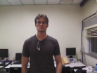
(a)

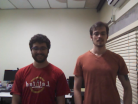
(b)

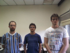
(c)

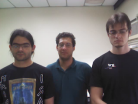
(d)

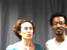
(e)

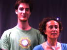
(f)

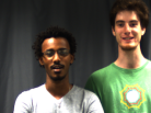
(g)

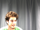
(h)

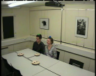
(i)

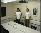
(j)

(k)

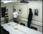
(l)

Figure 4: Example from different datasets. The MVAD dataset (top) contains recordings of one to three persons that always face the camera. The AVASM (middle) was design to benchmark audio-visual sound-source localization with two simultaneously speaking persons or with a moving speaker. The AV16P3 dataset (bottom) contains recordings of simultaneously moving and speaking persons.

VIII Experimental Evaluation

VIII-A Diarization Performance Measure

To effectively benchmark our model with state-of-the art methods, we use the diarization error rate (DER) to quantitatively measure the performance: smaller the DER value, better the performance. DER is defined by the NIST-RT evaluation testbed, and corresponds to the percentage of audio frames that are not correctly assigned to one or more speakers, or to none of them in case of a silent frame. DER consists of the composition of the following measurements:

• False-alarm error, when speech has been incorrectly detected;

• Miss error, when a person is speaking but the method fails to detect the speech activity, and

• Speaker-labeling error, when a person-to-speech association does not correspond to the ground truth.

To compute DER, the md-eval software package of NIST-RT is used, setting the forgiveness collar to a video frame of e.g. 40 ms for 25 FPS videos.

VIII-B Diarization Algorithms and Setup

We compared our method with four methods: [43], [5], [21], and [32]. These methods are briefly explained below:

• Vijayasenan et al. [43] (DiarTK) use audio information only. DiarTK allows the user to incorporate a large number of audio features. In our experiments and comparisons we used the following features: mel-frequency cepstral coefficients (MFCC), frequency-domain linear prediction (FDLP), time difference of arrival (TDOA), and modulation spectrum (MS). Notice that TDOA features can only be used with static sound-sources, hence we did not use TDOA in the case of moving speakers.

• Minotto et al. [5] learn an SVM classifier based on based on labeled audio-visual features. Sound-source localization provides horizontal sound directions which are combined with the output of a mouth tracker.

• Barzelay et al. [21] calculate audio-visual correlations based on extracting onsets from both modalities and on aligning these onsets. The method consists of detecting faces and on tracking face landmarks, such that each landmark yields a trajectory. Onset signals are then extracting from each one of these trajectory as well as from the microphone signal. These onsets are used to compare each visual trajectory with the microphone signal, and the trajectories that best match the microphone signal correspond to the active speaker. We implemented this method based on [21] since there is no publicly available code. Extensive experiments with this method revealed that frontal views of speakers are needed. Therefore, we tested this methods with all the sequences from the MVAD and AVASM datasets and on the sequences from the AVDIAR dataset featuring frontal images of faces.

• Gebru et al. [32] track the active speaker, provided that participants take speech turns with no signal overlap. Therefore, whenever two persons speak simultaneously, this method extracts the dominant speaker.

Additionally, we used the following multiple sound-source localization methods:

• GCC-PHAT which detects the local maxima of the generalized cross-correlation method: we used the implementation from the BSS Locate Toolbox [26].

• TREM which considers a regular grid of source locations and selects the most probable locations based on maximum likelihood: we used the Matlab code provided by the authors, [27].

GCC-PHAT and TREM were used in conjunction with the proposed diarization method using the AVDIAR dataset as well as the MVAD and AV3P16 datasets.

VIII-C Results and Discussion

The results obtained with the MVAD, AVASM, AV16P3 and AVDIAR datasets are summarized in Table II, Table III, Table IV and Table V, respectively.

Overall, it can be noticed that the method of [21] is the least performing method. As explained above this method is based on detecting signal onsets in the two modalities and on finding cross-modal correlations based on onset coincidence. Unfortunately, the visual onsets are unable to properly capture complex speech dynamics. The DiarTK method of [43] is the second least performing method. This is mainly due to the fact that this method is designed to rely on long speech segments with almost no overlap between consecutive segments. Whenever several speech signals overlap, it is very difficult to extract reliable information with MFCC features, since the latter are designed to characterize clean speech. DiarTK is based on clustering MFCC features using a Gaussian mixture model. Consider, for example, MFCC feature vectors of dimension 19, extracted from 20 ms-long audio frames, and a GMM with diagonal covariance matrices. If it is assumed that a minimum of 50 samples are needed to properly estimate the GMM parameters, speech segments of at least 50$\times$19$\times$20 ms, or 19 s, are needed. Therefore it is not surprising that DiarTK performs poorly on all these datasets.

Table II shows that the method of [5] performs much better than DiarTK. This is not surprising, since the speech turns taken by the participants in the MVAD dataset are very brief. Minotto et al. [5] use a combination of visual features extracted form frontal views of faces (lip movements) and audio features (speech-source directions) to train an SVM classifier. The method fails whenever the participants do not face the camera, e.g. sequences Two12, Two13 and Two14, where participants purposely occlude their faces several times throughout the recordings. The method proposed in this paper in combination with TREM achieves the best results on almost all the tested scenarios. This is due to the fact that the audio-visual fusion method is capable of associating very short speech segments with one or several participants. However, the performance of our method, with either TREM or GCC-PHAT, drops down as the number of people increases. This is mainly due to the limited resolution of multiple sound-source localization algorithms (of the order of $10^{\circ}$ horizontally) and thus, it makes it difficult to disambiguate two nearby speaking/silent persons. Notice that tracking the identity of the participants is performed by visual tracking, which is a trivial task for most of these recordings, since participants are mostly static.

Table III shows the results obtained with the AVASM dataset. In these recordings the participants speak simultaneously, with the exception of the Moving-Speaker-01 recording. We do not report results obtained with DiarTK since this method yields non-meaningful performance with this dataset. The proposed method performs reasonable well in the presence of simultaneously speaking persons.

Table IV shows results obtained with the AV16P3 dataset. As with the AVASM dataset we were unable to obtain meaningful results with the DiarTK method. As expected the proposed method has the same performance as [32] in the presence of a single active speaker, e.g. seq11-1p-0100 and seq15-1p-0111. Nevertheless, the performance of [32] rapidly degrades in the presence of two and three persons speaking almost simultaneously. Notice that this dataset was recorded to benchmark audio-visual tracking, not diarization.

TABLE II: DER scores obtained with MVAD dataset (%).

Sequence	DiarTK [43]	[5]	[21]	[32]	Proposed with TREM [27]	Proposed with GCC-PHAT [26]
One7	21.16	8.66	89.90	5.82	0.91	1.06
One8	20.07	7.11	98.10	4.92	1.02	1.81
One9	22.79	9.02	94.60	13.66	0.98	1.58
Two1	23.50	6.81	94.90	16.79	2.87	26.00
Two2	30.22	7.32	90.60	23.49	3.13	13.70
Two3	25.95	7.92	94.50	25.75	8.30	20.88
Two4	25.24	6.91	84.10	20.23	0.16	11.20
Two5	25.96	8.30	90.80	25.02	4.50	29.67
Two6	29.13	6.89	96.70	16.89	6.11	23.57
Two9	30.71	11.95	96.90	15.59	2.42	34.28
Two10	25.32	8.30	95.50	21.04	3.27	15.15
Two11	27.75	6.12	84.60	21.22	6.89	18.05
Two12	45.06	24.60	80.40	39.79	12.00	34.60
Two13	49.23	27.38	64.10	25.11	14.49	48.70
Two14	27.16	28.81	81.10	25.75	6.43	59.10
Three1	27.71	9.10	95.80	47.56	6.17	52.63
Three2	27.71	9.10	89.20	49.15	13.46	49.66
Three3	29.41	5.93	91.50	47.78	13.57	49.09
Three6	36.36	8.92	79.70	40.92	12.89	37.78
Three7	36.24	14.51	86.20	47.35	11.74	40.40
Average	29.33	11.18	89.96	26.69	6.57	28.45

TABLE III: DER scores obtained with AVASM dataset (%).

Sequence	[21]	[32]	Proposed with TREM [27]	Proposed with GCC-PHAT [26]	Proposed
Moving-Speaker-01	95.04	6.26	21.84	17.24	6.26
Two-Speaker-01	70.20	24.11	34.41	44.42	2.96
Two-Speaker-02	80.30	26.98	32.52	47.30	7.33
Two-Speaker-03	74.20	35.26	46.77	47.77	13.78
Average	79.94	23.15	33.89	39.18	7.58

TABLE IV: DER scores obtained with AV16P3 dataset (%).

Sequence	[32]	Proposed with TREM [27]	Proposed with GCC-PHAT [26]
seq11-1p-0100	3.50	3.25	12.18
seq15-1p-0111	3.29	3.29	25.28
seq18-2p-0101	23.54	7.69	9.13
seq24-2p-0111	43.21	17.39	46.50
seq40-3p-1111	26.98	8.51	21.03
Average	20.04	8.02	22.82

TABLE V: DER scores obtained with AVDIAR dataset (%).

Sequence	DiarTK [43]	[21]	[32]	Proposed with TREM [27]	Proposed with GCC-PHAT [26]	Proposed
Seq01-1P-S0M1	43.19	-	14.36	61.15	72.06	3.32
Seq04-1P-S0M1	32.62	-	14.21	71.34	68.84	9.44
Seq22-1P-S0M1	23.53	-	2.76	56.75	67.36	4.93
Seq37-2P-S0M0	12.95	34.70	1.67	41.02	45.90	2.15
Seq43-2P-S0M0	76.10	79.90	23.25	46.81	56.90	6.74
Seq38-2P-S1M0	47.31	59.20	43.01	47.89	47.38	16.07
Seq40-2P-S1M0	48.74	51.80	31.14	42.20	44.62	14.12
Seq20-2P-S1M1	43.58	-	51.78	58.82	59.38	35.46
Seq21-2P-S2M1	32.22	-	27.58	63.03	60.52	20.93
Seq44-2P-S2M0	54.47	-	44.98	55.69	51.0	5.46
Seq12-3P-S2M1	63.67	-	26.55	28.30	61.20	17.32
Seq27-3P-S2M1	46.05	-	20.84	47.40	68.79	18.72
Seq13-4P-S1M1	47.56	-	43.57	28.49	48.23	29.62
Seq32-4P-S1M1	41.51	-	43.26	33.36	71.98	30.20
Average	43.82	56.40	27.78	48.72	58.87	15.32

(a)

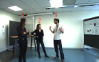
(b)

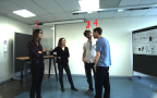
(c)

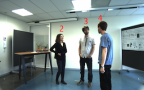
(d)

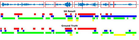
(e)

Figure 5: Results obtained on sequence Seq32-4P-S1M1. Visual tracking results (first row). The raw audio signal delivered by the left microphone and the speech activity region is marked with red rectangles (second row). Speaker diarization result (third row) illustrated with a color diagram: each color corresponds to the speaking activity of a different person. Annotated ground-truth diarization (fourth row).

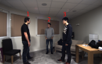
(a)

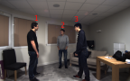
(b)

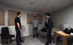
(c)

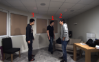
(d)

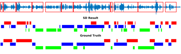
(e)

Figure 6: Results on sequence Seq12-3P-S2M1.

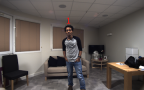
(a)

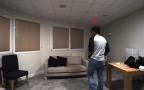
(b)

(c)

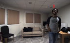
(d)

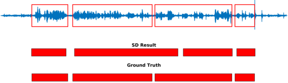
(e)

Figure 7: Results on sequence Seq01-1P-S0M1.

Table V shows the results obtained with the AVDIAR dataset. The content of each scenario is briefly described in Table I. The proposed method outperforms all other methods. It is also interesting to notice that our full method performs better than with either TREM or GCC-PHAT. This is due to the robust semi-supervised audio-visual association method proposed above. Fig. 5, Fig. 6, and Fig. 7 illustrate the audio-visual diarization results obtained by our method with three scenarios.

IX Conclusions

We proposed an audio-visual diarization method well suited for challenging scenarios consisting of participants that either interrupt each other, or speak simultaneously. In both cases, the speech-to-person association problem is a difficult one. We proposed to combine multiple-person visual tracking with multiple speech-source localization in a principled spatiotemporal Bayesian fusion model. Indeed, the diarization process was cast into a latent-variable dynamic graphical model. We described in detail the derivation of the proposed model and we showed that, in the presence of a limited number of speakers (of the order of ten), the diarization formulation is efficiently solved via an exact inference procedure. Then we described a novel multiple speech-source localization method and a weakly supervised audio-visual clustering method.

We also introduced a novel dataset, AVDIAR, that was carefully annotated and that enables to assess the performance of audio-visual (or audio-only) diarization methods using scenarios that were not available with existing datasets, e.g. the participants were allowed to freely move in a room and to turn their heads towards the other participants, rather than always facing the camera. We also benchmarked our method with several other recent methods using publicly available datasets. Unfortunately, we were not able to compare our method with the methods of [2, 3] for two reasons: first, these methods require long speech segments (of the order of 10 s), and second the associated software packages are not publicly available, which would have facilitated the comparison task.

In the future we plan to incorporate richer visual features, such as head pose estimation and head-pose tracking, in order to facilitate the detection of speech turns on the basis of gaze or of people that look at each other over time. We also plan to incorporate richer audio features, such as the possibility to extract speech signals emitted by each participant (sound-source separation) followed by speech recognition, and hence to enable not only diarization but also speech-content understanding. Another extension is to consider distributed sensors, wearable devices, or a combination of both, in order to be able to deal with more complex scenarios involving tens of participants [44, 45].

References

- [1] X. Anguera Miro, S. Bozonnet, N. Evans, C. Fredouille, G. Friedland, and O. Vinyals, “Speaker diarization: A review of recent research,” IEEE Transactions on Audio, Speech, and Language Processing, vol. 20, no. 2, pp. 356–370, 2012.
- [2] G. Garau, A. Dielmann, and H. Bourlard, “Audio-visual synchronisation for speaker diarisation.” in INTERSPEECH, 2010, pp. 2654–2657.
- [3] A. Noulas, G. Englebienne, and B. J. A. Krose, “Multimodal speaker diarization,” IEEE Transactions on Pattern Analysis and Machine Intelligence, vol. 34, no. 1, pp. 79–93, 2012.
- [4] E. El Khoury, C. Sénac, and P. Joly, “Audiovisual diarization of people in video content,” Multimedia tools and applications, vol. 68, no. 3, pp. 747–775, 2014.
- [5] V. P. Minotto, C. R. Jung, and B. Lee, “Multimodal on-line speaker diarization using sensor fusion through SVM,” IEEE Transactions on Multimedia, vol. 17, no. 10, pp. 1694 – 1705, 2015.
- [6] N. Sarafianos, T. Giannakopoulos, and S. Petridis, “Audio-visual speaker diarization using fisher linear semi-discriminant analysis,” Multimedia Tools and Applications, vol. 75, no. 1, pp. 115–130, 2016.
- [7] I. Kapsouras, A. Tefas, N. Nikolaidis, G. Peeters, L. Benaroya, and I. Pitas, “Multimodal speaker clustering in full length movies,” Multimedia Tools and Applications, 2016.
- [8] J. Carletta, S. Ashby, S. Bourban, M. Flynn, M. Guillemot, T. Hain, J. Kadlec, V. Karaiskos, W. Kraaij, M. Kronenthal et al., “The ami meeting corpus: A pre-announcement,” in International Workshop on Machine Learning for Multimodal Interaction. Springer, 2005, pp. 28–39.
- [9] E. Kidron, Y. Y. Schechner, and M. Elad, “Pixels that sound,” in Computer Vision and Pattern Recognition, vol. 1, 2005, pp. 88–95.
- [10] ——, “Cross-modal localization via sparsity,” IEEE Transactions on Signal Processing, vol. 55, no. 4, pp. 1390–1404, 2007.
- [11] M. E. Sargin, Y. Yemez, E. Erzin, and M. A. Tekalp, “Audiovisual synchronization and fusion using canonical correlation analysis,” IEEE Transactions on Multimedia, vol. 9, no. 7, pp. 1396–1403, 2007.
- [12] J. Hershey and J. Movellan, “Audio-vision: Using audio-visual synchrony to locate sounds,” in Advances in Neural Information Processing Systems, 2000, pp. 813–819.
- [13] J. W. Fisher III, T. Darrell, W. T. Freeman, and P. A. Viola, “Learning joint statistical models for audio-visual fusion and segregation,” in NIPS, 2000, pp. 772–778.
- [14] D. Gatica-Perez, G. Lathoud, J.-M. Odobez, and I. McCowan, “Audiovisual probabilistic tracking of multiple speakers in meetings,” IEEE Transactions on Audio, Speech and Language Processing, vol. 15, no. 2, pp. 601–616, 2007.
- [15] S. Naqvi, M. Yu, and J. Chambers, “A multimodal approach to blind source separation of moving sources,” IEEE Journal of Selected Topics in Signal Processing, vol. 4, no. 5, pp. 895 –910, 2010.
- [16] V. Kilic, M. Barnard, W. Wang, and J. Kittler, “Audio assisted robust visual tracking with adaptive particle filtering,” IEEE Transactions on Multimedia, vol. 17, no. 2, pp. 186–200, 2015.
- [17] C. Wooters and M. Huijbregts, “The icsi rt07s speaker diarization system,” in Multimodal Technologies for Perception of Humans. Springer, 2008, pp. 509–519.
- [18] H. Yehia, P. Rubin, and E. Vatikiotis-Bateson, “Quantitative association of vocal-tract and facial behavior,” Speech Communication, vol. 26, no. 1, pp. 23–43, 1998.
- [19] G. Potamianos, C. Neti, G. Gravier, A. Garg, and A. W. Senior, “Recent advances in the automatic recognition of audiovisual speech,” Proceedings of the IEEE, vol. 91, no. 9, pp. 1306–1326, 2003.
- [20] B. Rivet, L. Girin, and C. Jutten, “Mixing audiovisual speech processing and blind source separation for the extraction of speech signals from convolutive mixtures,” IEEE transactions on audio, speech, and language processing, vol. 15, no. 1, pp. 96–108, 2007.
- [21] Z. Barzelay and Y. Y. Schechner, “Onsets coincidence for cross-modal analysis,” IEEE Transactions on Multimedia, vol. 12, no. 2, pp. 108–120, 2010.
- [22] H. J. Nock, G. Iyengar, and C. Neti, “Speaker localisation using audio-visual synchrony: An empirical study,” in International conference on image and video retrieval. Springer, 2003, pp. 488–499.
- [23] M. R. Siracusa and J. W. Fisher, “Dynamic dependency tests for audio-visual speaker association,” in 2007 IEEE International Conference on Acoustics, Speech and Signal Processing-ICASSP’07, vol. 2. IEEE, 2007, pp. II–457.
- [24] A. Noulas and B. J. Krose, “On-line multi-modal speaker diarization,” in Proceedings of the 9th international conference on Multimodal interfaces. ACM, 2007, pp. 350–357.
- [25] M. I. Mandel, R. J. Weiss, and D. P. Ellis, “Model-based expectation-maximization source separation and localization,” IEEE Transactions on Audio, Speech, and Language Processing, vol. 18, no. 2, pp. 382–394, 2010.
- [26] C. Blandin, A. Ozerov, and E. Vincent, “Multi-source tdoa estimation in reverberant audio using angular spectra and clustering,” Signal Processing, vol. 92, no. 8, pp. 1950–1960, 2012.
- [27] Y. Dorfan and S. Gannot, “Tree-based recursive expectation-maximization algorithm for localization of acoustic sources,” IEEE/ACM Transactions on Audio, Speech, and Language Processing, vol. 23, no. 10, pp. 1692–1703, 2015.
- [28] V. Khalidov, F. Forbes, and R. Horaud, “Alignment of Binocular-Binaural Data Using a Moving Audio-Visual Target,” in IEEE Workshop on Multimedia Signal Processing, Pula, Italy, Sep. 2013.
- [29] ——, “Conjugate mixture models for clustering multimodal data,” Neural Computation, vol. 23, no. 2, pp. 517–557, Feb. 2011.
- [30] B. D. Van Veen and K. M. Buckley, “Beamforming: A versatile approach to spatial filtering,” IEEE ASSP Magazine, vol. 5, no. 2, pp. 4–24, 1988.
- [31] I. D. Gebru, S. Ba, G. Evangelidis, and R. Horaud, “Audio-visual speech-turn detection and tracking,” in International Conference on Latent Variable Analysis and Signal Separation, Liberec, Czech Republic, Aug. 2015, pp. 143–151.
- [32] ——, “Tracking the active speaker based on a joint audio-visual observation model,” in Proceedings of the IEEE International Conference on Computer Vision Workshops, Santiago, Chile, 2015, pp. 15–21.
- [33] A. Deleforge, R. Horaud, Y. Y. Schechner, and L. Girin, “Co-localization of audio sources in images using binaural features and locally-linear regression,” IEEE Transactions on Audio, Speech and Language Processing, vol. 23, no. 4, pp. 718–731, 2015.
- [34] I. D. Gebru, X. Alameda-Pineda, F. Forbes, and R. Horaud, “EM algorithms for weighted-data clustering with application to audio-visual scene analysis,” IEEE Transactions on Pattern Analysis and Machine Intelligence, 2016.
- [35] D. Bohus and E. Horvitz, “Decisions about turns in multiparty conversation: from perception to action,” in Proceedings of the 13th international conference on multimodal interfaces. ACM, 2011, pp. 153–160.
- [36] G. Skantze, A. Hjalmarsson, and C. Oertel, “Turn-taking, feedback and joint attention in situated human–robot interaction,” Speech Communication, vol. 65, pp. 50–66, 2014.
- [37] S.-H. Bae and K.-J. Yoon, “Robust online multi-object tracking based on tracklet confidence and online discriminative appearance learning,” in Computer Vision and Pattern Recognition, 2014, pp. 1218–1225.
- [38] L. Bourdev and J. Malik, “Poselets: Body part detectors trained using 3d human pose annotations,” in 2009 IEEE 12th International Conference on Computer Vision. IEEE, 2009, pp. 1365–1372.
- [39] X. Li, L. Girin, R. Horaud, and S. Gannot, “Estimation of relative transfer function in the presence of stationary noise based on segmental power spectral density matrix subtraction,” in IEEE International Conference on Acoustics, Speech and Signal Processing, Brisbane, Australia, Apr. 2015.
- [40] X. Li, R. Horaud, L. Girin, and S. Gannot, “Local relative transfer function for sound source localization,” in European Signal Processing Conference, Nice, France, Aug. 2015.
- [41] X. Li, L. Girin, S. Gannot, and R. Horaud, “Non-stationary noise power spectral density estimation based on regional statistics,” in IEEE International Conference on Acoustics, Speech and Signal Processing (ICASSP). IEEE, 2016, pp. 181–185.
- [42] G. Lathoud, J.-M. Odobez, and D. Gatica-Perez, “Av16. 3: an audio-visual corpus for speaker localization and tracking,” in Machine Learning for Multimodal Interaction. Springer, 2004, pp. 182–195.
- [43] D. Vijayasenan and F. Valente, “Diartk: An open source toolkit for research in multistream speaker diarization and its application to meetings recordings.” in INTERSPEECH, 2012, pp. 2170–2173.
- [44] Y. Yan, E. Ricci, R. Subramanian, O. Lanz, and N. Sebe, “No matter where you are: Flexible graph-guided multi-task learning for multi-view head pose classification under target motion,” in IEEE International Conference on Computer Vision, 2013, pp. 1177–1184.
- [45] X. Alameda-Pineda, Y. Yan, E. Ricci, O. Lanz, and N. Sebe, “Analyzing free-standing conversational groups: a multimodal approach,” in Proceedings of the 23rd ACM International Conference on Multimedia, 2015, pp. 5–14.