Active spanning trees with bending energy on planar maps and SLE-decorated Liouville quantum gravity for $\kappa>8$

Abstract

We introduce a two-parameter family of probability measures on spanning trees of a planar map. One of the parameters controls the activity of the spanning tree and the other is a measure of its bending energy. When the bending parameter is 1, we recover the active spanning tree model, which is closely related to the critical Fortuin–Kasteleyn model. A random planar map decorated by a spanning tree sampled from our model can be encoded by means of a generalized version of Sheffield’s hamburger-cheeseburger bijection. Using this encoding, we prove that for a range of parameter values (including the ones corresponding to maps decorated by an active spanning tree), the infinite-volume limit of spanning-tree-decorated planar maps sampled from our model converges in the peanosphere sense, upon rescaling, to an $\operatorname{SLE}_{\kappa}$-decorated $\gamma$-Liouville quantum cone with $\kappa>8$ and $\gamma=4/\sqrt{\kappa}\in(0,\sqrt{2})$.

1 Introduction

1.1 Overview

We study a family of probability measures on spanning-tree-decorated rooted planar maps, which we define in Section 1.3, using a generalization of the Sheffield hamburger-cheeseburger model [shef-burger]. This family includes as special cases maps decorated by a uniform spanning tree [mullin-maps], planar maps together with a critical Fortuin–Kasteleyn (FK) configuration [shef-burger], and maps decorated by an active spanning tree [kassel-wilson-active]. These models converge in a certain sense (described below) to Liouville quantum gravity (LQG) surfaces decorated by Schramm–Loewner evolution ($\operatorname{SLE}_{\kappa}$) [schramm0], and any value of $\kappa>4$ corresponds to some measure in the family. Although our results are motivated by SLE and LQG, our proofs are entirely self-contained, requiring no knowledge beyond elementary probability theory.

Consider a spanning-tree-decorated rooted planar map $(M,e_{0},T)$, where $M$ is a planar map, $e_{0}$ is an oriented root edge for $M$, and $T$ is a spanning tree of $M$. Let $M^{*}$ be the dual map of $M$ and let $T^{*}$ be the dual spanning tree, which consists of the edges of $M^{*}$ which do not cross edges of $T$. Let $Q$ be the quadrangulation whose vertex set is the union of the vertex sets of $M$ and $M^{*}$, obtained by identifying each vertex of $M^{*}$ with a point in the corresponding face of $M$, then connecting it by an edge (in $Q$) to each vertex of $M$ on the boundary of that face. Each face of $Q$ is bisected by either an edge of $T$ or an edge of $T^{*}$ (but not both). Let $\mathbbm{e}_{0}$ be the oriented edge of $Q$ with the same initial endpoint as $e_{0}$ and which is the first edge in the clockwise direction from $e_{0}$ among all such edges. As explained in, e.g., [shef-burger, § 4.1], there is a path $\lambda$ consisting of edges of (the dual of) $Q$ which snakes between the primal tree $T$ and dual tree $T^{*}$, starts and ends at $\mathbbm{e}_{0}$, and hits each edge of $Q$ exactly once. This path $\lambda$ is called the Peano curve of $(M,e_{0},T)$. See Figure 1 for an illustration.

For Euclidean lattices, Lawler, Schramm, and Werner [lsw-lerw-ust] showed that the uniform spanning tree Peano curve converges to $\operatorname{SLE}_{8}$. For random tree-decorated planar maps with suitable weights coming from the critical Fortuin–Kasteleyn model, Sheffield [shef-burger] proved a convergence result which, when combined with the continuum results of [wedges], implies that the Peano curve converges in a certain sense to a space-filling version of $\operatorname{SLE}_{\kappa}$ with $4<\kappa\leq 8$ on an LQG surface. The measures on tree-decorated planar maps we consider generalize these, and converge in this same sense to $\operatorname{SLE}_{\kappa}$ with $4<\kappa<\infty$.

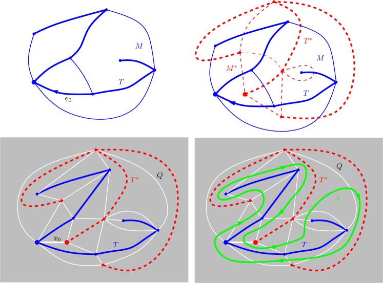
Figure 1: Top left: a rooted map $(M,e_{0})$ (in blue) with a spanning tree $T$ (heavier blue lines). Top right: the dual map $M^{*}$ (dashed red) with the dual spanning tree $T^{*}$ (heavier dashed red lines). Bottom left: the quadrangulation $Q$ (in white) whose vertices are the vertices of $M$ and $M^{*}$. Bottom right: the Peano curve $\lambda$ (in green), exploring clockwise. Formally, $\lambda$ is a cyclic ordering of the edges of $Q$ with the property that successive edges share an endpoint. The triple $(M,e_{0},T)$ can be encoded by means of a two-dimensional simple walk excursion in the first quadrant with $2n$ steps, equivalently a word consisting of elements of the set $\Theta_{0}$ defined below which reduces to the empty word; see Figure 3.

For the measures on tree-decorated planar maps which we consider in this paper, the conjectured scaling limit of the Peano curve $\lambda$ is a whole-plane space-filling $\operatorname{SLE}_{\kappa}$ from $\infty$ to $\infty$ for an appropriate value of $\kappa>4$. In the case when $\kappa\geq 8$, $\operatorname{SLE}_{\kappa}$ is space-filling [schramm-sle], and whole-plane space-filling $\operatorname{SLE}_{\kappa}$ from $\infty$ to $\infty$ is just a whole-plane variant of chordal $\operatorname{SLE}_{\kappa}$ (see [wedges, footnote 9]). It is characterized by the property that for any stopping time $\tau$ for the curve, the conditional law of the part of the curve which has not yet been traced is that of a chordal SLE${}_{\kappa}$ from the tip of the curve to $\infty$. Ordinary $\operatorname{SLE}_{\kappa}$ for $\kappa\in(4,8)$ is not space-filling [schramm-sle]. In this case, whole-plane space-filling $\operatorname{SLE}_{\kappa}$ from $\infty$ to $\infty$ is obtained from a whole-plane variant of ordinary chordal $\operatorname{SLE}_{\kappa}$ by iteratively filling in the “bubbles” disconnected from $\infty$ by the curve. The construction of space-filling $\operatorname{SLE}_{\kappa}$ in this case is explained in [ig4, § 1.2.3 and 4.3]. For $\kappa>4$, whole-plane space-filling $\operatorname{SLE}_{\kappa}$ is the Peano curve of a certain tree of $\operatorname{SLE}_{16/\kappa}$-type curves, namely the set of all flow lines (in the sense of [ig1, ig2, ig3, ig4]) of a whole-plane Gaussian free field (GFF) started from different points but with a common angle.

There are various ways to formulate the convergence of spanning-tree-decorated planar maps toward space-filling $\operatorname{SLE}_{\kappa}$-decorated LQG surfaces. One can embed the map $M$ into $\mathbbm{C}$ (e.g. via circle packing or Riemann uniformization) and conjecture that the Peano curve of $T$ (resp. the measure which assigns mass $1/n$ to each vertex of $M$) converges in the Skorokhod metric (resp. the weak topology) to the space-filling $\operatorname{SLE}_{\kappa}$ (resp. the volume measure associated with the $\gamma$-LQG surface). Alternatively, one can first try to define a metric on an LQG surface (which has so far been accomplished only in the case when $\gamma=\sqrt{8/3}$ [qle, sphere-constructions, tbm-characterization, lqg-tbm1, lqg-tbm2, lqg-tbm3], in which case it is isometric to some variant of the Brownian map [legall-sphere-survey, miermont-survey]), and then try to show that the graph metric on $M$ (suitably rescaled) converges in the Hausdorff metric to an LQG surface. Convergence in the former sense has only recently been shown for “mated-CRT maps” using the Tutte (harmonic or barycentric) embedding [gms-tutte]. It has not yet been proved for any other random planar map model, and convergence in the latter (metric) sense has been established only for uniform planar maps and slight variants thereof (which correspond to $\gamma=\sqrt{8/3}$) [legall-uniqueness, miermont-brownian-map].

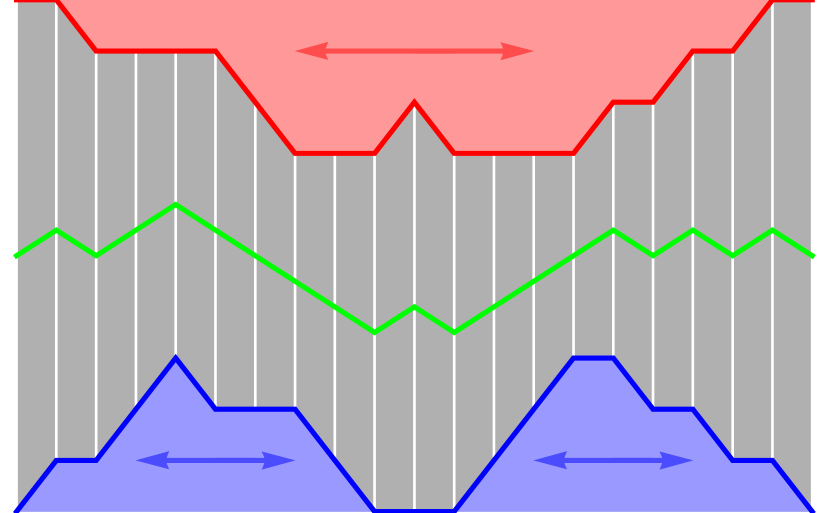
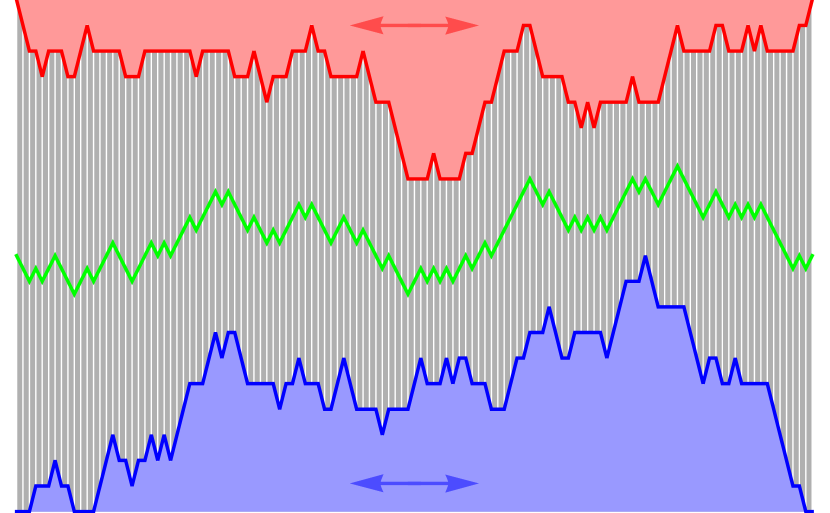
Figure 2: Shown on the top left are the contour functions for the discrete primal tree (blue) and dual tree (red) for the tree-decorated planar map on the bottom left using Sheffield’s hamburger-cheeseburger bijection [shef-burger]. Vertices of the tree and dual tree correspond to blue and red horizontal segments in the contour representation; edges of the tree and dual tree correspond to matching up and down steps. The white boundaries between quadrangles in the quadrangulation correspond to the white vertical segments between the blue and red contour functions; the bold white boundary in the quadrangulation, which marks the starting point of the Peano curve, corresponds to the left and right edges in the contour diagram. The main contribution of the current paper is to establish an infinite volume version of the scaling limit result indicated by the orange horizontal arrow on the top. That is, if one first takes a limit as the size of the map tends to infinity, then the contour functions for the infinite discrete pair of trees converge to a two-dimensional correlated Brownian motion which encode a pair of infinite continuum random trees (CRTs) — this is convergence in the so-called peanosphere sense. The main result of [wedges] implies that these two infinite CRTs glued together as shown (i.e. contracting the vertical white segments in addition to gluing along the horizontal arrows) determine their embedding into an $\operatorname{SLE}$-decorated LQG surface. That is, if one observes the two contour functions on the top right, then one can measurably recover the LQG surface decorated with an $\operatorname{SLE}$ indicated on the bottom right and conversely if one observes the $\operatorname{SLE}$-decorated LQG surface on the bottom right then one can measurably recover the contour functions on the top right. This allows us to interpret our scaling limit result as a convergence result to $\operatorname{SLE}$-decorated LQG.

Here we consider a different notion of convergence, called convergence in the peanosphere sense, which we now describe (see Figure 2). This notion of convergence is based on the work [wedges], which shows how to encode a $\gamma$-quantum cone (a certain type of LQG surface parametrized by $\mathbbm{C}$, obtained by zooming in near a point sampled from the $\gamma$-LQG measure induced by a GFF [wedges, § 4.3]) decorated by an independent whole-plane space-filling $\operatorname{SLE}_{\kappa}$ curve $\eta$ with $\kappa=16/\gamma^{2}$ in terms of a correlated two-dimensional Brownian motion $Z$, with correlation $-\cos(4\pi/\kappa)$. Recall that the contour function of a discrete, rooted plane tree is the function one obtains by tracing along the boundary of the tree starting at the root and proceeding in a clockwise manner and recording the distance to the root from the present vertex. The two coordinates of the Brownian motion $Z$ are the contour functions of the $\operatorname{SLE}_{16/\kappa}$ tree (whose Peano curve is $\eta$) and that of the corresponding dual tree (consisting of GFF flow lines whose angles differ from the angles of the flow lines in the original tree by $\pi$). Here, the distance to the root is measured using $\gamma$-LQG length. On the discrete side, the entire random planar map is determined by the pair of trees. One non-obvious fact established in [wedges] is that the corresponding statement is true in the continuum: the entire $\gamma$-quantum cone and space-filling $\operatorname{SLE}$ turn out to be almost surely determined by the Brownian motion $Z$. We say that the triple $(M,e_{0},T)$ converges in the scaling limit (in the peanosphere sense) to a $\gamma$-quantum cone decorated by an independent whole-plane space-filling $\operatorname{SLE}_{\kappa}$ if the joint law of the contour functions (or some slight variant thereof) of the primal and dual trees $T$ and $T^{*}$ converges in the scaling limit to the joint law of the two coordinates of $Z$.

The present paper is a generalization of [shef-burger], which was the first work to study peanosphere convergence. The paper [shef-burger] considered rooted critical FK planar maps. For $n\in\mathbbm{N}$ and $q\geq 0$, a rooted critical FK planar map with parameter $q$ and size $n$ is a triple $(M,e_{0},S)$ consisting of a planar map $M$ with $n$ edges, a distinguished oriented root edge $e_{0}$ for $M$, and a set $S$ of edges of $M$, sampled with probability proportional to $q^{K(S)/2}$, where $K(S)$ is the number of connected components of $S$ plus the number of complementary connected components of $S$. The conditional law of $S$ given $M$ is that of the self-dual FK model on $M$ [fk-cluster]. An infinite-volume rooted critical FK planar map with parameter $q$ is the infinite-volume limit of rooted critical FK planar maps of size $n$ in the sense of Benjamini–Schramm [benjamini-schramm-topology].

There is a natural (but not bijective) means of obtaining a spanning tree $T$ of $M$ from the FK edge set $S$, which depends on the choice of $e_{0}$; see [bernardi-sandpile, shef-burger]. It is conjectured [shef-burger, wedges] that the triple $(M,e_{0},T)$ converges in the scaling limit to an LQG sphere with parameter $\gamma$ decorated by an independent whole-plane space-filling $\operatorname{SLE}_{\kappa}$ with parameters satisfying

$$\sqrt{q}=-2\cos\mathopen{}\mathclose{{}\left(\frac{4\pi}{\kappa}}\right),\qquad\gamma=\frac{4}{\sqrt{\kappa}}\,.$$ (1.1)

In [shef-burger, Thm. 2.5], this convergence is proven in the peanosphere sense in the case of infinite-volume FK planar maps. This is accomplished by means of a bijection, called the Sheffield hamburger-cheeseburger bijection, between triples $(M,e_{0},S)$ consisting of a rooted planar map of size $n$ and a distinguished edge set $S$; and certain words in an alphabet of five symbols (representing two types of “burgers” and three types of “orders”). This bijection is essentially equivalent for a fixed choice of $M$ to the bijection of [bernardi-sandpile]. The word associated with a triple $(M,e_{0},S)$ gives rise to a walk on $\mathbbm{Z}^{2}$ whose coordinates are (roughly speaking) the contour function of the spanning tree $T$ of $M$ naturally associated with $S$ (under the mapping mentioned in the previous paragraph) and the contour function of the dual spanning tree $T^{*}$ of the dual map $M^{*}$. There is also an infinite-volume version of Sheffield’s bijection which is a.s. well defined for infinite-volume FK planar maps. See [chen-fk] for a detailed exposition of this version of the bijection.

Various strengthenings of Sheffield’s scaling limit result (including an analogous scaling limit result for finite-volume FK planar maps) are proven in [gms-burger-cone, gms-burger-local, gms-burger-finite]. See also [chen-fk, blr-exponents] for additional results on FK planar maps and [gwynne-miller-cle] for a scaling limit result in a stronger topology which is proven using the above peanosphere scaling limit results.

In [kassel-wilson-active], a new family of probability measures on spanning-trees of (deterministic) rooted planar maps, which generalizes the law arising from the self-dual FK model, was introduced. As explained in that paper, the law on trees $T$ of a rooted map $(M,e_{0})$ arising from a self-dual FK model is given by the distribution on all spanning trees of $M$ weighted by $y^{\operatorname{a}(T)}$, where $y=\sqrt{q}+1$ and $\operatorname{a}(T)=\operatorname{a}(T,e_{0})\in\mathbbm{N}$ is the “embedding activity” of $T$ (which depends on the choice of root $e_{0}$; we will remind the reader of the definition later). It also makes sense to consider the probability measure on trees $T$ weighted by $y^{\operatorname{a}(T)}$ for $y\in(0,1)$, so that trees with a lower embedding activity are more likely. The (unifying) discrete model corresponding to any $y\geq 0$ is called a $y$-active spanning tree.

In the context of the current paper, it is natural to look at a joint law on the triple $(M,e_{0},T)$ such that the marginal on $(M,e_{0})$ is the measure which weights a rooted planar map by the partition function of active spanning trees. Indeed, as we explain later, with this choice of law, exploring the tree respects the Markovian structure of the map. We call a random triple sampled from this law a random rooted active-tree-decorated planar map with parameter $y\geq 0$ and size $n\in\mathbbm{N}$. The limiting case $y=0$ corresponds to a spanning tree conditioned to have the minimum possible embedding activity, which is equivalent to a bipolar orientation on $M$ for which the source and sink are adjacent [bernardi-polynomial] (see [kmsw-bipolar] for more on random bipolar-oriented planar maps).

It is conjectured in [kassel-wilson-active] that for $y\in[0,1)$ the scaling limit of a random spanning tree $T$ on large subgraphs of a two-dimensional lattice sampled with probability proportional to $y^{\operatorname{a}(T)}$ is an $\operatorname{SLE}_{\kappa}$ with $\kappa\in(8,12]$ determined by

$$\frac{y-1}{2}=-\cos\mathopen{}\mathclose{{}\left(\frac{4\pi}{\kappa}}\right)\,.$$ (1.2)

It is therefore natural to expect that the scaling limit of a rooted active-tree-decorated planar map is a $\gamma$-LQG surface decorated by an independent space-filling $\operatorname{SLE}_{\kappa}$ with $\kappa\in(8,12]$ as in (1.2) and $\gamma=4/\sqrt{\kappa}$.

We introduce in Section 1.3 a two-parameter family of probability measures on words in an alphabet of 8 symbols which generalizes the hamburger-cheeseburger model of [shef-burger]. Under the bijection of [shef-burger], each of these models corresponds to a probability measure on spanning-tree-decorated planar maps. One parameter in our model corresponds to the parameter $y$ of the active spanning tree, and the other, which we call $z$, controls the extent to which the tree $T$ and its corresponding dual tree $T^{*}$ are “tangled together”. This second parameter can also be interpreted in terms of some form of bending energy of the Peano curve which separates the two trees, in the sense of [bbg-bending, DiFrancesco]; see Remark 1.10. We prove an analogue of [shef-burger, Thm. 2.5] for our model which in particular implies that active-tree-decorated planar maps for $0\leq y<1$ converge in the scaling limit to $\gamma$-quantum cones decorated by $\operatorname{SLE}_{\kappa}$ in the peanosphere sense for $\kappa\in(8,12]$ as in (1.2) and $\gamma=4/\sqrt{\kappa}$. If we also vary $z$, the other parameter of our model, we obtain tree-decorated random planar maps which converge in the peanosphere sense to $4/\sqrt{\kappa}$-quantum cones decorated by space-filling $\operatorname{SLE}_{\kappa}$ for any value of $\kappa>8$.

Remark 1.1.

When $y=0$, an active-tree-decorated planar map is equivalent to a uniformly random bipolar-oriented planar map [bernardi-sandpile]. In [kmsw-bipolar], the authors use a bijective encoding of bipolar-oriented planar maps, which is not equivalent to the one used in this paper, to show that random bipolar-oriented planar maps with certain face degree distributions converge in the peanosphere sense to an $\operatorname{SLE}_{12}$-decorated $\sqrt{4/3}$-LQG surface, both in the finite-volume and infinite-volume cases (see also [ghs-bipolar] for a stronger convergence result). In the special case when $z=1$, our Theorem LABEL:thm-all-S implies convergence of infinite-volume uniform bipolar-oriented planar maps in the peanosphere sense, but with respect to a different encoding of the map than the one used in [kmsw-bipolar]. More precisely, bipolar-oriented maps are encoded in [kmsw-bipolar] by a random walk in $\mathbbm{Z}^{2}$ with a certain step distribution. The encoding of bipolar-oriented maps by the generalized hamburger-cheeseburger bijection corresponds to a random walk in $\mathbbm{Z}^{2}\times\{0,1\}$ with a certain step distribution. Both of these walks converge in law to a correlated Brownian motion (ignoring the extra bit in the hamburger-cheeseburger bijection), and the correlations are the same, so we say that they both converge in the peanosphere sense.

1.2 Basic notation

We write $\mathbbm{N}$ for the set of positive integers.

For $a<b\in\mathbbm{R}$, we define the discrete intervals $[a,b]_{\mathbbm{Z}}\colonequals[a,b]\cap\mathbbm{Z}$ and $(a,b)_{\mathbbm{Z}}\colonequals(a,b)\cap\mathbbm{Z}$.

If $a$ and $b$ are two quantities, we write $a\preceq b$ (resp. $a\succeq b$) if there is a constant $C$ (independent of the parameters of interest) such that $a\leq Cb$ (resp. $a\geq Cb$). We write $a\asymp b$ if $a\preceq b$ and $a\succeq b$.

1.3 Generalized burger model

We now describe the family of words of interest to us in this paper. These are (finite or infinite) words which we read from left to right and which consist of letters representing burgers and orders which are matched to one another following certain rules. Several basic properties of this model are proved in Appendix LABEL:sec-prelim. Let

$$\Theta_{0}\colonequals\mathopen{}\mathclose{{}\left\{{\mathsf{h}},{\mathsf{c}},{\mathsf{H}},{\mathsf{C}}}\right\},$$ (1.3)

and let $\mathcal{W}(\Theta_{0})$ be the set of all finite words consisting of elements of $\Theta_{0}$. The alphabet $\Theta_{0}$ generates a semigroup whose elements are words in $\mathcal{W}(\Theta_{0})$ modulo the relations

$$\begin{split}&{\mathsf{c}}{\mathsf{C}}={\mathsf{h}}{\mathsf{H}}=\emptyset\quad\quad\quad\text{(order fulfillment)}\\ &{\mathsf{c}}{\mathsf{H}}={\mathsf{H}}{\mathsf{c}},\quad{\mathsf{h}}{\mathsf{C}}={\mathsf{C}}{\mathsf{h}}.\end{split}$$ (1.4)

Following Sheffield [shef-burger], we think of ${\mathsf{h}},{\mathsf{c}},{\mathsf{H}},{\mathsf{C}}$ as representing a hamburger, a cheeseburger, a hamburger order, and a cheeseburger order, respectively. A hamburger order is fulfilled by the freshest available hamburger (i.e., the rightmost hamburger which has not already fulfilled an order) and similarly for cheeseburger orders. We say that an order and a burger which cancel out via the first relation of (1.4) have been matched, and that the order has consumed the burger. See Fig. 3 (a) for a diagram representing matchings in an example.

We enlarge the alphabet by defining

$$\Theta\colonequals\Theta_{0}\cup\mathopen{}\mathclose{{}\left\{{\mathsf{d}},{\mathsf{e}},{\mathsf{F}},{\mathsf{S}}}\right\},$$ (1.5)

and let $\mathcal{W}(\Theta)$ be the set of all finite words consisting of elements of $\Theta$. The alphabet $\Theta$ generates a semigroup whose elements are finite words consisting of elements of $\Theta$ modulo the relations (1.4) and the additional relations

$${\mathsf{h}}{\mathsf{F}} ={\mathsf{h}}{\mathsf{H}}=\emptyset \quad{\mathsf{c}}{\mathsf{F}} ={\mathsf{c}}{\mathsf{C}}=\emptyset$$ (1.6)

$${\mathsf{h}}{\mathsf{S}} ={\mathsf{h}}{\mathsf{C}} {\mathsf{c}}{\mathsf{S}} ={\mathsf{c}}{\mathsf{H}}$$

$${\mathsf{h}}{\mathsf{d}} ={\mathsf{h}}{\mathsf{h}} {\mathsf{c}}{\mathsf{d}} ={\mathsf{c}}{\mathsf{c}}$$

$${\mathsf{h}}{\mathsf{e}} ={\mathsf{h}}{\mathsf{c}} {\mathsf{c}}{\mathsf{e}} ={\mathsf{c}}{\mathsf{h}}.$$

In the language of burgers, the symbol ${\mathsf{F}}$ represents a “flexible order” which requests the freshest available burger. The symbol ${\mathsf{S}}$ represents a “stale order” which requests the freshest available burger of the type opposite the freshest available burger. The symbol ${\mathsf{d}}$ represents a “duplicate burger” which acts like a burger of the same type as the freshest available burger. The symbol ${\mathsf{e}}$ represents an “opposite burger” which acts like a burger of the type opposite the freshest available burger. The model of [shef-burger] includes the flexible order ${\mathsf{F}}$ but no other elements of $\Theta\setminus\Theta_{0}$.

If a symbol in $\mathopen{}\mathclose{{}\left\{{\mathsf{d}},{\mathsf{e}},{\mathsf{F}},{\mathsf{S}}}\right\}$ has been replaced by a symbol in $\Theta_{0}$ via one of the relations in (1.6), we say that this symbol is identified by the earlier symbol in the relation; and identified as the symbol in $\Theta_{0}$ with which it has been replaced.

Given a word $x=x_{1}\cdots x_{n}\in\mathcal{W}(\Theta)$, we write $|x|=n$ for the number of symbols in $x$.

Definition 1.2.

A word in $\mathcal{W}(\Theta)$ is called reduced if all of its orders, ${\mathsf{d}}$’s, and ${\mathsf{e}}$’s lie to the left of all of its ${\mathsf{h}}$’s and ${\mathsf{c}}$’s. In Lemma LABEL:prop-reduction we show that for any finite word $x$, there is a unique reduced word which can be obtained from $x$ by applying the relations (1.4) and (1.6), which we call the reduction of $x$, and denote by $\hyperlink{def-reduce}{\mathcal{R}}(x)$.

An important property of the reduction operation (proved in Lemma LABEL:prop-associative) is

$$\hyperlink{def-reduce}{\mathcal{R}}(xy)=\hyperlink{def-reduce}{\mathcal{R}}(\hyperlink{def-reduce}{\mathcal{R}}(x)\hyperlink{def-reduce}{\mathcal{R}}(y)).$$

Note that for any $x\in\mathcal{W}(\Theta)$, we have $|\hyperlink{def-reduce}{\mathcal{R}}(x)|\leq|x|$.

Definition 1.3.

We write $x^{\prime}=\hyperlink{def-identification}{\mathcal{I}}(x)$ (the identification of $x$) for the word with $|x^{\prime}|=|x|$ obtained from $x$ as follows. For each $i\in\{1,\ldots,|x|\}$, if $x_{i}\in\Theta_{0}$, we set $x_{i}^{\prime}=x_{i}$. If $x_{i}\in\{{\mathsf{F}},{\mathsf{S}}\}$ and $x_{i}$ is replaced by a hamburger order (resp. cheeseburger order) via (1.6) when we pass to the reduced word $\hyperlink{def-reduce}{\mathcal{R}}(x)$, we set $x_{i}^{\prime}={\mathsf{H}}$ (resp. $x_{i}^{\prime}={\mathsf{C}}$). If $x_{i}\in\{{\mathsf{d}},{\mathsf{e}}\}$ and $x_{i}$ is replaced with a hamburger (resp. cheeseburger) via (1.6) when we pass to the reduced word, we set $x_{i}^{\prime}={\mathsf{h}}$ (resp. $x_{i}^{\prime}={\mathsf{c}}$). Otherwise, we set $x_{i}^{\prime}=x_{i}$. We say that a symbol $x_{i}$ is identified in the word $x$ if $x_{i}^{\prime}$ is an element of $\Theta_{0}$, and unidentified in the word $x$ otherwise.

For example,

$$\hyperlink{def-reduce}{\mathcal{R}}\mathopen{}\mathclose{{}\left({\mathsf{c}}{\mathsf{F}}{\mathsf{d}}{\mathsf{h}}{\mathsf{S}}}\right) ={\mathsf{d}}{\mathsf{C}}{\mathsf{h}}$$

$$\hyperlink{def-identification}{\mathcal{I}}\mathopen{}\mathclose{{}\left({\mathsf{c}}{\mathsf{F}}{\mathsf{d}}{\mathsf{h}}{\mathsf{S}}}\right) ={\mathsf{c}}{\mathsf{C}}{\mathsf{d}}{\mathsf{h}}{\mathsf{C}}.$$

Note that $\hyperlink{def-reduce}{\mathcal{R}}(\hyperlink{def-identification}{\mathcal{I}}(x))=\hyperlink{def-reduce}{\mathcal{R}}(x)$. Note also that any symbol $x_{i}$ which has a match when we pass to $\hyperlink{def-reduce}{\mathcal{R}}(x)$ is necessarily identified, but identified symbols are not necessarily matched. Indeed, symbols in $\Theta_{0}$ are always identified, and there may be ${\mathsf{S}}$, ${\mathsf{d}}$, and/or ${\mathsf{e}}$ symbols in $x$ which are identified, but do not have a match.

Definition 1.4.

For $\theta\in\Theta$ and a finite word $x$ consisting of elements of $\Theta$, we write

$$\hyperlink{def-theta-count}{\mathcal{N}\!}_{\theta}(x) \colonequals\text{number of $\theta$-symbols in $x$}$$

$$\hyperlink{def-theta-count}{\mathcal{N}\!}_{\theta_{1}|\cdots|\theta_{k}}(x) \colonequals\hyperlink{def-theta-count}{\mathcal{N}\!}_{\theta_{1}}(x)+\cdots+\hyperlink{def-theta-count}{\mathcal{N}\!}_{\theta_{k}}(x)$$

We also define

$$\hyperlink{def-theta-count}{\mathcal{B}}(x) \colonequals\hyperlink{def-theta-count}{\mathcal{N}\!}_{{\mathsf{h}}|{\mathsf{c}}|{\mathsf{d}}|{\mathsf{e}}}(x)=\text{number of burgers in $x$}$$

$$\hyperlink{def-theta-count}{\mathcal{O}}(x) \colonequals\hyperlink{def-theta-count}{\mathcal{N}\!}_{{\mathsf{H}}|{\mathsf{C}}|{\mathsf{F}}|{\mathsf{S}}}(x)=\text{number of orders in $x$}$$

$$\hyperlink{def-theta-count}{\mathcal{C}}(x) \colonequals\hyperlink{def-theta-count}{\mathcal{B}}(x)-\hyperlink{def-theta-count}{\mathcal{O}}(x)$$

and

$$\hyperlink{def-theta-count}{d}(x) \colonequals\hyperlink{def-theta-count}{\mathcal{N}\!}_{{\mathsf{h}}}(x)-\hyperlink{def-theta-count}{\mathcal{N}\!}_{{\mathsf{H}}}(x)$$

$$\hyperlink{def-theta-count}{d^{*}}(x) \colonequals\hyperlink{def-theta-count}{\mathcal{N}\!}_{{\mathsf{c}}}(x)-\hyperlink{def-theta-count}{\mathcal{N}\!}_{{\mathsf{C}}}(x)$$

$$\hyperlink{def-theta-count}{\vec{d}}(x) \colonequals\mathopen{}\mathclose{{}\left(\hyperlink{def-theta-count}{d}(x),\,\hyperlink{def-theta-count}{d^{*}}(x)}\right)$$

$$\hyperlink{def-theta-count}{\mathcal{D}}(x) \colonequals\hyperlink{def-theta-count}{d}(x)-\hyperlink{def-theta-count}{d^{*}}(x)\,.$$

The reason for the notation d and d∗ is that these quantities represent distances to the root edge in the primal and dual trees, respectively, in the construction of [shef-burger, § 4.1] (see the discussion just below). Note that these quantities are still defined even if $x$ has some symbols in $\mathopen{}\mathclose{{}\left\{{\mathsf{d}},{\mathsf{e}},{\mathsf{F}},{\mathsf{S}}}\right\}$.

Fig. 3 (b) shows a random-walk representation of →d computed on increasing prefixes of a finite (identified) word. This process will later be our main object of study.

If $x$ is a finite word consisting of elements of $\Theta$ with $\hyperlink{def-reduce}{\mathcal{R}}(x)=\emptyset$, then the bijection described in [shef-burger, § 4.1] applied to $\hyperlink{def-identification}{\mathcal{I}}(x)$ uniquely determines a rooted spanning-tree-decorated map $(M,e_{0},T)$ associated with $x$.

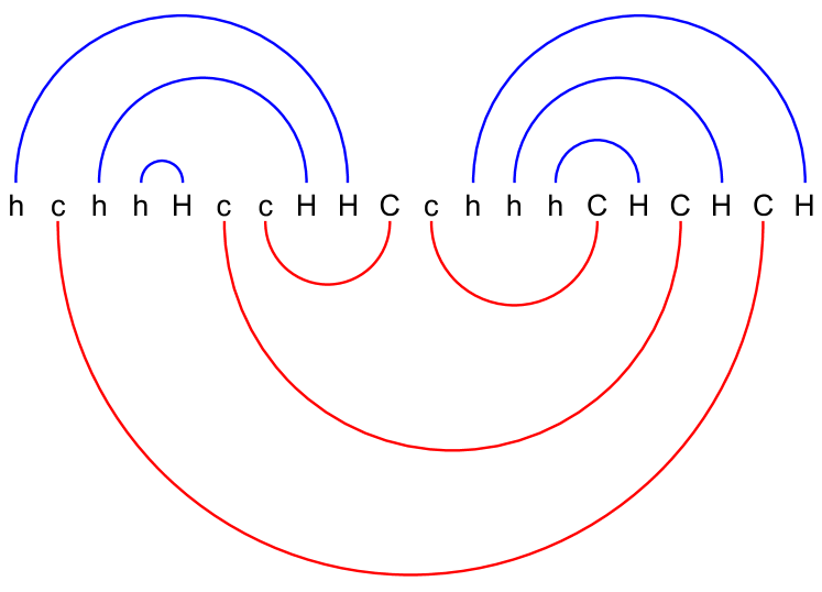
(a) The word associated to the decorated map of Fig. 1. The chords represent the matchings between orders and burgers that fulfill them.

(b) The trace of the walk $(\hyperlink{def-theta-count}{\vec{d}}_{i})_{0\leq i\leq|x|}$ corresponding to the →d vector of increasing prefixes of the word $x={\mathsf{h}}{\mathsf{c}}{\mathsf{h}}{\mathsf{h}}{\mathsf{H}}{\mathsf{c}}{\mathsf{c}}{\mathsf{H}}{\mathsf{H}}{\mathsf{C}}{\mathsf{c}}{\mathsf{h}}{\mathsf{h}}{\mathsf{h}}{\mathsf{C}}{\mathsf{H}}{\mathsf{C}}{\mathsf{H}}{\mathsf{C}}{\mathsf{H}}$. The walk gives the number of available hamburgers and cheeseburgers as a function of time.

Figure 3:

We now describe the probability measure on words which gives rise to the law on spanning-tree-decorated planar maps which we are interested in. Let

$$\mathcal{P}\colonequals\mathopen{}\mathclose{{}\left\{(p_{\mathsf{F}},p_{\mathsf{S}},p_{\mathsf{d}},p_{\mathsf{e}})\in[0,1]^{4}\,:\,p_{\mathsf{F}}+p_{\mathsf{S}}\leq 1\quad\operatorname{and}\quad p_{\mathsf{d}}+p_{\mathsf{e}}<1}\right\}.$$

For a vector $\vec{p}=(p_{\mathsf{F}},p_{\mathsf{S}},p_{\mathsf{d}},p_{\mathsf{e}})\in\mathcal{P}$, we define a probability measure $\mathbbm{P}=\mathbbm{P}_{\vec{p}}$ on $\Theta$ by

$$\mathbbm{P}\!\mathopen{}\mathclose{{}\left({\mathsf{F}}}\right) =\frac{p_{\mathsf{F}}}{2}, \mathbbm{P}\!\mathopen{}\mathclose{{}\left({\mathsf{S}}}\right) =\frac{p_{\mathsf{S}}}{2}, \mathbbm{P}\!\mathopen{}\mathclose{{}\left({\mathsf{H}}}\right)=\mathbbm{P}\!\mathopen{}\mathclose{{}\left({\mathsf{C}}}\right) =\frac{1-p_{\mathsf{F}}-p_{\mathsf{S}}}{4}$$ (1.7)

$$\mathbbm{P}\!\mathopen{}\mathclose{{}\left({\mathsf{d}}}\right) =\frac{p_{\mathsf{d}}}{2}, \mathbbm{P}\!\mathopen{}\mathclose{{}\left({\mathsf{e}}}\right) =\frac{p_{\mathsf{e}}}{2}, \mathbbm{P}\!\mathopen{}\mathclose{{}\left({\mathsf{h}}}\right)=\mathbbm{P}\!\mathopen{}\mathclose{{}\left({\mathsf{c}}}\right) =\frac{1-p_{\mathsf{d}}-p_{\mathsf{e}}}{4}.$$

Let $X=\cdots X_{-1}X_{0}X_{1}\cdots$ be a bi-infinite word whose symbols are i.i.d. samples from the probability measure (1.7). The identification procedure extends naturally to bi-infinite words, and we show in Appendix LABEL:sec-prelim that a.s. the bi-infinite identified word $X^{\prime}=\hyperlink{def-identification}{\mathcal{I}}(X)$ exists and contains only elements of $\Theta_{0}$. Furthermore, a.s. each order in $X$ consumes a burger and each burger in $X$ is consumed by an order. That is, each symbol $X_{i}$ in $X$ has a match $X_{\phi(i)}$ which cancels it out, so that in effect the reduced bi-infinite word $\hyperlink{def-reduce}{\mathcal{R}}(X)$ is a.s. empty.

Definition 1.5.

We write $X^{\prime}=\cdots X_{-1}^{\prime}X_{0}^{\prime}X_{1}^{\prime}\cdots$ for the identification of the bi-infinite word $X$.

Definition 1.6.

For $i\in\mathbbm{Z}$, we write $\phi(i)\in\mathbbm{Z}$ for the index of the symbol matched to $X_{i}$ in the word $X$. (From the above property, a.s. $\phi$ is an involution of $\mathbbm{Z}$.)

For $a<b\in\mathbbm{R}$, we write

$$X(a,b)\colonequals\hyperlink{def-reduce}{\mathcal{R}}(X_{\lfloor a\rfloor}\cdots X_{\lfloor b\rfloor})\quad\operatorname{and}\quad X^{\prime}(a,b)\colonequals\hyperlink{def-reduce}{\mathcal{R}}(X_{\lfloor a\rfloor}^{\prime}\cdots X_{\lfloor b\rfloor}^{\prime}).$$ (1.8)

The aforementioned results of Appendix LABEL:sec-prelim allow us to use the infinite-volume version of Sheffield’s bijection [shef-burger] (which is described in full detail in [chen-fk]) to construct an infinite-volume rooted spanning-tree-decorated planar map $(M^{\infty},e_{0},T^{\infty})$ from the identified word $X^{\prime}$ of Definition 1.5.

The set $\mathcal{P}$ describes a four-parameter family of probability measures on $\Theta$, and hence a four-parameter family of probability measures on triples $(M^{\infty},e_{0},T^{\infty})$. However, as we will see in Corollary 1.13 below, the law of $X^{\prime}$ (and hence also the law of $(M^{\infty},e_{0},T^{\infty})$) depends only on the two parameters $p_{\mathsf{F}}-p_{\mathsf{S}}$ and $p_{\mathsf{d}}-p_{\mathsf{e}}$ (equivalently the parameters $y$ and $z$ defined in (1.11)).

Remark 1.7.

The model described above includes three special symbols which are natural generalizations of the special order ${\mathsf{F}}$ included in [shef-burger]: the order ${\mathsf{S}}$ has the opposite behavior as the order ${\mathsf{F}}$, and the burgers ${\mathsf{d}}$ and ${\mathsf{e}}$ behave in the same way as ${\mathsf{S}}$ and ${\mathsf{F}}$ but with burgers in place of orders. As we will see in Section 1.4, each of these symbols has a natural topological interpretation in terms of the spanning-tree-decorated rooted planar maps encoded by words consisting of elements of $\Theta$.

Remark 1.8.

As we will see, the words we consider in this paper can behave in very different ways from the words considered in [shef-burger], which do not include the symbols ${\mathsf{S}},{\mathsf{d}},$ or ${\mathsf{e}}$. For example, in the setting of Section LABEL:sec-variable-SD, where we allow ${\mathsf{S}}$’s and ${\mathsf{d}}$’s but not ${\mathsf{F}}$’s or ${\mathsf{e}}$’s, the net hamburger/cheeseburger counts $\hyperlink{def-theta-count}{d}(X(1,n))$ and $\hyperlink{def-theta-count}{d^{*}}(X(1,n))$ in a reduced word tend to be negatively correlated (Theorem LABEL:thm-variable-SD) and the reduced word $X(1,n)$ tends to have more symbols than the corresponding reduced word in the case when $p_{\mathsf{F}}=p_{\mathsf{S}}=p_{\mathsf{d}}=p_{\mathsf{e}}=0$ (Lemma LABEL:prop-mean-mono). The opposite is true in the setting of [shef-burger]. As another example, in the setting of Section LABEL:sec-variable-SD we expect, but do not prove, that the infinite reduced word $X(1,\infty)$ a.s. contains only finitely many unidentified ${\mathsf{S}}$’s and ${\mathsf{d}}$’s, whereas $X(1,\infty)$ a.s. contains infinitely many unidentified ${\mathsf{F}}$’s in the setting of [shef-burger] (Remark LABEL:remark-I-infinite).

1.4 Active spanning trees with bending energy

Let $(M,e_{0})$ be a (deterministic) planar map with $n$ edges with oriented root edge $e_{0}$. Let $M^{*}$ be the dual map of $M$ and let $(Q,\mathbbm{e}_{0})$ be the associated rooted quadrangulation (as described at the beginning of the introduction). In this subsection we introduce a probability measure on spanning trees of $M$ which is encoded by the model of Section 1.3.

There is a bijection between spanning trees on $M$ and noncrossing Eulerian cycles on the medial graph of $M$, which is the planar dual graph of $Q$. (An Eulerian cycle is a cycle which traverses each edge exactly once, vertices may be repeated.) To describe this bijection, let $\lambda$ be a noncrossing Eulerian cycle on the dual of $Q$ starting and ending at $\mathbbm{e}_{0}$. By identifying an edge of $Q^{*}$ with the edge of $Q$ which crosses it, we view $\lambda$ as a function from $[1,2n]_{\mathbbm{Z}}$ to the edge set of $Q$. Each quadrilateral of $Q$ is bisected by one edge of $M$ and one edge of $M^{*}$, and $\lambda$ crosses each such quadrilateral exactly twice (one such quadrilateral is shown in gray in Figure 4). Hence $\lambda$ crosses each edge of $M$ and each edge of $M^{*}$ either 0 or 2 times. The set $T$ of edges of $M$ which are not crossed by $\lambda$ is a spanning tree of $M$ whose discrete Peano curve is $\lambda$ and the set $T^{*}$ of edges of $M^{*}$ not crossed by $\lambda$ is the corresponding dual spanning tree of $M^{*}$. Each quadrilateral of $Q$ is bisected by an edge of either $T$ or $T^{*}$ (but not both). This establishes a one-to-one correspondence between noncrossing Eulerian cycles on the dual of $Q$ starting and ending at $\mathbbm{e}_{0}$ and spanning trees of $M$.

Now fix a noncrossing Eulerian cycle $\lambda$ as above. For $i\in[1,2n]_{\mathbbm{Z}}$ we let $\overline{e}_{i}$ be the edge of $T\cup T^{*}$ which bisects the last quadrilateral of $Q$ crossed by $\lambda$ exactly once at or before time $i$, if such a quadrilateral exists. Let $e$ be an edge of $T\cup T^{*}$, and let $j,k\in[1,2n]_{\mathbbm{Z}}$ be the first and second times respectively that $\lambda$ crosses the quadrilateral of $Q$ bisected by $e$. Observe that if $e$ and $\overline{e}_{k-1}$ both belong to $M$ or both belong to $M^{*}$, then in fact $e=\overline{e}_{k-1}$. In this case, we say that $e$ is of active type; this definition coincides with “embedding activity”, as illustrated in Figure 4. If $\overline{e}_{j-1}$ exists and $e$ and $\overline{e}_{j-1}$ either both belong to $M$ or both belong to $M^{*}$, then we say that $e$ is of duplicate type; duplicate edges are illustrated in Figure 5, and Remark 1.10 below discusses their relevance. Figure 6 shows the active and duplicate edges from Figure 1. An edge can be of both active and duplicate type, or of neither active nor duplicate type.

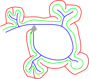
$\rightarrow$

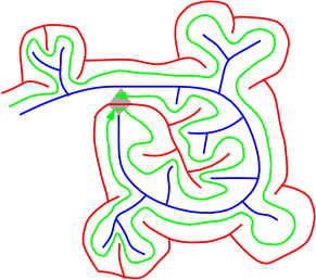
Figure 4: The Peano exploration process with the Peano path $\lambda$ in green, primal tree $T$ in blue, and dual tree $T^{*}$ in red. When the gray quadrilateral is first encountered (left panel), the dual edge $e$ is forced to be present (otherwise there would be a primal cycle). This means that $e$ is “embedding active”, in the sense of [bernardi-sandpile] (see also [courtiel-activity]). The Peano curve then explores the map in the region enclosed by the blue near-cycle and exits through the same (gray) quadrilateral (right panel). Just before the second time the gray quadrilateral is encountered, the most recent quadrilateral encountered exactly once is the gray quadrilateral, so $\bar{e}_{k-1}=e$, so $e$ is of active type as defined above. This characterization of the embedding activity was explained in [shef-burger].

Following [bernardi-sandpile, shef-burger], a noncrossing Eulerian cycle $\lambda$ based at $\mathbbm{e}_{0}$ can be encoded by means of a word $x$ of length $2n$ consisting of elements of $\Theta_{0}$ with reduced word $\hyperlink{def-reduce}{\mathcal{R}}(x)=\emptyset$. The symbol ${\mathsf{h}}$ (resp. ${\mathsf{H}}$) corresponds to the first (resp. second) time that $\lambda$ crosses an edge of $M$, and the symbol ${\mathsf{c}}$ (resp. ${\mathsf{C}}$) corresponds to the first (resp. second) time that $\lambda$ crosses an edge of $M^{*}$. The two times that $\lambda$ crosses a given quadrilateral of $Q$ correspond to a burger and the order which consumes it. With $\overline{e}_{i}$ as above, the burger corresponding to the quadrilateral bisected by $\overline{e}_{i}$ is the same as the rightmost burger in the reduced word $\hyperlink{def-reduce}{\mathcal{R}}(x_{1}\cdots x_{i})$; the edge $\overline{e}_{i}$ is undefined if and only if this reduced word is empty. Therefore edges of active type correspond to orders which consume the most recently added burger that has not yet been consumed, and edges of duplicate type correspond to burgers which are the same type as the the most recently added burger that has not yet been consumed.

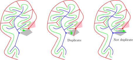
Figure 5: Left: the two trees $T$ and $T^{*}$ and the Peano curve $\lambda$ (in green) run up until step $i-1$. The pink quadrilateral is the most recent one which has been crossed exactly once by $\lambda$ by time $i-1$ and $\overline{e}_{i-1}$ is the red edge which bisects this quadrilateral. The vertices $v_{i-1}^{0}$ and $v_{i-1}^{1}$ discussed in Remark 1.10 are shown in red and blue, respectively. At step $i$, $\lambda$ will either bend away from the red vertex (middle) or toward the red vertex (right). In the former case the edge which bisects the grey quadrilateral belongs to the same tree as $\overline{e}_{i-1}$, so the edge $\lambda(i)$ is of duplicate type.

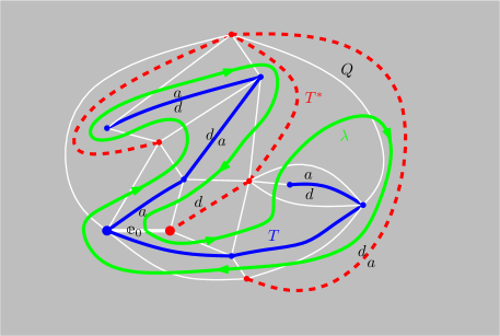
Figure 6: The quadrangulation $Q$, the trees $T$ and $T^{*}$, and the Peano curve $\lambda$ constructed from the triple $(M,e_{0},T)$ of Figure 1 with active (resp. duplicate) edges of $T\cup T^{*}$ indicated with an $a$ (resp. a $d$). Edges can be both active and duplicate. The root edge $\mathbbm{e}_{0}$ is indicated by a thicker white line. If we allow symbols in $\Theta$ (rather than just $\Theta_{0}$), the triple $(M,e_{0},T)$ can be encoded by many different words of length $2n$; more precisely, it can be encoded by any word whose identification is the word shown in Figure 3. The word corresponding to $(M,e_{0},T)$ with the smallest possible number of elements of $\Theta_{0}$ is ${\mathsf{h}}{\mathsf{e}}{\mathsf{e}}{\mathsf{d}}{\mathsf{F}}{\mathsf{e}}{\mathsf{d}}{\mathsf{S}}{\mathsf{S}}{\mathsf{F}}{\mathsf{c}}{\mathsf{e}}{\mathsf{d}}{\mathsf{d}}{\mathsf{S}}{\mathsf{F}}{\mathsf{S}}{\mathsf{F}}{\mathsf{S}}{\mathsf{F}}$. In this word, ${\mathsf{F}}$ (resp. ${\mathsf{S}}$) symbols correspond to the second time $\lambda$ crosses a quadrilateral of $Q$ bisected by an active (resp. inactive) edge and ${\mathsf{d}}$ (resp. ${\mathsf{e}}$) symbols correspond to the first time $\lambda$ crosses a quadrilateral of $Q$ bisected by a duplicate (resp. non-duplicate) edge. The ${\mathsf{h}}$ and ${\mathsf{c}}$ symbols correspond to times $i$ for which the edge $\overline{e}_{i}$ is not defined.

For a spanning tree $T$ of $M$ rooted at $e_{0}$, we let $\operatorname{a}(T)$ be the number of active edges and $\operatorname{d}(T)$ the number of duplicate edges of its Peano curve $\lambda$. These quantities depend on the choice of $e_{0}$. We define the partition function

$$\mathcal{Z}(M,e_{0},y,z)=\sum_{\text{spanning tree}\,T}y^{\operatorname{a}(T)}z^{\operatorname{d}(T)}\,,$$ (1.9)

which gives rise, when $y,z\geq 0$, to a probability measure

$$\mathbbm{P}[T]=\frac{y^{\operatorname{a}(T)}z^{\operatorname{d}(T)}}{\mathcal{Z}(M,e_{0},y,z)}\,,$$ (1.10)

on the set of spanning trees $T$ of $M$. This distribution on spanning trees satisfies a domain Markov property: for $i\in[1,2n]_{\mathbbm{Z}}$, the conditional law of $\lambda|_{[i+1,2n]_{\mathbbm{Z}}}$ given $\lambda|_{[1,i]_{\mathbbm{Z}}}$ depends only on the set of quadrilaterals and half-quadrilaterals not yet visited by $\lambda$ together with the starting and ending points of the path $\lambda([1,i]_{\mathbbm{Z}})$. See Figure 7 for an illustration of the Markov property of the random decorated map. We call a spanning tree sampled from the above distribution an active spanning tree with bending energy, for reasons which are explained in the remarks below.

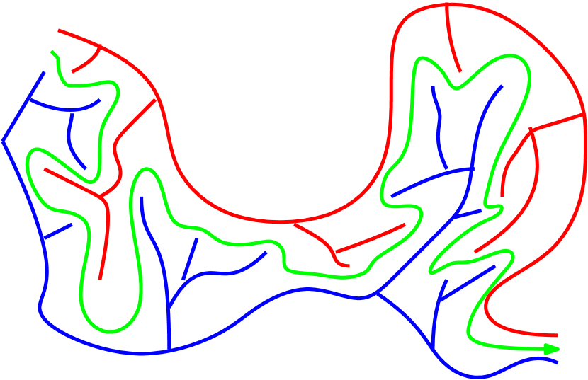
Figure 7: Given an initial portion of the exploration process $\lambda$, the set of active and duplicate edges in the remainder of the graph only depends on the initial segment through its boundary. Consequently, the law of the decorated random map conditional on the part already drawn only depends on the white region with the boundary components consisting in the red and blue curves only visited on one side by the green curve.

Remark 1.9.

There are other notions of “active edge”, each of which gives rise to the same Tutte polynomial

$$T_{M}(x,y)=\sum_{\text{spanning trees $t$ of $M$}}x^{\text{\# internally active edges of $t$}}\,y^{\text{\# externally active edges of $t$}}\,.$$

The embedding activity illustrated in Figure 4 differs from Tutte’s original definition, but is more natural in this context because it has the domain Markov property, and has a simple characterization in terms of the hamburger-cheesburger model. The embedding activity is similar to Bernardi’s definition [bernardi-sandpile, § 3.1, Def. 3], but with “maximal” in place of “minimal”. The partition function $\mathcal{Z}(M,e_{0},y,1)=T_{M}(y,y)$ is the Tutte polynomial of $M$ evaluated at $(y,y)$. In this case ($z=1$), the partition function is that of the active spanning tree model of [kassel-wilson-active], which when $y\geq 1$ coincides with the partition function of the self-dual Fortuin–Kasteleyn (FK) model with parameter $q=(y-1)^{2}$.

Remark 1.10.

To our knowledge, the notion of edges of duplicate type does not appear elsewhere in the literature. However, this notion can be viewed as a variant of the notion of bending energies studied in [bbg-bending] and initially introduced in a different guise in [DiFrancesco]. Suppose $(\mathcal{T},\mathbbm{v})$ is a rooted triangulation and $\ell$ is a non-self-crossing oriented loop in the dual of $\mathcal{T}$, viewed as a cyclically ordered sequence of distinct triangles in $\mathcal{T}$. For each triangle $t$ hit by loop $\ell$, there is a single edge of $t$ which is not shared by the triangles hit by $\ell$ immediately before and after $t$. We say that $t$ points outward (resp. inward) if this edge is on the same (resp. opposite) side of the loop $\ell$ as the root vertex $\mathbbm{v}$. The bending of $\ell$ is the number of pairs of consecutive triangles which either both point outward or both face inward. Such a pair of triangles corresponds to a time when loop $\ell$ “bends around” a vertex. If we view the Peano curve $\lambda$ considered above as a loop in the triangulation whose edges are the union of the edges of the quadrangulation $Q$ and the trees $T$ and $T^{*}$, then the bending of $\lambda$ in the sense of [bbg-bending] is the number of consecutive pairs of symbols of one of the forms ${\mathsf{h}}{\mathsf{h}}$, ${\mathsf{H}}{\mathsf{H}}$, ${\mathsf{h}}{\mathsf{H}}$, ${\mathsf{H}}{\mathsf{h}}$, ${\mathsf{c}}{\mathsf{c}}$, ${\mathsf{C}}{\mathsf{C}}$, ${\mathsf{c}}{\mathsf{C}}$, or ${\mathsf{C}}{\mathsf{c}}$ in the identified word which encodes the triple $(M,e_{0},T)$ under Sheffield’s bijection.

The loops considered in [bbg-bending] are those arising from variants of the $O(n)$ model, so are expected to be non-space-filling in the limit (in fact they are conjectured to converge to CLE${}_{\kappa}$ loops for $\kappa\in(8/3,8)$ [shef-cle]). For space-filling loops (such as the Peano curve $\lambda$), it is natural to keep track of times when the loop returns to a triangle which shares a vertex with one it hits previously, and then bends toward the set of triangles which it has hit more recently.

Let us now be more precise about what this means. It is easy to see from Sheffield’s bijection (and is explained in [chen-fk, § 4.2]) that two edges $\lambda(i)$ and $\lambda(j)$ for $i,j\in[1,2n]_{\mathbbm{Z}}$ share a primal (resp. dual) endpoint if and only if the rightmost hamburger (resp. cheeseburger) in the reduced words $\hyperlink{def-reduce}{\mathcal{R}}(x_{1}\cdots x_{i})$ and $\hyperlink{def-reduce}{\mathcal{R}}(x_{1}\cdots x_{j})$ both correspond to the same burger in the original word $x$, or if these reduced words both have no hamburgers (resp. cheeseburgers). Consequently, an edge of duplicate type can be equivalently defined as an edge $\lambda(i)$ such that $\lambda$ crosses a quadrilateral of $Q$ for the first time at time $i$ and the following is true. Let $v_{i-1}^{0}$ and $v_{i-1}^{1}$ be the endpoints of $\lambda(i-1)$, enumerated in such a way that $\lambda$ hits an edge which shares the endpoint $v_{i-1}^{0}$ for the first time before it hits an edge which shares the endpoint $v_{i-1}^{1}$ for the first time. Then $\lambda$ turns toward $v_{i-1}^{1}$ at time $i$ (cf. Figure 5). From this perspective, a time when $\lambda$ crosses a quadrilateral bisected by an edge of duplicate type can be naturally interpreted as a time when $\lambda$ “bends away from the set of triangles which it has hit more recently”. Hence our model is a probability measure on planar maps decorated by an active spanning tree (in the sense of [kassel-wilson-active]), weighted by an appropriate notion of the bending of the corresponding Peano curve.

The generalized burger model of Section 1.3 encodes a random planar map decorated by an active spanning tree with bending energy. The correspondence between the probability vector $\vec{p}=(p_{\mathsf{F}},p_{\mathsf{S}},p_{\mathsf{d}},p_{\mathsf{e}})\in\mathcal{P}$ and the pair of parameters $(y,z)$ is given by

$$y=\frac{1+p_{\mathsf{F}}-p_{\mathsf{S}}}{1-p_{\mathsf{F}}+p_{\mathsf{S}}}\quad\text{and}\quad z=\frac{1+p_{\mathsf{d}}-p_{\mathsf{e}}}{1-p_{\mathsf{d}}+p_{\mathsf{e}}}\,,$$ (1.11)

i.e.

$$p_{\mathsf{F}}-p_{\mathsf{S}}=\frac{y-1}{1+y}\quad\text{and}\quad p_{\mathsf{d}}-p_{\mathsf{e}}=\frac{z-1}{1+z}\,.$$ (1.12)

To see why this is the case, let $\dot{X}$ be a random word of length $2n$ sampled from the conditional law of $X_{1}\cdots X_{2n}$ given $\{X(1,2n)=\emptyset\}$, where $X$ is the bi-infinite word from Section 1.3 (in the case when $p_{\mathsf{S}}=1$, we allow the last letter of $\dot{X}$ to be a flexible order, since a word whose orders are all ${\mathsf{S}}$’s cannot reduce to the empty word). Let $\dot{X}^{\prime}\colonequals\hyperlink{def-identification}{\mathcal{I}}(\dot{X})$ and let $(M,e_{0},T)$ be the rooted spanning-tree-decorated planar map associated with $\dot{X}^{\prime}$ under the bijection of [shef-burger, § 4.1].

Lemma 1.11.

1. The law of $(M,e_{0},T)$ is that of the uniform measure on edge-rooted, spanning-tree decorated planar maps weighted by $y^{\operatorname{a}(T)}z^{\operatorname{d}(T)}$, with $y$ and $z$ as in (1.11).

2. The conditional law of $T$ given $(M,e_{0})$ is given by the law (1.10); and when $z=1$, the law of $(M,e_{0},T)$ is that of an active-tree-decorated planar map (as defined in the introduction).

3. If $(M^{\infty},e_{0}^{\infty},T^{\infty})$ is the infinite-volume rooted spanning-tree-decorated planar map associated with $X$ (by the infinite-volume version of Sheffield’s bijection, see the discussion just after (1.8)), then $(M^{\infty},e_{0}^{\infty},T^{\infty})$ has the law of the Benjamini-Schramm limit [benjamini-schramm-topology] of the law of $(M,e_{0},T)$ as $n\rightarrow\infty$.

Proof.

Throughout the proof we write $a\propto b$ if $a/b$ is a constant depending only on $n$ and $\vec{p}$. Let $x\in\mathcal{W}(\Theta)$ be a word of length $2n$ which satisfies $\hyperlink{def-reduce}{\mathcal{R}}(x)=\emptyset$. Note that $x$ must contain $n$ burgers and $n$ orders. Then in the notation of Definition 1.4,

$$\mathbbm{P}\!\mathopen{}\mathclose{{}\left(\dot{X}=x}\right)\propto\\ \mathopen{}\mathclose{{}\left(\frac{2p_{\mathsf{F}}}{1-p_{\mathsf{F}}-p_{\mathsf{S}}}}\right)^{\hyperlink{def-theta-count}{\mathcal{N}\!}_{{\mathsf{F}}}(x)}\mathopen{}\mathclose{{}\left(\frac{2p_{\mathsf{S}}}{1-p_{\mathsf{F}}-p_{\mathsf{S}}}}\right)^{\hyperlink{def-theta-count}{\mathcal{N}\!}_{{\mathsf{S}}}(x)}\mathopen{}\mathclose{{}\left(\frac{2p_{\mathsf{d}}}{1-p_{\mathsf{d}}-p_{\mathsf{e}}}}\right)^{\hyperlink{def-theta-count}{\mathcal{N}\!}_{{\mathsf{d}}}(x)}\mathopen{}\mathclose{{}\left(\frac{2p_{\mathsf{e}}}{1-p_{\mathsf{d}}-p_{\mathsf{e}}}}\right)^{\hyperlink{def-theta-count}{\mathcal{N}\!}_{{\mathsf{e}}}(x)}.$$ (1.13)

Let $A^{\mathsf{H}}$ (resp. $\widetilde{A}^{\mathsf{H}}$) be the set of $i\in[1,2n]_{\mathbbm{Z}}$ for which $\dot{X}_{i}^{\prime}$ is a hamburger order matched to a hamburger which is (resp. is not) the rightmost burger in $\dot{X}^{\prime}(1,i-1)$ (notation as in (1.8)). Let $D^{\mathsf{H}}$ (resp. $\widetilde{D}^{\mathsf{H}}$) be the set of $i\in[2,2n]_{\mathbbm{Z}}$ for which $\dot{X}_{i}^{\prime}$ is a hamburger, $\dot{X}^{\prime}(1,i-1)\neq\emptyset$, and the rightmost burger in $\dot{X}^{\prime}(1,i-1)$ is a hamburger (resp. cheeseburger). Define $A^{\mathsf{C}}$, $\widetilde{A}^{\mathsf{C}}$, $D^{\mathsf{C}}$, and $\widetilde{D}^{\mathsf{C}}$ similarly but with hamburgers and cheeseburgers interchanged. Then

$$\operatorname{a}(T)=\#A^{\mathsf{H}}+\#A^{\mathsf{C}}\quad\operatorname{and}\quad\operatorname{d}(T)=\#D^{\mathsf{H}}+\#D^{\mathsf{C}}.$$

If we condition on $\dot{X}^{\prime}$, then we can re-sample $\dot{X}$ as follows. For each $i\in A^{\mathsf{H}}$, independently sample $\dot{X}_{i}\in\{{\mathsf{H}},{\mathsf{F}}\}$ from the probability measure $\mathbbm{P}({\mathsf{H}})=(1-p_{\mathsf{F}}-p_{\mathsf{S}})/(1+p_{\mathsf{F}}-p_{\mathsf{S}})$, $\mathbbm{P}({\mathsf{F}})=2p_{\mathsf{F}}/(1+p_{\mathsf{F}}-p_{\mathsf{S}})$. For each $i\in\widetilde{A}^{\mathsf{H}}$, independently sample $\dot{X}_{i}\in\{{\mathsf{H}},{\mathsf{S}}\}$ from the probability measure $\mathbbm{P}({\mathsf{H}})=(1-p_{\mathsf{F}}-p_{\mathsf{S}})/(1-p_{\mathsf{F}}+p_{\mathsf{S}})$, $\mathbbm{P}({\mathsf{S}})=2p_{\mathsf{S}}/(1-p_{\mathsf{F}}+p_{\mathsf{S}})$. For each $i\in D^{\mathsf{H}}$, independently sample $\dot{X}_{i}\in\{{\mathsf{h}},{\mathsf{d}}\}$ from the probability measure $\mathbbm{P}({\mathsf{h}})=(1-p_{\mathsf{d}}-p_{\mathsf{e}})/(1+p_{\mathsf{d}}-p_{\mathsf{e}})$, $\mathbbm{P}({\mathsf{d}})=2p_{\mathsf{d}}/(1+p_{\mathsf{d}}-p_{\mathsf{e}})$. For each $i\in\widetilde{D}^{\mathsf{H}}$, independently sample $\dot{X}_{i}\in\{{\mathsf{h}},{\mathsf{e}}\}$ from the probability measure $\mathbbm{P}({\mathsf{h}})=(1-p_{\mathsf{d}}-p_{\mathsf{e}})/(1-p_{\mathsf{d}}+p_{\mathsf{e}})$, $\mathbbm{P}({\mathsf{e}})=2p_{\mathsf{e}}/(1-p_{\mathsf{d}}+p_{\mathsf{e}})$. Then do the same for $A^{\mathsf{C}}$, $\widetilde{A}^{\mathsf{C}}$, $D^{\mathsf{C}}$, and $\widetilde{D}^{\mathsf{C}}$ but with hamburgers and cheeseburgers interchanged.

The above resampling rule implies that with $x$ as above,

$$\mathbbm{P}\!\mathopen{}\mathclose{{}\left(\dot{X}=x\,|\,\dot{X}^{\prime}=\hyperlink{def-identification}{\mathcal{I}}(x)}\right) \propto\mathopen{}\mathclose{{}\left(\frac{1-p_{\mathsf{F}}+p_{\mathsf{S}}}{1+p_{\mathsf{F}}-p_{\mathsf{S}}}}\right)^{\operatorname{a}(T)}\mathopen{}\mathclose{{}\left(\frac{1-p_{\mathsf{d}}+p_{\mathsf{e}}}{1+p_{\mathsf{d}}-p_{\mathsf{e}}}}\right)^{\operatorname{d}(T)}\mathopen{}\mathclose{{}\left(\frac{2p_{\mathsf{F}}}{1-p_{\mathsf{F}}-p_{\mathsf{S}}}}\right)^{\hyperlink{def-theta-count}{\mathcal{N}\!}_{{\mathsf{F}}}(x)}$$

$$\qquad\times\mathopen{}\mathclose{{}\left(\frac{2p_{\mathsf{S}}}{1-p_{\mathsf{F}}-p_{\mathsf{S}}}}\right)^{\hyperlink{def-theta-count}{\mathcal{N}\!}_{{\mathsf{S}}}(x)}\mathopen{}\mathclose{{}\left(\frac{2p_{\mathsf{d}}}{1-p_{\mathsf{d}}-p_{\mathsf{e}}}}\right)^{\hyperlink{def-theta-count}{\mathcal{N}\!}_{{\mathsf{d}}}(x)}\mathopen{}\mathclose{{}\left(\frac{2p_{\mathsf{e}}}{1-p_{\mathsf{d}}-p_{\mathsf{e}}}}\right)^{\hyperlink{def-theta-count}{\mathcal{N}\!}_{{\mathsf{e}}}(x)}.$$ (1.14)

By dividing (1.13) by (1.4), we obtain

$$\mathbbm{P}\!\mathopen{}\mathclose{{}\left(\dot{X}^{\prime}=\hyperlink{def-identification}{\mathcal{I}}(x)}\right)\propto y^{\operatorname{a}(T)}z^{\operatorname{d}(T)}.$$

Therefore, the probability of any given realization of $(M,e_{0},T)$ is proportional to $y^{\operatorname{a}(T)}z^{\operatorname{d}(T)}$, which gives assertion 1. Assertion 2 is an immediate consequence of assertion 1. Assertion 3 follows from the same argument used in [shef-burger, § 4.2] together with the results of Appendix LABEL:sec-prelim. ∎

Remark 1.12.

The model described in Lemma 1.11 is self dual in the sense that the law of $(M,e_{0},T)$ is the same as the law of $(M^{*},e_{0}^{*},T^{*})$, where $M^{*}$ is the dual map of $M$, $e_{0}^{*}$ is the edge of $M^{*}$ which crosses $e_{0}$, and $T^{*}$ is the dual spanning tree (consisting of edges of $M^{*}$ which do not cross edges of $T$). This duality corresponds to the fact that the law of the inventory accumulation model of Section 1.3 is invariant under the replacements ${\mathsf{h}}\leftrightarrow{\mathsf{c}}$ and ${\mathsf{C}}\leftrightarrow{\mathsf{H}}$. It may be possible to treat non-self dual variants of this model in our framework by relaxing the requirement that $\mathbbm{P}({\mathsf{h}})=\mathbbm{P}({\mathsf{c}})$ and $\mathbbm{P}({\mathsf{C}})=\mathbbm{P}({\mathsf{H}})$ in (1.7), but we do not investigate this. We remark that there are bijections and Brownian motion scaling limit results analogous to the ones in this paper for other random spanning-tree-decorated map models which do not possess this self duality; see, e.g., [kmsw-bipolar, lsw-schnyder-wood].

We end by recording the following corollary of Lemma 1.11, which says that the law of the identification of the word $X$ (and therefore the law of the associated tree-decorated map) depends on the parmaeter $\vec{p}$ only via the quantities $y$ and $z$ of (1.11).

Corollary 1.13.

Suppose $\vec{p}=(p_{\mathsf{F}},p_{\mathsf{S}},p_{\mathsf{d}},p_{\mathsf{e}})$ and $\widetilde{\mathbbm{P}}=(\widetilde{p}_{\mathsf{F}},\widetilde{p}_{\mathsf{S}},\widetilde{p}_{\mathsf{d}},\widetilde{p}_{\mathsf{e}})$ are two vectors in $\mathcal{P}$ which satisfy $p_{\mathsf{F}}-p_{\mathsf{S}}=\widetilde{p}_{\mathsf{F}}-\widetilde{p}_{\mathsf{S}}$ and $p_{\mathsf{d}}-p_{\mathsf{e}}=\widetilde{p}_{\mathsf{d}}-\widetilde{p}_{\mathsf{e}}$. Let $X=\cdots X_{-1}X_{0}X_{1}\cdots$ (resp. $\widetilde{X}=\cdots\widetilde{X}_{-1}\widetilde{X}_{0}\widetilde{X}_{1}\cdots$) be a bi-infinite word such that $\{X_{i}\}_{i\in\mathbbm{N}}$ (resp. $\{\widetilde{X}_{i}\}_{i\in\mathbbm{N}}$) is a collection of i.i.d. samples from the probability measure (1.7) with probabilities $\vec{p}$ (resp. with $\widetilde{\vec{p}}$). Then the identifications $\hyperlink{def-identification}{\mathcal{I}}(X)$ and $\hyperlink{def-identification}{\mathcal{I}}(\widetilde{X})$ agree in law.

Proof.

It follows from Lemma 1.11 that the infinite-volume tree-decorated planar maps $(M^{\infty},e_{0}^{\infty},T^{\infty})$ and $(\widetilde{M}^{\infty},\widetilde{e}_{0}^{\infty},\widetilde{T}^{\infty})$ associated with $\hyperlink{def-identification}{\mathcal{I}}(X)$ and $\hyperlink{def-identification}{\mathcal{I}}(\widetilde{X})$ agree in law. Since these maps uniquely determine $\hyperlink{def-identification}{\mathcal{I}}(X)$ and $\hyperlink{def-identification}{\mathcal{I}}(\widetilde{X})$, respectively, via the same deterministic procedure, we infer that $\text{<a href="\#def-identification" title="Hy@raisedlink ‣ Definition 1.3. ‣ 1.3 Generalized burger model ‣ 1 Introduction ‣ Active spanning trees with bending energy on planar maps and SLE-decorated Liouville quantum gravity for 𝜅>8" class="ltx\_ref ltx\_font\_italic">I</a>}(X)\stackrel{d}{=}\text{<a href="\#def-identification" title="Hy@raisedlink ‣ Definition 1.3. ‣ 1.3 Generalized burger model ‣ 1 Introduction ‣ Active spanning trees with bending energy on planar maps and SLE-decorated Liouville quantum gravity for 𝜅>8" class="ltx\_ref"><span class="ltx\_text ltx\_ref\_tag">1.3</span></a>}$