Purely imaginary quasinormal modes of the Kerr geometry

Abstract

We present a method for determining the purely imaginary quasinormal modes of the Kerr geometry. Such modes have previously been explored, but we show that prior results are incorrect. The method we present, based on the theory of Heun polynomials, is very general and can be applied to a broad class of problems, making it potentially useful to all branches of physics. Furthermore, our application provides an example where the method of matched asymptotic expansions seems to have failed. A deeper understanding of why it fails in this case may provide useful insights for other situations.

I Introduction

The term Quasinormal Mode (QNM) is often used to describe a natural resonant vibration of an intrinsically dissipative system. While the terminology may vary, the idea is relevant to virtually all branches of physics (cf RefsSettimi et al. (2009); Ge and Hughes (2014); Pan et al. (2015); Tournier and Smith (2003)). The fundamental idea is that, while waves may leave the system, they may not enter the system. For black holes in asymptotically flat spaces, waves may leave the system by flowing into the black hole or by radiating to infinity. Represented by a complex frequency $\omega$, the mode’s real part corresponds to the angular frequency and the imaginary part to the decay rate. The formalism used to understand these modes is straightforwardKokkotas and Schmidt (1999), but subtleties can occur.

The existence and nature of gravitational QNMs of the Kerr geometry on the Negative Imaginary Axis (NIA) have been poorly understood for quite some time. Early numerical studies lacked the accuracy necessary to study QNMs near the NIALeaver (1985); Onozawa (1997), but general arguments suggested that QNMs might not exist on the NIAOnozawa (1997). The studies published to date have found modes near the NIA in the neighborhood of the algebraically special modes of SchwarzschildChandrasekhar (1984) at $\bar{\omega}\equiv M\omega=-2i,-10i,-30i,\ldots$Leaver (1985); Onozawa (1997); Berti et al. (2003). And recent, high-accuracy numerical workCook and Zalutskiy (2014) has shown that some of these QNMs exist arbitrarily close to the NIA near $\bar{\omega}=-2i$. Maassen van den BrinkMaassen van den Brink (2000) showed that the $s=-2$ algebraically special modes of Schwarzschild are simultaneously QNMs and left Total Transmission Modes (TTM_Ls), finally proving that, at least in the zero angular momentum limit (ie. the Schwarzschild limit), a set of QNMs do exist precisely on the NIA. More recently, analytic and numerical work by Yang et alYang et al. (2013) has suggested that a continuum of purely imaginary QNMs exist for polar modes ($m=0$) near the extremal limit of the angular momentum $\bar{a}\equiv a/M\to 1$. Inspired by this work, HodHod (2013) derived a related, but more tailored analytic description of these modes that also imposed the small frequency limit $|\bar{\omega}|\ll 1$.

Using our high-accuracy code for constructing sequences of QNMsCook and Zalutskiy (2014) of Kerr, parameterized by the angular momentum $\bar{a}$, we have constructed many full sequences with much higher overtones than have been previously explored. In doing this we have found numerous additional examples of sequences that approach the NIA at non-vanishing values of $\bar{a}$. In fact, for polar modes, we have found numerous sequences that approach the NIA not simply once, but thousands of times. These occur when a sequence exhibits a looping behavior where the path of the QNMs becomes tangent to the NIA (see Fig. 1 for an example where loops touch the NIA 7 times). We have studied all of these cases with high accuracy and precision.

However, we do not find QNMs on or near the NIA in the vicinity of the numerical results reported by Yang et al, nor do we find results that are in agreement with the analytic work of Hod. To understand these discrepancies, and to fully understand the nature of QNMs on the NIA, we have made a careful study of the behavior of modes of Kerr on the NIA making use of the theory of Heun polynomialsRonveaux (1995). We find two key results. First, we find that QNMs can exist on the NIA only if they correspond to polynomial solutions. Furthermore, $m\neq 0$ QNMs can only exist on the NIA if they have frequency $\bar{\omega}=\bar{\omega}_{\mathchar 45\relax}$ (see Eq. (12)). We have found no examples with $m\neq 0$ that have a QNM on the NIA. For example, in Fig. 1 the $\{2,1,8_{0,1}\}$ and $\{2,2,8_{0,1}\}$ sequences all terminate arbitrarily close to, but not on, the NIA at a non-vanishing value of $\bar{a}$. Second, we find that there are three classes of polynomial solutions on the NIA, each a countably infinite set. One class is part of the known extension of the algebraically special modes of Schwarzschild to cases of non-vanishing $\bar{a}$Chandrasekhar (1984). These modes are plotted in Fig. 2 as solid circles. The first 2 solid black circles correspond to the terminations of $\{2,0,8_{0}\}$ and $\{2,0,9_{0}\}$ on the NIA in Fig. 1. Each of these modes is simultaneously a QNM and a TTM_L. In fact, this class of solutions adds a previously unknown branch to the algebraically special modes of Kerr. The second class of modes are a previously unknown set of QNMs of Kerr. These modes are plotted in Fig. 2 as solid triangles. The first 2 solid black triangles correspond to the terminations of $\{2,0,8_{1}\}$ and $\{2,0,9_{1}\}$ on the NIA in Fig. 1. The third class of modes at first glance appear to be QNMs, but on careful inspection we find that they exhibit both incoming and outgoing waves at the event horizon and are neither QNMs nor TTM_Ls. These modes are plotted in Fig. 2 as faint open squares. Each looping sequence of QNMs that becomes tangent to the NIA (see Fig. 1), touches the axis at exactly one of these frequencies. However, there are an infinite number of this third class of modes that do not correspond to a point on any QNM sequence.

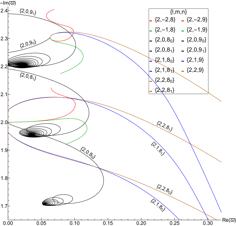
Figure 1: The $n=8$ and 9 overtones of the $\ell=2$ gravitational ($s=-2$) modes of the Kerr geometry. The curves are parameterized by $\bar{a}$. Note that for $n=8$, the $m=1$ and 2 modes are both multiplets that approach arbitrarily close to the NIA. The $m=0$ modes of both overtones are also multiplets, and we show four cases where these modes terminate on the NIA. The $\{2,0,9_{1}\}$ mode becomes tangent to the NIA at 7 locations. None of these 7 points are QNMs.

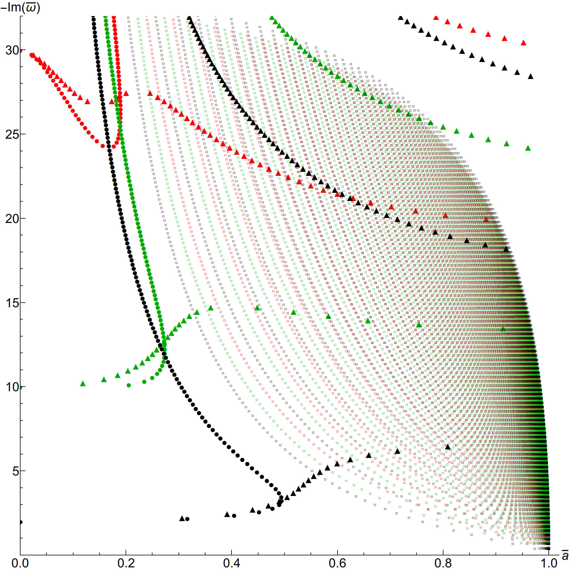
Figure 2: Polynomial solutions for $\ell=2$, 3, and 4. The solid circles are “anomalous” solutions, and so are simultaneously QNMs and TTM_Ls. The solid triangles are QNMs. And the faint open squares are “miraculous” solutions that do not represent any kind of mode. $\ell=2$ modes are in black, $\ell=3$ in green, and $\ell=4$ in red. Note the horizontal axis is $\bar{a}$, not ${\rm Re}(\bar{\omega})$

II Modes on the NIA

The Teukolsky master equations describe the dynamics of a massless field ${}_{s}\psi$ of spin-weight $s$ in the Kerr geometry,

$${}_{s}\psi(t,r,\theta,\phi)=e^{-i\omega{t}}e^{im\phi}S(\theta)R(r).$$ (1)

The angular and radial functions, $S(\theta)$ and $R(r)$ respectively, are obtained by solving a coupled pair of equations, each of which is of the confluent Heun form. Written in nonsymmetrical canonical form, the confluent Heun equation reads

$$\frac{d^{2}H(z)}{dz^{2}}+\left(4p+\frac{\gamma}{z}+\frac{\delta}{z-1}\right)\frac{dH(z)}{dz}+\frac{4\alpha pz-\sigma}{z(z-1)}H(z)=0,$$ (2)

with regular singular points at $z=0,1$ and an irregular singular point at $z=\infty$. Frobenius solutions local to each of the three singular points can be defined in terms of two functionsRonveaux (1995),

$$Hc^{(a)}(p,\alpha,\gamma,\delta,\sigma;z) =\sum_{k=0}^{\infty}{c^{(a)}_{k}z^{k}},$$ (3)

$$Hc^{(r)}(p,\alpha,\gamma,\delta,\sigma;z) =\sum_{k=0}^{\infty}{c^{(r)}_{k}z^{-\alpha-k}}.$$ (4)

We are usually interested in solutions called confluent Heun functions which are simultaneously Frobenius solutions for two adjacent singular points. However, in this work, polynomial solutions will play an important role. Confluent Heun polynomials are simultaneously Frobenius solutions of all three singular points.

The radial Teukolsky equation can be placed into nonsymmetrical canonical form by making the transformation

$$R(z)=z^{\eta}(z-1)^{\xi}e^{(r_{+}-r_{\mathchar 45\relax})\zeta z}H(z),$$ (5)

where $r_{\pm}$ are the radii of the event and Cauchy horizons and $z\equiv\frac{r-r_{\mathchar 45\relax}}{r_{+}-r_{\mathchar 45\relax}}$. See Ref.Cook and Zalutskiy (2014); Borissov and Fiziev (2010) for a complete description. The parameters $\xi$, $\eta$, and $\zeta$ can each take on one of two values allowing for a total of eight ways to achieve nonsymmetrical canonical form. We will focus on the particular cases where

$$\begin{array}[]{r}\zeta=i\omega\equiv\zeta_{+},\\ \xi=-s-i\sigma_{+}\equiv\xi_{\mathchar 45\relax},\end{array}\quad\mbox{with}\quad\sigma_{+}\equiv\frac{2\bar{\omega}r_{+}-ma}{r_{+}-r_{\mathchar 45\relax}}.$$ (6)

The choice of $\xi=\xi_{\mathchar 45\relax}$ means that the local solution at the horizon ($z=1$) given by

$$Hc^{(a)}(-p,\alpha,\delta,\gamma,\sigma-4p\alpha;1-z)$$ (7)

represents waves traveling into the black hole, while $\zeta=\zeta_{+}$ means the local solution given by Eq. (4) represents waves traveling out at $z\to\infty$. These are the boundary conditions appropriate for QNMs. The two possible choices for $\eta=\eta_{\pm}$ correspond to two possible local behaviors at the Cauchy horizon $z=0$ and are relevant to the polynomial solutions below.

II.0.1 Solutions as confluent Heun functions

The majority of QNM solutions are found in the form of confluent Heun functions. These are readily found using “Leaver’s method”Leaver (1985, 1986) which consists of removing the asymptotic behavior via $H(z)=z^{-\alpha}\bar{R}(z)$ and rescaling the radial coordinate as $z\to\frac{z-1}{z}$ so the relevant domain is $0\leq z\leq 1$. The solution is expanded as $\bar{R}(z)=\sum_{n=0}^{\infty}{a_{n}z^{n}}$. The series has a radius of convergence of one and more precisely, with $r_{n}\equiv\frac{a_{n+1}}{a_{n}}$,

$$\lim_{n\to\infty}r_{n}=1+\frac{u_{1}}{\sqrt{n}}+\frac{u_{2}}{n}+\frac{u_{3}}{n^{\frac{3}{2}}}+\cdots,$$ (8)

and

$$\lim_{n\to\infty}a_{n}\propto n^{u_{2}}e^{2u_{1}\sqrt{n}}.\vspace*{-4pt}$$ (9)

There will be two independent series solutions to the recurrence relation. The QNM solutions we seek will be a minimal solution we denote by $a_{n}\to f_{n}$, and we label the other set of coefficients by $a_{n}\to g_{n}$. A minimal solution has the property that $\lim_{n\to\infty}{\frac{f_{n}}{g_{n}}}=0$. With $u_{1}=\pm\sqrt{-2i(r_{+}-r_{\mathchar 45\relax})\omega}$, the sign choice corresponds to the two possible asymptotic behaviors for $a_{n}$. So long as ${\rm Re}(\omega)\neq 0$ a minimal solution may exist. The ratio $r_{n}$ can be written as a continued fraction in terms of the coefficients of the recurrence relation for the $a_{n}$. The key property of this recurrence relation is given by Pincherle’s theoremGautschi (1967) which states that the continued fraction $r_{0}$ converges if and only if the series expansion has a minimal solution $a_{n}=f_{n}$ with $f_{0}\neq 0$. The continued fraction $r_{0}$ must converge to a specific value, and so QNM solutions are found at those frequencies $\omega$ where $r_{0}$ does converge to the required value.

But, it is very important to recognize that for $\omega$ on the NIA, $\lim_{n\to\infty}\frac{f_{n}}{g_{n}}$ becomes oscillatory and a minimal solution cannot exist unless the infinite series solution terminates. Thus, any QNM solution on the NIA must be of the form of a confluent Heun polynomial. Furthermore, the continued fraction cannot be used to determine the QNM frequencies $\bar{\omega}$ on the NIA.

II.0.2 Polynomial solutions

Because confluent Heun polynomials are simultaneous Frobenius solutions of all three singular points, they can be represented in several different ways. To avoid confusion, consider the local solution around the event horizon at $z=1$ given by Eq. (7). The local Heun solution $Hc^{(a)}(p,\alpha,\gamma,\delta,\sigma;z)$ is defined by the three-term recurrence relation

$$0= f^{(a)}_{k}c^{(a)}_{k+1}+g^{(a)}_{k}c^{(a)}_{k}\!+h^{(a)}_{k}c^{(a)}_{k-1}\ :\begin{array}[]{l}c^{(a)}_{-1}=0,\\ c^{(a)}_{0}=1,\end{array}$$ (10c)

$$g^{(a)}_{k}= k(k-4p+\gamma+\delta-1)-\sigma,$$ (10d)

$$f^{(a)}_{k}= -(k+1)(k+\gamma),$$ (10e)

$$h^{(a)}_{k}= 4p(k+\alpha-1).$$ (10f)

For the series to terminate with order $q$ (a non-negative integer), two conditions must be satisfiedRonveaux (1995). First, the lower diagonal element $h^{(a)}_{q+1}$ must vanish which requires $\alpha=-q$. The second condition, denoted by $\Delta_{q+1}=0$, is that the determinant of the $(q+1)\times(q+1)$ matrix of recurrence coefficients must vanish:

$$\left|\begin{array}[]{ccccc}g_{0}&f_{0}&0&\cdots&0\\ h_{1}&g_{1}&f_{1}&\ddots&0\\ 0&h_{2}&g_{2}&\ddots&0\\ 0&0&\ddots&\ddots&\ddots\\ 0&0&\cdots&h_{q}&g_{q}\end{array}\right|=0.$$ (11)

The first necessary condition for a polynomial solution to exist, $\alpha=-q$, can be satisfied in one of two ways:

$$\bar{\omega}=\bar{\omega}_{+}\!\equiv\frac{\bar{a}m-iN_{+}\sqrt{1-\bar{a}^{2}}}{2(1+\sqrt{1-\bar{a}^{2}})}\ \ \mbox{or}\ \ \bar{\omega}=\bar{\omega}_{\mathchar 45\relax}\!\equiv-i\frac{N_{\mathchar 45\relax}}{4},$$ (12)

where $N_{\pm}$ are integers. These two possibilities are associated with the two independent local behaviors at the Cauchy horizon ($z=0$). Choosing either family of possible solutions and fixing a value for $N_{\pm}$, a sufficient condition for the existence of a polynomial solution is to find a root of the $\Delta_{q+1}=0$ condition considered as a function of the angular momentum $\bar{a}$. There is, however, one very important caveat.

We must be careful to examine, for each regular singular point, the behavior of the roots of the indicial equation. At the event horizon ($z=1$), the two roots are $0$ and $1-\delta$. Frobenius theory tells us that, for regular singular points, if the roots of the indicial equation differ by an integer or zero, in general only one series solution exists corresponding to the larger root. A similar condition holds for irregular singular points, but is not important for this problem.

For the family of solutions associated with $\bar{\omega}_{\mathchar 45\relax}$ we have encountered no instances where $\delta$ is an integer. This means that polynomial solutions of this family are QNMs. However the $\bar{\omega}_{+}$ family of solutions is of a form that guarantees $\delta$ is a negative integer. In this case, we find two possibilities. The first is that the only series solution behaves like $(z-1)^{1-\delta}$ instead of $(z-1)^{0}$. A solutions of this kind is referred to as “anomalous”Maassen van den Brink (2000) and represents a solution that is simultaneously a QNM and a TTM_L. The other possibility is that the $(z-1)^{0}$ solution persists. Solutions of this kind are referred to as “miraculous”Maassen van den Brink (2000) and we will show that they do not represent a mode of any kind. These behaviors are, to say the least, counter-intuitive.

II.0.3 Anomalous and miraculous solutions

Standard Frobenius theory tells us that when the roots of the indicial equation differ by an integer, only the local series solution corresponding to the larger root is guaranteed to exist. The second local solution will usually include a $\log$ term. However, it is possible for the coefficient multiplying this $\log$ term to vanish. To understand the implications of these two possibilities for our problem, it is useful to view them from the perspective of scattering theory.

Consider the “anomalous” case. Begin with an outgoing mode and then construct an nth-order Born approximation as a function of $\omega$. We find starting at a certain order in the series, the denominator contains a term that vanishes when $\bar{\omega}=\bar{\omega}_{+}$. Essentially, this means that scattering by the potential is so strong that the normally dominant behavior of the outgoing wave is overwhelmed and the outgoing wave has exactly the same local behavior as the incoming wave. See Ref. Maassen van den Brink (2000) for a more rigorous discussion of this.

In terms of Heun polynomials, when $-\delta$ is an integer less than $q=-\alpha$, then the upper-diagonal coefficient $f^{(a)}_{-\delta}$ vanishes. This means that the determinant of the tri-diagonal matrix, Eq. (11), can be written as the product of the determinants of the two diagonal block elements where the blocks are split following the $1-\delta$ row and columnEl-Mikkawy (2004). Note that the upper off-diagonal block contains all zeros, and the lower off-diagonal block contains one non-zero element, $h^{(a)}_{1-\delta}$ which cannot vanish. In the case of an “anomalous” solution, it is the determinant of the lower diagonal block that vanishes. This means that the first $1-\delta$ expansion coefficients vanish and the leading-order behavior of the Heun polynomial will be $(z-1)^{1-\delta}$.

For the “miraculous” case, we find that it is the determinant of the upper diagonal block that vanishes. Returning momentarily to the example of the Born approximation of the outgoing mode, we find that the vanishing denominator is countered by a vanishing numerator and in the limit this term in the Born series is finite. Again, see Ref. Maassen van den Brink (2000) for a more rigorous discussion. This “miraculous” coincidence is the same miracle that causes the coefficient of the $\log$ term to vanish in the context of general Frobenius theory, and is guaranteed by the vanishing of the determinant of the upper diagonal block in the case of confluent Heun polynomials.

The subtlety of the “miraculous” case stems from the fact that the limiting value of the coefficient of the $(z-1)^{1-\delta}$ term in the expansion of the Born approximation is not the same as the coefficient of this term in the Heun polynomial solution. In short, the local behavior of the Heun polynomial solution at $z=1$ is a linear combination of the local behaviors of an incoming and an outgoing wave. Given the polynomial solution, we can explicitly construct a linearly independent solution with the same $\bar{a}$ and $\bar{\omega}$. This solution has the behavior of an incoming wave at $z=1$ potentially allowing us to subtract away this unwanted contribution from the polynomial solution. However, it behaves like an incoming wave at infinity as well, so we cannot fix the behavior at one boundary without spoiling it at the other. Thus, these “miraculous” solutions are neither QNMs nor TTM_Ls.

III Summary and Discussion

The approach we have described allows for a complete determination of the QNMs of the Kerr geometry on the NIA. For the case of gravitational perturbations $s=-2$ we have compared our results to QNMs in the neighborhood of the NIA that were obtained with high numerical accuracy. In all three classes described above, we find the limiting behavior of the numerical results to be in precise agreement with the frequency $\bar{\omega}$ and angular momentum $\bar{a}$ associated with the polynomial solutions. The agreement spans more than a thousand instances and at times required numerical results computed to an accuracy of $10^{-12}$ or better to accurately distinguish between possible solutions.

We have shown that there are many solutions that are clearly QNMs on the NIA ($\bar{\omega}_{\mathchar 45\relax}$), and many that are simultaneously QNMs and TTM_Ls on the NIA (anomalous cases of $\bar{\omega}_{+}$). In fact, it seems clear that there should be a countably infinite set of both such modes. We have also shown that a third class of polynomial solutions (miraculous cases of $\bar{\omega}_{+}$) are not QNMs even though on first inspection they would appear to satisfy the required criteria. Additional details on the methods to find these modes and their interesting behavior will be discussed in a future paperCook and Zalutskiy (2016)

The numerical solutions for QNMs on the NIA found in Ref. Yang et al. (2013) used Leaver’s method for finding QNMs as the roots of a continued fraction. While the majority of their numerical solutions are valid, we have shown that this method cannot be used to find QNMs on the NIA and their solutions on the NIA are not valid. Yet these misidentified QNMs appear in good agreement with the analytic approximations in Refs. Yang et al. (2013) and Hod (2013). First, we note that Hod’s analytic description of these “QNMs” (see Eq. (21) of Ref. Hod (2013)) takes a form identical to our $\bar{\omega}_{+}$ condition. The important difference, using our notation, is that his modes require $N_{+}$ be near to, but explicitly not, an integer. Furthermore, he finds a nearby total reflection mode (a TTM_L in our terminology). It is possible that Hod’s solutions result from a “splitting of the exact solution” caused by the various approximations that were made. It is also likely that the matched asymptotic expansions used in these worksYang et al. (2013); Hod (2013) are forcing a general solution to apply in a situation where only a polynomial solution is allowed. A deeper understanding of why these analytic methods fail in this special situation might be very helpful for numerous other situations.