Structural analysis of high-dimensional basins of attraction

Abstract

We propose an efficient Monte Carlo method for the computation of the volumes of high-dimensional bodies with arbitrary shape. We start with a region of known volume within the interior of the manifold and then use the multi-state Bennett acceptance-ratio method to compute the dimensionless free-energy difference between a series of equilibrium simulations performed within this object. The method produces results that are in excellent agreement with thermodynamic integration, as well as a direct estimate of the associated statistical uncertainties. The histogram method also allows us to directly obtain an estimate of the interior radial probability density profile, thus yielding useful insight into the structural properties of such a high dimensional body. We illustrate the method by analysing the effect of structural disorder on the basins of attraction of mechanically stable packings of soft repulsive spheres.

I Introduction

In science we often face, and occasionally confront, the following question: “Can we estimate the a priori probability of observing a system in a very unlikely state?” An example is: “How likely is a given disordered sphere packing?”, not to mention questions such as “How likely is life, or the existence of a universe like ours?” within the context of dynamical systems and of the multiverse. In a number of cases, where the states correspond to extrema in a high dimensional function, this question can be narrowed down to: “How large is the ‘basin of attraction’ of a given state?”. In such cases, estimating the probability of observing a particular state is equivalent to computing the volume of the (high-dimensional) basin of attraction of this state. That simplifies the problem, but not by much Ball (1997); Simonovits (2003): analytical approaches are typically limited to highly symmetric (often convex) volumes, whilst ‘brute force’ numerical techniques can deal with more complex shapes, but only in low-dimensional cases. Computing the volume of an arbitrary, high-dimensional body is extremely challenging. For instance, it can be proved that the exact computation of the volume of a convex polytope is a NP-hard problem Dyer and Frieze (1988); Khachiyan (1989, 1988) and, of course, the problem does not get any easier in the non-convex case.

Yet, the importance of such computations is apparent: the volume of the basin of attraction for the extrema of a generic energy landscape, be that of biological molecules Miller and Wales (1999), an artificial neural network Sagun et al. (2014); Ballard et al. (2016a, b), a dynamical system Wiley et al. (2006); Menck et al. (2013), or even of a “string theory landscape” (where the minima corresponds to different de Sitter vacua Frazer and Liddle (2011); Greene et al. (2013)), is essential for understanding the systems’ behavior.

In high dimensions, simple quadrature and brute-force sampling fail Bishop (2009) and other methods are needed. In statistical mechanics, the problem is equivalent to the calculation of the partition function (or, equivalently, the free energy) of a system, and several techniques have been developed to tackle this problem (see e.g Frenkel and Smit (2002)). The earliest class of techniques to compute partition functions is based on thermodynamic integration (TI) Kirkwood (1935); Gelman and Meng (1998); Frenkel and Smit (2002), which is based on the idea that a transformation of the Hamiltonian of the system can transform an unknown partition function into one that is known analytically. More recent techniques include histogram-based methods (Wang-Landau Wang and Landau (2001), parametric and non parametric weighted histogram analysis method (WHAM) Habeck (2012)) or Nested Sampling Skilling (2004); Martiniani et al. (2014). In essence, all these techniques reduce the computation of the partition function to the numerical evaluation of a one-dimensional integral.

Among the above methods Nested Sampling and Wang Landau are Monte Carlo algorithms in their own right, that produce the (binned) density of states as a by-product. On the other hand, TI can be identified as a particular Umbrella Sampling scheme Frenkel and Smit (2002), that outputs multiple sets of equilibrium states that can be analysed, either by numerical quadrature (e.g. see the Einstein crystal method Frenkel and Ladd (1984)), or by WHAM and multi-state Bennet acceptance ratio method (MBAR). All the above methods can be used to compute high-dimensional volumes. However, the choice of the MBAR method Shirts and Chodera (2008) is an optimal one. Not only is MBAR non-parametric (no binning is required) and has the lowest known variance reweighting estimator for free energy calculations, but it also eliminates the need for explicit numerical integration of the density of states, thus reducing to a minimum the number of systematic biases.

One reason why brute force methods are not suited to estimate the volumes of high-dimensional bodies, is that for such bodies the volume of the largest inscribed hypersphere, quickly becomes negligible to the volume of the smallest circumscribed hypersphere – and most of the volume of the circumscribed hypersphere is empty. Hence, using a Monte Carlo ‘rejection method’ to compute the volume of the non-convex body as the fraction of volume contained in a hypersphere Liu et al. (2007); Ashwin et al. (2012), does not yield accurate results: the largest contribution should come from points that are barely sampled, if at all.

In this Letter we show that MBAR can be used, not only to arrive at an accurate estimate of a high-dimensional, non-convex volume, but that it also can be used to probe the spatial distribution of this volume.

II Computing High-Dimensional Volumes

Our aim is then to measure the volume of a $n-\text{dimensional}$ connected compact manifold $\Omega\subseteq\mathbb{R}^{n}$ with boundaries. We require this body to be “well guaranteed”, i.e. it has both an inscribed and a circumscribed hypersphere Simonovits (2003). To explore different parts of the non-convex volume, we use a spherically symmetric bias that either favors the sampling of points towards the center, or towards the periphery. We start by performing a series of $K+1$ random walks under different applied bias potentials, similarly to the Einstein-crystal method Frenkel and Ladd (1984). We refer to each of the walkers as a “replica” $R_{i}$. Unlike TI, where biasing is always ‘attractive’ (i.e. it favors larger confinement), in MBAR we are free to choose both attractive and repulsive bias potentials (see SM for details of our implementation). Additionally MBAR uses the full posterior distribution (hence all moments) rather than just the average log-likelihood computed over the posterior, as for TI. The present method directly yields an estimate for the statistical uncertainty in the results that depends on the full distributions and is sensitive to their degree of overlap, thus making the method more robust to under-sampling. In contrast, TI would require an expensive resampling numerical procedure to achieve the same objective.

The Markov Chain Monte Carlo (MCMC) random walk of replica $i\in[0,K]$ will generate samples with unnormalised probability density $q_{i}(\mathbf{x})$, which for a standard Metropolis Monte Carlo walk is

$$q_{i}(\mathbf{x})\equiv e^{-\beta_{i}U_{i}(\mathbf{x})}$$ (1)

with biasing potential $U_{i}(\mathbf{x})$ and inverse temperature $\beta_{i}$; from now on we assume $\beta_{i}=1$ for all walkers $R_{i}$, without loss of generality. The normalised probability density is then

$$p_{i}(\mathbf{x})=Z_{i}^{-1}q_{i}(\mathbf{x})$$ (2)

with normalisation constant

$$Z_{i}=\int_{\mathbb{R}^{n}}q_{i}(\mathbf{x})\mathop{}\!\mathrm{d}\mathbf{x}.$$ (3)

We require that the bias potential $U_{i}(\mathbf{x})$ can be factorised as

$$U_{i}(\mathbf{x})=\mathbf{\raisebox{0.0pt}[4.30554pt][4.30554pt]{$\chi$}}_{\Omega}(\mathbf{x})u_{i}(\mathbf{x})$$ (4)

where $u_{i}$ is the reduced potential function and $\mathbf{\raisebox{0.0pt}[4.30554pt][4.30554pt]{$\chi$}}_{\Omega}(\mathbf{x})$ is the “oracle” Simonovits (2003), such that for all choices of $u_{i}(\mathbf{x})$,

$$U_{i}(\mathbf{x})=\left\{\begin{array}[]{l l}u_{i}(\mathbf{x})&\quad\text{if $\mathbf{x}\in\Omega$}\\ \infty&\quad\text{if $\mathbf{x}\not\in\Omega$}\end{array}\right.\$$ (5)

We thus have that the normalisation constant in Eq. (3) becomes an integral over the manifold $\Omega$

$$Z_{i}=\int_{\mathbb{R}^{n}}e^{-U_{i}(\mathbf{x})}\mathop{}\!\mathrm{d}\mathbf{x}=\int_{\Omega}e^{-u_{i}(\mathbf{x})}\mathop{}\!\mathrm{d}\mathbf{x}.$$ (6)

If replica $R_{M}$ is chosen to have bias $u_{M}=0$, by definition Eq. (6) becomes the volume $V_{\Omega}$. Hence if we can compute the partition function for the reduced potential function $u_{M}=0$, we can compute the volume $V_{\Omega}$.

The MBAR method Shirts and Chodera (2008) is a binless and statistically optimal estimator to compute the difference in dimensionless free energy for multiple sets of equilibrium states (trajectories) $\{\mathbf{x}\}_{i}$ obtained using different biasing potentials $u_{i}(\mathbf{x})$. The difference in dimensionless free energy is defined as

$$\Delta\hat{f}_{ij}\equiv\hat{f}_{j}-\hat{f}_{i}=-\ln\left(\frac{Z_{j}}{Z_{i}}\right)$$ (7)

which can be computed by solving a set of self-consistent equations as described in Ref. Shirts and Chodera (2008). Note that only the differences of the dimensionless free energies are meaningful as the absolute values $\hat{f}_{i}$ are determined up to an additive constant and that the “hat” indicates MBAR estimates for the dimensionless free energies, to be distinguished from the exact (reference) values.

Let us define the volume $V_{\omega}=\pi^{n/2}r_{\omega}^{n}/\Gamma(n/2+1)$ of a $n$-ball $\omega\subseteq\Omega$ with radius $r_{\omega}$ centred on $\mathbf{x}_{0}$ and absolute dimensionless free energy $f_{\omega}=-\ln V_{\omega}$. For instance, when the volume of a basin of attraction in a potential energy landscape is to be measured, $\mathbf{x}_{0}$ is chosen to be the minimum energy configuration and $\omega\subseteq\Omega$ the largest $n$-ball centred at $\mathbf{x}_{0}$ that fits in $\Omega$. We also define $\{\mathbf{x}\}_{i}$ to be the set of states sampled with biasing potential $u_{i}$ and $\{\mathbf{x}\}_{\omega}=\cup_{i=0}^{K}\{\mathbf{x}:|\mathbf{x}-\mathbf{x}_{0}|\leq r_{\omega}\}_{i}$ to be the set of states re-sampled within $\omega$ with reduced potential

$$u_{\omega}(\mathbf{x})=\left\{\begin{array}[]{l l}0&\quad\text{if $|\mathbf{x}-\mathbf{x}_{0}|\leq r_{\omega}$}\\ \infty&\quad\text{if $|\mathbf{x}-\mathbf{x}_{0}|>r_{\omega}$}\end{array}\right.\$$ (8)

In other words we augment the set of states with the additional reduced potential $u_{\omega}$. Note that MBAR can compute free energy differences and uncertainties between sets of states not sampled (viz. with a different reduced potential function) without any additional iterative solution of the self-consistent estimating equations, see Ref. Shirts and Chodera (2008) for details.

Computing the free energy difference between the sets of equilibrium states $\{\mathbf{x}\}_{\omega}$ and $\{\mathbf{x}\}_{M}$, chosen to have reduced potentials $u_{M}=0$ and $u_{\omega}$, we find that the absolute free energy for the unbiased set of states $\{\mathbf{x}\}_{M}$ is

$$f_{M}=f_{\omega}+(\hat{f}_{M}-\hat{f}_{\omega})$$ (9)

where the free energy difference $\hat{f}_{M}-\hat{f}_{\omega}$ is obtained by MBAR with associated uncertainty $\delta\Delta\hat{f}_{M\omega}$. The volume of the manifold is then just $V_{\Omega}=\exp(-f_{M})$ with uncertainty $\delta V_{\Omega}=V_{\Omega}\delta\Delta\hat{f}_{M\omega}$. Note that the set of biasing potentials $u_{i}$ must be chosen so that there is sufficient overlap between each neighbouring pair of $p_{i}(\mathbf{x})$. For instance for the harmonic bias $u_{i}=k_{i}|\mathbf{x}-\mathbf{x}_{0}|^{2}/2$ we must choose a set of coupling constants $k_{i}$ so that all neighbouring replicas have a sufficient probability density overlap.

Under an appropriate choice of biasing potential the present method may yield information such as the radial posterior probability density function, as an easy to compute by-product, details are discussed in the SM.

III Basins of attraction in high dimensions

We define a basin of attraction as the set of all points that lead to a particular minimum energy configuration by a path of steepest descent on a potential energy surface (PES). Exploring a basin of attraction is computationally expensive because each call to the oracle function $\mathbf{\raisebox{0.0pt}[4.30554pt][4.30554pt]{$\chi$}}_{\Omega}(\mathbf{x})$ requires a full energy minimisation and equilibrating a MCMC on a high dimensional support is difficult Xu et al. (2011); Asenjo et al. (2013, 2014); Martiniani et al. (2016). For this reason little is known about the geometry of these bodies Xu et al. (2010); Wang et al. (2012); Asenjo et al. (2013); Martiniani et al. (2016).

Ashwin et al. Ashwin et al. (2012), defined the basin of attraction as the collection of initial zero-density configurations that evolve to a given jammed packing of soft repulsive disks via a compressive quench. On the basis of ‘brute-force’ calculations on low-dimensional systems, Ashwin et al. suggested that basins of attraction tend to be “branched and threadlike” away from a spherical core region. However, the approach of ref. Ashwin et al. (2012) breaks down for higher dimensional systems for which most of the volume of the basin is concentrated at distances from the ‘minimum’ where the overwhelming majority of points do not belong to the basin. The method that we present here allows us to explore precisely those very rarified regions where most of the ‘mass’ of a basin is concentrated.

In general the representation of all high dimensional convex bodies should have a hyperbolic form such as the one proposed in the illustration by Ashwin et al. due to the exponential decay in volume of parallel hypersections (slices) away from the median (or equator) Milman (1998). This holds true even for the simplest convex bodies, such as the hypercube, and the underlying geometry need not be “complicated”, as one would guess at first from the two-dimensional representation. For the simplest cases of the unit $d$-sphere and the unit $d$-cube it can be shown that most of the volume is contained within $\mathcal{O}(1/d)$ of the boundary and that at the same time the volume is contained in a slab $\mathcal{O}(1/\sqrt{d})$ and $\mathcal{O}(1)$ from the equator, irrespective of the choice of north pole, respectively Ball (1997); Guruswami and Kannan (2012). Hence, there is virtually no interior volume. Such phenomena of concentration of measure are ubiquitous in high dimensional geometry and are closely related to the law of large numbers Guruswami and Kannan (2012).

As we will show, the results presented by Ashwin et al. are, within the resolution available to their method, qualitatively consistent with those for a simple (unit) hypercube.

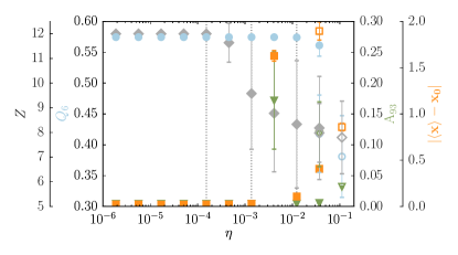
Figure 1: Structural disorder as a function of polydispersity $\eta$ is quantified by the average coordination number $Z$ (grey diamonds) and the $Q_{6}$ bond orientational order parameter (blue circles); error bars correspond to one standard deviation of the distribution of values per particle. Basin shape is characterized by the asphericity factor $A_{d}$ (green triangles) and the mean distance of the centre of mass from the minmum (orange squares); error bars correspond to the standard error. Filled and empty markers correspond to packings obtained starting from an fcc and a disordered arragement respectively. Dotted lines show the $\eta$ after which, in order, $Z$, $A_{d}$ and $Q_{6}$ change from the fcc value.

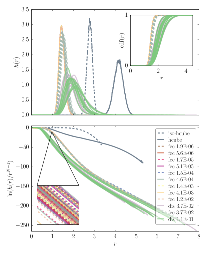
Figure 2: Top plot shows the measured basin radial probability density function $h(r)$ (DOS) for packings at different polydispersities. The solid and dashed blue curves correspond to the DOS of a $93$D hypercube, measured from the centre of mass (‘iso-cube’) and from a point in one of the corners. The top inset shows the cumulative distribution function for $h(r)$. The bottom panel shows the logarithm of the ratio of the DOS of the basin and of a $93$D hyperball. The bottom inset shows the set of barely distinguishable overlapping curves measured for low polydispersities. Top and bottom plots share the x-axis.

III.1 Effect of structural disorder on the basins of attraction of jammed sphere packings

We characterise the basins of attraction for a number of 32 hard-core plus soft-shell three-dimensional sphere packings, analogous to the ones described in Ref. Martiniani et al. (2016). The soft shell interactions are short ranged and purely repulsive, the full functional form of the potential and further technical details are reported in the SM. We systematically introduce structural disorder by preparing packings with (geometrically) increasing particle size polydispersity $\eta$, i.e. the (positive) radii are sampled from a normal distribution $\mathcal{N}(1,\eta)$. For each $\eta$ we prepare $\sim$10 packings at a soft packing fraction $\phi=0.74148$ with a soft to hard-sphere radius ratio of $r_{\mathrm{SS}}/r_{\mathrm{HS}}=1.12$. The particles are placed initially in a fcc arrangement $\mathbf{x}_{\text{fcc}}$ and then relaxed via an energy minimisation to a mechanically stable state $\mathbf{x}_{0}$. Thus, for the lowest polydispersities the packings remain in a perfect fcc structure and with increasing $\eta$ they progressively move away into a disordered glassy state. For the largest polydispersity, for which hard-core overlaps do not allow an initial fcc arrangement, we sample a series of completely random initial states followed by an energy minimisation. Note that even for $\eta\approx 0$, due to the high packing fraction, starting from a completely random set of coordinates, an energy minimisation does not lead to the fcc crystal but rather to the closest glassy state (inherent structure). We are interested in the effect of structural disorder on the shape of the basin of attraction for the soft sphere packings.

We determine the amount of structural disorder in the packing by computing the $Q_{6}$ bond orientational order parameter Steinhardt et al. (1983) and the average number of contacts per particle $Z$, shown in Fig. 1. As the polydispersity of the system is increased, the coordination number $Z$ decays monotonically from the close-packed value of $12$ to a value $Z_{\mathrm{fcc}}>Z>Z_{\mathrm{iso}}$, where $Z_{\mathrm{iso}}=6$ is the average contact number at iso-staticity for a three-dimensional packing of frictionless spheres O’Hern et al. (2003). The $Q_{6}$ order parameter, computed using a solid-angle based nearest-neighbor definition van Meel et al. (2012), decays from its fcc value well after the contact number has dropped below the close-packed value of $12$.

We start characterising the shape of the high dimensional basins of attraction associated with these packings by performing an unconstrained random walk within the basin and performing principal component analysis (PCA) on the trajectory thus obtained Bishop (2009). PCA yields a set of eigenvectors that span the $d$-dimensional configurational space with associated eigenvalues $\lambda_{1},\dots,\lambda_{d}$. If the basin posses $d$-dimensional spherical symmetry then all the eigenvalues are expected to be equal. A measure of the shape of a random walk is then the asphericity factor Rudnick and Gaspari (1987)

$$A_{d}=\frac{\sum_{i>j}(\lambda_{i}-\lambda_{j})^{2}}{(d-1)\left(\sum_{i=1}^{d}\lambda_{i}\right)^{2}},$$ (10)

that has a value of $0$ for a spherically symmetric random walk and of $1$ for a walk that extends only in one dimension. Furthermore, we compute the distance of the centre of mass (CoM) position from the minimum energy configuration for the random walk, $|\langle\mathbf{x}\rangle-\mathbf{x}_{0}|$. This quantity reveals whether the basin is isotropic around the minimum or not. Both quantities, averaged over all packings, are plotted as a function of polydispersity in Fig. 1 along with the structural order parameters. Interestingly, we observe that for low $\eta$ the basins are, on average, spherically symmetric and isotropic around the minimum. With the onset of structural disorder we observe a marginal increase in asphericity and in the CoM distance from the minimum. In order to observe a significant change however, we need to go to the fully disordered packings at higher polydispersity. With increasing polydispersity, we observe significant changes in the structural order parameters and in the asphericity factor $A_{d}$ and CoM distance from the minimum.

The implementation details of the MBAR method that we have used are discussed in the SM. Using this method to compute the volume of the basins of attraction, we find excellent agreement with thermodynamic integration, see Fig. S2. As a natural by-product of the computation we are able to compute the radial probability density function (DOS), shown in Fig. 2 together with the logarithm of the ratio between the measured DOS, and that of a $d$-hypersphere. The log-ratio curves clearly show that all basins have a well-defined hyperspherical core region, where the curves are flat around $0$, followed by a series of exponential decays at larger distances from the minimum. For $\eta<10^{-4}$ the curves are mostly indistinguishable from one another with most of the probability mass concentrated between $1<r<3$, as it can be seen from the inset showing the corresponding cumulative distribution function (CDF). For higher polydispersity, the DOS curves have ever longer tails, as it is also shown by the systematic shift in the CDF.

Importantly, the curves show that a ‘rejection’ method to measure the basin volume will fail. In this method, the volume of the basin is determined by integrating the fraction of points on a hyper-shell with radius $r$ that fall inside the basin. That fraction is the function shown in the bottom panel of Fig. 2. The most important contribution to the integral would come from the range of $r$ values where $h(r)$ (top panel of Fig. 2) has a significant value. As can be seen from the figure, for disordered systems this happens for values of $r$ where the fraction of hyper-sphere points within the basin is extremely small, in the example shown $\mathcal{O}(10^{-30})$. Hence, the dominant part of the integral would come from parts that are never sampled.

To interpret our results for the DOS curves, it is useful to compare with the corresponding result for a unit hypercube (see Fig. 2). In one instance we do so by placing the ‘origin’ of the hypercube at its CoM, and in another by placing the origin on one of the $2^{d}$ corners of the hypercube, to generate a DOS of a system with a very anisometric density distribution. Not surprisingly, moving the origin of the system from the center to the corner of a hypercube has a dramatic effect on the shape of the DOS, which is now much more similar to the curves for large $\eta$, with similar characteristic changes of slope observed for the basins. Again, this agrees with the observation that the CoM distance increases with increasing structural disorder. The effect of the basin asphericity, as measured by the asphericity factor $A_{d}$ is difficult to infer from the DOS alone.

We thus observe that the structural isotropy and high degree of rotational symmetry in the crystal, as indicated by the $Q_{6}$ parameter, is reflected in the isotropy and spherical symmetry of the basin around the minimum, even for relatively large polydispersities when the average contact number has already dropped considerably from the close-packed value. Similarly, the structural disorder at larger $\eta$ is reflected in the anisotropy and asphericity of the basin. Hence, changes in the basin structure, as indicated by the asphericity factor, the $CoM$ and the density profile, occur before any observable changes occur in $Q_{6}$ and after the average contact number ($Z\lesssim 9$) has fallen well below the close-packed value of $12$.