Cavity quantum interferences with three-level atoms

Abstract

We discuss quantum interference phenomena in a system consisting from a laser driven three-level ladder-type emitter possessing orthogonal transition dipoles and embedded in a leaking optical resonator. The cavity mean-photon number vanishes due to the destructive nature of the interference phenomena. The effect occurs for some particular parameter regimes which were identified. Furthermore, upper bare-state population inversion occurs as well.

I Introduction

Quantum interference effects involving various atomic transition amplitudes were intensively investigated recently agw ; ficek ; martin . It originate from indistinguishability of the corresponding transition pathways. As a consequence, quenching of spontaneous emission occurs due to quantum interference effects between decaying pathways which are dependent on mutual orientation of corresponding transition dipoles chk1 . Laser- or phase-control of spontaneous emission processes were demonstrated there. Also, quantum interference effects lead to very narrow spectral lines in the spontaneous emission spectrum of pumped molecular, semiconductor or highly charged ion systems chk2 . Furthermore, such spontaneously generated coherences in a large ensemble of nuclei operating in the x-ray regime and resonantly coupled to a common cavity environment were experimentally demonstrated in je . Previously it was shown that multi-level atoms interacting with the vacuum of a preselected cavity mode, in the bad-cavity limit, exhibit cavity induced quantum interference which is similar to the spontaneously generated coherences due to parallel transition dipoles knight . Quantum interference effects in an ensemble of ${}^{229}{\rm Th}$ nuclei interacting with coherent light were demonstrated too, in Ref. aaa . Destructive or constructive interference effects were observed even in a strongly pumped few-level quantum- dot sample njp ; viorel . Protection of bipartite entanglement das or continuous variable entanglement gx via quantum interferences were shown to occur as well. Finally, electromagnetic induced transparency is an another phenomenon of quantum destructive interference which makes a resonant opaque medium highly transparent and dispersive within a narrow spectral band eit .

Based on this background, here, we study the quantum dynamics of a three-level ladder-type atomic system possessing orthogonal transition dipoles and embedded in an optical leaking resonator. The atomic sample is pumped coherently and resonantly with external electromagnetic field sources. Despite of photon scattering into surrounding electromagnetic modes including the cavity one and resonant laser-atom driving, we identify regimes when the cavity mode is empty in the good-cavity limit. We demonstrate that this occurs due to destructive quantum interference effects among the involved transition pathways. The effect is maximal when the cavity mode frequency is in resonance with particular resonance fluorescence sidebands. This is distinct from interference phenomena observed in je where the experiment was performed in the bad-cavity limit and different parameter regimes. Furthermore, most upper bare-state population inversion is achieved as well in our system although it is identified with coherent population trapping effects rather than quantum interference phenomena which lead to zero cavity mean-photon numbers. The inversion can facilitate the generation of correlated or entangled photon-pairs when one photon lies in an optical range while another one is in a higher frequency domain, i.e., EUV or X ray etc.

The article is organized as follows. In Section II we describe the Hamiltonian, the adopted approximations and the master equation describing our system. In Section III we discuss and analyze the obtained results. The Summary is given in Section IV.

II Theoretical framework

We consider a laser driven three-level $\Sigma\rm{-type}$ atom placed in a cavity of frequency $\omega_{c}$ and leaking rate $\kappa$. We denote via $\omega_{32}$ the transition frequency from the most excited level $|3\rangle$ to the intermediate level $|2\rangle$ whereas $\omega_{21}$ is the frequency of the transition from the state $|2\rangle$ to the ground state $|1\rangle$. The atom’s decay rates via spontaneous emissions corresponding to each transition are defined as $\gamma_{32}$ and $\gamma_{21}$, respectively. The atomic system is coherently pumped, perpendicularly to the cavity axis, by two different laser fields of frequencies $\omega_{L1}$ and $\omega_{L2}$ with $\Omega_{1}$ and $\Omega_{2}$ being the corresponding Rabi frequencies on transitions $|2\rangle\leftrightarrow|1\rangle$ and $|3\rangle\leftrightarrow|2\rangle$ (see Fig. 1). Correspondingly, the cavity-atom interaction constants are given by $g_{1}$ and $g_{2}$. The Hamiltonian describing the whole system is:

$$H = \hbar\omega_{c}a^{\dagger}a+\hbar\sum^{3}_{i=1}\omega_{i}S_{ii}+i\hbar g_{1}(a^{\dagger}S_{12}-S_{21}a)$$ (1)

$$+ i\hbar g_{2}(a^{\dagger}S_{23}-S_{32}a)+\hbar\Omega_{1}(S_{21}e^{-i\omega_{L1}t}+S_{12}e^{i\omega_{L1}t})$$

$$+ \hbar\Omega_{2}(S_{32}e^{-i\omega_{L2}t}+S_{23}e^{i\omega_{L2}t}).$$

Here $S_{ij}=|i\rangle\langle j|$, $\{i,j=1,2,3\}$, are the atom operators, while $\{a^{\dagger},a\}$ are the cavity field creation and annihilation operators and obey the commutation relations $[S_{\alpha,\beta},S_{\beta^{\prime},\alpha^{\prime}}]=\delta_{\beta,\beta^{\prime}}S_{\alpha,\alpha^{\prime}}-\delta_{\alpha^{\prime},\alpha}S_{\beta^{\prime},\beta}$ and $[a,a^{\dagger}]=1$, respectively. The first two terms in Eq. (1) describe the single mode free cavity field and the atom free Hamiltonians. The external laser fields and the cavity field interact with both transitions of the atom and every interaction is defined via separate terms corresponding to each transition. Thus, the next two terms of the Hamiltonian represent the interaction of the quantized cavity with the atom whereas the last two terms describe the laser-atom semi-classical interaction.

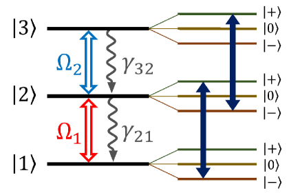
Figure 1: (color online) Schematic of the model. A three-level atom, placed in a leaking optical cavity, interacts with external coherent fields with $\Omega_{2,1}$ being the corresponding Rabi frequencies. $\gamma_{32}$ and $\gamma_{21}$ are the respective spontaneous emission decay rates. The full arrows depict the dressed-state transitions in resonance with the cavity mode frequency leading to cavity quantum interference phenomena.

The system’s quantum dynamics is given by the master equation for the density operator $\rho$ as:

$$\frac{\partial\rho}{\partial t} = -\frac{i}{\hbar}[H,\rho]+\frac{\kappa}{2}\mathcal{L}(a)+\frac{\gamma_{32}}{2}\mathcal{L}(S_{23})+\frac{\gamma_{21}}{2}\mathcal{L}(S_{12}),$$

where, on the right-hand side of the equation, the first term represents the coherent evolution based on the system Hamiltonian $H$, while the other terms describe the damping phenomena, i.e., the cavity field damping and the spontaneous emissions processes, respectively. The damping effects are expressed by the Liouville superoperator $\mathcal{L}$, which acts on a given operator $\mathcal{O}$ as: $\mathcal{L}(\mathcal{O})=2\mathcal{O}\rho\mathcal{O}^{\dagger}-\mathcal{O}^{\dagger}\mathcal{O}\rho-\rho\mathcal{O}^{\dagger}\mathcal{O}$.

In the usual interaction picture with $\omega_{L1}=\omega_{L2}\equiv\omega_{L}$ it is more convenient to apply the semi-classical dressed-state transformation defined as:

$$|1\rangle = -\frac{1}{\sqrt{2}}\cos{\theta}\,|-\rangle-\sin{\theta}\,|0\rangle+\frac{1}{\sqrt{2}}\cos{\theta}\,|+\rangle,$$

$$|2\rangle = \frac{1}{\sqrt{2}}\,|-\rangle+\frac{1}{\sqrt{2}}\,|+\rangle,$$

$$|3\rangle = -\frac{1}{\sqrt{2}}\sin{\theta}\,|-\rangle+\cos{\theta}\,|0\rangle+\frac{1}{\sqrt{2}}\sin{\theta}\,|+\rangle,$$ (3)

with $\theta=\arccos{(\Omega_{1}/\Omega)}$ and $\Omega=\sqrt{\Omega_{1}^{2}+\Omega_{2}^{2}}$. Then, in the dressed-state picture, the system’s dynamics is described by the following dressed-state master equation:

$$\frac{\partial\rho}{\partial t} = -\frac{i}{\hbar}[H,\rho]+\frac{\kappa}{2}\mathcal{L}(a)+\frac{\gamma_{32}\cos^{2}{\theta}}{4}(\mathcal{L}(R_{-0})+\mathcal{L}(R_{+0}))$$ (4)

$$+ \frac{\gamma_{32}\sin^{2}{\theta}+\gamma_{21}\cos^{2}{\theta}}{8}(\mathcal{L}(R_{z})+\mathcal{L}(R_{+-})$$

$$+ \mathcal{L}(R_{-+}))+\frac{\gamma_{21}\sin^{2}{\theta}}{4}(\mathcal{L}(R_{0-})+\mathcal{L}(R_{0+})).$$

Here, the secular approximation was performed in the spontaneous emission terms by neglecting the time-dependent rapidly oscillating terms - an approximation valid as long as $\gamma_{32(21)}/\Omega\ll 1$. The dressed-state atomic operators $R_{ij}=|i\rangle\langle j|$, $\{i,j\}\in\{-,0,+\}$, and $R_{z}=R_{++}-R_{--}$, obey the same commutation relations as the old ones. The system Hamiltonian in the dressed-state picture is expressed as:

$$H = \hbar\delta_{c}a^{\dagger}a+\hbar\Omega R_{z}+\{\frac{i}{2}(g_{1}\cos{\theta}+g_{2}\sin{\theta})a^{\dagger}R_{z}$$ (5)

$$+ \frac{i}{2}(g_{1}\cos{\theta}-g_{2}\sin{\theta})a^{\dagger}(R_{+-}-R_{-+})$$

$$- \frac{i}{\sqrt{2}}g_{1}\sin{\theta}\,a^{\dagger}(R_{0-}+R_{0+})$$

$$- \frac{i}{\sqrt{2}}g_{2}\cos{\theta}\,a^{\dagger}(R_{-0}+R_{+0})\}+\rm{H.c.}\},$$

with $\delta_{c}=\omega_{c}-\omega_{L}$.

As a next step, we perform a unitary transformation: $U(t)=\exp\{itH_{0}/\hbar\}$ where $H_{0}=\hbar\delta_{c}a^{\dagger}a+\hbar\Omega R_{z}$ to arrive at the following transformed Hamiltonian:

$$H = \frac{i}{2}(g_{1}\cos{\theta}-g_{2}\sin{\theta})a^{\dagger}e^{i\delta_{c}t}(R_{+-}e^{2i\Omega t}-R_{-+}e^{-2i\Omega t})$$ (6)

$$- \frac{i}{\sqrt{2}}g_{1}\sin{\theta}\,a^{\dagger}e^{i\delta_{c}t}(R_{0-}e^{i\Omega t}+R_{0+}e^{-i\Omega t})$$

$$- \frac{i}{\sqrt{2}}g_{2}\cos{\theta}\,a^{\dagger}e^{i\delta_{c}t}(R_{-0}e^{-i\Omega t}+R_{+0}e^{i\Omega t})$$

$$+ \frac{i}{2}(g_{1}\cos{\theta}+g_{2}\sin{\theta})a^{\dagger}e^{i\delta_{c}t}R_{z}+\rm{H.c.}.$$

Analyzing the Hamiltonian one can conclude that the atom’s resonance fluorescence spectra on each transition is formed of sidebands centered at $\omega_{L}\pm\Omega$ and $\omega_{L}\pm 2\Omega$ as well as a central peak around $\omega_{L}$. The dressed-state Hamiltonian significantly simplifies if one tunes the laser-cavity detuning $\delta_{c}$ in resonance with one of the sidebands frequency. In what follows, we shall consider such a situation when $\omega_{c}=\omega_{L}+2\Omega$, i.e. $\delta_{c}=2\Omega$ (notice that similar results would be obtained for a cavity tuned to the lowest energy sideband, i.e., when $\delta_{c}=-2\Omega$). In this case, the dressed-state Hamiltonian is

$$H=ig(a^{\dagger}R_{-+}-R_{+-}a),$$ (7)

with $g=\frac{1}{2}(g_{2}\sin{\theta}-g_{1}\cos{\theta})$. This Hamiltonian accurately describes the quantum dynamics within the adopted approximations as long as $g_{1,2}/\Omega\ll 1$. Furthermore, the obtained Hamiltonian has a similar form to the Hamiltonian of a two-level atom interacting with a cavity with an effective coupling $g$. This effective coupling originates from the quantum interference of the two dressed-state transition amplitudes, see Fig. (1), contributing to the atom pumping of the cavity mode. As it will be shown later, it is possible to configure the two Rabi frequencies in order to effectively decouple the atom from the cavity, i.e., the effective coupling vanishes when $g_{1}/g_{2}=\Omega_{2}/\Omega_{1}$. Correspondingly, the cavity mode is empty, although the pumped atom spontaneously scatters photons. Notice that when $\delta_{c}=\{0,\pm\Omega\}$ there are no destructive quantum interference effects.

The master equation (4), with the Hamiltonian (7), is solved by projecting into the system’s states basis hf . The first projection in the atom’s dressed-state basis leads to a set of five linearly coupled differential equations defined by the variables: $\rho^{(0)}=\rho_{--}+\rho_{00}+\rho_{++}$, $\rho^{(1)}=\rho_{++}+\rho_{--}$, $\rho^{(2)}=\rho_{++}-\rho_{--}$, $\rho^{(3)}=(a^{\dagger}\rho_{+-}+\rho_{-+}a)/2$, and $\rho^{(4)}=(\rho_{+-}a^{\dagger}+a\rho_{-+})/2$, where $\rho_{ij}=\langle i|\rho|j\rangle$, $\{i,j\in-,0,+\}$, namely,

$$\dot{\rho}^{(0)} = -2g(\rho^{(4)}-\rho^{(3)})+\frac{\kappa}{2}\mathcal{L}_{0}(a),$$

$$\dot{\rho}^{(1)} = -2g(\rho^{(4)}-\rho^{(3)})+\frac{\kappa}{2}\mathcal{L}_{1}(a)-\frac{\alpha}{2}\rho^{(1)}+\gamma_{32}\cos^{2}{\theta}\rho^{(0)},$$

$$\dot{\rho}^{(2)} = -2g(\rho^{(4)}+\rho^{(3)})+\frac{\kappa}{2}\mathcal{L}_{2}(a)-\frac{\beta}{2}\rho^{(2)},$$

$$\dot{\rho}^{(3)} = \frac{g}{4}(2a^{\dagger}(\rho^{(2)}+\rho^{(1)})a+a^{\dagger}a(\rho^{(2)}-\rho^{(1)})+(\rho^{(2)}-\rho^{(1)})$$

$$\times a^{\dagger}a)-\zeta\rho^{(3)}+\frac{\kappa}{2}(\mathcal{L}_{3}(a)+\rho^{(3)}-2\rho^{(4)}),$$

$$\dot{\rho}^{(4)} = \frac{g}{4}(2a(\rho^{(2)}-\rho^{(1)})a^{\dagger}+aa^{\dagger}(\rho^{(2)}+\rho^{(1)})+(\rho^{(2)}+\rho^{(1)})$$ (8)

$$\times aa^{\dagger})-\zeta\rho^{(4)}+\frac{\kappa}{2}(\mathcal{L}_{4}(a)-\rho^{(4)}).$$

Here $\alpha=\gamma_{21}\sin^{2}{\theta}+2\gamma_{32}\cos^{2}{\theta}$, $\beta=\gamma_{21}+\gamma_{32}\sin^{2}{\theta}$ and $\zeta=(\gamma_{21}(2+\cos^{2}{\theta})+3\gamma_{32}\sin^{2}{\theta})/4$. The next projection in the field’s basis leads to a set of infinite equations corresponding to the infinite Fock states $\{|n\rangle,n\in\mathcal{N}\}$, that is,

$$\dot{P}^{(0)}_{n} = -2g(P_{n}^{(4)}-P_{n}^{(3)})+\kappa(n+1)P_{n+1}^{(0)}-\kappa nP_{n}^{(0)},$$

$$\dot{P}^{(1)}_{n} = -2g(P_{n}^{(4)}-P_{n}^{(3)})+\kappa(n+1)P_{n+1}^{(1)}-(\kappa n+\alpha/2)P_{n}^{(1)}$$

$$+ \gamma_{32}\cos^{2}{\theta}P_{n}^{(0)},$$

$$\dot{P}^{(2)}_{n} = -2g(P_{n}^{(4)}+P_{n}^{(3)})+\kappa(n+1)P_{n+1}^{(2)}-(\kappa n+\beta/2)P_{n}^{(2)},$$

$$\dot{P}^{(3)}_{n} = gn(P_{n-1}^{(1)}-P_{n}^{(1)}+P_{n-1}^{(2)}+P_{n}^{(2)})/2-\kappa P_{n}^{(4)}$$

$$+ \kappa(n+1)P_{n+1}^{(3)}-(\kappa(n-1/2)+\zeta)P_{n}^{(3)},$$

$$\dot{P}^{(4)}_{n} = g(n+1)(P_{n+1}^{(2)}+P_{n}^{(2)}-P_{n+1}^{(1)}+P_{n}^{(1)})/2$$ (9)

$$+ \kappa(n+1)P_{n+1}^{(4)}-(\kappa(n+1/2)+\zeta)P_{n}^{(4)},$$

where $P_{n}^{(i)}=\langle n|\rho^{(i)}|n\rangle$. Interestingly, $P_{n}^{(0)}$ are the diagonal elements of the field’s reduced density matrix, i.e., it contains the trace over the atom’s dressed-states: $P_{n}^{(0)}=\langle n|Tr_{atom}[\rho]|n\rangle$. Hence, it is possible to deduce the cavity field’s mean photon number $\langle n\rangle$ by tracing over the the field’s states:

$$\langle n\rangle=\langle a^{\dagger}a\rangle=\sum_{n=0}^{\infty}nP_{n}^{(0)}.$$ (10)

Respectively, the second order photon-photon correlation function $g^{(2)}(0)$ is given by:

$$g^{(2)}(0)=\frac{\langle a^{\dagger}a^{\dagger}aa\rangle}{\langle n\rangle^{2}}=\frac{\sum_{n=0}^{\infty}n(n-1)P_{n}^{(0)}}{\langle n\rangle^{2}}.$$ (11)

After some mathematical manipulations one finds:

$$\langle R_{\pm\pm}\rangle=\sum_{n=0}^{\infty}(P_{n}^{(1)}\pm P_{n}^{(2)})/2,$$ (12)

with the condition $\langle R_{++}\rangle+\langle R_{00}\rangle+\langle R_{--}\rangle=1$. Using also transformation (3), the population of the upper bare state is given by:

$$\langle S_{33}\rangle=\cos^{2}{\theta}+(1-3\cos^{2}{\theta})\sum_{n=0}^{\infty}P_{n}^{(1)}/2.$$ (13)

Finally, in order to solve the infinite system of Eqs. (9), we truncate it at a certain maximum value $n=N_{max}$ of considered Fock states. The photon distribution of the field converges to zero for larger $N_{max}$, and thus, $N_{max}$ is selected such that a further increase of its value does not modify the obtained results.

III Results and Discussion

The mean cavity photon number as well as their quantum statistics are shown in Fig. (2). A dip in the photon number is clearly visible when $g_{1}/g_{2}=\Omega_{2}/\Omega_{1}$. It is due to quantum interference effects with a destructive nature on the cavity field photons. The interference occurs because both dressed-state transitions of the atom are coupled to the cavity mode leading to indistinguishable photon emission (see also Fig. 1). A destructive quantum interference phenomenon is observed when the cavity is tuned to one of the external sidebands, i.e., $\omega_{c}=\omega_{L}\pm 2\Omega$. Respectively, the atom decouples from the cavity field in this particular case. Thus, the zero cavity photon detection in this scheme is directly related to quantum interference phenomena. Quantum switching devises are feasible applications here, because, the mean-photon number abruptly changes from zero to a particular value which depends on the atom-cavity coupling. The photon statistics shows super-Poissonian behaviors. Particularly, $g^{(2)}(0)\to 2$ and $\langle n\rangle\to 0$ when $\Omega_{2}/\Omega_{1}=g_{1}/g_{2}$. Here, the involved parameters or their ratios can be determined when the cavity mean- photon number vanishes. Additional applications may be related to quantum networks where tools to control the involved processes are highly required kimble .

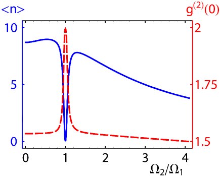
Figure 2: (color online) The quantum steady-state behaviors of the cavity mean photon number $\langle n\rangle$ (solid curve) as well as of the second-order photon-photon correlation function $g^{(2)}(0)$ (dashed line) as a function of the ratio of the two Rabi frequencies $\Omega_{2}/\Omega_{1}$. Here, $\gamma_{32}=\gamma_{21}\equiv\gamma$, $g_{1}/\gamma=5.001$, $g_{2}/\gamma=5$ and $\kappa/\gamma=10^{-3}$.

Fig. 3 shows the bare-state population of the upper state $|3\rangle$ as well as the cavity mean-photon number when $\gamma_{32}\ll\gamma_{21}$ while $\omega_{32}=\omega_{L2}$ and $\omega_{21}=\omega_{L1}$ with $\omega_{L1}\not=\omega_{L2}$. The cavity mode resonantly couples with the upper atomic transition $|3\rangle\leftrightarrow|2\rangle$ only, i.e. $g_{1}=0$. This situation is described as well by the analytical formalism developed here via setting $g_{1}=0$ in Eqs. (9). Reasonable population inversion is achieved. We have found that the inversion is a signature of the coherent population trapping phenomenon tq , i.e., the atom is trapped in the dressed-state $|0\rangle=\cos{\theta}|3\rangle-\sin{\theta}|1\rangle$. Then with a suitable chose of the ratio $\Omega_{2}/\Omega_{1}$ one can transfer the populations among the state $|3\rangle\leftrightarrow 1\rangle$. Furthermore, the cavity field does not affect the bare-state population dynamics in the adopted approximations. As a concrete atomic system, for this particular configuration, one may consider He atoms, $\{3^{1}S,2^{1}P_{1},1^{1}S_{0}\}$ scully . The spontaneous decay rates ratio is approximately $\gamma_{32}/\gamma_{21}\approx 10^{-2}$. The corresponding transition wavelengths are $\lambda_{32}=728.3{\rm nm}$ and $\lambda_{21}=58.4{\rm nm}$. Instead of a continuous wave laser on the high-frequency transition one may consider a long pulse laser wave. Potential applications here may be related to entangled photon pair emissions sczb in optical and EUV (or even higher) frequency ranges.

IV Summary

Summarizing, we have investigated the quantum dynamics of a three-level atom embedded in an optical cavity and resonantly interacting with external coherent electromagnetic waves. We have found parameter regimes where the atom completely decouples from the interaction with the cavity field. As a consequence, the cavity mean photon number goes to zero. Photon vanishing is due to quantum interference effects involving two possible dressed-state atomic transitions. Their indestinguishability leads to destructive quantum interference phenomena. Upper bare-state population inversion occurs as well.

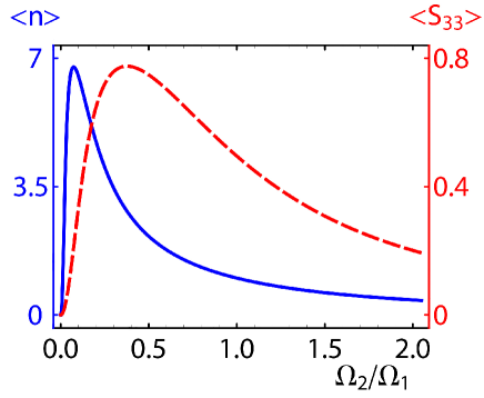
Figure 3: (color online) The steady-state evolution of the cavity mean photon number $\langle n\rangle$ (solid line) and the upper bare-state population $\langle S_{33}\rangle$ (dashed curve) as a function of $\Omega_{2}/\Omega_{1}$. Here, $\gamma_{32}/\gamma_{21}=10^{-2}$, $g_{2}/\gamma_{21}=5$, $\kappa/\gamma_{21}=10^{-3}$.

References

• (1) G. S. Agarwal, Quantum Statistical Theories of Spontaneous Emission and their Relation to other Approaches, (Springer, Berlin, 1974).
• (2) Z. Ficek and S. Swain, Quantum Interference and Coherence: Theory and Experiments, (Springer, Berlin, 2005).
• (3) M. Kiffner, M. Macovei, J. Evers, and C. H. Keitel, Vacuum-Induced Processes in Multilevel Atoms, Progress in Optics 55, 85 (2010).
• (4) S.-Y. Zhu and M. O. Scully, Spectral Line Elimination and Spontaneous Emission Cancellation via Quantum Interference, Phys. Rev. Lett. 76, 388 (1996); M. A. G. Martinez, P. R. Herczfeld, C. Samuels, L.M. Narducci, and C. H. Keitel, Quantum interference effects in spontaneous atomic emission: Dependence of the resonance fluorescence spectrum on the phase of the driving field, Phys. Rev. A 55, 4483 (1997); E. Paspalakis and P. L. Knight, Phase Control of Spontaneous Emission, Phys. Rev. Lett. 81, 293 (1998).
• (5) C. H. Keitel, Narrowing Spontaneous Emission without Intensity Reduction, Phys. Rev. Lett. 83, 1307 (1999); O. Postavaru, Z. Harman, and C. H. Keitel, High-Precision Metrology of Highly Charged Ions via Relativistic Resonance Fluorescence, Phys. Rev. Lett. 106, 033001 (2011).
• (6) K. P. Heeg, H.-C. Wille, K. Schlage, T. Guryeva, D. Schumacher, I. Uschmann, K. S. Schulze, B. Marx, T. Kämpfer, G. G. Paulus, R. Röhlsberger, and J. Evers, Vacuum-Assisted Generation and Control of Atomic Coherences at X-Ray Energies, Phys. Rev. Lett. 111, 073601 (2013).
• (7) B. M. Garraway, and P. L. Knight, Cavity modified quantum beats, Phys. Rev. A 54, 3592 (1996); A. Patnaik, and G. S. Agarwal, Cavity-induced coherence effects in spontaneous emissions from preselection of polarization, Phys. Rev. A 59, 3015 (1999).
• (8) S. Das, A. Pálffy, and C. H. Keitel, Quantum interference effects in an ensemble of ${}^{229}{\rm Th}$ nuclei interacting with coherent light, Phys. Rev. C 88, 024601 (2013).
• (9) B. D. Gerardot, D. Brunner, P. A. Dalgarno, K. Karrai, A. Badolato, P. M. Petroff, and R. J. Warburton, Dressed excitonic states and quantum interference in a three-level quantum dot ladder system, New Journal of Physics 11, 013028 (2009).
• (10) V. Ciornea, M. A. Macovei, Cavity-output-field control via interference effects, Phys. Rev. A 90, 043837 (2014).
• (11) S. Das, G. S. Agarwal, Protecting bipartite entanglement by quantum interferences, Phys. Rev. A 81, 052341 (2010).
• (12) Z.-h. Tang, G.-x. Li, and Z. Ficek, Entanglement created by spontaneously generated coherence, Phys. Rev. A 82, 063837 (2010).
• (13) S. E. Harris, Electromagnetically Induced Transparency, Phys. Today 50, 36 (1997); M. Fleischhauer, A. Imamoglu, and J. P. Marangos, Electromagnetically induced transparency: Optics in coherent media, Rev. Mod. Phys. 77, 633 (2005); Y. Sun, Y. Yang, H. Chen, Sh. Zhu, Dephasing-Induced Control of Interference Nature in Three-Level Electromagnetically Induced Transparency System, Sci. Rep. 5, 16370 (2015).
• (14) T. Quang, and H. Freedhoff, Atomic population inversion and enhancement of resonance fluorescence in a cavity, Phys. Rev. A 47, 2285 (1993).
• (15) H. J. Kimble, The quantum internet, Nature (London) 453, 1023 (2008).
• (16) N. N. Bogolubov Jr., T. Quang, and A. S. Shumovsky, Double optical resonance in a system of atoms, Phys. Lett. A 112, 323 (1985).
• (17) P. K. Jha, A. A. Svidzinsky, and M. O. Scully, Coherence enhanced transient lasing in XUV regime, Laser Phys. Lett. 9, 368 (2012).
• (18) M. O. Scully and M. S. Zubairy, Quantum Optics, (Cambridge University Press, Cambridge, UK, 1997).