Statistical investigation and thermal properties for a 1-D impact system with dissipation

Abstract

The behavior of the average velocity, its deviation and average squared velocity are characterized using three techniques for a 1-D dissipative impact system. The system – a particle, or an ensemble of non interacting particles, moving in a constant gravitation field and colliding with a varying platform – is described by a nonlinear mapping. The average squared velocity allows to describe the temperature for an ensemble of particles as a function of the parameters using: (i) straightforward numerical simulations; (ii) analytically from the dynamical equations; (iii) using the probability distribution function. Comparing analytical and numerical results for the three techniques, one can check the robustness of the developed formalism, where we are able to estimate numerical values for the statistical variables, without doing extensive numerical simulations. Also, extension to other dynamical systems is immediate, including time dependent billiards.

I Introduction

In the last decades, modeling of dynamical systems, especially low-dimensional ones, becomes one of the most challenging areas of interest among mathematicians, physicists ref1 ; ref2 ; ref3 and many other sciences. Depending on both the initial conditions as well as control parameters, such dynamical systems may present a very rich and hence complex dynamics, therefore leading to a variety of nonlinear phenomena. The dynamics can be considered either in the dissipative or non-dissipative regime ref4 ; ref5 ; ref6 yielding into new approaches, new formalisms therefore moving forward the progress of nonlinear science.

Since the so called Boltzmann ergodic theory ref5 ; ref6 , the assembly between statistical mechanics and thermodynamics has produced remarkable advances in the area leading also to progress in experimental and observational studies ref7 ; ref8 ; ref9 ; ref10 ; ref11 . Indeed, statistical tools can be used for a complete analysis of the dynamical behavior of such type of systems. Depending on the control parameters, phase transitions and abrupt changes in the phase space can be observed in time as well as in parameter space ref6 while many results can be described by using scaling laws approach ref12 . In this paper we revisit the 1-D impact system aiming to obtain and describe the behavior of average properties in the chaotic dynamics focusing in the stationary state, id est, for very long time, where transient effects are not influencing the dynamics anymore. Analytical expressions will be presented in order to calculate statistical properties for the average velocity, its deviation and the average squared velocity, when these variables reach the stationary state. The developed formalism, allows us to obtain the numerical values for these variables, without doing the numerical simulations. We will show a remarkable agreement between numerical simulations and theoretical analysis considering either statistical and thermal variables, giving so robustness, to the developed theory.

The impact system is described by a free particle, or an ensemble of non interacting particles, moving under the presence of a constant gravitational field and experiencing collisions with a heavily vibrating platform ref13 ; ref14 . For elastic collisions, the dynamics leads to a mixed phase space, described in velocity and time, and two main properties are observed according to the control parameter range. If the parameter is smaller than a critical one, invariant spanning curves, also called as invariant tori, are present in the phase space hence limiting the velocity of the particle in a chaotic diffusion for certain portions of the phase space. On the other hand, for a parameter larger than the critical one, invariant spanning curves are not present anymore and unlimited diffusion in velocity, for specific ranges of initial conditions, can be observed. The scenario is totally different when inelastic collisions are considered. In this case, dissipation is in course, hence contracting area in the phase space, therefore leading to the existence of attractors. For strong dissipation and control parameter beyond the critical one, attractors are most periodic. For weak dissipation and large control parameter, chaotic attractors, characterized by a positive Lyapunov exponent eckmann_ruelle , dominate over the phase space. Giving the attractors are far away from the infinity (in velocity axis), dissipation has proved to be a powerful way of suppress unlimited diffusion. Because of limited diffusion in phase space, the behavior and properties for both average velocity, average squared velocity or the deviation around the average velocity, known also as roughness, are the following. They grow to start with from a low initial velocity value and, eventually, they bend towards a stationary state ref15 ; ref16 at very long time. The scenario is scaling invariant with respect to the control parameters and number of collisions with the moving platform. By the use of equipartition theorem, the steady state, obtained in the asymptotic state, can be used to make a connection with the thermal equilibrium of the system ref16 . Therefore in the present paper, we evaluate numerically, for long time series, the behavior of: (i) the average velocity; (ii) the averaged squared velocity; and (iii) the deviation around the average velocity, both for the dissipative impact system. We then compare the numerical results with analytical expressions at the equilibrium, obtained via statistical and thermodynamics analysis by using the dynamical equations ref16 . A comparison between the results obtained using numerical simulation and theoretical investigation is remarkable, hence giving robustness to the connection between statistical mechanics, thermodynamics and the modeling of dynamical systems. It also improves the theoretical formalism that can be extended to other different types of systems including the time dependent billiards.

The paper is organized as follows: in Sec. II we describe the dynamics of the impact system and some of its properties. Section III is devoted to the discussion of the numerical investigation. The results using the dynamical equations and connection with the thermodynamics in the stationary state and the discussions of the results are presented in Sec. IV. Finally, Sec. V brings some final remarks and conclusions.

II The model, the mapping and some statistical properties

The model we consider consists of a particle of mass $\mu$ moving under the action of a gravitational field and experiences collisions with a heavy periodically moving wall. This model is also referred to as a bouncer or bouncing ball model. It backs to Pustylnikov ref17 and has been studied for many years ref18 ; ref19 ; ref20 ; ref21 , with several applications in different areas of research such as vibration waves in a nanometric-sized mechanical contact system ref22 , granular materials ref23 ; ref24 ; ref25 ; ref26 ; ref27 , dynamic stability in human performance ref28 , mechanical vibrations ref29 ; ref30 ; ref31 , chaos control ref32 ; ref33 , crises between attractors crises , among many others.

As usual, the dynamics of the system is described by a two-dimensional, non-linear discrete mapping for the variables velocity of the particle $v$ and time $t$ (will be measured latter on as function of the phase of moving wall) immediately after a $n^{th}$ collision of the particle with the moving wall. See Ref. ref34 for an analysis as function of the time. The investigations are made based on two main versions of the model: (i) complete, which takes into account the whole movement of the vibrating platform; and (ii) a static wall approximation. In this version, the nonlinear mapping assumes the wall is static but that, as soon as the particle hits it, there is an exchange of energy as if the wall were moving. This is then a simplified version and shows to be a very convenient way to find out analytical results in the model where transcendental equations do not need to be solved, as they have to be in the complete version. The two versions can be used either to investigate non-dissipative ref35 and dissipative dynamics ref13 ; ref14 . Dissipation here is introduced by using a restitution coefficient $\gamma\in[0,1]$ upon collision. For $\gamma=1$ the system is non dissipative albeit area contraction in the phase is observed for $\gamma<1$.

To construct the mapping, we consider the motion of the platform is described by $y_{w}(t_{n})=\varepsilon\cos{wt_{n}}$, where $\varepsilon$ and $w$ are, respectively, the amplitude and frequency of oscillation. Moreover, we assume that at the instant $t_{n}$, the position of the particle is the same as the position of the moving wall, hence $y_{p}(t_{n})=y_{w}(t_{n})$ and with velocity $V_{n}>0$. The mapping then gives the evolution of the states from $(V_{n},t_{n})$ to $(V_{n+1},t_{n+1})$, from $(V_{n+1},t_{n+1})$ to $(V_{n+2},t_{n+2})$ and so on. To obtain the analytical expressions of the mapping, we have to take into account the time of flight the particle moves without colliding with the wall and, from it, determine the velocity of the moving wall upon collision. From conservation of momentum law we obtain the velocity of the particle after collision. We have indeed four control parameters $g$, $\varepsilon$, $w$ and $\gamma$ and not all of them are relevant for the dynamics. Defining dimensionless and hence more convenient variables we have $V_{n}=v_{n}w/g$ (dimensionless velocity) and $\epsilon=\varepsilon w^{2}/g$, which is the ratio between accelerations of the vibrating platform and the gravitational field. We may also measure the time in terms of the number of oscillations of the moving wall $\phi_{n}=wt_{n}$. Using this set of new variables, the mapping is written as

$$T_{c}:\left\{\begin{array}[]{ll}V_{n+1}=-\gamma({V_{n}^{*}}-{\phi_{c}})-(1+\gamma)\epsilon\sin(\phi_{n+1})\\ \phi_{n+1}=[\phi_{n}+\Delta T_{n}]~{}~{}{\rm mod(2\pi)}\\ \end{array}\right.,$$ (1)

where the sub-index $c$ stands for the complete version of the model. The expressions for $V_{n}^{*}$ and $\Delta T_{n}$ depend on what kind of collision happens. For the case of multiple collisions, those the particle experiences without leaving the collision zone (a region in space where the moving wall is allowed to move), the corresponding expressions are $V_{n}^{*}=V_{n}$ and $\Delta T_{n}=\phi_{c}$ where $\phi_{c}$ is obtained from the condition that matches the same position for the particle and the moving wall. It leads to the following transcendental equation that must be solved numerically

$$G(\phi_{c})=\epsilon\cos(\phi_{n}+\phi_{c})-\epsilon\cos(\phi_{n})-V_{n}\phi_{c}+{{1}\over{2}}\phi_{c}^{2}~{}.$$ (2)

If the particle leaves the collision zone, than indirect collisions are observed. The expressions for the velocity and phase are $V_{n}^{*}=-\sqrt{V_{n}^{2}+2\epsilon(\cos(\phi_{n})-1)}$ and $\Delta T_{n}=\phi_{u}+\phi_{d}+\phi_{c}$ with $\phi_{u}=V_{n}$ denoting the time spent by the particle in the upward direction up to reach the null velocity while the expression $\phi_{d}=\sqrt{V_{n}^{2}+2\epsilon(\cos(\phi_{n})-1)}$ corresponds to the time the particle spends from the place where it had zero velocity to the entrance of the collision zone. Finally the term $\phi_{c}$ has to be obtained numerically from the equation $F(\phi_{c})=0$ where

$$F(\phi_{c})=\epsilon\cos(\phi_{n}+\phi_{u}+\phi_{d}+\phi_{c})-\epsilon-V_{n}^{*}\phi_{c}+{{1}\over{2}}\phi_{c}^{2}~{}.$$ (3)

For the static wall approximation karlis , where no transcendental equations must be solved, the mapping has the form

$$T_{swa}:\left\{\begin{array}[]{ll}V_{n+1}=|(\gamma V_{n})-(1+\gamma)\epsilon\sin(\phi_{n+1})|\\ \phi_{n+1}=[\phi_{n}+2V_{n}]~{}~{}{\rm mod(2\pi)}\\ \end{array}\right..$$ (4)

The static wall approximation ($swa$), as quoted in the sub-index of mapping (4) is convenient to avoid solving transcendental equations. However, it inherently introduce a new problem that must be taken into account prior evolve the dynamical equations. In the complete version, after a collision with the moving wall, the particle, in specific cases and under certain conditions, can keep moving downward with negative velocity. Of course if would lead to a successive collision in such a version of the model. In the static wall approximation, this type of collision is not allowed and a negative velocity would necessarily produce a non physical situation. To avoid this unphysical case, the modulus function is introduced and prevents the particle of the possibility of moving beyond the wall. When such a condition happens, the particle is just re-injected back into the dynamics with the same velocity before the collision, however in the upward direction. If the velocity is positive after a collision, the modulus function does not affect nothing the equation.

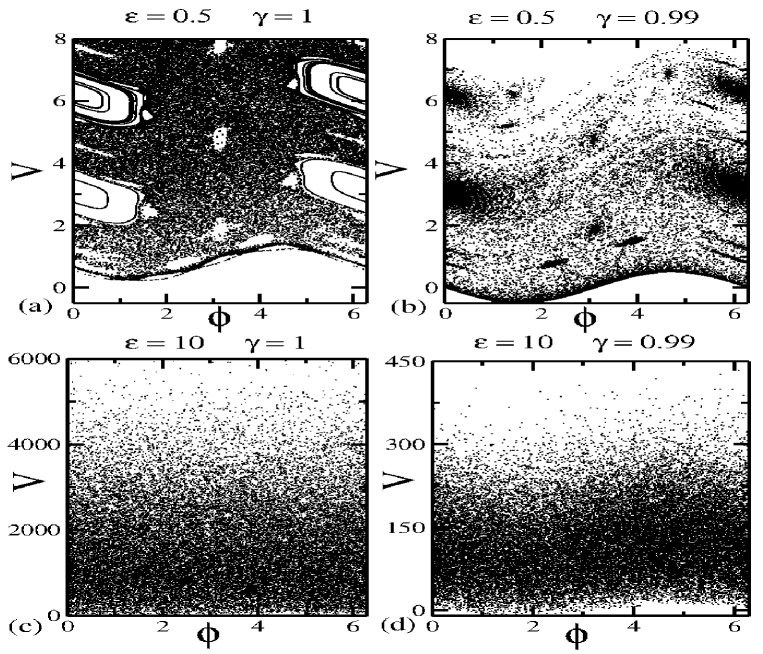
Figure 1: Snapshots of $(V,\phi)$ for the impact system considering either non-dissipative and dissipative dynamics. The control parameters used were: (a) $\epsilon=0.5$ and $\gamma=1$; (b) $\epsilon=0.5$ and $\gamma=0.99$; (c) $\epsilon=10$ and $\gamma=1$; and (d) $\epsilon=10$ and $\gamma=0.99$.

Figure 1 shows the phase space considering both non-dissipative and dissipative dynamics for the complete model. We used $100$ different initial conditions iterated up to $10^{4}$ collisions. Figure 1(a) shows the phase space for $\gamma=1$ and $\epsilon=0.5$. Easily observed and typical of Hamiltonian systems is the mixed dynamics scenario. It contains, indeed, stability islands and chaotic seas. Because of the absence of invariant tori – invariant spanning curves limiting the size of the chaotic sea – unlimited diffusion in velocity is observed. This phenomenon is known also as Fermi Acceleration (FA) ref36 can be slowed down by the presence of stickiness ref35 . In this case, a chaotic orbit may passes nearby a stability island and be trapped there around it for a finite time ref3 ; ref4 . Opposite to trapping, the so called accelerating modes, produced by resonances, can affect globally the dynamics ref37 leading to a fast acceleration.

Dissipation, introduced by inelastic collisions, however destroys the mixed structure of the phase space. As shown in Fig. 1(b) for $\gamma=0.99$ and $\epsilon=0.5$, the blurred points, suggesting a chaotic attractor, represent nothing more than transient orbits, which shall settle down at asymptotic fixed points (sinks) for a sufficiently long time. Figure 1(c) was constructed using $\epsilon=10$ and $\gamma=1$. The mixed structure is not observed at this scale and only chaotic orbits, diffusing unlimitedly are observed. Finally, Fig. 1(d) was obtained for $\epsilon=10$ and $\gamma=0.99$. The unlimited diffusion was replaced by a chaotic attractor, which has a limited range. This suppression was indeed expected since the determinant of the Jacobian matrix is written as

$${\rm Det}J=\gamma^{2}{{V_{n}+\epsilon\sin(\phi_{n})}\over{V_{n+1}+\epsilon\sin(\phi_{n+1})}}.$$ (5)

This result confirms that the introduction of dissipation can be considered as a powerful mechanism to suppress Fermi acceleration ref13 ; ref14 .

III Statistical and numerical results

Given the expressions of the mapping are already known, in this section, we describe the results obtained by numerical simulations. We focus particularly on the statistical analysis for the velocity of the particle. As it is already known ref14 ; ref15 ; ref16 , for large $\epsilon$ and in the presence of small dissipation, id est, $\epsilon>10$ and $\gamma>0.99$, the dynamics starting from either low or high velocity settles down at a stationary state for enough long time. The plateau of a saturation can be obtained from different ways: (i) imposing fixed point condition in the first equation of mappings (1) and (4), after averaging them in an ensemble of phase $\phi\in[0,2\pi]$; (ii) transforming the equation of the velocity in the discrete mapping into a differential equation and solve it using an ensemble of different initial phases $\theta\in[0,2\pi]$; (iii) doing numerical simulations and considering long time dynamics.

Because we have the dynamical equations of the mappings, different statistical investigations can be made using different types of averages. An observable which is immediate is the average velocity measured along the orbit. It is written as

$$V_{i}(n,\epsilon,\gamma)={1\over n}{\sum_{j=1}^{n}}V_{j}~{}.$$ (6)

We can use Eq. (6) and average it over an ensemble of different initial conditions, hence leading to

$$\langle{V}\rangle={1\over M}{\sum_{i=1}^{M}}V_{i}(n,\epsilon,\gamma)~{},$$ (7)

where $M$ represents an ensemble of initial conditions. For instance, the initial velocity is assumed constant and $M$ different phases uniformly distributed in the range $\phi\in[0,2\pi]$ are considered. The root mean square velocity is obtained as

$$V_{rms}=\sqrt{\langle{V^{2}}\rangle}~{}.$$ (8)

The procedure is the same as running Eqs. (6) and (7) but using $V^{2}$ rather than $V$. Finally, the deviation around the average velocity, $\omega$, see ref12 for instance, is obtained from

$$\omega=\sqrt{\langle V^{2}\rangle-{\langle V\rangle}^{2}}~{}.$$ (9)

As it is known, for large $\epsilon$, unlimited diffusion in velocity can be observed. Because of the dissipation, the unlimited diffusion is not allowed anymore. The average dynamics, no mater the initial velocity, will converge to an asymptotic state for large time. If the initial condition is large, the velocity of the particle decreases until reaches the stationary state. It is known in the literature for a similar system, that the decay of velocity is given by an exponential function danila1 ; danila2 and the speed of the decay depends on the strength of the dissipation. Stronger the dissipation, faster the decay.

In opposite way, starting with a small initial velocity, the dynamics leads the average velocity to experience an initial growth as a function of the number of collisions of the type $[\epsilon^{2}n]^{\beta}$. The acceleration exponent is $\beta=1/2$, similar to random walk systems, and eventually, the growing regime is replaced by a constant plateau. The crossover that marks the change from growth to the saturation is described by a power law on $(1-\gamma)^{z_{2}}$, with $z_{2}=-1$. The average velocity of the particle at the stationary regime depends either on the nonlinear parameter as well on the dissipation parameter as $\epsilon^{\alpha_{1}}(1-\gamma)^{\alpha_{2}}$ where $\alpha_{1}=1$ and $\alpha_{2}=-1/2$.

When the initial velocity is neither small or large, say below the saturation regime, an additional crossover time is observed in the curves leonel100 ; leonel101 . Such addition crossover is indeed produced by a break of symmetry of the probability distribution function for the velocity of the particle leading then to a bias and hence, producing a preferential direction of diffusion, yielding in a growth of the average velocity. Saturation is again observed for large enough time.

Based on the posed above, we show in Fig. 2, the behavior of $\langle V\rangle$ (black circles and squares), $V_{rms}$ (red up and down triangles) and $\omega$ (blue right and left triangles) as a function of the number of collisions $n$. The initial velocities were chosen in two different regimes: (i) high initial velocities $(V_{0}\approx 10^{3}\epsilon)$ and; (ii) low initial velocities $(V_{0}\approx\epsilon)$. We ensemble average the dynamics by considering the phase was equally distributed in the range $\phi\in[0,2\pi]$.

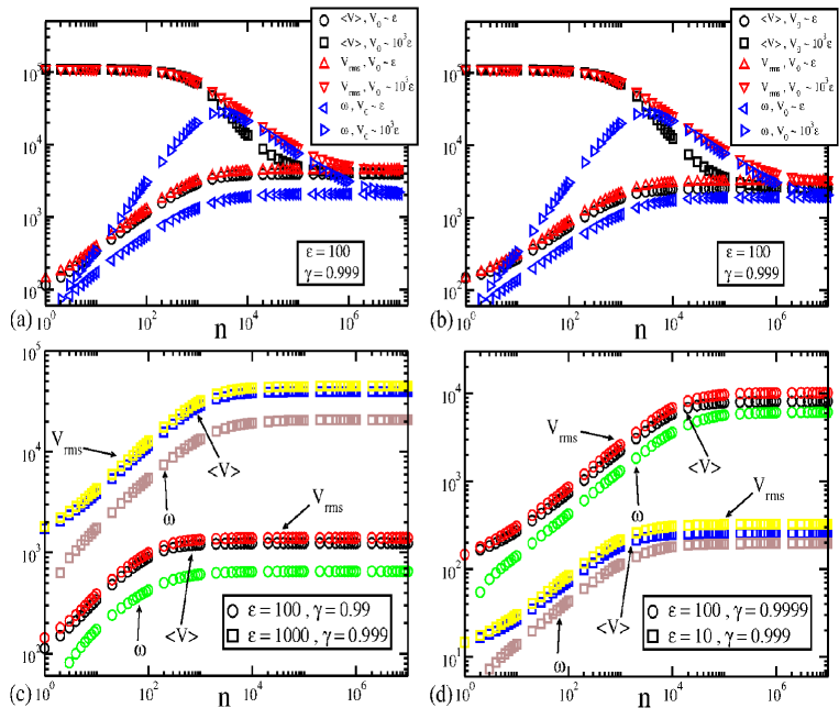
Figure 2: Evolution of $\langle V\rangle$, $V_{rms}$ and $\omega$ as function of $n$. The control parameters are shown in the figure. Complete in (a) and static wall approximation in (b) show the dynamics considering either small and large initial velocities. Small initial conditions are considered in (c) and (d), for the complete and static wall approximation. All curves show a converge to the stationary state for long times.

A comparison of the saturation of the three observables $\langle V\rangle$, $V_{rms}$ and $\omega$ is better seen in Figs. 2(c,d). Important to mention is that a change in the parameter $\epsilon$ leads to different saturation and it does not affect the crossover time. However, the parameter $\gamma$ changes both the saturation (stationary state) and the crossover times. With a scaling approach, as done previously in the literature, see for instance Refs. ref13 ; ref14 ; ref15 , a rescale can be done and overlap both curves, of the same observable, into an universal plot. However, in the scenario where high dissipation is considered, and we have low values for the parameter $\epsilon$, the scaling invariance is very difficult to be observed, since we have successive boundary crisis between manifolds and crisis between attractors crises .

As we will see in the next section, the numerical values of the saturation plateaus play an important role in the Thermodynamics analysis. The values of the plateaus for different values of the control parameters are shown in Tables 1 and 2. We see the saturation plateaus for the complete version are higher as compared to the static wall approximation. This is close connected to the probability distribution function of the velocity in the phase space. For short, the particle prefers to stay with high energy in the complete version while compared to the static wall approximation. Although the phase space is similar for both versions, their occupation are different.

$\epsilon$	$\gamma$	$\langle V\rangle$	$V_{rms}$	$\omega$
$10$	$0.999$	$257.54(5)$	$324.30(5)$	$197.09(2)$
$100$	$0.99$	$793.85(4)$	$995.03(5)$	$599.91(3)$
$100$	$0.999$	$2531.2(3)$	$3165.9(5)$	$1901.5(4)$
$100$	$0.9999$	$8091(9)$	$10079(9)$	$5999(9)$
$1000$	$0.999$	$25222(4)$	$31611(5)$	$19054(2)$

Table 1: Simplified mapping: Numerical values for the stationary state for $\langle V\rangle$, $V_{rms}$ and $\omega$ considering some pairs of ($\epsilon$,$\gamma$).

$\epsilon$	$\gamma$	$\langle V\rangle$	$V_{rms}$	$\omega$
$10$	$0.999$	$407.50(4)$	$461.23(4)$	$216.05(1)$
$100$	$0.99$	$1244.3(1)$	$1405.6(1)$	$653.53(3)$
$100$	$0.999$	$3959.7(2)$	$4469.0(3)$	$2071.7(2)$
$100$	$0.9999$	$12736(4)$	$14333(8)$	$6570(9)$
$1000$	$0.999$	$39608(1)$	$44694(2)$	$20706(1)$

Table 2: Complete mapping: Numerical values for the stationary state for $\langle V\rangle$, $V_{rms}$ and $\omega$ considering some pairs of ($\epsilon$,$\gamma$).

IV Thermodynamics and discussion

In this section we describe some thermodynamical results for the proposed models by an analytical method motivated by Ref. ref16 . We first present our results for the simplified version, see Eq. (4) and then, latter on, for the complete version, written in Eq. (1).

IV.1 Simplified version

To describe some of the thermodynamical properties for the simplified model, we used the equations of motion (4) considering many different trajectories. We then construct a histogram for the velocity variable, as an attempt to have an insight of the probability density function for the velocity.

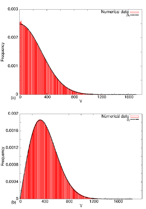
Figure 3: Histogram and probability distribution function for: (a) a simplified version, (b) complete version of the impact system.

From Fig. 3(a), we see that the histogram for the velocity has a half-Gaussian shape around zero. Such a shape allows us to write the probability density function for the velocity as a function of the type $\rho_{s}(V)=\frac{2}{\sqrt{2\pi}\sigma}e^{-\frac{V^{2}}{2\sigma^{2}}}$ for $V\in[0,\infty)$. Also, it can be shown numerically that the distribution probability for the phase variable is almost uniform and independent of the velocity variable and the averages can be taken separately from each other. Therefore, the mean squared velocity is given by

$$\langle{V^{2}}\rangle=\int_{0}^{\infty}V^{2}\rho_{s}(V)dV=\sigma^{2}.$$ (10)

It is known that for an ideal classical gas the temperature is proportional to the mean kinetic energy ref6 . Hence, we choose $T=\sigma^{2}$ and a straightforward integration yields

$$\langle{V}\rangle=\sqrt{\frac{2T}{\pi}}.$$ (11)

The expression for the temperature can also be obtained directly from the mapping (4). Squaring both sides of the expression for the velocity and taking the average over an ensemble of different initial phases $\phi\in[0,2\pi]$, we end up with

$$\langle V_{n+1}^{2}\rangle=\gamma^{2}\langle V_{n}^{2}\rangle_{V}+\frac{(1+\gamma)^{2}\epsilon^{2}}{2}.$$ (12)

Here the first term on the right side of the equation is averaged over the velocity probability distribution and the second term is obtained after averaging over the phase variable. At the stationary state, and considering the result of Eq.(10), we have $T=\gamma^{2}T+\frac{(1+\gamma)^{2}\epsilon^{2}}{2}$, thus yielding

$$T=\frac{(1+\gamma)\epsilon^{2}}{2(1-\gamma)}.$$ (13)

The other quantities can also be obtained by a similar procedure, as the one done in Eq.(10), in particular the root mean square velocity

$$\sqrt{\langle{V^{2}}\rangle}=\sqrt{T}~{},$$ (14)

and also the deviation around the mean velocity

$$\omega=\sqrt{\left(1-\frac{2}{\pi}\right)T}~{}.$$ (15)

Using Eq.(11), (14), (15) and the temperature given by equation (13) it is possible to recover the same numerical values for $\langle V\rangle$, $V_{rms}$ and $\omega$ shown in Table (1).

IV.2 Complete model

Let us now move on and discuss the results for the complete model. We proceed in a similar way as made to the simplified version. Figure 3(b) shows that the probability distribution of $V$ is not described anymore by a semi-Gaussian function. It can be approximated by a Weibull distribution weibull with a shape parameter $k=2$. The probability distribution function is then written as $\rho_{c}(V)=\frac{V}{T}e^{-\frac{V^{2}}{2T}}$, and we consider in our calculations that $V\in[0,\infty)$. In fairness, the real variation of velocity is $[-\epsilon,\infty)$ but the probability of finding a velocity in the interval $[-\epsilon,0)$ is very small as compared to the complementary range for the parameters considered in this paper. In this case, it can also be shown numerically, that the distribution probability for the phase variable is almost uniform and independent of the velocity variable. From such a distribution, we have

$$\langle{V}\rangle=\sqrt{\frac{\pi T}{2}}.$$ (16)

To discuss the temperature in terms of the dynamical equations, it turns convenient to rewrite the transcendental equation $F(\phi_{c})$ in a more convenient way as

$$\frac{1}{2}t^{2}-V_{n}t-m\epsilon\cos\left(\phi_{n}\right)+m\epsilon\cos\left(\phi_{n}+t\right)=0.$$ (17)

The parameter $m$ is defined in such a way that for $m=0$ the results for the simplified version are obtained. For $m=1$ we consider the complete version while for $0<m<1$ the solution for $t$ is required. Suppose $t$ can be approximated by

$$t = a_{0}+a_{1}m+a_{2}m^{2}+a_{3}m^{3}\ldots$$ (18)

for $0\leq m\leq 1$. Replacing Eq.(18) in the expression (17), after some straightforward algebra and rearranging properly the terms, we have

$$\begin{array}[]{llll}\left\{\frac{a_{0}^{2}}{2}-V_{n}a_{0}\right\}+[a_{0}a_{1}-V_{n}a_{1}-\epsilon\cos(\phi_{n}){}\\ +\epsilon\cos(\phi_{n}+a_{0})]m+[a_{0}a_{2}-V_{n}a_{2}{}\\ +\frac{a_{1}^{2}}{2}-\epsilon\sin(\phi_{n}+a_{0})a_{1}]m^{2}+[a_{0}a_{3}-V_{n}a_{3}{}\\ +a_{1}a_{2}-\epsilon\sin(\phi_{n}+a_{0})a_{2}-\frac{\epsilon\cos(\phi_{n}+a_{0})}{2}a_{1}^{2}]m^{3}=0.\end{array}$$ (19)

We truncate Eq.(19) at the third term and obtain the expressions for $a_{0}[V]$, $a_{1}[V,\phi]$, $a_{2}[V,\phi]$ and so on, considering that each element inside of the brackets must vanish. First analysis yields $a_{0}=2V$. Because the multiple collisions are rare as compared to the whole dynamics, solution of Eq. (17) is a good approximation to construct the probability. From numerical simulations we know that the probability of $V\leq\epsilon$ is small, then the series converges for $0\leq m<1$, hence $\frac{\left|a_{g}\right|}{\left|a_{g+1}\right|}<1$. The relations for $a_{0}[V]$, $a_{1}[V,\phi]$, $a_{2}[V,\phi]$ are

$$\left\{\begin{array}[]{llllll}a_{0}=2V_{n},{}\\ {}\\ a_{1}=\frac{\epsilon}{V_{n}}\left(\cos(\phi_{n})-\cos(\phi_{n}+2V_{n})\right),{}\\ {}\\ a_{2}=\frac{\epsilon^{2}}{V_{n}^{2}}\left\{\cos(\phi_{n})-\cos(\phi_{n}+2V_{n})\right\}{}\\ +\left\{\sin(\phi_{n}+2V_{n})-\frac{\cos(\phi_{n})-\cos(\phi_{n}+2V_{n})}{2V}\right\}.\end{array}\right.$$ (20)

Using Eq.(18) and the expressions given in (20), at the equilibrium state we have

$$\begin{array}[]{lll}\langle V_{n+1}\rangle=[\gamma\langle V_{n}\rangle-(1+\gamma)\epsilon\langle\sin(\phi_{n}+2V_{n})\rangle]{}\\ +[\gamma\langle a_{1}\rangle-(1+\gamma)\epsilon\langle\cos(\phi_{n}+2V_{n})a_{1}\rangle]m{}\\ +[\gamma\langle a_{2}\rangle-(1+\gamma)\epsilon\langle\cos(\phi_{n}+2V_{n})a_{2}-{}\\ \frac{\sin(\phi_{n}+2V_{n})}{2}a_{1}^{2}\rangle]m^{2}\end{array}$$ (21)

The terms $\left\langle\sin\left(\phi_{n}+2V_{n}\right)\right\rangle$ and $\left\langle a_{1}\right\rangle$ have zero value after averaging over the phase variable, which is distributed uniformly. Also, one can realize that $\left\langle\cos\left(\phi_{n}+2V_{n}\right)a_{1}\right\rangle=\langle\frac{\epsilon}{V_{n}}\cos(\phi_{n}+2V_{n})(\cos(\phi_{n})-\cos(\phi_{n}+2V_{n}))\rangle$. After take an average over the phase, one can obtain

$$\left\langle\cos\left(\phi_{n}+2V_{n}\right)a_{1}\right\rangle=\left\langle\frac{\epsilon}{V_{n}}\left(\frac{\cos\left(2V_{n}\right)}{2}-\frac{1}{2}\right)\right\rangle_{V}~{},$$ (22)

where the right-hand side term can be expressed by the cosine function expansion as

$$\left\langle\cos\left(\phi_{n}+2V_{n}\right)a_{1}\right\rangle=\epsilon\left\langle\sum_{l=0}^{\infty}\frac{\left(-1\right)^{l+1}\left(2V_{n}\right)^{2l+1}}{\Gamma\left(2l+3\right)}\right\rangle_{V}~{}.$$ (23)

The average over the coefficient $\left\langle a_{2}\right\rangle$ is obtained from $\langle a_{2}\rangle=\langle\frac{\epsilon^{2}}{V_{n}^{2}}(\cos(\phi_{n})-\cos(\phi_{n}+2V_{n}))(\sin(\phi_{n}+2V_{n})-\frac{\cos(\phi_{n})-\cos(\phi_{n}+2V_{n})}{2V_{n}})\rangle$. Considering then, an average over the phase one can obtain $\langle a_{2}\rangle=\langle\frac{\epsilon^{2}}{V_{n}^{2}}(\frac{\sin(2V_{n})}{2}-\frac{1}{2V_{n}}(1-\cos 2V_{n}))\rangle_{V}$, where now $\langle a_{2}\rangle$ is strictly written as function of the average over the velocity variable. One can expand this last expression for $\langle a_{2}\rangle$ in power series and obtain

$$\begin{array}[]{ll}\langle a_{2}\rangle=\langle\frac{\epsilon^{2}}{V_{n}^{2}}[V_{n}+\sum_{l=1}^{\infty}\frac{(-1)^{l}2V_{n})^{2l+1}}{2\Gamma(2l+2)}{}\\ -V_{n}-\sum_{l=1}^{\infty}\frac{(-1)^{l}(2V_{n})^{2l+1}}{\Gamma(2l+3)}]\rangle_{V},\end{array}$$ (24)

and after rearranging properly the terms, we have

$$\left\langle a_{2}\right\rangle=\epsilon^{2}\left\langle\sum_{l=0}^{\infty}\frac{\left(-1\right)^{l+1}2\left(2l+2\right)\left(2V_{n}\right)^{2l+1}}{\Gamma\left(2l+5\right)}\right\rangle_{V}~{}.$$ (25)

Finally, the average over the last term of Eq.(21) is given by

$$\left\langle\cos\left(\phi_{n}+2V_{n}\right)a_{2}-\frac{\sin\left(\phi_{n}+2V_{n}\right)}{2}a_{1}^{2}\right\rangle=0~{}.$$ (26)

For obtainment of Eq.(26), we considered that all third order trigonometric functions, like $\cos^{3}\left(\phi_{n}\right)$, and their crossed terms, like $\cos\left(\phi_{n}\right)\sin^{2}\left(\phi_{n}\right)$, have null averages over the phase variable.

With the previous results obtained in the expressions (23), (25) and (26), one may write Eq.(21) as

$$\begin{array}[]{lll}\left\langle V_{n+1}\right\rangle_{V}=\left\{\gamma\left\langle V_{n}\right\rangle_{V}\right\}+{}\\ \left\{-(1+\gamma)\epsilon^{2}\left\langle\sum_{l=0}^{\infty}\frac{\left(-1\right)^{l+1}\left(2V_{n}\right)^{2l+1}}{\Gamma\left(2l+3\right)}\right\rangle_{V}\right\}m{}\\ +\left\{\gamma\epsilon^{2}\left\langle\sum_{l=0}^{\infty}\frac{\left(-1\right)^{l+1}2\left(2l+2\right)\left(2V_{n}\right)^{2l+1}}{\Gamma\left(2l+5\right)}\right\rangle_{V}\right\}m^{2}\end{array}$$ (27)

Let us define an auxiliary term $\left\langle V^{2l}\right\rangle_{V}$, then

$$\left\langle V^{2l}\right\rangle_{V} = \int_{0}^{\infty}V^{2l}\frac{V}{T}e^{\frac{-V^{2}}{2T}}dV$$

if we call $u=\frac{V}{\sqrt{2T}}$, we have

$$\left\langle V^{2l}\right\rangle_{V} = \frac{(2T)^{l+1}}{2T}2\int_{0}^{\infty}u^{2(l+1)-1}e^{-u^{2}}du,$$

$$\left\langle V^{2l}\right\rangle_{V} = (2T)^{l}\Gamma\left(l+1\right)$$ (28)

where the $\Gamma$ function is well defined for $l>-1$ arfken .

Using Eq.(28) the expression of the average velocity, Eq. (27), can then be written as

$$\begin{array}[]{lll}\left\langle V_{n+1}\right\rangle_{V}=\left\{\gamma\left\langle V_{n}\right\rangle_{V}\right\}+{}\\ \left\{-(1+\gamma)\epsilon^{2}\sum_{l=0}^{\infty}\frac{\left(-1\right)^{l+1}2^{2l+1}\left(2T\right)^{l+1/2}\Gamma\left(l+3/2\right)}{\Gamma\left(2l+3\right)}\right\}m+{}\\ \left\{\gamma\epsilon^{2}\sum_{l=0}^{\infty}\frac{\left(-1\right)^{l+1}2\left(2l+2\right)2^{2l+1}\left(2T\right)^{l+1/2}\Gamma\left(l+3/2\right)}{\Gamma\left(2l+5\right)}\right\}m^{2},\end{array}$$ (29)

after rearranging properly the terms

$$\begin{array}[]{lll}\left\langle V_{n+1}\right\rangle_{V}=\gamma\left\langle V_{n}\right\rangle_{V}+{}\\ (1+\gamma)\epsilon^{2}\left(8T\right)^{1/2}\left\{\sum_{l=0}^{\infty}\frac{\left(-8T\right)^{l}\Gamma\left(l+3/2\right)}{\Gamma\left(2l+3\right)}\right\}m-{}\\ 2\gamma\epsilon^{2}\left(8T\right)^{1/2}\left\{\sum_{l=0}^{\infty}\frac{\left(2l+2\right)\left(-8T\right)^{l}\Gamma\left(l+3/2\right)}{\Gamma\left(2l+5\right)}\right\}m^{2}\end{array}$$ (30)

Recalling the following mathematical relation for the gamma function arfken .

$$\Gamma\left(2z\right) = \left(\pi\right)^{-\frac{1}{2}}2^{2z-1}\Gamma\left(z\right)\Gamma\left(z+\frac{1}{2}\right),$$ (31)

we may obtain after some straightforward algebra

$$\sum_{l=0}^{\infty}\frac{\left(-8T\right)^{l}\Gamma\left(l+3/2\right)}{\Gamma\left(2l+3\right)} = \frac{\sqrt{\pi}}{4}\sum_{l=0}^{\infty}\frac{\left(-2T\right)^{l}}{\Gamma\left(l+2\right)},$$ (32)

$$= \frac{\sqrt{\pi}}{8T}\left(1-e^{-2T}\right).$$

The last term of Eq. (30) stays as $\sum_{l=0}^{\infty}\frac{\left(2l+2\right)\left(-8T\right)^{l}\Gamma\left(l+3/2\right)}{\Gamma\left(2l+5\right)}=\frac{\sqrt{\pi}}{4}\sum_{l=0}^{\infty}\frac{\left(-2T\right)^{l}}{\left(l+2\right)\left(2l+3\right)\Gamma\left(l+1\right)}$. Again, rearranging the terms we have

$$\begin{array}[]{ll}\sum_{l=0}^{\infty}\frac{\left(2l+2\right)\left(-8T\right)^{l}\Gamma\left(l+3/2\right)}{\Gamma\left(2l+5\right)}={}\\ \frac{\sqrt{\pi}}{4}\sum_{l=0}^{\infty}\left[-\frac{\left(-2T\right)^{l}}{\left(l+2\right)\Gamma\left(l+1\right)}+\frac{\left(-2T\right)^{l}}{\left(l+3/2\right)\Gamma\left(l+1\right)}\right]\end{array}$$ (33)

Now we proceed to evaluate the sums in Eq.(33) with the following steps dingle : First we use the fact that $\frac{1}{n+1}=\int_{0}^{1}u^{n}du$, obtaining thus

$$\begin{array}[]{ll}\sum_{l=0}^{\infty}\frac{\left(2l+2\right)\left(-8T\right)^{l}\Gamma\left(l+3/2\right)}{\Gamma\left(2l+5\right)}={}\\ \frac{\sqrt{\pi}}{4}\sum_{l=0}^{\infty}\left[-\frac{\left(-2T\right)^{l}}{\Gamma\left(l+1\right)}\int_{0}^{1}u^{l+1}du+\frac{\left(-2T\right)^{l}}{\Gamma\left(l+1\right)}\int_{0}^{1}u^{l+\frac{1}{2}}du\right]~{},\end{array}$$ (34)

$$\begin{array}[]{ll}\sum_{l=0}^{\infty}\frac{\left(2l+2\right)\left(-8T\right)^{l}\Gamma\left(l+3/2\right)}{\Gamma\left(2l+5\right)}={}\\ \frac{\sqrt{\pi}}{4}\left[-\int_{0}^{1}e^{-2Tu}udu+\int_{0}^{1}e^{-2Tu}u^{\frac{1}{2}}du\right]~{},\end{array}$$ (35)

then we interchange the order of the summation and the integration. After that, we perform the sum over $l$, finally we integrate.

$$\begin{array}[]{ll}\sum_{l=0}^{\infty}\frac{\left(2l+2\right)\left(-8T\right)^{l}\Gamma\left(l+3/2\right)}{\Gamma\left(2l+5\right)}={}\\ \frac{\sqrt{\pi}}{4}\left[-\frac{1}{\left(2T\right)^{2}}+\frac{e^{-2T}}{\left(2T\right)^{2}}+\frac{\sqrt{\pi}}{2\left(2T\right)^{\frac{3}{2}}}erf\left(\sqrt{2T}\right)\right]~{},\end{array}$$ (36)

where $erf\left(x\right)=\frac{2}{\sqrt{\pi}}\intop_{0}^{x}e^{-x^{2}}dx$ is the error function and is in agreement with $\lim_{x\rightarrow\infty}erf\left(x\right)=1$. Therefore, for high temperatures, after replacing Eqs.(32) and (36) in Eq.(30), making $m=1$ and putting $\left\langle V\right\rangle$ in evidence we end up with

$$\left\langle V\right\rangle=\frac{1}{1-\gamma}\left[\frac{(1+\gamma)\epsilon^{2}}{2}\sqrt{\frac{\pi}{2T}}+\gamma\epsilon^{2}\frac{\pi}{\left(4T\right)}\right].$$ (37)

The first term on the right does indeed contributes at the limit of high temperatures, then, using Eq. (16) we find that

$$T=\frac{(1+\gamma)\epsilon^{2}}{2\left(1-\gamma\right)},$$ (38)

which is in remarkable well agreement with the result obtained for the simplified version of the model obtained in Eq. (13). Similar to discussed for the simplified version, we found also

$$\sqrt{\langle{V^{2}}\rangle}=\sqrt{2T}~{},$$ (39)

and the deviation around the average velocity

$$\omega=\sqrt{\left(2-\frac{\pi}{2}\right)T}~{}.$$ (40)

Using equations (16), (39), (40) and the temperature given by equation (38) it is possible to recover the same numerical values for $\langle V\rangle$, $V_{rms}$ and $\omega$ shown in Table (2).

IV.3 Discussion

Our findings shown in the previous sections were obtained from different approaches: (i) via numerical simulations; (ii) by the use direct average of the equation of the velocity; and (iii) by the probability distribution of the velocity. The agreement between these three approaches is remarkable. Let us now obtain a relation between $\langle{V}\rangle$, $\sqrt{\langle{V^{2}}\rangle}$, and $\omega$. For that we define new variables as $X=\ln(\langle{V}\rangle)$, $Y=\ln(\sqrt{\langle{V^{2}}\rangle})$, $Z=\ln(\omega)$. For the simplified version we obtain the following relations from Eqs. (11), (14) and (15)

$$Y=X+\frac{1}{2}\ln\left(\frac{\pi}{2}\right)~{},$$ (41)

$$Z=X+\frac{1}{2}\ln\left(\frac{\pi}{2}-1\right)~{},$$ (42)

$$Z=Y+\frac{1}{2}\ln\left(1-\frac{2}{\pi}\right)~{}.$$ (43)

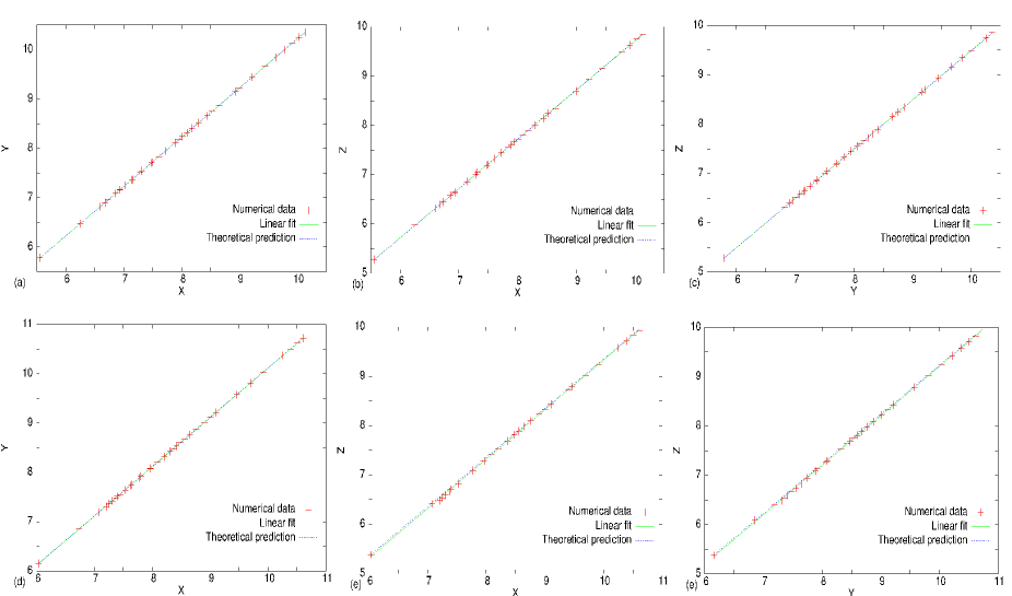
Figure 4: Plot of the observables obtained from numerical data, linear fit and theoretical prediction. Simplified version is shown in (a) for Eq. (41), (b) for Eq. (42), (c) for Eq. (43), while complete version is shown in (d) for Eq. (44), (e) for Eq. (45) and, (f) for Eq. (46).

For the complete version, the relations from Eqs. (16), (39) and (40) are

$$Y=X+\frac{1}{2}\ln\left(\frac{4}{\pi}\right)~{},$$ (44)

$$Z=X+\frac{1}{2}\ln\left(\frac{4}{\pi}-1\right)~{},$$ (45)

$$Z=Y+\frac{1}{2}\ln\left(1-\frac{\pi}{4}\right)~{}.$$ (46)

The behavior shown in Fig. 4, the comportment of equations (41-46) and numerical data regarding both the simplified and complete model, shows a remarkable agreement between the theory developed in this paper and the numerical results.

To illustrate better the novelty and results obtained in this paper we shown Table (3) which contains a comparison for the $\omega$ variable regarding analytical results, from Eqs.(15) and (13) for the simplified model (ASM), and Eqs.(40) and (38) for the complete model (ACM), with the numerical findings (NSM) and (NCM) respectively, shown in Tables (1) and (2). One can see that the agreement is quite good, which gives robustness to the theory developed in this study. Besides, it opens the possibility for the formalism to be extended to other similar dynamical systems, including billiard problems.

$\epsilon$	$\gamma$	$\omega_{ASM}$	$\omega_{NSM}$	$\omega_{ACM}$	$\omega_{NCM}$
$10$	$0.999$	$190.58$	$197.09(2)$	$207.12$	$216.05(1)$
$100$	$0.99$	$601.30$	$599.91(3)$	$653.50$	$653.53(3)$
$100$	$0.999$	$1905.8$	$1901.5(4)$	$2071.2$	$2071.7(2)$
$100$	$0.9999$	$6028$	$5999(9)$	$6551$	$6570(9)$
$1000$	$0.999$	$19058$	$19054(2)$	$20712$	$20706(1)$

Table 3: comparison for the $\omega$ variable regarding analytical results for the simplified model (ASM) and for the complete model (ACM), with the numerical findings for the simplified approach (NSM) and the complete one (NCM).

V Final Remarks and Conclusions

The dynamics of a dissipative impact system was described by nonlinear mappings for two different versions, complete and simplified, for the velocity of the particle and the phase of the vibrating wall. Dissipation was introduced via inelastic collisions leading the existence of attractors in the phase space.

A numerical and statistical investigation for the variables $\langle V\rangle$, $V_{rms}$ and $\omega$ (deviation of the average velocity) was made for both versions of the mappings. For long time series, these observables bend towards a saturation plateau which marks the stationary state. Such a regime varies as the control parameters associated with the dissipation $(\gamma)$ and ratio between acceleration $(\epsilon)$ are changed.

At the stationary state, the square velocity can be obtained. From equipartition theorem, such observable can be interpreted as an equilibrium temperature ref16 . We obtained analytical equations for the $\langle V\rangle$, $V_{rms}$ and $\omega$ variables in the equilibrium state as functions of the parameters of the model, with these equations we were able to calculate the numerical values of those variables without doing the simulations . A remarkable assembly was obtained considering both numerical and theoretical investigation, between statistical and thermal variables. This result gives robustness to the formalism, and opens ’new doors’ for similar analysis in other more complex dynamical systems, particularly in time dependent billiards.

References

- (1) R. C. Hilborn, Chaos and Nonlinear Dynamics: An Introduction for Scientists and Engineers. Oxford University Press, New York, 1994.
- (2) A. J. Lichtenberg, M.A. Lieberman, Regular and Chaotic Dynamics. Appl. Math. Sci. 38, Springer Verlag, New York, 1992.
- (3) G. M. Zaslasvsky, Physics of Chaos in Hamiltonian Systens, Imperial College Press, New York (2007).
- (4) G. M. Zaslasvsky, Hamiltonian Chaos and Fractional Dynamics, Oxford University Press, New York (2008).
- (5) N. Krylov, Works on the Foundations of Statistical Physics Princeton Univ. Press, Princeton, NJ, 1979.
- (6) R. K. Pathria, Statistical Mechanics, Elsevier – Burlington 2008.
- (7) F. H. Shu, F. C. Adams and S. Lizano, Annual review of astronomy and astrophysics, 25, 23, (1987).
- (8) Amir H. Safavi-Naeini, Jasper Chan, Jeff T. Hill, T. P. Mayer Alegre, Alex Krause and Oskar Painter, Phys. Rev. Lett., 108, 033602 (2012).
- (9) P. Dainese, P. St. J. Russell, N. Joly, J. C. Knight, G. S. Wiederhecker, H. L. Fragnito, V. Laude and A. Khelif, Nature Physics, 2, 388 (2006).
- (10) M. Zhang, G. S. Wiederhecker, S. Manipatruni, A. Barnard, P. McEuen, and M. Lipson, Phys Rev Lett, 109, 233906, (2012).
- (11) Gustavo S. Wiederhecker, Long Chen, Alexander Gondarenko and Michal Lipson, Nature, 462, 633, (2009).
- (12) A-L. Barabasi, H. E. Stanley, Fractal Concepts in Surface Growth.
- (13) E. D. Leonel and A. L. P. Livorati, Physica. A, 387, 1155, (2008).
- (14) A. L. P. Livorati, D. G. Ladeira and E. D. Leonel, Phys. Rev. E, 78, 056205, (2008).
- (15) J. -P. Eckmann and D. Ruelle, Rev. Mod. Phys. 57, 617 (1985).
- (16) E. D. Leonel, A. L. P. Livorati and A. M. Cespedes, Physica A, 404, 279, (2014).
- (17) E. D. Leonel and A. L. P. Livorati, Commun. Nonl. Sci. Num. Simul., 20, 159, (2015).
- (18) L. D. Pustilnikov, Theor. Math. Phys., 57, 1035, (1983).
- (19) P. J. Holmes, J. Sound and Vibration, 84, 173, (1982).
- (20) J. Guckenheimer and P. J. Holmes, Nonlinear Oscillations, Dynamical Systems, and Bifurcations of Vector Fields, Appl. Math. Sci. 42, Springer Verlag, New York, 1983.
- (21) R. M . Everson, Physica D, 19, 355, (1986).
- (22) J. M. Luck and A. Mehta, Phys. Rev. E, 48, 3988, (1993)
- (23) N. A. Burnham, A. J. Kulik, G. Gremaud and G. A. D. Briggs, Phys. Rev. Lett., 74, 5092, (1995).
- (24) P. Dainese, P. St. J. Russell, N. Joly, J. C. Knight, G. S. Wiederhecker, H. L. Fragnito, V. Laude and A. Khelif, Nature Physics, 2, 388 (2006).
- (25) M. Scheel, R. Seemann, M. Brinkmann, M. Di Michiel, A. Sheppard, B. Breidenbach and S. Herminghaus, Nat. Mater., 7, 189, (2008).
- (26) M. K. Müller, S. Ludinga and Thorsten Pöschel, Chem. Phys., 375, 600, (2010).
- (27) P. Müller, M. Heckel, A. Sack and T. Pöschel, Phys. Rev. Lett., 110, 254301, (2013).
- (28) F. Pacheco-Vazquez, F. Ludewig, and S. Dorbolo, Phys. Rev. Lett., 113, 118001, (2014).
- (29) D. Sternad, M. Duarte, H. Katsumata and S. Schaal, Phys. Rev. E, 63, 011902, (2000).
- (30) A. C. J. Luo and R. P. S. Han, Nonl. Dyn., 10, 1, (1996).
- (31) J. J. Barroso, M. V. Carneiro and E. E. N. Macau, Phys. Rev. E, 79, 026206, (2009).
- (32) A. Okniński and B. Radziszewski, Int. J. Nonl. Mech., 65, 226, (2014).
- (33) T. L. Vincent and A. I. Mees, Int. J. Bif. Chaos, 10, 579, (2000).
- (34) T. L. Vincent, Nonl. Dyn. Sys. Theo., 1 205, (2001).
- (35) A. L. P. Livorati, I. L. Caldas, C. P. Dettmann, and E. D. Leonel, Phys. Lett. A, 379, 2830, (2015).
- (36) A. L. P. Livorati, J. A. de Oliveira, D. G. Ladeira, and E. D. Leonel, Eur. Phys. J. Spec. Top., 223, 2953, (2014).
- (37) A. L. P. Livorati, T. Kroetz, C. P. Dettmann, I. L. Caldas and E. D. Leonel, Phys. Rev. E, 86, 036204, (2012).
- (38) A. K. Karlis, P. K. Papachristou, F. K. Diakonos, V. Constantoudis and P. Schmelcher, Phys. Rev. Lett., 97, 194102 (2006).
- (39) E. Fermi, Phys. Rev., 75, 1169, (1949).
- (40) T. Kroetz, A. L. P. Livorati, E. D. Leonel, and I. L. Caldas, Phys, Rev. E, 91, 012905, (2015).
- (41) D. F. Tavares, E. D. Leonel, R. N. Costa Filho, Physica A, 391, 5366 (2012).
- (42) D. F. Tavares, A. D. Araujo, E. D. Leonel, R. N. Costa Filho, Physica A, 392, 4231 (2013).
- (43) E. D. Leonel, J. Penalva, R. M. N. Teixeira, R. N. Costa Filho, M. R. Silva, J. A. de Oliveira, Phys. Lett. A 379, 1808 (2015).
- (44) D. F. M. Oliveira, M. R. Silva, E. D. Leonel, Phys. Lett. A 436, 909 (2015).
- (45) N. L. Johnson, S. Kotz, N. Balakrishnan, Continuous Univariate Distributions, Volume 1, Second Edition, Jonh Wiley and Sons (1995).
- (46) George B. Arfken Mathematical Methods for Physicists, Third Edition, Academic Press Inc. (1985).
- (47) R. B. Dingle Asymptotic Expansions: Their Derivation and Interpretation, Academic Press, (1973).