Black supernovae and black holes
in non-local gravity

Abstract

In a previous paper, we studied the interior solution of a collapsing body in a non-local theory of gravity super-renormalizable at the quantum level. We found that the classical singularity is replaced by a bounce, after which the body starts expanding. A black hole, strictly speaking, never forms. The gravitational collapse does not create an event horizon but only an apparent one for a finite time. In this paper, we solve the equations of motion assuming that the exterior solution is static. With such an assumption, we are able to reconstruct the solution in the whole spacetime, namely in both the exterior and interior regions. Now the gravitational collapse creates an event horizon in a finite comoving time, but the central singularity is approached in an infinite time. We argue that these black holes should be unstable, providing a link between the scenarios with and without black holes. Indeed, we find a non catastrophic ghost-instability of the metric in the exterior region. Interestingly, under certain conditions, the lifetime of our black holes exactly scales as the Hawking evaporation time.

1 Introduction

In Einstein gravity and under a set of physically reasonable assumptions, the complete gravitational collapse of a body creates a spacetime singularity and the final product is a black hole. The simplest example is the Oppenheimer-Snyder (OS) model, which describes the collapse of a homogeneous and spherically symmetric cloud of dust OS . However, it is often believed that the spacetime singularities created in a collapse are a symptom of the breakdown of the classical theory and they can be removed by quantum gravity effects. Alternatively, we can assume that spacetime singularities are resolved by employing a new action principle for classical gravity. However, the equations of motion of the new theory are typically quite difficult to solve. One can thus attempt to study toy-models, which can hopefully capture the fundamental features of the full theory. With a similar approach, one usually finds that the formation of a singularity is replaced by a bounce, after which the collapsing matter starts expanding frolov ; Frolov+-1 ; Frolov+ ; noi0 ; noi1 ; noi2 ; Tiberio ; rovelli ; torres ; torres2 ; garay ; Siegel ; koshe .

Even in simple models, it is usually quite difficult to find a global solution that covers the whole spacetime. Nevertheless, on the basis of general arguments, we can conclude that there are two plausible scenarios. One possibility is that the bounce generates a baby universe inside the black hole baby . This kind of scenario can generally be obtained analytically with a cut-and-paste technique, in which the singularity is removed and the spacetime is sewed to a new non-singular manifold describing an expanding baby universe. However, such a procedure seems to work only in very simple examples: the matching requires the continuity of the first and of the second fundamental forms across some hypersurface, which is not always possible because of the absence of a sufficient number of free parameters. In the second scenario, a black hole does not form. The gravitational collapse only creates a temporary trapped surface, which looks like an event horizon for a finite time (which may, however, be very long for a far-away observer). Such a possibility has recently attracted a lot of interest because of a paper by Hawking hawking , but actually it was proposed a long time ago by Frolov and Vilkovisky frolov ; Frolov+-1 , and was recently rediscovered by several groups Frolov+ ; noi0 ; noi1 ; noi2 ; Tiberio ; rovelli ; torres ; torres2 ; garay , following different approaches and within different models.

The aim of this paper is to go ahead in the investigation of this topic. Following Ref. torres , we start from a model for the exterior vacuum spacetime. We assume that the exterior metric is static, and we solve our effective equations of motion (EOM) for the non-local gravitational theory. With an ansatz for the interior solution, we are able to do the matching and eventually to obtain a solution for the whole spacetime. The result of this procedure is the formation of a black hole, characterized by a Cauchy internal horizon and an event horizon. More importantly, there is no bounce. The collapsing object approaches a singular state in an infinite time. It seems thus that the properties of the exterior solution, which could in principle be derived by the underlying fundamental theory, play a major role in the fate of the collapse. However, our exterior spacetime metric appears to be unstable because of the presence of a massive ghost. The latter can likely cause the destruction of the black hole, but the timescale is extremely long for a stellar-mass object. We thus argue that, once again, a true event horizon may never be created.

The content of the paper is as follows. In Section 2, we briefly review the gravitational collapse of a spherically symmetric cloud in classical general relativity. In Sections 3, we summarize the bouncing solutions (black supernovae) in weakly non-local theories of gravity found in noi0 ; noi2 . Moreover, we provide the correct spacetime structure missed in the previous papers. In Section 4, we follow the approach of Ref. torres and we construct the interior metric on the base of an external black hole metric hayward that captures all the features of the approximate solutions in non-local gravitational theories mmn . In Section 5, we provide a (in-)stability mechanism to reconcile the contradictory outcome of the previous sections. Indeed, the black hole metric shows a ghost instability which makes the black hole lifetime finite, but very long due to the non-locality scale. Summary and conclusions are reported in Section 6.

Throughout the paper, we use units in with $c=\hbar=1$, while we explicitly show Newton’s gravitational constant $G_{N}$.

2 Gravitational collapse in Einstein gravity

In the case of spherical symmetry, we can always write the line element in the comoving frame as

$$ds^{2}=-e^{2\nu}dt^{2}+\frac{R^{\prime 2}}{Y}dr^{2}+R^{2}d\Omega^{2}\;,$$ (1)

where $d\Omega^{2}$ represents the metric on the unit 2-sphere. The metric functions $\nu(r,t)$, $Y(r,t)$, and $R(r,t)$ must be determined by solving the Einstein equations for a given matter distribution. We note that $R(r,t)$ represents the collapsing areal coordinate, while the comoving radius $r$ is a coordinate “attached” to the collapsing fluid. The energy momentum tensor in comoving coordinates takes diagonal form and for a matter fluid source can be written as $T_{\mu}^{\nu}={\rm diag}\{-\rho,p_{r},p_{\theta},p_{\theta}\}$. With this set-up, the Einstein equations become

$$\rho = \frac{F^{\prime}}{4\pi R^{2}R^{\prime}}\;,$$ (2)

$$p_{r} = -\frac{\dot{F}}{4\pi R^{2}\dot{R}}\;,$$ (3)

$$\nu^{\prime} = 2\frac{p_{\theta}-p_{r}}{\rho+p_{r}}\frac{R^{\prime}}{R}-\frac{p_{r}^{\prime}}{\rho+p_{r}}\;,$$ (4)

$$\dot{Y} = 2\frac{\nu^{\prime}\dot{R}}{R^{\prime}}Y\;,$$ (5)

where ^′ indicates the derivative with respect to $r$, while $\dot{}$ the one with respect to $t$. The function $F$ is the Misner-Sharp mass of the system and is defined by (please note that there is a difference of a factor $2G_{N}$ in our definition of $F$ with respect our previous papers noi0 ; noi1 ; noi2 )

$$2G_{N}F=R(1-g_{\mu\nu}\nabla^{\mu}R\nabla^{\nu}R)\;.$$ (6)

It is easy to see that $F$ plays the same role as the mass parameter $M_{\rm s}$ in the Schwarzschild metric and represents the amount of gravitating matter within the shell $r$ at the time $t$ misner . Using the metric (1), $F$ can be written as

$$2G_{N}F=R\left(1-Y+e^{-2\nu}\dot{R}^{2}\right)\;.$$ (7)

We immediately see that these equations can be considerably simplified if the matter source satisfies $p_{r}=p_{\theta}$ and $p_{r}^{\prime}=0$. In this case, we have $\nu^{\prime}=0$, from which we get $\nu=\nu(t)$ and, by a suitable redefinition of the time gauge, we can set $\nu=0$. Eq. (5) becomes $\dot{Y}=0$, which can be integrated to give $Y=Y(r)=1+f(r)$. A cloud composed of non interacting particles has $p_{r}=p_{\theta}=0$ and satisfies the conditions above. This is the so called dust collapse and was first investigated in the case of a homogeneous density distribution in OS . From Eq. (3), we see that in the case of dust $F=F(r)$ and therefore the amount of matter enclosed within the shell $r$ is conserved. This means that there is no inflow or outflow of matter at any radius during the process of collapse. As a consequence, there is no flux of matter through the boundary of the star as well. Therefore, by setting the outer boundary of the cloud at the comoving radius $r=r_{b}$, which corresponds to the shrinking physical area-radius $R_{b}(t)=R(r_{b},t)$, we see that we can always perform the matching with an exterior Schwarzschild spacetime with mass parameter $M_{\rm s}=F(r_{b})$ matching .

Once we substitute $\nu$ and $Y$ for dust in the definition of the Misner-Sharp mass given by Eq. (7), we obtain the equation of motion for the system

$$\dot{R}=-\sqrt{\frac{2G_{N}F}{R}+f}\;.$$ (8)

The free function $f$ coming from the integration of Eq. (5) is related to the initial velocity of the infalling particles. If the cloud had no boundary and extended to infinity, then the velocity of particles at infinity would be given by $\lim_{r\rightarrow\infty}f(r)$. This allows us to distinguish three cases. Unbound collapse happens when particles have positive velocity at infinity. Marginally bound collapse happens when particles have zero velocity at infinity. Bound collapse happens when particles reach zero velocity at a finite radius.

There is a gauge degree of freedom given by setting the value of the area-radius $R$ at the initial time. This sets the initial scale of the system but does not affect the physics of the collapse. We can choose the initial scaling in such a way that at the initial time $t_{i}=0$ we have $R(r,0)=r$ and introduce a dimensionless scale factor $a(r,t)$ such that $R=ra$. Then the whole set of the Einstein equations can be rewritten in this gauge once we define two functions, $\mu(r)$ and $b(r)$, such that

$$F=r^{3}\mu\;,\quad f=r^{2}b\;.$$ (9)

The equation of motion (8) is immediately rewritten as

$$\dot{a}=-\sqrt{\frac{2G_{N}\mu}{a}+b}\;.$$ (10)

As a consequence of the above choice, we see that the regularity of the initial data at the center follows directly from the finiteness of $\mu$ and $b$. This choice makes also the appearance of the singularity more manifest, since the energy density becomes

$$\rho=\frac{3\mu+r\mu^{\prime}}{4\pi a^{2}(a+ra^{\prime})}\;,$$ (11)

which diverges for $a=0$ and is clearly finite at the initial time when $a=1$. As we can see, the homogeneous dust collapse model is obtained easily by setting $\mu$ and $b$ to be constant, namely $\mu=\mu_{0}$ and $b=b_{0}$. In this case, marginally bound collapse is simply given by $b_{0}=0$. Considering $\mu$ and/or $b$ as functions of $r$, one gets an inhomogeneous density profile, which corresponds to the so called Lemaìtre-Tolman-Bondi model (LTB) LTB . In both the homogeneous and inhomogeneous case, the collapse ends with the production of a gravitationally strong, shell-focusing singularity. The singularity is hidden behind the horizon in the OS model, while it may be visible to far-away observers in the LTB model dust .

3 Black supernovae

While most of the bouncing solutions are based on toy-models hawking ; noi1 ; rovelli ; torres ; torres2 ; garay , or at best on theories non renormalizable at the quantum level frolov , in Refs. noi0 ; noi2 we found the bounce in a family of asymptotically free weakly non-local theories of gravity. These theories are unitary, super-renormalizable or finite at the quantum level, and there are no extra degrees of freedom (ghosts or tachyons) expanding around the flat spacetime (for the details, see Refs. noi0 ; noi2 ). The simplest classical Lagrangian for these super-renormaliable theories reads kuzmin ; Krasnikov ; Tombo ; Khoury ; modesto ; modestoLeslaw ; universality ; Mtheory ; Dona

$$S_{g}=\frac{2}{\kappa^{2}}\int d^{4}x\sqrt{|g|}\Big{[}R+G_{\mu\nu}\frac{e^{{\rm H}(-\Box/\Lambda^{2})}-1}{\Box}R^{\mu\nu}\Big{]}\,,$$ (12)

where $G_{\mu\nu}$ is the Einstein tensor and $\kappa^{2}=32\pi G_{N}$. All the non-polynomiality is in the form factor $\exp{\rm H}(-\Box/\Lambda^{2})$, which must be an entire function. $\Lambda$ is the non-locality or quasi-polynomiality scale. The natural value of $\Lambda$ is of order the Planck mass and in this case all the observational constraints are satisfied. The theory is uniquely specified once the form factor is fixed, because the latter does not receive any renormalization: the ultraviolet theory is dominated by the bare action (that is, the counterterms are negligible). In this class of theories, we only have the graviton pole. Since $\exp{\rm H}(-\Box/\Lambda)$ is an entire function without zeros or poles in the whole complex plane, at perturbative level there are no ghosts and no tachyons independently of the number of time derivatives present in the action.

Let us now consider the gravitational collapse in the class of theories given by Eq. (12). In particular we look for approximate solutions for the interior of a collapsing body. The scale factor $a(t)$ is determined via the propagator approach frolov ; noi0 ; noi2 ; Calcagni:2013vra ; broda or the linearized equations of motion in the way we are going to describe. We consider a Friedman-Robertson-Walker (FRW) cosmological model since we can easily export the result to the gravitational collapse by inverting the time direction. We start writing the FRW metric as a flat Minkowski background plus a fluctuation $h_{\mu\nu}$,

$$g_{\mu\nu}=\eta_{\mu\nu}+\kappa\,h_{\mu\nu}\,,\quad ds^{2}=-dt^{2}+a(t)^{2}dx^{i}dx^{j}\delta_{ij}\,,$$ (13)

where $\eta_{\mu\nu}={\rm diag}(-1,1,1,1)$. The conformal scale factor $a(t)$ and the fluctuation $h_{\mu\nu}(t,\vec{x})$ are related by the following relations:

$$a^{2}(t)=1-\kappa h(t)\,,$$ (14)

$$h(t=t_{0})=0\,,$$

$$g_{\mu\nu}(t=t_{0})=\eta_{\mu\nu}\,,$$

$$h_{\mu\nu}(t,\vec{x})=-h(t)\,{\rm diag}(0,\delta_{ij})\equiv-h(t)\,\mathcal{I}_{\mu\nu}\,.$$ (15)

After a gauge transformation, we can rewrite the fluctuation in the usual harmonic gauge, in which the propagator is evaluated, namely

$$h_{\mu\nu}(x)\rightarrow h^{\prime}_{\mu\nu}(x)=h_{\mu\nu}(x)+\partial_{\mu}\xi_{\nu}+\partial_{\nu}\xi_{\mu}\,,$$

$$\xi_{\mu}(t)=\frac{3\kappa}{2}\,\left(\int_{0}^{t}h(t^{\prime})dt^{\prime},0,0,0\right)\,.$$ (16)

The fluctuation in the harmonic gauge reads

$$h^{\prime}_{\mu\nu}(t,\vec{x})=h(t)\,{\rm diag}(3,-\delta_{ij})\,,\,\,h^{\prime\,\mu}_{\mu}(t,\vec{x})=-6h(t).$$ (17)

We can then switch to the standard gravitational “barred” field $\bar{h}^{\prime}_{\mu\nu}$ defined by

$$\bar{h}^{\prime}_{\mu\nu}={h}^{\prime}_{\mu\nu}-\frac{1}{2}\eta_{\mu\nu}\,h^{\prime\,\lambda}_{\lambda}=2h(t)\,\mathcal{I}_{\mu\nu}\,,$$ (18)

satisfying $\partial^{\mu}\bar{h}^{\prime}_{\mu\nu}=0$. The Fourier transform of $\bar{h}^{\prime}_{\mu\nu}$ is

$$\tilde{\bar{h}}^{\prime}_{\mu\nu}(E,\vec{p})=2\tilde{h}(E)(2\pi)^{3}\delta^{3}(\vec{p})\,\mathcal{I}_{\mu\nu}\,.$$ (19)

For the generic case of a perfect fluid with equation of state $p=\omega\rho$, the scale factor for the homogeneous and spherically symmetric gravitational collapse (or cosmological metric) is (for $\omega\neq-1$)

$$a(t)=\left|\frac{t}{t_{0}}\right|^{\frac{2}{3(\omega+1)}}\,,$$ (20)

where now $t=0$ is the time of the formation of the singularity.

We can thus compute the Fourier transform $\tilde{h}(E)$ defined in (19). For $\omega\neq-1$, we have

$$\tilde{h}(E)=\frac{2\pi\delta(E)}{\kappa}+\frac{2\Gamma(\frac{4}{3(\omega+1)}+1)\mathrm{sin}(\frac{\pi}{2}\frac{4}{3(\omega+1)})}{\kappa t_{0}^{\frac{4}{3(\omega+1)}}\left|E\right|^{\frac{4}{3(\omega+1)}+1}}\,.$$ (21)

In the case of radiation and dust, we have

$$\tilde{h}(E) = \frac{2\pi\delta(E)}{\kappa}+\frac{2}{\kappa t_{0}E^{2}},\;\;\;\text{(radiation)}$$ (22)

$$\tilde{h}(E) = \frac{2\pi\delta(E)}{\kappa}+\frac{4\Gamma(\frac{4}{3})}{\sqrt{3}\kappa t_{0}^{4/3}\left|E\right|^{7/3}},\;\;\;\text{(dust)}\,.$$ (23)

Since the theory is asymptotically free, we can get a good approximation of the solution from the linear EOM of the non-local theory. In particular, given the energy tensor, we can extract the relation between the Einstein solution and the non-local solution comparing the following two equations,

$$\Box\bar{h}_{\mu\nu}^{\prime}=8\pi G_{N}T_{\mu\nu}\,,\qquad e^{H(\Box)}\Box\bar{h}_{\mu\nu}^{\prime\,\rm nl}=8\pi G_{N}T_{\mu\nu}\,,$$ (24)

where here $\bar{h}_{\mu\nu}^{\prime}$ is the solution of the linearized Einstein EOM, while $\bar{h}_{\mu\nu}^{\prime\,\rm nl}$ is the solution of the linearized non-local EOM. Therefore, the relation between the two gravitational perturbations is:

$$e^{H(\Box)}\,\bar{h}_{\mu\nu}^{\prime\,\rm nl}=\bar{h}_{\mu\nu}^{\prime}\,.$$ (25)

In Fourier transform, the above relation reads

$$\tilde{\bar{h}}^{\prime\,\rm nl}_{\mu\nu}(k)=e^{-H(k^{2})}\tilde{\bar{h}}_{\mu\nu}^{\prime}(k)\,,$$ (26)

or, for our homogeneous case,

$$\tilde{h}^{\rm nl}(E)=e^{-H(E^{2})}\tilde{h}(E)\,.$$ (27)

Considering the gravitational collapse for an homogeneous and spherically symmetric cloud and evaluating the anti-Fourier transform of (26), we find the solution for $h(t)$ and then the scale factor $a(t)$ (14). Everything in this section can be applied to the FRW cosmology as well as to the gravitational collapse. The solution for the gravitational collapse scenario is obtained by replacing $t$ with $-t+t_{0}$. For instance, in the radiation case and for the form factor $\exp(-\Box/\Lambda^{2})$, the result is noi0

$$a^{2}(t)=\frac{2e^{-\frac{1}{4}\Lambda^{2}(t-t_{0})^{2}}}{\Lambda\sqrt{\pi}\,t_{0}}+\frac{(t_{0}-t)\,\text{erf}\left(\frac{\Lambda(t_{0}-t)}{2}\right)}{t_{0}}\,,$$ (28)

where ${\rm erf}(z)=2\int_{0}^{z}\exp(-t^{2})dt/\sqrt{\pi}$. The classical singularity is now replaced by a bounce at $t=t_{0}$, after which the cloud starts expanding (hence the name black supernova). For dust, we find a very similar solution noi0 . The resulting profile for $a(t)$ is slightly different if we consider consistent form factor in Minkowski signature FrolovEven , namely $\exp(\Box^{N})$, where $N$ is an even integer. It is a general feature of these theories that the gravitational interaction is switched off at high energies, namely the theories are asymptotically free. In our framework, the asymptotic freedom is due to a higher derivative form factor, which makes gravity repulsive at very small distances. In terms of an effective picture in which gravity is supposed to be described by the Einstein-Hilbert theory and new physics is absorbed into the matter sector, the bounce comes from the conservation of the (effective) energy-momentum tensor: matter is transformed into a state with $\rho_{\rm eff}+p_{\rm eff}<0$, which is unstable and therefore the bounce is the only available possibility.

The bounce seems thus to be unavoidable in this class of theories. If we exclude the possibility of the creation of a baby universe, motivated by the problems mentioned in the introduction, a black hole, in the strict mathematical sense of the definition, never forms. Gravitational collapse only produces a trapped surface lasting for a finite time. No Cauchy and event horizon are formed. Since an apparent horizon cannot be destroyed from the inside, at least if we do not invoke exotic mechanisms like super-luminal motion, it must be destroyed from the outside. We thus argue that the solution outside the horizon cannot be static but must belong to the radiating Vaidya family. We can think of it as an effective negative energy flux destroying the horizon from the exterior. For a large black hole, we do not expect significant deviations from standard general relativity at the horizon (the value of scalar quantities like the Kretschmann invariant is much smaller than the Planck scale) and therefore the process is expected to be very slow. In other words, we recover the classical picture of an almost classical black hole and we can realize that the object is not a black hole only if the observation of a far-away observer lasts for a very long time.

In summary, with the approach employed in Ref. noi0 ; noi2 we start with a well-defined and consistent theory of gravity for the interior solution and we find that the bounce is unavoidable. On this basis, we can guess the exterior behavior. Fig. 1 shows the Finkelstein diagram of the collapse. Fig. 2 shows instead the corresponding Penrose diagram. We note that the latter corrects current diagrams presented in the literature. There is more likely only one trapped surface (not two), because gravity is switched off only inside the cloud of matter. The apparent horizon propagating inward from the cloud surface may either coincide with the cloud surface at the moment of the bounce (left panel in Fig. 1) or be in the exterior region (right panel). The actual situation may depend on the gravity theory. In our case we do not know because we are only able to solve the interior solution, so we cannot make predictions about the exterior region. The right panel in Fig. 1 may be motivated by the fact that the static black hole solutions in these theories have indeed an internal Cauchy horizon noi2 . For a finite observational time, the trapped surface first behaves as a black hole (left bottom side of the trapped surface in Fig. 2) and then as a while hole (left top side) rovelli .

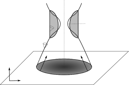
Figure 1: Finkelstein diagram of the black supernova scenario. The two panels differ for the position of the Cauchy horizon with respect to the boundary of the cloud. However, the spacetime structure of the gravitational collapse has a universal feature characterize by the formation of a trapped surface without any final black hole state.

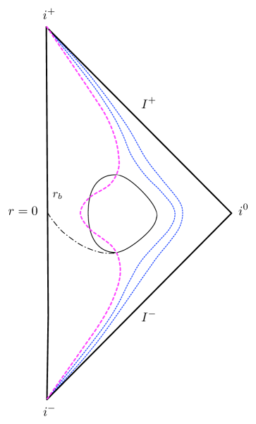
Figure 2: Penrose diagram of the black supernova scenario. There is a single trapped surface, which behaves for a finite time first as a black hole and then as a white hole. See the text for more details.

4 Black holes

In this section, we employ a semi-classical picture in which deviations from the classical theory are encoded in an effective Newton gravitational constant. $G_{N}$ is replaced by a function $G$ of the radial coordinate, which is used to reproduce the effects of (12) or a generic quantum effective action for gravity torres ; tavakoli . To this aim we start from the exterior solution and we reconstruct the interior.

4.1 Exterior solution

As done in torres ; torres2 , we assume that the exterior metric is a generalization of the classical Schwarzschild solution. The line element can be written as

$$ds^{2}=-\left(1-\frac{2G(x)M_{\rm s}}{x}\right)dt^{2}+\left(1-\frac{2G(x)M_{\rm s}}{x}\right)^{-1}dx^{2}+x^{2}d\Omega^{2}\;,$$ (29)

where $x$ is the radial coordinate in the exterior spacetime. In super-renormalizable/finite theories of gravity, spherically symmetric exact black hole solutions can be written in this form noi2 ; mmn . Notice the following key point: we are assuming that the exterior vacuum metric is static, as it is true in general relativity thanks to the Birkhoff theorem. A prototype of $G(x)$ that captures all the important and universal features in these theories has the following form

$$G(x)=\frac{x^{3}G_{N}}{x^{3}+L^{3}}\;,$$ (30)

where $L$ is a new scale and it is natural to expect it to be of order the Planck length, namely $L\approx L_{Pl}=G_{N}^{1/2}$. Of course, Eq. (29) is not a vacuum solution of the Einstein equations. If we impose the latter, we find an effective, or “unphysical”, matter source for the spacetime in the form of an energy-momentum tensor for a fluid with effective density and pressures given by

$$\rho^{\rm ext}=-p^{\rm ext}_{r}=\frac{M_{\rm s}G_{,x}}{4\pi G_{N}x^{2}}\;,\quad p^{\rm ext}_{\theta}=-\frac{M_{\rm s}G_{,xx}}{8\pi G_{N}x}\;.$$ (31)

New physics is encoded in $G(x)$, but one could have equivalently absorbed everything in a variable mass parameter $M(x)$, as done in noi2 ; mmn . In the next subsection, the line element in (29) will be matched to a suitable interior in the form of (1) through a 3-dimensional hypersurface $\Sigma$ describing the boundary of the collapsing cloud.

4.2 Interior solution

The use of a non-constant $G$ in the interior will affect the energy-momentum tensor by introducing some effective terms in the density and in the pressures. If $\Sigma$ is the comoving boundary hypersurface, then continuity of $g_{\theta\theta}$ and $g_{\phi\phi}$ implies that $R(r,t)|_{\Sigma}=R(r_{b},t)=x_{b}(\tau)$. We can then take the function $G(x)$ from the exterior and obtain the corresponding $G(R)$ in the interior through the matching conditions. Standard matching conditions imply continuity of the first and second fundamental forms across $\Sigma$ matching , namely the metric coefficients on the induced metric and the rate of change of the unit normal to $\Sigma$ must be the same on both sides. With the exterior metric given in Eq. (29), the matching conditions across $\Sigma$ imply that the density and the pressures in the interior take the form

$$\rho=\frac{G(R)F^{\prime}}{4\pi G_{N}R^{2}R^{\prime}}+\frac{FG_{,R}}{4\pi G_{N}R^{2}}\;,\quad p_{r}=-\frac{FG_{,R}}{4\pi G_{N}R^{2}}\;,\quad p_{\theta}=-\frac{FG_{,RR}}{8\pi G_{N}R}-\frac{F^{\prime}G_{,R}}{8\pi G_{N}RR^{\prime}}\;,$$ (32)

which reduce to the usual Einstein equations for dust in the case $G=G_{N}$ is constant. From these equations and Eq. (4), we find that $\nu^{\prime}=0$, and therefore the metric in the interior region still satisfies the same condition as the classical dust case. The line element can then be taken as

$$ds^{2}=-d\tau^{2}+\frac{R^{\prime}(r,\tau)^{2}}{1+f(r)}dr^{2}+R^{2}(r,\tau)d\Omega^{2}\;.$$ (33)

This is the usual LTB spacetime describing the collapse of a dust cloud, where now the energy-momentum tensor is the sum of the classical dust energy momentum-tensor and an effective contribution coming from the fact that $G$ is not constant. The equation of motion for the system becomes

$$\dot{R}^{2}=\frac{2G(R)F(r)}{R}+f(r)\;.$$ (34)

At this point, we have to specify the expression of $G(R)$ for the interior. As an example, for the sake of simplicity we consider a modified Hayward metric hayward that gives an equation (34) independent on the coordinate $r$, namely

$$G(R)=\frac{R^{3}G_{N}}{R^{3}+G_{N}F(r)L_{\rm Pl}^{2}}\;.$$ (35)

In the simplest case of a homogeneous cloud, $F(r)=\mu_{0}r^{3}$ with $\mu_{0}$ constant. Therefore

$$G(a)=\frac{a^{3}G_{N}}{a^{3}+G_{N}\mu_{0}L_{\rm Pl}^{2}}\,,$$ (36)

which is independent on the radial coordinate $r$. With the further assumption of marginally bound collapse, namely $f=0$, Eq. (34) becomes

$$\frac{\dot{a}^{2}}{a^{2}}=\frac{2G_{N}\mu_{0}}{a^{3}+G_{N}\mu_{0}L_{\rm Pl}^{2}}\;.$$ (37)

Eq. (37) can be integrate from $a$ to $1$, namely

$$\sqrt{2G_{N}\mu_{0}}\,t=\frac{2}{3}\left(-\sqrt{a^{3}+c}+\sqrt{c}\tanh^{-1}\left(\sqrt{\frac{a^{3}+c}{c}}\right)\right.\left.+\sqrt{c+1}-\sqrt{c}\tanh^{-1}\left(\sqrt{\frac{1}{c}+1}\right)\right)\,,$$ (38)

where $c=G_{N}\mu_{0}L_{\rm Pl}^{2}$. The classical solution can be recovered in the limit $c\rightarrow 0$

$$\sqrt{2G_{N}\mu_{0}}\,t=\frac{2}{3}\left(1-a^{3/2}\right).$$ (39)

The behavior of the scale factor is shown in Fig. 3 (solid line). The singular state $a=0$ is approached in an infinite time. For comparison, Fig. 3 also shows the case of general relativity (dashed line) whose analytic expression is given in (39). In the GR case $a=0$ is reached in a finite time. The Finkelstein diagram of this collapse is shown in Fig. 4. It is clear that in this scenario we have a real black hole with a Cauchy horizon and an event horizon.

Figure 3: Behavior of the scale factor $a(t)$ in the black hole scenario. The singular state with $a=0$ is approached in an infinite time. Therefore, a black hole forms presenting a Cauchy horizon and an event horizon.

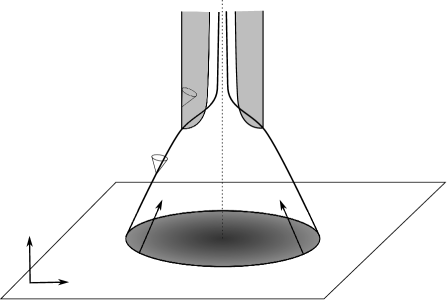
Figure 4: Finkelstein diagram of the black hole scenario. See the text for more details.

4.3 From in to out making use of the boundary conditions

The gravitational collapse and the cosmological solutions previously obtained in the asymptotic free limit of the weakly non-local theories are all consistent with a general effective FRW equation for the interior matter bouncing. This is a universal property of super-renormalizable asymptotically free gravitational theories including the recent proposed Lee-Wick gravities ShapiroComplex ; MeShapiro ; MeLW . The simplest effective FRW equation compatible with the general feature discussed in Section 3 reads

$$H^{2}=\frac{\dot{a}^{2}}{a^{2}}=\frac{8\pi G_{N}}{3}\left(1-\frac{\rho}{\rho_{c}}\right)\quad\,{\rm or}\quad\frac{\dot{a}^{2}}{2}=\frac{4\pi G_{N}}{3}\rho_{0}\left(\frac{a^{3}-a_{c}^{3}}{a^{3}}\right)\frac{1}{a}\;.$$ (40)

Here we only consider the homogeneous interior. Applying again the “Torres” procedure to reconstruct the metric in the vacuum from the metric in the matter region, we get the exterior spacetime imposing that the boundary conditions of the previous sections are satisfied. Comparing the interior FRW equation (40) with (34), we can derive the effective scaling of the Newton constant with the radial coordinate, namely

$$G(x)=\frac{x^{3}-l_{\Lambda}^{3}}{x^{3}}\,,$$ (41)

where $x$ is the radial coordinate. The exterior Schwarzschild spacetime is again (29). The metric is singular in $x=0$, but our derivation is correct only for $x\geqslant x_{\rm bounce}=l_{\Lambda}$, and $x_{\rm bounce}$ is a finite positive value. Therefore the metric (29) with (41) is only valid for $x\geqslant l_{\Lambda}$. The Cauchy and event horizons, if any, are located where the function $g_{00}(r)$ vanish. For different values of the mass $M$ we can have two roots, two coincident roots, or zero roots. Therefore, we here provide a justification for the diagrams in Section 3 that are only correct whether the metric in the external region present a Cauchy horizon. Nevertheless, this is the spacetime structure of any astrophysical object with $M\gg M_{\rm Pl}$ and then the metric in this subsection, by construction, is compatible with the internal matter bounce. For completion, the Kretschmann invariant is

$$R_{\mu\nu\rho\sigma}R^{\mu\nu\rho\sigma}=\frac{48G_{N}^{2}M^{2}\left(39l_{\Lambda}^{6}-10l_{\Lambda}^{3}r^{3}+r^{6}\right)}{r^{12}}\,.$$ (42)

5 Coexistence of the two scenarios and Hawking evaporation

The bouncing (black supernova) and the non-bouncing (singularity free black hole) solutions seem two different scenarios emerging from the same theory. In our class of weakly non-local gravities (12) and in many other frameworks frolov ; noi1 ; rovelli ; torres ; torres2 ; garay , the bounce appears to be unavoidable. However, we do not have the metric of the whole spacetime under control. If we make the reasonable assumption that the exterior vacuum solution is static, we end up with a regular black hole. The final product of the collapse would thus depend on whether we reconstruct the external spacetime (imposing the boundary conditions for the continuity of the metric and its first derivatives) from the approximate solution inside the matter (Section 3) or the matter interior spacetime from the static metric outside the collapsing body. While at the moment we cannot completely exclude the coexistence of both the dynamics, we would like to provide another possibility.

In this section we provide a mechanism to reconcile the two scenarios based on the stability analysis of the spacetime outside the matter region.

As we have already pointed out in Ref. noi2 , it is quite mysterious that in our class of weakly non-local theories of gravity (12) we can find the bouncing solution when we consider the gravitational collapse of a spherically symmetric cloud of matter and, on the other hand, regular black hole (approximate) solutions when we consider the static case. It is possible that all these regular black hole spacetimes are not stable and that their instability provides a link between the bouncing and non-bouncing scenarios.

The black hole solutions are indeed characterized by a de Sitter core, in which the effective cosmological constant is proportional to the mass of the collapsing object noi2 . From an analysis of the propagator, we can infer that there is a ghost-like pole, namely the spacetime is unstable. We can thus expect that the black hole decays into another black hole state with a de-Sitter core with a smaller effective cosmological constant in one or more steps through metastable configurations. The process should end when the effective cosmological constant is of the order of our non-local scale $\Lambda$, likely close to the Planck mass $M_{\rm Pl}$ if we identify the two scales in the theory. A solution with a de Sitter core proportional to $M_{\rm Pl}$ is not a black hole but a “particle” with a sub-Planck mass and without Cauchy and event horizons. Even if we do not know the intermedia states, the stability analysis may suggest that the black supernova and regular black hole scenarios are two faces of the same coin. In this way we also provide a reasonable justification for the well known instability of the Cauchy horizon. In our picture, the Cauchy horizon is just a sector of the close trapped surface, which of course do not extend to infinity. In all the approximate black hole solutions studied in the past noi2 ; mmn , three possible different spacetime structures were presented depending on the value of the mass: with two event horizons, with two coincident horizons (extremal black hole case), and without any event horizon (Planck mass particle). However, the correct way to interpret such spacetimes is not as unstable black hole because of the Cauchy horizon, but as different phases of the collapse and bounce (black supernova).

Let us now expand on the ghost-instability. While a spacetime with a ghost-instability compatible with the optical theorem in general does not exist at all Cline , because its decay time is not small but exactly zero, this is not true for weakly non-local theories vilenkin , and our class of theories (12) belongs to this group. It is crucial to notice that the singularity-free black hole metrics always show a de Sitter core with a huge effective cosmological constant, namely

$$\Lambda_{\rm eff}\approx MG_{N}\Lambda^{3}\,,$$ (43)

where $M$ is the mass of the body. Therefore, we can easily calculate the second variation of the action (12) for the tensor perturbations around the de Sitter spacetime, namely

$$g_{\mu\nu}=\bar{g}_{\mu\nu}+h_{\mu\nu}$$ (44)

where $\bar{g}_{\mu\nu}$ is the de Sitter metric. Here, we also use the parametrization

$$ds^{2}=-dt^{2}+\exp(2Ht)d\vec{x}^{2}\,,$$ (45)

where $8H^{2}=8\Lambda_{\rm eff}/3$. Moreover, the non-vanishing components for the tensor perturbations are purely spatial, $h^{0}_{\mu}$= 0, and satisfy the usual transverse and traceless conditions: $h^{i}_{i}=0$, $\partial_{i}h^{i}_{j}=0$. This computation was done for the first time in the paper khoury without introducing any cosmological constant in the action. The final result for the variation of the action reads

$$\delta S_{g}=2\kappa_{4}^{-2}\int d^{4}x\sqrt{|\bar{g}|}\,\frac{1}{4}h_{ij}[(\Box-8H^{2})+(\Box-2H^{2})\gamma(\Box)(\Box-2H^{2})]h^{ij},$$

$$\gamma(\Box)=\frac{e^{{\rm H}(-\Box/\Lambda^{2})}-1}{\Box}\,.$$ (46)

From the definition $\Box=-8H^{2}q^{2}=8H^{2}x$ (here we introduced a basis of eigenfunctions $h_{ij}^{(q)}$ for the $\Box$ operator, with dimensionless momentum eigenvalues $-q^{2}$), the inverse propagator is

$$\frac{P^{-1}(x)}{4H^{2}\kappa_{4}^{-2}}=x-1+\left(x-\frac{1}{4}\right)\frac{e^{{\rm H}(8H^{2}x/\Lambda^{2})}-1}{x}\left(x-\frac{1}{4}\right).$$ (47)

Notice that for the class of form factors we are considering here, ${\rm H}(z)={\rm H}(-z)$. If $\Lambda_{\rm eff}$ is large with respect to $\Lambda$, we find three poles, see Fig. 5. The second pole in the Fig. 5 corresponds to a ghost particle.

Figure 5: Plot of the inverse propagator (47) for $8H^{2}/\Lambda^{2}=1,10,25$. The lowest dashed curve corresponds to the local two derivative case, namely $\Lambda\rightarrow+\infty$ and $P^{-1}\propto x-1$. Here we used the following form factor: ${\rm H}(z)=\frac{1}{2}\left(\log\left(z^{4}\right)+\Gamma\left(0,z^{4}\right)+\gamma_{E}\right)$.

The outcome of this analysis is a ghost instability of the approximate black hole solution. However, in a non-local theory the instability is not catastrophic and can be estimated vilenkin ; Maggiore . Let us to consider the vacuum decay (in our case the black hole spacetime or actually the de Sitter spacetime) into a ghost particle and two normal gravitons khoury ; vilenkin ; Maggiore , ${\rm BH}\rightarrow g,h,h$. The decay probability per unit of volume and unit of time reads

$$\Gamma_{{\rm BH}\rightarrow g,h,h}=\frac{w}{VT}=\frac{\Lambda^{6}}{M_{\rm Pl}^{2}}e^{-{\rm H}(8H^{2}x_{0}/\Lambda^{2})}\,,$$ (48)

where $x_{0}$ is the ghost-like root in Fig. 5 and is obtained expanding the action near the ghost-pole. For the case of simplicity, here we assume $\Lambda=M_{\rm Pl}$. Therefore the lifetime is

$$\tau_{{\rm BH}\rightarrow g,h,h}=\frac{1}{\Gamma_{{\rm BH}\rightarrow g,h,h}V}=\frac{1}{VM_{\rm Pl}^{4}}e^{{\rm H}(8H^{2}x_{0}/\Lambda^{2})}\,.$$ (49)

The above decaying time is finite and actually very long because the effective cosmological constant is proportional to the mass of the black hole vilenkin , namley

$$\tau_{{\rm BH}\rightarrow g,h,h}=\frac{1}{VM_{\rm Pl}^{4}}e^{{\rm H}(8Mx_{0}/M_{\rm Pl})}\,.$$ (50)

If we consider an astrophysical object, $M$ is of order the Solar mass or more. The result is that the lifetime the all the processes of collapse, bounce and explosion take a very long time. The same exponential factor can be inferred from the ghost-instability presented in khoury , replacing the Lorentz-violating scale with the scale of non-locality in the theory (12).

We now explicitly consider a class of form factors compatible with super-renormalizability and asymptotic polynomiality, namely

$$e^{{\rm H}(z)}=e^{\frac{1}{2}\left(\gamma_{E}+\Gamma(0,z^{2(\gamma+1)})+\log z^{2(\gamma+1)}\right)},$$ (51)

whereby the decay time in the large mass limit simplifies to

$$\tau_{{\rm BH}\rightarrow g,h,h}\propto\frac{1}{VM_{\rm Pl}^{4}}\left(\frac{M}{M_{\rm Pl}}\right)^{\gamma+1}$$ (52)

Taking $V=1/M_{\rm Pl}$ and $\gamma=2$, we exactly reproduces the Hawking result

$$\tau_{{\rm BH}\rightarrow g,h,h}\propto\frac{1}{M_{\rm Pl}}\left(\frac{M}{M_{\rm Pl}}\right)^{3}\,.$$ (53)

It is quite impressive that the minimal super-renormalizable theory (the one for $\gamma=2$) embodies the Hawking evaporation process through the instability of the vacuum.

Summarizing this section, we have shown that in a large class of weakly non-local gravitational theories any (approximate) black hole solution presenting a de Sitter core near $r=0$ is unstable due to the presence of a ghost instability. However, in these theories this is not a catastrophe because of the non-locality scale. Therefore, the collapse of a cloud always produces a black supernova and never ends up with a black hole. Moreover, for the simplest range of theories compatible with super-renormalizability, the bouncing time perfectly agrees with the Hawking evaporation time. Despite this feature is not universal, it is impressive that it is a distinction of the minimal theory consistent at the quantum level.

6 Conclusions

In Ref. noi0 ; noi2 , we studied the gravitational collapse of a spherically symmetric cloud in a class of weakly non-local theories of gravity that are a field theory proposal for a consistent theory of quantum gravity kuzmin ; Tombo ; modesto ; modestoLeslaw . However, in noi0 ; noi2 we only derived an approximate solution for the interior, while the external spacetime was completely conjectured, as we were not able to find a metric for the whole spacetime. Nevertheless, we found a new picture for the gravitational collapse with the classical singularity replaced by a bounce, after which the collapsing body starts expanding. We inferred that black holes – in the mathematical sense of regions covered by an event horizon – do not form. The collapse only creates a temporary trapped surface, which can be interpreted as an event horizon only for a timescale shorter than the whole physical process. However, the latter might be extremely long for a stellar-mass object observed by a far-away observer. Our result is in agreement with those of other groups obtained with different approaches frolov ; Frolov+-1 ; Frolov+ ; rovelli ; torres ; torres2 ; garay .

In this paper, we have adopted a different approach to get an approximate solution for the whole spacetime. Following the idea in torres , we have started from the exterior region and assumed that the spacetime is static outside the matter. This is possible in classical general relativity as a consequence of the Birkhoff theorem, and it may be correct here as well. Such an assumption seems to play a crucial role in the final fate of the collapse.

The approximate vacuum solution has two universal features: the spacetime near $r=0$ is well approximated by the de Sitter metric and the global structure show up an event horizon as well as a Cauchy internal horizon. If the mass is comparable to the Planck mass, there are no horizons at all. It is clear that in a dynamical evolution of the black hole the Cauchy horizon instability is not a problem because it is just the internal part of o globally simply-connected trapped surface. These black holes are just like photo shoots of a non static but evolving black hole (where by evolution we mean the dynamics of the black hole mass).

After imposing the boundary conditions, we have reconstructed the interior matter metric that, in contrast to previous results reminded in the first part of the paper, does not show the expected bounce. On the contrary, there is an event horizon and a black hole does form. However, we have proved that the exterior metric is actually unstable due to the presence of a ghost-like pole in the propagator. The instability here is not catastrophic because of the non-locality scale that actually allowed us to estimate the lifetime of the system (49). It is quite remarkable that for the minimal super-renormalizable theory, the black hole lifetime is identical to the Hawking evaporation time (53).

- (1) J. R. Oppenheimer and H. Snyder, Phys. Rev. 56, 455 (1939).
- (2) V. P. Frolov and G. A. Vilkovisky, “Quantum Gravity Removes Classical Singularities And Shortens The Life Of Black Holes,” IC-79-69 (1979).
- (3) V. P. Frolov and G. A. Vilkovisky, Phys. Lett. B 106, 307 (1981).
- (4) V. P. Frolov, JHEP 1405, 049 (2014) [arXiv:1402.5446 [hep-th]]; V. P. Frolov, arXiv:1411.6981 [hep-th]; V. P. Frolov, A. Zelnikov and T. de Paula Netto, JHEP 1506, 107 (2015) [arXiv:1504.00412 [hep-th]]; V. P. Frolov, Phys. Rev. Lett. 115, 051102 (2015) [arXiv:1505.00492 [hep-th]].
- (5) C. Bambi, D. Malafarina and L. Modesto, Eur. Phys. J. C 74, 2767 (2014) [arXiv:1306.1668 [gr-qc]].
- (6) C. Bambi, D. Malafarina and L. Modesto, Phys. Rev. D 88, 044009 (2013) [arXiv:1305.4790 [gr-qc]]; C. Bambi, D. Malafarina, A. Marciano and L. Modesto, Phys. Lett. B 734, 27 (2014) [arXiv:1402.5719 [gr-qc]]; Y. Liu, D. Malafarina, L. Modesto and C. Bambi, Phys. Rev. D 90, 044040 (2014) [arXiv:1405.7249 [gr-qc]].
- (7) Y. Zhang, Y. Zhu, L. Modesto and C. Bambi, Eur. Phys. J. C 75, 96 (2015) [arXiv:1404.4770 [gr-qc]].
- (8) L. Modesto, T. de Paula Netto and I. L. Shapiro, JHEP 1504, 098 (2015) [arXiv:1412.0740 [hep-th]].
- (9) H. M. Haggard and C. Rovelli, Phys. Rev. D 92, 104020 (2015) [arXiv:1407.0989 [gr-qc]].
- (10) R. Torres, Phys. Lett. B 733, 21 (2014) [arXiv:1404.7655 [gr-qc]].
- (11) R. Torres and F. Fayos, Phys. Lett. B 733, 169 (2014) [arXiv:1405.7922 [gr-qc]].
- (12) C. Barcelo, R. Carballo-Rubio, L. J. Garay and G. Jannes, Class. Quant. Grav. 32, 035012 (2015) [arXiv:1409.1501 [gr-qc]].
- (13) T. Biswas, A. Mazumdar and W. Siegel, JCAP 0603, 009 (2006) [hep-th/0508194].
- (14) A. S. Koshelev, Class. Quant. Grav. 30, 155001 (2013) [arXiv:1302.2140 [astro-ph.CO]]; A. S. Koshelev and S. Y. Vernov, Phys. Part. Nucl. 43, 666 (2012) [arXiv:1202.1289 [hep-th]]; A. S. Koshelev, Rom. J. Phys. 57, 894 (2012) [arXiv:1112.6410 [hep-th]]; S. Y. Vernov, Phys. Part. Nucl. 43 (2012) 694 [arXiv:1202.1172 [astro-ph.CO]]; A. S. Koshelev and S. Y. Vernov, arXiv:1406.5887 [gr-qc].
- (15) V. Frolov, M. Markov and V. Mukhanov, Phys. Lett. B 216 , 272 (1989).
- (16) S. W. Hawking, arXiv:1401.5761 [hep-th].
- (17) S. A. Hayward, Phys. Rev. Lett. 96, 031103 (2006) [gr-qc/0506126].
- (18) L. Modesto, J. W. Moffat and P. Nicolini, Phys. Lett. B 695, 397 (2011) [arXiv:1010.0680 [gr-qc]].
- (19) C. W. Misner and D. H. Sharp, Phys. Rev. 136, B571 (1964).
- (20) W. Israel, Nuovo Cimento B 44, 1 (1966); Nuovo Cimento B 48, 463 (1966); F. Fayos, X. Jaen, E. Llanta and J. M. M. Senovilla, Phys. Rev. D 45, 2732 (1992); F. Fayos, J. M. M. Senovilla and R. Torres, Phys. Rev. D 54, 4862 (1996): F. Fayos, M. Mercè-Prats, J. M. M. Senovilla, Class. Quantum Grav. 12, 2565 (1995); P. S. Joshi and I. H. Dwivedi, Class. Quant. Grav. 16, 41 (1999).
- (21) R. C. Tolman, Proc. Natl. Acad. Sci. USA, 20, 410 (1934); H. Bondi, Mon. Not. Astron. Soc., 107, 343 (1947); G. Lemaìtre, Ann. Soc. Sci. Bruxelles I, A 53, 51 (1933).
- (22) P. S. Joshi and I. H. Dwivedi, Commun. Math. Phys. 146, 333 (1992); B. Waugh and K. Lake, Phys. Rev. D 38, 1315 (1988); R. P. A. C. Newman, Class. Quantum Grav. 3, 527 (1986); D. Christodoulou, Commun. Math. Phys. 93, 171 (1984); D. M. Eardley and L. Smarr, Phys. Rev. D 19, 2239 (1979).
- (23) Y. V. Kuzmin, Sov. J. Nucl. Phys. 50, 1011 (1989) [Yad. Fiz. 50, 1630 (1989)].
- (24) N. V. Krasnikov, Theor. Math. Phys. 73, 1184 (1987) [Teor. Mat. Fiz. 73, 235 (1987)].
- (25) E. T. Tomboulis, hep-th/9702146v1; E. T. Tomboulis, Mod. Phys. Lett. A 30, 1540005 (2015).
- (26) J. Khoury, Phys. Rev. D 76, 123513 (2007) [hep-th/0612052].
- (27) L. Modesto, Phys. Rev. D 86, 044005 (2012) [arXiv:1107.2403 [hep-th]]; L. Modesto, Astron. Rev. 8.2 (2013) 4-33 [arXiv:1202.3151 [hep-th]]; L. Modesto, arXiv:1402.6795 [hep-th]; L. Modesto, arXiv:1202.0008 [hep-th].
- (28) L. Modesto and L. Rachwal, Nucl. Phys. B 889, 228 (2014) [arXiv:1407.8036 [hep-th]].
- (29) L. Modesto and L. Rachwal, Nucl. Phys. B 900, 147 (2015) [arXiv:1503.00261 [hep-th]]; L. Modesto, M. Piva and L. Rachwal, arXiv:1506.06227 [hep-th].
- (30) G. Calcagni and L. Modesto, Phys. Rev. D 91, 124059 (2015) [arXiv:1404.2137 [hep-th]].
- (31) P. Donà, S. Giaccari, L. Modesto, L. Rachwal and Y. Zhu, JHEP 1508, 038 (2015) [arXiv:1506.04589 [hep-th]].
- (32) G. Calcagni, L. Modesto and P. Nicolini, Eur. Phys. J. C 74, 2999 (2014) [arXiv:1306.5332 [gr-qc]].
- (33) M. J. Duff, Phys. Rev. D 9, 1837 (1974); B. Broda, Phys. Rev. Lett. 106, 101303 (2011) [arXiv:1011.6257 [gr-qc]].
- (34) V. P. Frolov and A. Zelnikov, arXiv:1603.00826 [hep-th].
- (35) Y. Tavakoli, J. Marto and A. Dapor, Int. J. Mod. Phys. D 23, 1450061 (2014) [arXiv:1303.6157 [gr-qc]].
- (36) I. L. Shapiro, Phys. Lett. B 744, 67 (2015) [arXiv:1502.00106 [hep-th]].
- (37) L. Modesto and I. L. Shapiro, Phys. Lett. B 755, 279 (2016) [arXiv:1512.07600 [hep-th]].
- (38) L. Modesto, arXiv:1602.02421 [hep-th].
- (39) J. M. Cline, S. Jeon and G. D. Moore, Phys. Rev. D 70, 043543 (2004) [hep-ph/0311312].
- (40) J. Garriga and A. Vilenkin, JCAP 1301, 036 (2013) [arXiv:1202.1239 [hep-th]].
- (41) J. Khoury, Phys. Rev. D 76, 123513 (2007) [hep-th/0612052].
- (42) M. Jaccard, M. Maggiore and E. Mitsou, Phys. Rev. D 88, 044033 (2013) [arXiv:1305.3034 [hep-th]].
- (43) Y. D. Li, L. Modesto and L. Rachwal, JHEP 1512, 173 (2015) [arXiv:1506.08619 [hep-th]].
- (44) F. Briscese and M. L. Pucheu, arXiv:1511.03578 [gr-qc].