Abstract

Extremes play a special role in Anomaly Detection. Beyond inference and simulation purposes, probabilistic tools borrowed from Extreme Value Theory (EVT), such as the angular measure, can also be used to design novel statistical learning methods for Anomaly Detection/ranking. This paper proposes a new algorithm based on multivariate EVT to learn how to rank observations in a high dimensional space with respect to their degree of ‘abnormality’. The procedure relies on an original dimension-reduction technique in the extreme domain that possibly produces a sparse representation of multivariate extremes and allows to gain insight into the dependence structure thereof, escaping the curse of dimensionality. The representation output by the unsupervised methodology we propose here can be combined with any Anomaly Detection technique tailored to non-extreme data. As it performs linearly with the dimension and almost linearly in the data (in $O(dn\log n)$), it fits to large scale problems. The approach in this paper is novel in that EVT has never been used in its multivariate version in the field of Anomaly Detection. Illustrative experimental results provide strong empirical evidence of the relevance of our approach.

1 Introduction

In an unsupervised framework, where the dataset consists of a large number of normal data with a smaller unknown number of anomalies, the ‘extreme’ observations are more likely to be anomalies than the others. In a supervised or semi-supervised framework, when a dataset made of observations known to be normal is available, the most extreme points delimit the outlying regions of the normal instances. In both cases, extreme data are often in a boundary region between normal and abnormal regions and deserve special treatment.

This angle has been intensively exploited in the one-dimensional setting ([17], [18], [5], [4], [13]), where measurements are considered as ‘abnormal’ when they are remote from central measures such as the mean or the median. Anomaly Detection (AD) then relies on tail analysis of the variable of interest and naturally involves Extreme Value Theory (EVT). Indeed, the latter builds parametric representations for the tail of univariate distributions. In contrast, to the best of our knowledge, multivariate EVT has not been the subject of much attention in the field of AD. Until now, the multivariate setup has been treated using univariate extreme value statistics, to be handled with univariate EVT. A simple explanation is that multivariate EVT models do not scale well with dimension: dimensionality creates difficulties for both model computation and assessment, jeopardizing machine-learning applications. In the present paper we fill this gap by proposing a statistical method which is able to learn a sparse ‘normal profile’ of multivariate extremes in relation with their (supposedly unknown) dependence structure, and, as such, may be employed as an extension of any AD algorithm.

Since extreme observations typically constitute few percents of the data, a classical AD algorithm would tend to classify them as abnormal: it is not worth the risk (in terms of ROC curve for instance) to try to be more precise in such low probability regions without adapted tools. Thus, new observations outside the observed support or close to its boundary (larger than the largest observations) are most often predicted as abnormal. However, in many applications (e.g. aircraft predictive maintenance), false positives (i.e. false alarms) are very expensive, so that increasing precision in the extremal regions is of major interest. In such a context, learning the structure of extremes allows to build a ‘normal profile’ to be confronted with new extremal data.

In a multivariate ‘Peaks-over-threshold’ setting, well-documented in the literature (see Chapter 9 in [1] and the references therein), one observes realizations of a $d$-dimensional r.v. $\mathbf{X}=(X_{1},...,X_{d})$ and wants to learn the conditional distribution of excesses, $\left[~{}\mathbf{X}~{}|~{}\|\mathbf{X}\|_{\infty}\geq\mathbf{u}~{}\right]$ with $\|\mathbf{X}\|_{\infty}=\max_{1\leq i\leq d}|X_{i}|$ (notice incidentally that the present analysis could be extended to any other norm on $\mathbb{R}^{d}$), above some large threshold $\mathbf{u}$. The dependence structure of such excesses is described via the distribution of the ‘directions’ formed by the most extreme observations - the so-called angular probability measure, which has no natural parametric representation, which makes inference more complex when $d$ is large. However, in a wide range of applications, one may expect the occurrence of two phenomena: 1- Only a ‘small’ number of groups of components may be concomitantly extreme (relatively to the total number of groups $2^{d}$). 2- Each of these groups contains a reduced number of coordinates (w.r.t.. the dimension $d$). The main purpose of this paper is to propose a method for the statistical recovery of such subsets, so as to reduce the dimension of the problem and thus to learn a sparse representation of extreme – not abnormal – observations. In the case where hypothesis 2- is not fulfilled, such a sparse ‘normal profile’ can still be learned, but it then looses the low dimensional property.

In an unsupervised setup - namely when data include unlabeled anomalies - one runs the risk of fitting the ‘normal profile’ on abnormal observations. It is therefore essential to control the complexity of the output, especially in a multivariate setting where EVT does not impose any parametric form to the dependence structure. The method developed in this paper hence involves a non-parametric but relatively coarse estimation scheme, which aims at identifying low dimensional subspaces supporting extreme data. As a consequence, this method is robust to outliers and also applies when the training dataset contains a (small) proportion of anomalies.

Most of classical AD algorithms provide more than a predictive label, abnormal vs. normal. They return a real valued function, inducing a preorder/ranking on the input space. Indeed, when confronted with massive data, being able to rank observations according to their supposed degree of abnormality may significantly improve operational processes and allow for a prioritization of actions to be taken, especially in situations where human expertise required to check each observation is time-consuming (e.g. fleet management). Choosing a threshold for the ranking function yields a decision function delimiting normal regions from abnormal ones. The algorithm proposed in this paper deals with this problem of anomaly ranking and provides a ranking function (also termed a scoring function) for extreme observations. This method is complementary to other AD algorithms in the sense that a standard AD scoring function may be learned using the ‘non extreme’ (below threshold) observations of a dataset, while ‘extreme’ (above threshold) data are used to learn an extreme scoring function. Experiments on classical AD datasets show a significant performance improvement in terms of precision-recall curve, while preserving undiluted ROC curves. As expected, the precision of the standard AD algorithm is improved in extremal regions, since the algorithm ‘takes the risk’ not to consider systematically as abnormal the extremal regions, and to adapt to the specific structure of extremes instead. These improvements may typically be useful in applications where the cost of false positives (i.e. false alarms) is very expensive.

The structure of the paper is as follows. The algorithm is presented in Section 2. In Section 3, the whys and wherefores of EVT connected to the present analysis are recalled before a rationale behind the estimation involved by the algorithm. Experiments on both simulated and real datasets are performed respectively in Section 4 and 5.

2 A dependence-based AD algorithm

The purpose of the algorithm presented below is to rank multivariate extreme observations, based on their dependence structure. The present section details the algorithm and provides the heuristic of the mechanism at work, which can be understood without knowledge of EVT. A theoretical justification which does rely on EVT is given in Section 3. The underlying assumption is that an observation is potentially abnormal if its ‘direction’ (after a standardization of each marginal) is special regarding to the other extreme observations. In other words, if it does not belong to the (sparse) support of extremes. Based on this intuition, a scoring function is built to compare the degree of abnormality of extreme observations.

Let $\mathbf{X}_{1},.\ldots,\mathbf{X}_{n}$ $\mathit{i.i.d.}$ random variables in $\mathbb{R}^{d}$ with joint (resp. marginal) distribution $F$ (resp. $F_{j}$, $j=1,\ldots,d$). Marginal standardization is a natural first step when studying the dependence structure in a multivariate setting. The choice of standard Pareto margins $V^{j}$ (with $\mathbb{P}(V^{j}>x)=1/x$, $x>0$) is convenient – this will become clear in Section 3. One classical way to standardize is the probability integral transform, $T:\mathbf{X}_{i}\mapsto\mathbf{V}_{i}=((1-F_{j}(X_{i}^{j}))^{-1})_{1\leq j\leq d}$, $i=1,\ldots,n$. Since the marginal distributions $F_{j}$ are unknown, we use their empirical counterpart $\hat{F}_{j}$, where $\hat{F}_{j}(x)=(1/n)\sum_{i=1}^{n}\mathds{1}_{X_{i}^{j}\leq x}$. Denote by $\hat{T}$ the rank transformation thus obtained and by $\hat{\mathbf{V}}_{i}=\hat{T}(\mathbf{X}_{i})$ the corresponding rank-transformed observations.

Now, the goal is to measure the ‘correlation’ within each subset of features $\alpha\subset\{1,...,d\}$ at extreme levels (each $\alpha$ corresponding to a sub-cone of the positive orthant), that is, the likelihood to observe a large $\mathbf{\hat{V}}$ which verifies the following condition: $\hat{V}^{j}$ is ‘large’ for all $j\in\alpha$, while the other $\hat{V}^{j}$’s ($j\notin\alpha$) are ‘small’. Formally, one may associate to each such $\alpha$ a coefficient reflecting the degree of dependence between the features $\alpha$ at extreme levels. In relation to Section 3, the appropriate way to give a meaning to ‘large’ (resp. ‘small’) among extremes is in ‘radial’ and ‘directional’ terms, that is, $\|\mathbf{\hat{V}}\|>r$ (for some high radial threshold $r$), and $\hat{V}^{j}/\|\mathbf{\hat{V}}\|>\epsilon$ (resp. $\leq\epsilon$) for some small directional tolerance parameter $\epsilon>0$. Note that $\mathbf{\hat{V}}/\|\mathbf{\hat{V}}\|$ has unit norm and can be viewed as the pseudo-angle of the transformed data $\mathbf{\hat{V}}$. Introduce the truncated $\epsilon$-cones (see Fig. 2):

$$~{}\mathcal{C}_{\alpha}^{\epsilon}~{}=~{} \big{\{}\mathbf{v}\geq 0,~{}\|\mathbf{v}\|_{\infty}\geq 1,~{}v_{i}>\epsilon\|\mathbf{v}\|_{\infty}~{}\text{ for }i\in\alpha,$$ (1)

$$~{}~{}~{}~{}~{}~{}~{}~{}~{}~{}~{}~{}~{}~{}~{}~{}~{}~{}~{}~{}~{}~{}~{}~{}~{}~{}~{}~{}~{}~{}~{}~{}~{}~{}v_{i}\leq\epsilon\|\mathbf{v}\|_{\infty}~{}\text{ for }i\notin\alpha~{}~{}\big{\}}~{},$$

which defines a partition of $\mathbb{R}_{+}^{d}\setminus[0,1]^{d}$ for each fixed $\epsilon\geq 0$. This leads to coefficients

$$\mu_{n}^{\alpha,\epsilon}=(n/k)\mathbb{\hat{P}}_{n}\left((n/k)\mathcal{C}_{\alpha}^{\epsilon}\right),$$ (2)

where $\mathbb{\hat{P}}_{n}(.)=(1/n)\sum_{i=1}^{n}\delta_{\hat{V}_{i}}(.)$ is the empirical probability distribution of the rank-transformed data and $k=k(n)\to\infty$ s.t. $k=o(n)$ as $n\to\infty$. The ratio $n/k$ plays the role of a large radial threshold $r$. From our standardization choice, counting points in $(n/k)\,\mathcal{C}_{\alpha}^{\epsilon}$ boils down to selecting, for each feature $j\leq d$, the ‘$k$ largest values’ $X_{i}^{j}$ over the $n$ observations, whence the normalizing factor $\frac{n}{k}$. In an Anomaly Detection framework, the degree of ‘abnormality’ of new observation $\mathbf{x}$ such that $\hat{T}(\mathbf{x})\in\mathcal{C}_{\alpha}^{\epsilon}$ should be related both to $\mu_{n}^{\alpha,\epsilon}$ and the uniform norm $\|\hat{T}(\mathbf{x})\|_{\infty}$ (angular and radial components). As a matter of fact, in the transformed space - namely the space of the $\hat{V}_{i}$’s - the asymptotic mass decreases as the inverse of the norm, see (10). Consider the ‘directional tail region’ induced by $\mathbf{x}$, $A_{\mathbf{x}}=\{\mathbf{y}:T(\mathbf{y})\in\mathcal{C}_{\alpha}^{\epsilon}\,,\;\|T(\mathbf{y})\|_{\infty}\geq\|T(\mathbf{x})\|_{\infty}\}$ where $\mathbf{x}\in\mathcal{C}_{\alpha}^{\epsilon}$. Then, if $\|T(\mathbf{x})\|_{\infty}$ is large enough, we shall see (as e.g. in (11)) that $\mathbb{P}(\mathbf{X}\in A_{\mathbf{x}})\simeq\|\hat{T}(\mathbf{x})\|_{\infty}^{-1}\mu_{n}^{\alpha,\epsilon}$. This yields the scoring function $s_{n}(\mathbf{x})$ (4), which is thus an empirical version of $\mathbb{P}(\mathbf{X}\in A_{\mathbf{x}})$: the smaller $s_{n}(\mathbf{x})$, the more abnormal the point $\mathbf{x}$ should be considered.

This heuristic yields the following algorithm, referred to as the Detecting Anomaly with Multivariate EXtremes algorithm (DAMEX in abbreviated form). The complexity is in $O(dn\log n+dn)=O(dn\log n)$, where the first term on the left-hand-side comes from computing the $\hat{F}_{j}(X_{i}^{j})$ (Step 1) by sorting the data (e.g. merge sort). The second one comes from Step 2.

Remark 1

(Interpretation of the Parameters) In view of (1) and (2), $n/k$ is the threshold beyond which the data are considered as extreme. A general heuristic in multivariate extremes is that $k$ is proportional to the number of data considered as extreme. $\epsilon$ is the tolerance parameter w.r.t.. the non-asymptotic nature of data. The smaller $k$, the smaller $\epsilon$ shall be chosen.

Remark 2

(Choice of Parameters) There is no simple manner to choose the parameters $(\epsilon,~{}k,~{}\mu_{\min})$, as there is no simple way to determine how fast is the convergence to the (asymptotic) extreme behavior –namely how far in the tail appears the asymptotic dependence structure. In a supervised or semi-supervised framework (or if a small labeled dataset is available) these three parameters should be chosen by cross-validation. In the unsupervised situation, a classical heuristic ([6]) is to choose $(k,\epsilon)$ in a stability region of the algorithm’s output: the largest $k$ (resp. the larger $\epsilon$) such that when decreased, the dependence structure remains stable. Here, ‘stable’ means that the sub-cones with positive mass do not change much when the parameter varies in such region. This amounts to selecting the maximal number of data to be extreme, constrained to observing the stability induced by the asymptotic behavior. Alternatively, cross-validation can still be used in the unsupervised framework, considering one-class criteria such as the Mass-Volume curve or the Excess-Mass curve ([10, 3]), which play the same role as the ROC curve when no label is available. As estimating such criteria involve some volume estimation, a stepwise approximation (on hypercubes, whose volume is known) of the scoring function should be used in large dimension.

Remark 3

(Dimension Reduction) If the extreme dependence structure is low dimensional, namely concentrated on low dimensional cones $\mathcal{C}_{\alpha}$ – or in other terms if only a limited number of margins can be large together – then most of the $\hat{V}_{i}$’s will be concentrated on $\mathcal{C}_{\alpha}^{\epsilon}$’s such that $|\alpha|$ (the dimension of the cone $\mathcal{C}_{\alpha}$) is small; then the representation of the dependence structure in (3) is both sparse and low dimensional.

Algorithm 1

(DAMEX)
Input: parameters $\epsilon>0$,   $k=k(n)$,   $\mu_{\min}\geq 0$. 1. Standardize via marginal rank-transformation: $\hat{V}_{i}:=\big{(}1/(1-\hat{F}_{j}(X_{i}^{j}))\big{)}_{j=1,\ldots,d}$ . 2. Assign to each $\hat{V}_{i}$ the cone $\mathcal{C}_{\alpha}^{\epsilon}$ it belongs to. 3. Compute $\mu_{n}^{\alpha,\epsilon}$ from (2) $\rightarrow$ yields: (small number of) cones with non-zero mass 4. Set to $0$ the $\mu_{n}^{\alpha,\epsilon}$ below some small threshold $\mu_{\min}\geq 0$ to eliminate cones with negligible mass $\rightarrow$ yields: (sparse) representation of the dependence structure $\displaystyle(\mu_{n}^{\alpha,\epsilon})_{\alpha\subset\{1,\ldots,d\},\mu_{n}^{\alpha,\epsilon}>\mu_{\min}}$ (3) Output: Compute the scoring function given by $\displaystyle s_{n}(\mathbf{x}):=(1/\|\hat{T}(\mathbf{x})\|_{\infty})\sum_{\alpha}\mu_{n}^{\alpha,\epsilon}\mathds{1}_{\hat{T}(\mathbf{x})\in\mathcal{C}_{\alpha}^{\epsilon}}.$ (4)

The next section provides a theoretical ground for Algorithm 1. As shall be shown below, it amounts to learning the dependence structure of extremes (in particular, its support). The dependence parameter $\mu_{n}^{\alpha,\epsilon}$ actually coincides with a (voluntarily $\epsilon$-biased) natural estimator of $\mu(\mathcal{C}_{\alpha})$, where $\mu$ is a ‘true’ measure of the extremal dependence and $\mathcal{C}_{\alpha}$ is the truncated cone obtained with $\epsilon=0$ (Fig. 1),

$$\mathcal{C}_{\alpha}=\big{\{}\mathbf{x}\geq 0:~{}\|\mathbf{x}\|_{\infty}\geq 1,~{}x_{i}>0\text{ for }i\in\alpha,$$ (5)

$$~{}~{}~{}~{}~{}~{}~{}~{}~{}~{}~{}~{}~{}~{}~{}~{}~{}~{}~{}~{}~{}~{}~{}~{}~{}~{}~{}~{}~{}~{}~{}~{}~{}~{}~{}~{}~{}~{}~{}~{}~{}~{}~{}~{}~{}~{}x_{i}=0~{}\text{ for }i\notin\alpha~{}~{}~{}\big{\}}.$$

3 Theoretical framework

3.1 Probabilistic background

Univariate and multivariate EVT

Extreme Value Theory (EVT) develops models for learning the unusual rather than the usual. These models are widely used in fields involving risk management like finance, insurance, telecommunication or environmental sciences. One major application of EVT is to provide a reasonable assessment of the probability of occurrence of rare events. A useful setting to understand the use of EVT is that of risk monitoring. A typical quantity of interest in the univariate case is the $(1-p)^{th}$ quantile of the distribution $F$ of a random variable $X$, for a given exceedance probability $p$, that is $x_{p}=\inf\{x\in\mathbb{R},~{}\mathbb{P}(X>x)\leq p\}$. For moderate values of $p$, a natural empirical estimate is $x_{p,n}=\inf\{x\in\mathbb{R},~{}1/n\sum_{i=1}^{n}\mathds{1}_{X_{i}>x}\leq p\}$. However, if $p$ is very small, the finite sample $X_{1},\ldots,X_{n}$ contains insufficient information and $x_{p,n}$ becomes irrelevant. That is where EVT comes into play by providing parametric estimates of large quantiles: in this case, EVT essentially consists in modeling the distribution of the maxima (resp. the upper tail) as a Generalized Extreme Value (GEV) distribution, namely an element of the Gumbel, Fréchet or Weibull parametric families (resp. by a generalized Pareto distribution). Whereas statistical inference often involves sample means and the central limit theorem, EVT handles phenomena whose behavior is not ruled by an ‘averaging effect’. The focus is on large quantiles rather than the mean. The primal – and not too stringent – assumption is the existence of two sequences $\{a_{n},n\geq 1\}$ and $\{b_{n},n\geq 1\}$, the $a_{n}$’s being positive, and a non-degenerate cumulative distribution function (c.d.f.) $G$ such that

$$\lim_{n\to\infty}n~{}\mathbb{P}\left(\frac{X-b_{n}}{a_{n}}~{}\geq~{}x\right)=-\log G(x)$$ (6)

for all continuity points $x\in\mathbb{R}$ of $G$. If assumption (6) is fulfilled – it is the case for most textbook distributions – $F$ is said to be in the domain of attraction of $G$, denoted $F\in DA(G)$. The tail behavior of $F$ is then essentially characterized by $G$, which is proved to belong to the parametric family of GEV distributions, namely to be – up to rescaling – of the type $G(x)=\exp(-(1+\gamma x)^{-1/\gamma})$ for $1+\gamma x>0$, $\gamma\in\mathbb{R}$, setting by convention $(1+\gamma x)^{-1/\gamma}=e^{-x}$ for $\gamma=0$. The sign of $\gamma$ controls the shape of the tail and various estimators of the rescaling sequence as well as $\gamma$ have been studied in great detail, see e.g. [11], [19], [2].

The multivariate analogue of the assumption (6) concerns, again, the convergence of the tail probabilities, namely,

$$\lim_{n\to\infty}n~{}\mathbb{P}\left(\frac{X^{1}-b_{n}^{1}}{a_{n}^{1}}~{}\geq~{}x_{1}\;\text{~{}or~{}}\ldots\text{~{}or~{}}\;\frac{X^{d}-b_{n}^{d}}{a_{n}^{d}}~{}\geq~{}x_{d}\right)$$ (7)

$$~{}~{}~{}~{}~{}~{}~{}~{}~{}~{}~{}~{}~{}~{}~{}~{}~{}~{}~{}~{}~{}~{}~{}~{}~{}~{}~{}~{}~{}~{}~{}~{}~{}~{}~{}~{}~{}~{}~{}~{}~{}~{}~{}~{}~{}~{}~{}~{}~{}~{}~{}~{}~{}~{}~{}~{}~{}~{}~{}~{}~{}~{}~{}~{}~{}~{}=~{}-\log\mathbf{G}(\mathbf{x}),$$

(denoted $\mathbf{F}\in\textbf{DA}(\mathbf{G})$) for all continuity points $\mathbf{x}\in\mathbb{R}^{d}$ of $\mathbf{G}$. Here $a_{n}^{j}>0$ and $\mathbf{G}$ is a non degenerate multivariate c.d.f.. This implies that the margins $G_{1}(x_{1}),\ldots,G_{d}(x_{d})$ are univariate extreme value distributions, namely of the type $G_{j}(x)=\exp(-(1+\gamma_{j}x)^{-1/\gamma_{j}})$. Also, denoting by $F_{1},\ldots,F_{d}$ the marginal distributions of $\mathbf{F}$, assumption (7) implies marginal convergence, $F_{i}\in DA(G_{i})$ for $i=1,\ldots,n$. However, extending the theory and estimation methods from the univariate case is far from obvious, since the dependence structure of the joint distribution $\mathbf{G}$ comes into play and has no exact finite-dimensional parametrization.

Standardization and Angular measure

To understand the form of the limit $\mathbf{G}$ and dispose of the unknown sequences $(a_{n}^{j},b_{n}^{j})$, it is most convenient to work with marginally standardized variables, $V^{j}:=\frac{1}{1-F_{j}(X^{j})}$ and $\mathbf{V}=(V^{1},\ldots,V^{d})$, as introduced in Section 2. In fact (see [16], Proposition 5.10), the multivariate tail convergence assumption in (7) is equivalent to marginal convergences $F_{j}\in\text{DA}(G_{j})$ as in (6), together with regular variation of the tail of $\mathbf{V}$, i.e. there exists a limit measure $\mu$ on $\mathbf{E}=[0,\infty]^{d}\setminus\{0\}$, such that

$$n~{}\mathbb{P}\left(\frac{V^{1}}{n}~{}\geq~{}v_{1}\text{~{}or~{}}\cdots\text{~{}or~{}}\frac{V^{d}}{n}~{}\geq~{}v_{d}\right)\xrightarrow[n\to\infty]{}\mu[0,\mathbf{v}]^{c}$$ (8)

(where $[0,\mathbf{v}]=[0,v_{1}]\times\ldots\times[0,v_{d}]$). Thus, the variable $\mathbf{V}$ satisfies (7) with $\mathbf{a}_{n}=(n,\ldots,n)$, $\mathbf{b}_{n}=(0,\ldots,0)$. The so-called exponent measure $\mu$ has the homogeneity property: $\mu(t\,\cdot\,)=t^{-1}\mu(\,\cdot\,)$. To wit, $\mu$ is, up to a normalizing factor, the asymptotic distribution of $\mathbf{V}$ on extreme regions, that is, for large $t$ and any fixed region $A$ bounded away from $0$, we have

$$t\mathbb{P}(\mathbf{V}\in tA)\simeq\mu(A).$$ (9)

Notice that the limit joint c.d.f. $G$ can be retrieved from $\mu$ and the margins of $G$, via $-\log G(\mathbf{x})=\mu\left[\mathbf{0},\left(\frac{-1}{\log G_{1}(x_{1})},\dots,\frac{-1}{\log G_{d}(x_{d})}\right)\right]^{c}$. The choice of a marginal standardization to handle $V^{j}$’s variables is somewhat arbitrary and alternative standardizations lead to alternative limits.

Using the homogeneity property $\mu(t\,\cdot\,)=t^{-1}\mu(\,\cdot\,)$, it can be shown (see e.g. [7]) that in pseudo-polar coordinates, the radial and angular components of $\mu$ are independent: For $(v_{1},...,v_{d})\in\mathbf{E}$, let

$$R(\mathbf{v}):=\|\mathbf{v}\|_{\infty}~{}=~{}\max_{i=1}^{d}v_{i}$$

    and $$\Theta(\mathbf{v}):=\left(\frac{v_{1}}{R(\mathbf{v})},...,\frac{v_{d}}{R(\mathbf{v})}\right)\in S^{\infty}_{d-1}$$

where $S^{\infty}_{d-1}$ is the unit sphere in $\mathbb{R}^{d}$ for the infinity norm. Define the angular measure $\Phi$ (also called spectral measure) by $\Phi(B)=\mu(\{\mathbf{v}:R(\mathbf{v})>1,\Theta(\mathbf{v})\in B\})$, $B\in S^{\infty}_{d-1}$. Then, by homogeneity,

$$\mu(R>r,\Theta\in B)=r^{-1}\Phi(B)~{}.$$ (10)

In a nutshell, there is a one-to-one correspondence between $\mu$ and the angular measure $\Phi$, and any one of them can be used to characterize the asymptotic tail dependence of the distribution $F$.

Sparse support

For $\alpha$ a nonempty subset of $\{1,\ldots,d\}$ consider the truncated cones $\mathcal{C}_{\alpha}$ defined by Eq. (5) in the previous section and illustrated in Fig. 1. The family $\{\mathcal{C}_{\alpha},\alpha\subset\{1,\ldots,d\},\alpha\neq\emptyset\}$ defines a partition of $\mathbb{R}_{+}^{d}\setminus[0,1]^{d}$. In theory, $\mu$ may possibly allocate some mass on each cone $\mathcal{C}_{\alpha}$. A non-zero value of the cone’s mass $\mu(\mathcal{C}_{\alpha})$ indicates that it is not abnormal to record simultaneously large values of the coordinates $X^{j},j\in\alpha$, together with simultaneously small values of the complementary features $X^{j},j\notin\alpha$. On the contrary, zero mass on the cone $\mathcal{C}_{\alpha}$ (i.e. , $\mu_{\alpha}=0$) indicates that such records would be abnormal. A reasonable assumption in a lot of large dimensional use cases is that $\mu(\mathcal{C}_{\alpha})=0$ for the vast majority of the $2^{d}-1$ cones $\mathcal{C}_{\alpha}$, especially for large $|\alpha|$’s.

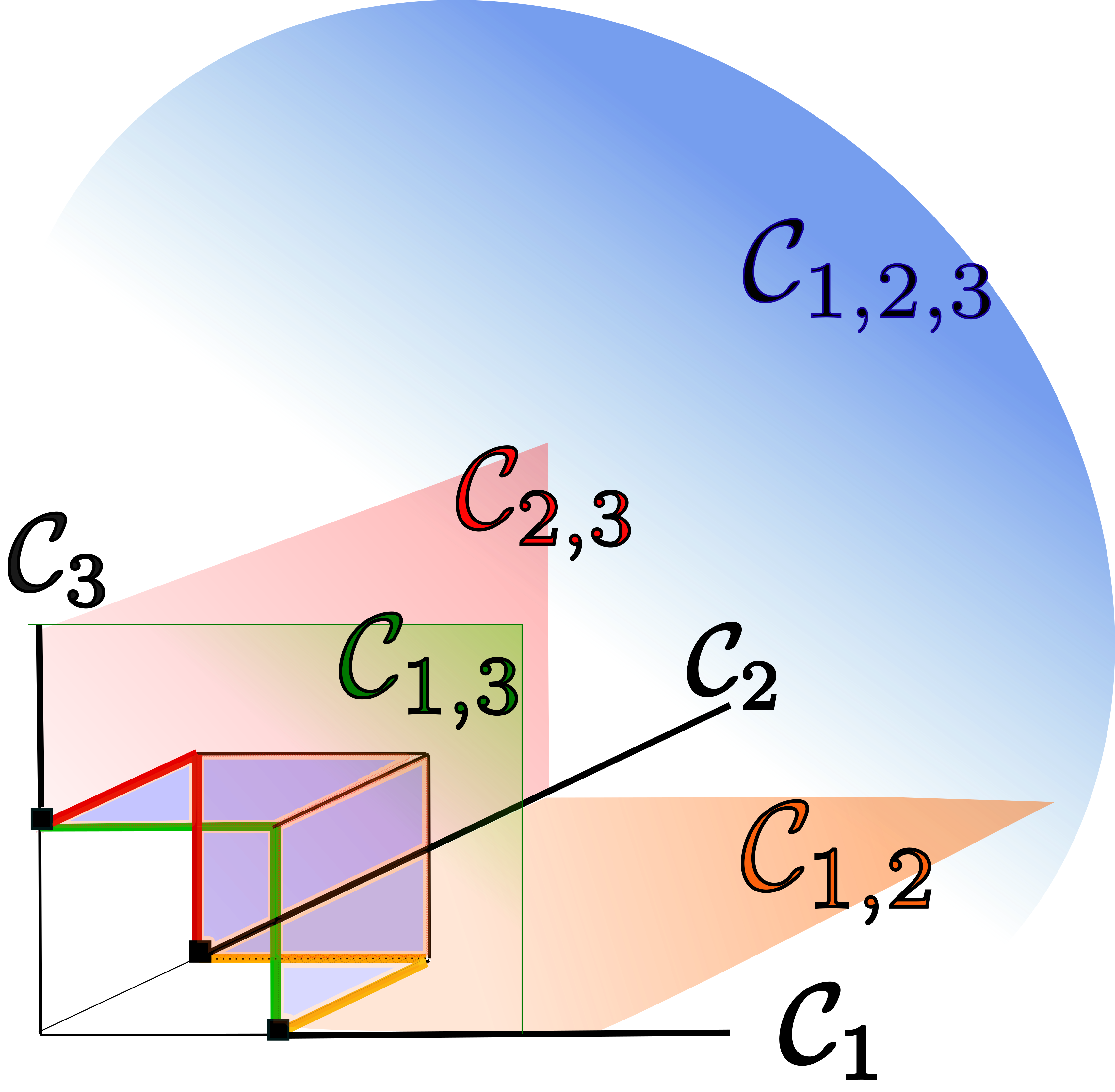
Figure 1: Truncated cones in 3D

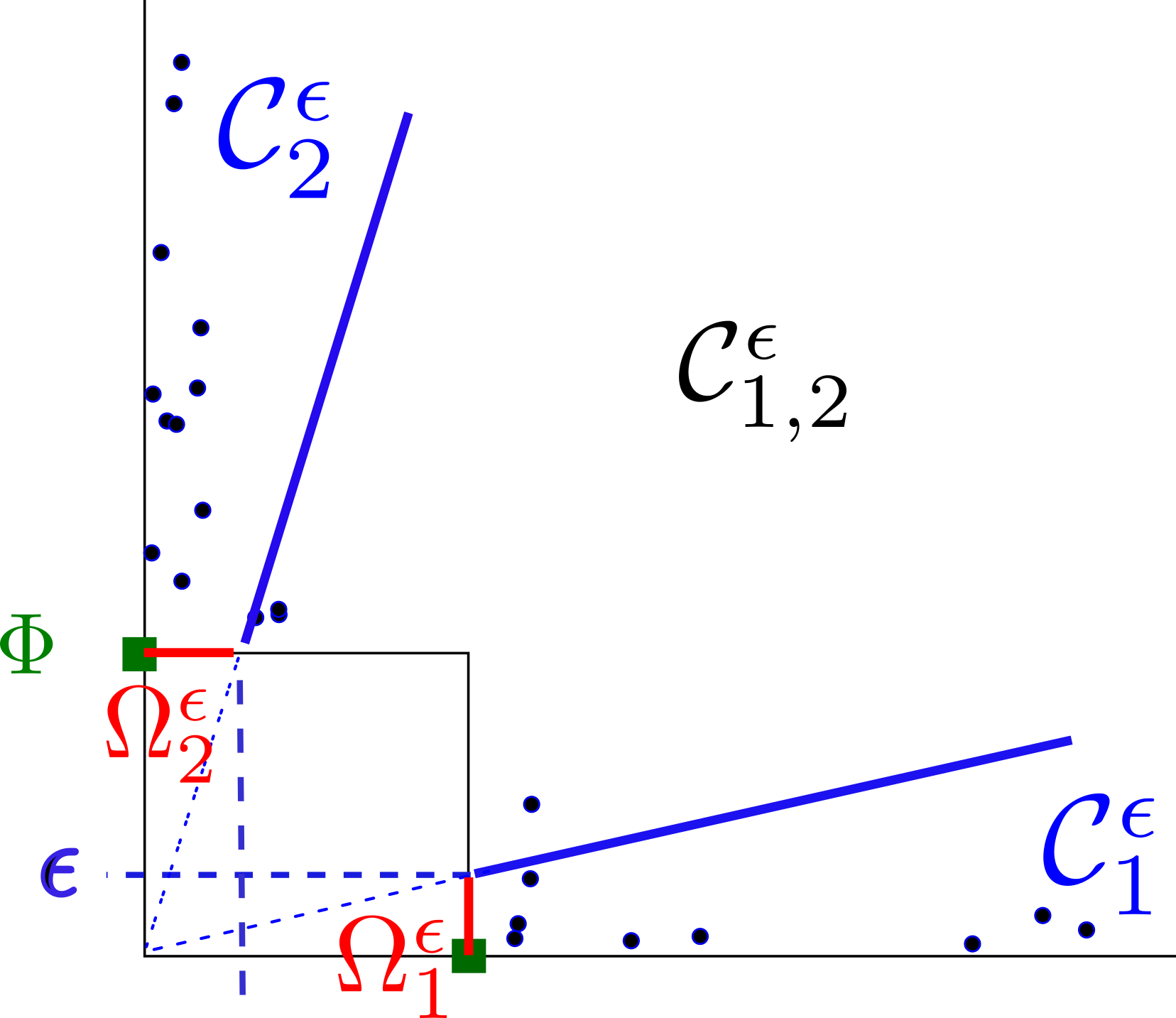
Figure 2: Truncated $\epsilon$-cones in 2D

Equivalently, the angular measure $\Phi$ defined in (10) decomposes as $\Phi~{}=~{}\sum_{\emptyset\subsetneq\alpha\subset\{1,\ldots,d\}}\Phi_{\alpha}$ corresponding to the partition $S_{d-1}^{\infty}=\coprod_{\emptyset\neq\alpha\subset\{1,\ldots,d\}}{\Omega}_{\alpha}$ of the unit sphere, where ${\Omega}_{\alpha}=S_{d-1}^{\infty}\cap{\mathcal{C}}_{\alpha}$. Our aim is to learn the support of $\mu$ or, more precisely, which cones have non-zero total mass $\mu(\mathcal{C}_{\alpha})=\Phi(\Omega_{\alpha})$. The next subsection shows that the $\mu_{n}^{\alpha,\epsilon}$’s introduced in Algorithm 1 are empirical estimators of the $\mu(\mathcal{C}_{\alpha})$’s.

3.2 Estimation of $\mu(\mathcal{C}_{\alpha})$

We point out that as soon as $\alpha\neq\{1,\ldots,d\}$, the cone $\mathcal{C}_{\alpha}$ is a subspace of zero Lebesgue measure. Real data, namely non-asymptotic data, generally do not concentrate on such sets, so that, if we were simply counting the points $\hat{V}_{i}$ in $\mathcal{C}_{\alpha}$, only the largest dimensional cone (the central one, corresponding to $\alpha=\{1,\ldots,d\})$ would have non zero mass. The idea is to introduce a tolerance parameter $\epsilon$ in order to capture the points whose projections on the unit sphere are $\epsilon$-close to the cone $\mathcal{C}_{\alpha}$, as illustrated in Fig. 2. This amounts to defining $\epsilon$-thickened faces on the sphere $S_{\infty}^{d-1}$, $\Omega_{\alpha}^{\epsilon}=\mathcal{C}_{\alpha}^{\epsilon}\cap S_{\infty}^{d-1}$ (the projections of the cones defined in (1) onto the sphere), so that

$$\Omega_{\alpha}^{\epsilon}=\big{\{}\mathbf{x}\in S_{d-1}^{\infty},~{}x_{i}>\epsilon\text{ for }i\in\alpha~{},~{}x_{i}\leq\epsilon\text{ for }i\notin\alpha\big{\}}.$$

A natural estimator of $\mu(\mathcal{C}_{\alpha})$ is thus $\mu_{n}(\mathcal{C}_{\alpha}^{\epsilon})=\mu_{n}^{\alpha,\epsilon}$, as defined in Section 2, see Eq. (2) therein. Thus, if $\mathbf{x}$ is a new observation, and if $\hat{T}(\mathbf{x})$ belongs to the $\epsilon$-thickened cone $\mathcal{C}^{\epsilon}_{\alpha}$ defined in (1), the scoring function $s_{n}(\mathbf{x})$ in (4) is in fact an empirical version of the quantity

$$\mathbb{P}(\mathbf{X}\in A_{\mathbf{x}}):=\mathbb{P}(T(\mathbf{X})\in\mathcal{C}_{\alpha},\|T(\mathbf{X})\|_{\infty}>\|T(\mathbf{x})\|).$$

Indeed, the latter is (using (9))

$$\mathbb{P}(\mathbf{V}\in\|T(\mathbf{x})\|_{\infty}\mathcal{C}_{\alpha}) ~{}~{}\simeq~{}~{}\|T(\mathbf{x})\|_{\infty}^{-1}\mu(\mathcal{C}_{\alpha})$$ (11)

$$~{}~{}\simeq~{}~{}\|\hat{T}(\mathbf{x})\|_{\infty}^{-1}\mu_{n}^{\alpha,\epsilon}~{}~{}=~{}~{}s_{n}(\mathbf{x})$$

It is beyond the scope of this paper to investigate upper bounds for $|\mu_{n}(\mathcal{C}_{\alpha}^{\epsilon})-\mu(\mathcal{C}_{\alpha})|$, which should be based on the decomposition: $|\mu_{n}(\mathcal{C}_{\alpha}^{\epsilon})-\mu(\mathcal{C}_{\alpha})|~{}~{}\leq~{}~{}|\mu_{n}-\mu|(\mathcal{C}_{\alpha}^{\epsilon})~{}~{}+~{}~{}|\mu(\mathcal{C}_{\alpha}^{\epsilon})-\mu(\mathcal{C}_{\alpha})|.$ The argument would be to investigate the first term in the right hand size by approximating the sub-cones $\mathcal{C}_{\alpha}^{\epsilon}$ by a Vapnik-Chervonenkis (VC) class of rectangles like in [9], where a non-asymptotic bound is stated on the estimation of the so-called stable tail dependence function (which is just another version of the exponent measure, using a standardization to uniform margins instead of Pareto margins). As for the second term, since $\mathcal{C}_{\alpha}^{\epsilon}$ and $\mathcal{C}_{\alpha}$ are close up to a volume proportional to $\epsilon^{d-|\alpha|}$, their mass can be proved close, under the condition that the density of $\mu|_{\mathcal{C}_{\alpha}}$ w.r.t. Lebesgue measure of dimension $|\alpha|$ on $\mathcal{C}_{\alpha}$ is bounded.

4 Experiments on simulated data

4.1 Simulation on 2D data

The purpose of this simulation is to provide an insight into the rationale of the algorithm in the bivariate case. Normal data are simulated under a 2D logistic distribution with asymmetric parameters (white and green points in Fig. 3), while the abnormal ones are uniformly distributed. Thus, the ‘normal’ extremes should be concentrated around the axes, while the ‘abnormal’ ones could be anywhere. The training set (white points) consists of normal observations. The testing set consists of normal observations (white points) and abnormal ones (red points). Fig. 3 represents the level sets of this scoring function (inversed colors, the darker, the more abnormal) in both the transformed and the non-transformed input space.

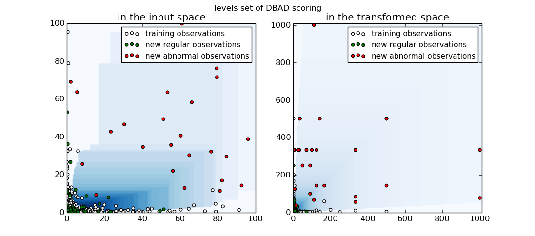
Figure 3: Level sets of $s_{n}$ on simulated 2D data

4.2 Recovering the support of the dependence structure

In this section, we simulate data whose asymptotic behavior corresponds to some exponent measure $\mu$. This measure is chosen such that it concentrates on $K$ chosen cones. Experiments illustrate in this case how many data is needed to recover properly the $K$ sub-cones (namely the dependence structure) depending on its complexity. If the dependence structure spreads on a high number $K$ of sub-cones, then a high number of data will be required.

Datasets of size $50000$ (resp. $150000$) are generated in $\mathbb{R}^{10}$ according to a popular multivariate extreme value model, introduced by [22], namely a multivariate asymmetric logistic distribution ($G_{log}$). The data have the following features: (i) They resemble ‘real life’ data, that is, the $X_{i}^{j}$’s are non zero and the transformed $\hat{V}_{i}$’s belong to the interior cone $\mathcal{C}_{\{1,\ldots,d\}}$ (ii) The associated (asymptotic) exponent measure concentrates on $K$ disjoint cones $\{\mathcal{C}_{\alpha_{m}},1\leq m\leq K\}$. For the sake of reproducibility, $G_{log}(\mathbf{x})=\exp\{-\sum_{m=1}^{K}\left(\sum_{j\in\alpha_{m}}(|A(j)|x_{j})^{-1/{w_{\alpha_{m}}}}\right)^{w_{\alpha_{m}}}\},$ where $|A(j)|$ is the cardinal of the set $\{\alpha\in D:j\in\alpha\}$ and where $w_{\alpha_{m}}=0.1$ is a dependence parameter (strong dependence). The data are simulated using Algorithm 2.2 in [20]. The subset of sub-cones $D$ with non-zero $\mu$-mass is randomly chosen (for each fixed number of sub-cones $K$) and the purpose is to recover $D$ by Algorithm 1. For each $K$, $100$ experiments are made and we consider the number of ‘errors’, that is, the number of non-recovered or false-discovered sub-cones. Table 1 shows the averaged numbers of errors among the $100$ experiments.

$\#$ sub-cones $K$	Aver. $\#$ errors	Aver. $\#$ errors
	(n=5e4)	(n=15e4)
3	0.07	0.01
5	0.00	0.01
10	0.01	0.06
15	0.09	0.02
20	0.39	0.14
25	1.12	0.39
30	1.82	0.98
35	3.59	1.85
40	6.59	3.14
45	8.06	5.23
50	11.21	7.87

Table 1: Support recovering on simulated data

The results are very promising in situations where the number of sub-cones is moderate w.r.t. the number of observations. Indeed, when the total number of sub-cones in the dependence structure is ‘too large’ (relatively to the number of observations), some sub-cones are under-represented and become ‘too weak’ to resist the thresholding (Step 4 in Algorithm 1). Handling complex dependence structures without a confortable number of observations thus requires a careful choice of the thresholding level $\mu_{\min}$, for instance by cross-validation.

5 Real-world data sets

5.1 Sparse structure of extremes (wave data)

Our goal is here to verify that the two expected phenomena mentioned in the introduction, 1- sparse dependence structure of extremes (small number of sub-cones with non zero mass), 2- low dimension of the sub-cones with non-zero mass, do occur with real data.

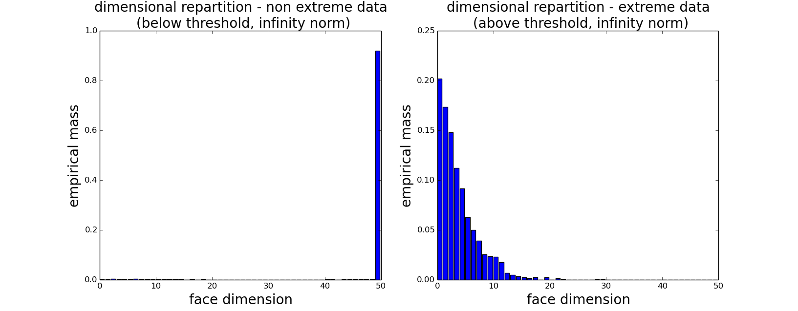
Figure 4: sub-cone dimensions of wave data

We consider wave directions data provided by Shell, which consist of $58585$ measurements $D_{i}$, $i\leq 58595$ of wave directions between $0^{\circ}$ and $360^{\circ}$ at $50$ different locations (buoys in North sea). The dimension is thus $50$. The angle $90^{\circ}$ being fairly rare, we work with data obtained as $X_{i}^{j}=1/(10^{-10}+|90-D_{i}^{j}|)$, where $D_{i}^{j}$ is the wave direction at buoy $j$, time $i$. Thus, $D_{i}^{j}$’s close to $90$ correspond to extreme $X_{i}^{j}$’s. Results in Table 2 ($\mu_{total}$ denotes the total probability mass of $\mu$) show that, the number of sub-cones $\mathcal{C}_{\alpha}$ identified by Algorithm 1 is indeed small compared to the total number of sub-cones ($2^{50}$-1) (Phenomenon 1). Extreme data are essentially concentrated in $18$ sub-cones. Further, the dimension of those sub-cones is essentially moderate (Phenomenon 2): respectively $93\%$, $98.6\%$ and $99.6\%$ of the mass is affected to sub-cones of dimension no greater than $10$, $15$ and $20$ respectively (to be compared with $d=50$). Histograms displaying the mass repartition produced by Algorithm 1 are given in Fig. 4.

	non-extreme	extreme
	data	data
$\#$ of sub-cones with positive
mass ($\mu_{\min}/\mu_{total}=0$)	3413	858
ditto after thresholding
($\mu_{\min}/\mu_{total}=0.002$)	2	64
ditto after thresholding
($\mu_{\min}/\mu_{total}=0.005$)	1	18

Table 2: Total number of sub-cones of wave data

5.2 Anomaly Detection

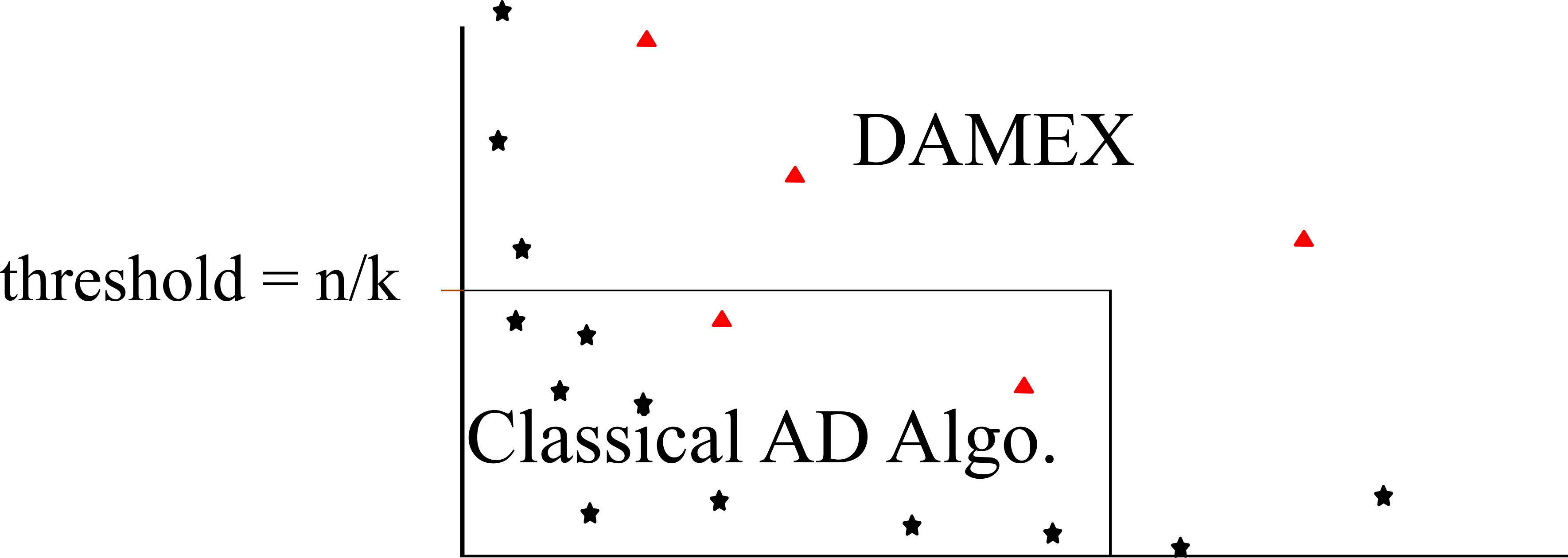
Figure 5: Combination of any AD algorithm with DAMEX

The main purpose of Algorithm 1 is to deal with extreme data. In this section we show that it may be combined with a standard AD algorithm to handle extreme and non-extreme data, improving the global performance of the chosen standard algorithm. This can be done as illustrated in Fig. 5 by splitting the input space between an extreme region and a non-extreme one, then applying Algorithm 1 to the extreme region, while the non-extreme one is processed with the standard algorithm.

One standard AD algorithm is the Isolation Forest (iForest) algorithm, which we chose in view of its established high performances ([15]). Our aim is to compare the results obtained with the combined method ‘iForest + DAMEX’ above described, to those obtained with iForest alone on the whole input space.

	number of samples	number of features
shuttle	85849	9
forestcover	286048	54
SA	976158	41
SF	699691	4
http	619052	3
smtp	95373	3

Table 3: Datasets characteristics

Six reference datasets in AD are considered: shuttle, forestcover, http, smtp, SF and SA. The experiments are performed in a semi-supervised framework (the training set consists of normal data). In a non-supervised framework (training set including abnormal data), the improvements brought by the use of DAMEX are less significant, but the precision score is still increased when the recall is high (high rate of true positives), inducing more vertical ROC curves near the origin.

The shuttle dataset is available in the UCI repository [14]. We use instances from all different classes but class $4$, which yields an anomaly ratio (class 1) of $7.15\%$. In the forestcover data, also available at UCI repository ([14]), the normal data are the instances from class $2$ while instances from class $4$ are anomalies,which yields an anomaly ratio of $0.9\%$. The last four datasets belong to the KDD Cup ’99 dataset ([12], [21]), which consist of a wide variety of hand-injected attacks (anomalies) in a closed network (normal background). Since the original demonstrative purpose of the dataset concerns supervised AD, the anomaly rate is very high ($80\%$). We thus transform the KDD data to obtain smaller anomaly rates. For datasets SF, http and smtp, we proceed as described in [23]: SF is obtained by picking up the data with positive logged-in attribute, and focusing on the intrusion attack, which gives $0.3\%$ of anomalies. The two datasets http and smtp are two subsets of SF corresponding to a third feature equal to ’http’ (resp. to ’smtp’). Finally, the SA dataset is obtained as in [8] by selecting all the normal data, together with a small proportion ($1\%$) of anomalies.

Table 3 summarizes the characteristics of these datasets. For each of them, 20 experiments on random training and testing datasets are performed, yielding averaged ROC and Precision-Recall curves whose AUC are presented in Table 4. The parameter $\mu_{\min}$ is fixed to $\mu_{total}/(\#$charged sub-cones), the averaged mass of the non-empty sub-cones.

Dataset	iForest only		iForest + DAMEX
	ROC	PR	ROC	PR
shuttle	0.996	0.974	$\mathbf{0.997}$	$\mathbf{0.987}$
forestcov.	0.964	0.193	$\mathbf{0.976}$	$\mathbf{0.363}$
http	0.993	0.185	$\mathbf{0.999}$	$\mathbf{0.500}$
smtp	$\mathbf{0.900}$	$\mathbf{0.004}$	0.898	0.003
SF	0.941	0.041	$\mathbf{0.980}$	$\mathbf{0.694}$
SA	0.990	0.387	$\mathbf{0.999}$	$\mathbf{0.892}$

Table 4: Results in terms of AUC

The parameters $(k,\epsilon)$ are chosen according to remarks 1 and 2. The stability w.r.t. $k$ (resp. $\epsilon$) is investigated over the range [$n^{1/4},n^{2/3}$] (resp. $[0.0001,0.1]$). This yields parameters $(k,\epsilon)=(n^{1/3},0.0001)$ for SA and forestcover, and $(k,\epsilon)=(n^{1/2},0.01)$ for shuttle. As the datasets http, smtp and SF do not have enough features to consider the stability, we choose the (standard) parameters $(k,\epsilon)=(n^{1/2},0.01)$. DAMEX significantly improves the precision for each dataset, excepting for smtp.

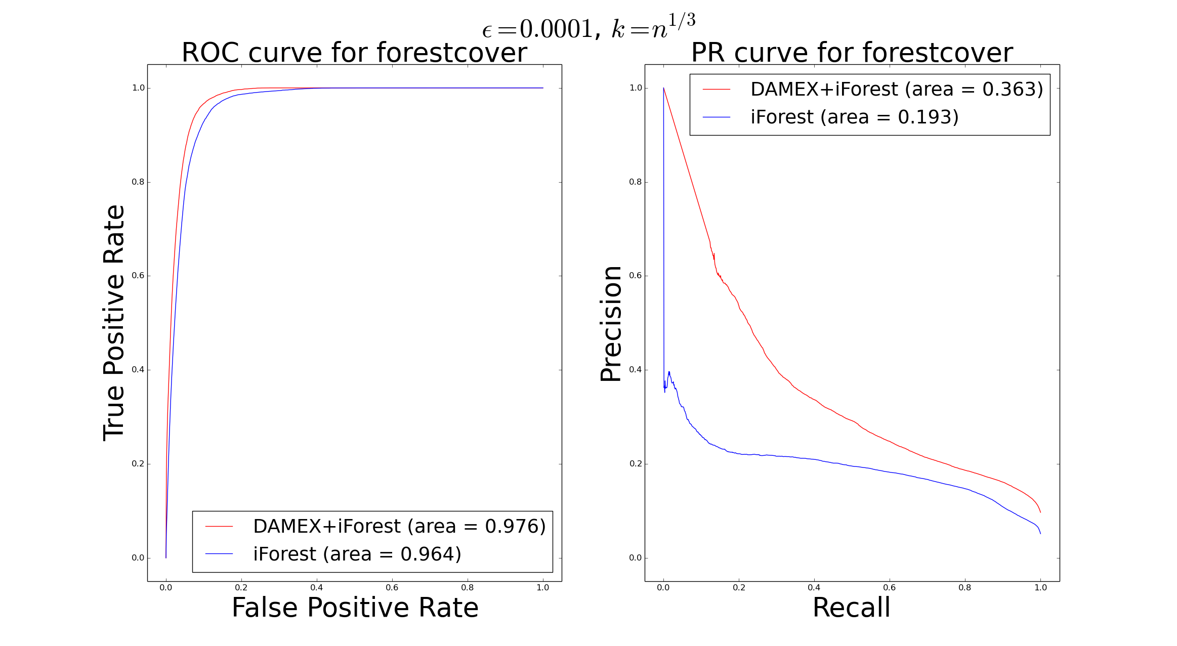
Figure 6: ROC and PR curve on forestcover dataset

Figure 7: ROC and PR curve on http dataset

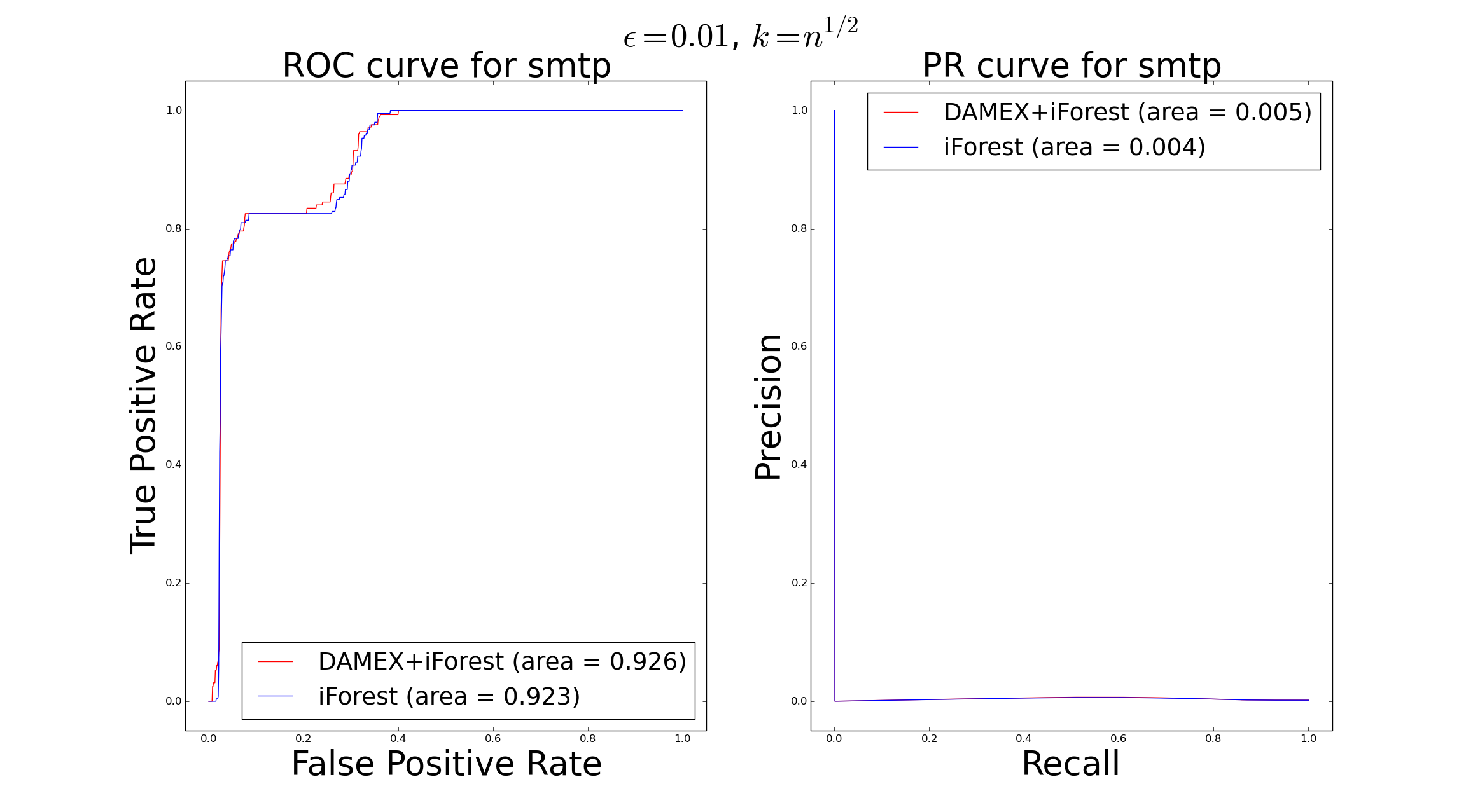
Figure 8: ROC and PR curve on smtp dataset

In terms of AUC of the ROC curve, one observes slight or negligible improvements. Figures 6, 7, 8, 9 represent averaged ROC curves and PR curves for forestcover, http, smtp and SF. The curves for the two other datasets are available in supplementary material. Excepting for the smtp dataset, one observes highter slope at the origin of the ROC curve using DAMEX. It illustrates the fact that DAMEX is particularly adapted to situation where one has to work with a low false positive rate constrain.

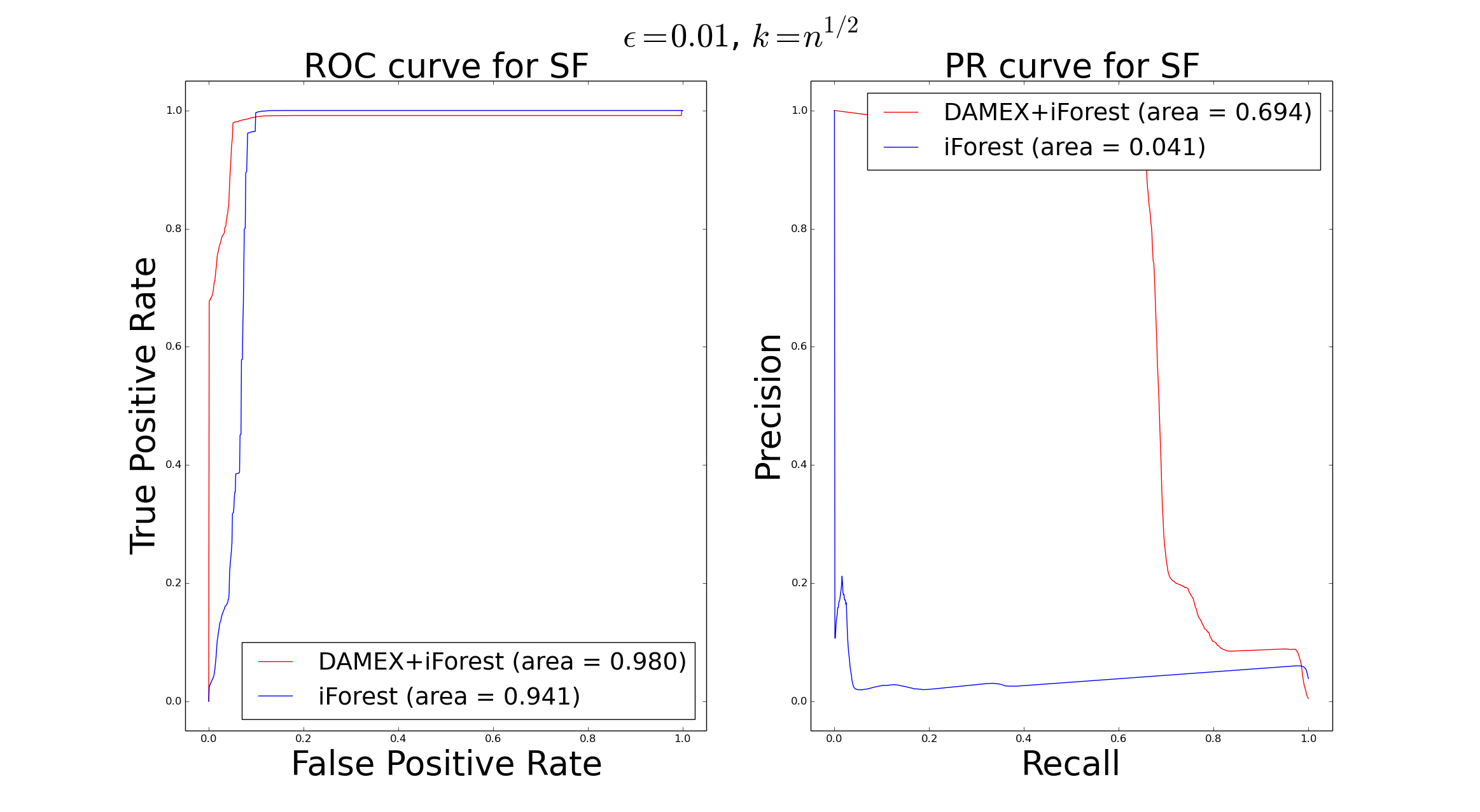
Figure 9: ROC and PR curve on SF dataset

Concerning the smtp dataset, the algorithm seems to be unable to capture any extreme dependence structure, either because the latter is non-existent (no regularly varying tail), or because the convergence is too slow to appear in our relatively small dataset.

6 Conclusion

The DAMEX algorithm allows to detect anomalies occurring in extreme regions of a possibly large-dimensional input space by identifying lower-dimensional subspaces around which normal extreme data concentrate. It is designed in accordance with well established results borrowed from multivariate Extreme Value Theory. Various experiments on simulated data and real Anomaly Detection datasets demonstrate its ability to recover the support of the extremal dependence structure of the data, thus improving the performance of standard Anomaly Detection algorithms. These results pave the way towards novel approaches in Machine Learning that take advantage of multivariate Extreme Value Theory tools for learning tasks involving features subject to extreme behaviors.

Acknowledgements

Part of this work has been supported by the industrial chair ‘Machine Learning for Big Data’ from Télécom ParisTech.

References

References

- [1] J. Beirlant, Y. Goegebeur, J. Teugels, and J. Segers. Statistics of Extremes: Theory and Applications. Wiley Series in Probability and Statistics. Wiley, 2004.
- [2] J. Beirlant, P. Vynckier, and J. L. Teugels. Tail index estimation, pareto quantile plots regression diagnostics. Journal of the American Statistical Association, 91(436):1659–1667, 1996.
- [3] S. Clémençon and J. Jakubowicz. Scoring anomalies: a M-estimation approach. In Proceedings of AISTATS, 2013.
- [4] D.A. Clifton, L. Tarassenko, N. McGrogan, D. King, S. King, and P. Anuzis. Bayesian extreme value statistics for novelty detection in gas-turbine engines. In Aerospace Conference, 2008 IEEE, pages 1–11, 2008.
- [5] David Andrew Clifton, Samuel Hugueny, and Lionel Tarassenko. Novelty detection with multivariate extreme value statistics. Journal of signal processing systems, 65(3):371–389, 2011.
- [6] S. Coles. An introduction to statistical modeling of extreme values. Springer Series in Statistics. Springer-Verlag, London, 2001.
- [7] L. de Haan and S.I. Resnick. Limit theory for multivariate sample extremes. Zeitschrift für Wahrscheinlichkeitstheorie und Verwandte Gebiete, 40(4):317–337, 1977.
- [8] E. Eskin, A. Arnold, M. Prerau, L. Portnoy, and S. Stolfo. A geometric framework for unsupervised anomaly detection. In Applications of data mining in computer security, pages 77–101. Springer, 2002.
- [9] N. Goix, A. Sabourin, and S. Clémençon. Learning the dependence structure of rare events: a non-asymptotic study. In Proceedings of the 28th Conference on Learning Theory, 2015.
- [10] N. Goix, A. Sabourin, and S. Clémençon. On anomaly ranking and excess-mass curves. In Proceedings of the Eighteenth International Conference on Artificial Intelligence and Statistics, page 287–295, 2015.
- [11] B. M. Hill. A simple general approach to inference about the tail of a distribution. Ann. Statist., 3(5):1163–1174, 09 1975.
- [12] KDDCup. The third international knowledge discovery and data mining tools competition dataset. KDD99-Cup http://kdd.ics.uci.edu/databases/kddcup99/kddcup99.html, 1999.
- [13] H.J. Lee and S.J. Roberts. On-line novelty detection using the kalman filter and extreme value theory. In Pattern Recognition, 2008. ICPR 2008. 19th International Conference on, pages 1–4, 2008.
- [14] M. Lichman. UCI machine learning repository, 2013.
- [15] F.T. Liu, K.M. Ting, and Z.H. Zhou. Isolation forest. In Data Mining, 2008. ICDM’08. Eighth IEEE International Conference on, pages 413–422, 2008.
- [16] S. Resnick. Extreme Values, Regular Variation, and Point Processes. Springer Series in Operations Research and Financial Engineering, 1987.
- [17] S.J. Roberts. Novelty detection using extreme value statistics. Vision, Image and Signal Processing, IEE Proceedings -, 146(3):124–129, Jun 1999.
- [18] S.J. Roberts. Extreme value statistics for novelty detection in biomedical signal processing. In Advances in Medical Signal and Information Processing, 2000. First International Conference on (IEE Conf. Publ. No. 476), pages 166–172, 2000.
- [19] R. L. Smith. Estimating tails of probability distributions. Ann. Statist., 15(3):1174–1207, 09 1987.
- [20] Alec Stephenson. Simulating multivariate extreme value distributions of logistic type. Extremes, 6(1):49–59, 2003.
- [21] M. Tavallaee, E. Bagheri, W. Lu, and A.A. Ghorbani. A detailed analysis of the kdd cup 99 data set. In Proceedings of the Second IEEE Symposium on Computational Intelligence for Security and Defence Applications 2009, 2009.
- [22] JA Tawn. Modelling multivariate extreme value distributions. Biometrika, 77(2):245–253, 1990.
- [23] K. Yamanishi, J.I. Takeuchi, G. Williams, and P. Milne. On-line unsupervised outlier detection using finite mixtures with discounting learning algorithms. In Proceedings of the sixth ACM SIGKDD international conference on Knowledge discovery and data mining, pages 320–324, 2000.