Queueing Analysis of a Large-Scale Bike Sharing System through Mean-Field Theory

Abstract

The bike sharing systems are fast increasing as a public transport mode in urban short trips, and have been developed in many major cities around the world. A major challenge in the study of bike sharing systems is that some large-scale and complex queueing networks have to be applied through multi-dimensional Markov processes, while their discussion always suffers a common difficulty: State space explosion. For this reason, this paper provides a mean-field computational method to study such a large-scale bike sharing system. Our mean-field computation is established in the following three steps: Firstly, a multi-dimensional Markov process is set up for expressing the states of the bike sharing system, and the empirical measure process of the multi-dimensional Markov process is given to partly overcome the difficulty of state space explosion. Based on this, the mean-field equations are derived by means of a virtual time-inhomogeneous $M(t)/M(t)/1/K$ queue whose arrival and service rates are determined by some mean-field computation. Secondly, the martingale limit is employed to investigate the limiting behavior of the empirical measure process, the fixed point is proved to be unique so that it can be computed by means of a nonlinear birth-death process, the asymptotic independence of this system is discussed, and specifically, these lead to numerical computation for the steady-state probability of the problematic (empty or full) stations. Finally, some numerical examples are given for valuable observation on how the steady-state probability of the problematic stations depends on some crucial parameters of the bike sharing system.

Keywords: Bike sharing system; queueing network; empirical measure process; mean-field equation; nonlinear birth-death process; martingale limit; fixed point; probability of problematic stations.

1 Introduction

The bike sharing systems are fast developing wide-spread adoption in major cities around the world, and are becoming a public mode of transportation devoted to short trips. Up to now, there have been more than 500 cities equipped with the bike sharing systems. Also, it is worth noting that the bike sharing systems are being regarded as a promising solution to jointly reducing, such as, traffic congestion, parking difficulty, transportation noise, air pollution and global warming. For a history overview of the bike sharing systems, readers may refer to, for instance, DeMaio [18] and Shaheen et al. [65] for more details. While DeMaio [16] provided a valuable prospect of the bike sharing systems in the 21st century. For the status of the bike sharing systems in some countries or cities, important examples include the United States by DeMaio and Gifford [17], France by Faye [21], the European cities with OBIS Project by Janett and Hendrik [36], London by Lathia et al. [40], Montreal by Morency et al. [57], Beijing by Liu et al. [52], several famous cities by Shu et al. [67], and further analysis by Shaheen et al. [64] and Meddin and DeMaio [55].

To understand the recent key research directions, here it is necessary to discuss some basic issues in design, operations and optimization of the bike sharing systems. The literature of bike sharing systems may be classified into two classes: The primary issues, and the higher issues. The primary issues are to discuss the number of stations, the station location, the number of bikes, the parking positions, and the types of bikes, all of which may be regarded as the strategic design. The higher issues are to analyze the demand prediction, the path scheduling, the inventory management, the repositioning (or rebalancing) by trucks, the price incentive, and applications of the intelligent information technologies. For analysis of the primary issues, readers may refer to, for example, Dell’Olio et al. [15], Lin and Yang [50], Kumar and Bierlaire [38], Martinez et al. [54] and Nair et al. [59]. While the higher issues were discussed by slightly more literature. Readers may refer to recent publications or technical reports for more details, among which are the repositioning by Forma et al. [22], Vogel and Mattfeld [72], Benchimol et al. [5], Raviv et al. [61], Contardo et al. [13], Caggiani and Ottomanelli [10], Fricker et al. [24], Chemla et al. [11], Shu et al. [67], Fricker and Gast [23] and Labadi et al. [39]; the inventory management by Lin et al. [51], Raviv and Kolka [61] and Schuijbroek et al. [66]; the price incentives by Waserhole and Jost [75], Waserhole et al. [78] and Fricker and Gast [23]; the fleet management by George and Xia [32, 31], Godfrey and Powell [33], Nair and Miller-Hooks [58] and Guerriero et al. [34]; the simulation models by Barth and Todd [3] and Fricker and Gast [23]; the data analysis by Froehlich and Oliver [26], Vogel et al [73], Borgnat et al. [8], Côme et al. [12] and Katzev [37].

Based on the above literature, it is necessary to further observe a basic solution to operations of the bike sharing systems. In a bike sharing system, a customer arrives at a station, takes a bike, and uses it for a while; then he returns the bike to a destination station. In general, the bikes are frequently distributed in an imbalanced manner among the stations, thus an arriving customer may always be confronted with two problematic cases: (1) A station is empty when a customer arrives at the station to rent a bike, and (2) a station is full when a bike-riding customer arrives at the station to return his bike. For the two problematic cases, the empty or full station is called a problematic station. Since a crucial question for the operational efficiency of the bike sharing system is its ability not only to meet the fluctuating demand for renting bikes at each station but also to provide enough vacant lockers to allow the renters to return the bikes at their destinations, the two types of problematic stations reflect a common challenge facing operations management of the bike sharing systems in practice due to the stochastic and time-inhomogeneous nature of the customer arrivals and bike returns. Therefore, it is a key to measuring the steady-state probability of the problematic stations in the study of bike sharing systems. Also, analysis of the steady-state probability of the problematic stations is useful and helpful in design, operations and optimization of the bike sharing systems in terms of numerical computation and comparison. Up to now, it is still difficult (and even impossible) to provide an explicit expression for the steady-state probability of the problematic stations because the bike sharing system is a more complicated closed queueing network with various geographical interactions, which come both from some bikes parked in multiple stations and from the other bikes ridden on multiple roads. For this, Section 2 explains that the bike sharing system is a Markov process of dimension $N^{2}$ through analysis of a complicated virtual closed queueing network, also see Li et al. [48] for more details.

To compute the steady-state probability of the problematic stations, it is better to develop a stochastic and dynamic method through applications of the queueing theory as well as Markov processes to the study of bike sharing systems. However, the available works on such a research direction are still few up to now. To survey the recent literature, some significant methods and results are listed as follows. The simple queues: Leurent [41] used the $M/M/1/C$ queue to consider a vehicle-sharing system in which each station contains an expanded waiting room only for those customers arriving at either a full station to return a bike or an empty station to rent a bike, and analyzed performance measures of this vehicle-sharing system in terms of a geometric distribution. Schuijbroek et al. [66] first computed the transient distribution of the $M/M/1/C$ queue, which is used to measure the service level in order to establish a mixed integer programming for the bike sharing system. Then they dealt with the inventory rebalancing and the vehicle routing by means of the optimal solution to the mixed integer programming. Raviv et al [61] and Raviv and Kolka [60] provided an effective method for computing the transient distribution of a time-inhomogeneous $M\left(t\right)/M\left(t\right)/1/C$ queue, which is used to evaluate the expected number of bike shortages at any station. The queueing networks: Savin et al. [63] used a loss network as well as the admission control to discuss capacity allocation of a rental model with two classes of customers, and studied the revenue management and fleet sizing decision. Adelman [1] applied a closed queueing network to propose an internal pricing mechanism for managing a fleet of service units, and also used a nonlinear flow model to discuss the price-based policy for the vehicle redistribution. George and Xia [32] provided an effective method of closed queueing networks in the study of vehicle rental systems, and determined the optimal number of parking spaces for each rental location. Li et al. [48] proposed a unified framework for analyzing the closed queueing networks in the study of bike sharing systems. The mean-field theory: Recently, the mean-field method as well as the queueing theory are applied to analyzing the bike sharing systems. Fricker et al. [24] considered a space-inhomogeneous bike sharing system, and expressed the minimal proportion of problematic stations within each cluster. Fricker and Gast [23] provided a detailed analysis for a space-homogeneous bike sharing system in terms of the $M/M/1/K$ queue and some simple mean-field models, and crucially, they gave the closed-form solution to the minimal proportion of problematic stations. Fricker and Tibi [25] first studied the central limit and local limit theorems for the independent (non identically distributed) random variables, which support analysis of a generalized Jackson network with product-form solution; then they used the limit theorems to give a better outline of the stationary asymptotic analysis of the locally space-homogeneous bike sharing systems. Li and Fan [47] developed numerical computation of the bike sharing systems under Markovian environment by means of the mean-field theory and the nonlinear QBD processes. The Markov decision processes: A simple closed queuing network is used to establish the Markov decision model in the study of bike sharing systems, and to provide a fluid approximation in order to compute the static optimal policy. Examples include Waserhole and Jost [75], Waserhole and Jost [78, 77] and Waserhole et al. [76].

For convenience of readers, it is necessary to recall some basic references in which the mean-field theory is applied to the analysis of large-scale stochastic systems. Readers may refer to Spitzer [68], Dawson [14], Sznitman [69], Vvedenskaya et al. [74], Mitzenmacher [56], Turner [71], Graham [29, 30], Benaim and Le Boudec [4], Gast and Gaujal [27, 28], Bordenave et al. [7], Li [43, 44], Li and Lui [49], Li et al. [45, 46], Fricker et al. [24] and Fricker and Tibi [25]. On the other hand, the metastability of Markov processes may be useful in the study of more general bike sharing systems when the nonlinear Markov processes are applied. Readers may refer to, such as, Bovier [9], Den Hollander [19], Antunes et al. [2], Tibi [70], Li [44] and more references therein.

The main contributions of this paper are twofold. The first contribution is to describe a mean-field queueing model to analyze the large-scale bike sharing systems, where the arrival, walk, bike-riding (or return) processes among the stations are given some simplified assumptions whose purpose is to guarantee applicability of the mean-field theory. For this, we develop a mean-field queueing method combining the mean-field theory with the time-inhomogeneous queue, the martingale limits and the nonlinear birth-death processes. To this end, we provide a complete picture of applying the mean-field theory to the study of bike sharing systems through four basic steps: (1) The system of mean-field equations is set up by means of a virtual time-inhomogeneous $M(t)/M(t)/1/K$ queue whose arrival and service rates are determined by means of some mean-field computation; (2) the asymptotic independence (or propagation of chaos) is proved in terms of the martingale limit and the uniqueness of the fixed point; (3) numerical computation of the fixed point is given by using a system of nonlinear equations corresponding to the nonlinear birth-death processes; and (4) performance analysis of the bike sharing system is given through some numerical computation.

The second contribution of this paper is to provide a detailed analysis for computing the steady-state probability of the problematic stations, which is one of the most key measures in the study of bike sharing systems. It is worth noting that the service level, optimal design and control mechanism of bike sharing systems can be computed by means of the steady-state probability of the problematic stations. Therefore, this paper develops effective algorithms for computing the steady-state probability of the problematic stations, and gives a numerically computational framework in the study of bike sharing systems. Furthermore, we use some numerical examples to give valuable observation and understanding on how the performance measures depend on some crucial parameters of the bike sharing system. On the other hand, in view that Fricker et al. [24], Fricker and Gast [23], Fricker and Tibi [25] and Li and Fan [47] are the only important references that are closely related to this paper by using the mean-field theory, but differently, this paper provides more work focusing on some key theoretical points such as the virtual time-inhomogeneous $M(t)/M(t)/1/K$ queue, the mean-field equations, the martingale limits, the nonlinear birth-death processes, numerical computation of the fixed point, and numerical analysis for the steady-state probability of the problematic stations. With successful exposition of the key theoretical points, such a numerical computation can greatly enable a broad study of bike sharing systems. Therefore, the methodology and results of this paper gain new insights on how to establish the mean-field queueing models for discussing more general bike sharing systems by means of the mean-field theory, the time-inhomogeneous queues and the nonlinear Markov processes.

The remainder of this paper is organized as follows. In Section 2, we first describe a large-scale bike sharing system with $N$ identical stations, give a $N$-dimensional Markov process for expressing the states of the bike sharing system, and establish an empirical measure process of the $N$-dimensional Markov process in order to partly overcome the difficulty of state space explosion. In Section 3, we set up a system of mean-field equations satisfied by the expected fraction vector through a virtual time-inhomogeneous $M(t)/M(t)/1/K$ queue whose arrival and service rates are determined by means of some mean-field computation. In Section 4, we establish a Lipschitz condition, and prove the existence and uniqueness of solution to the system of mean-field equations. In Section 5, we provide a martingale limit of the sequences of empirical measure Markov processes in the bike sharing system. In Section 6, we analyze the fixed point of the system of mean-field equations, and prove that the fixed point is unique. Based on this, we simply analyze the asymptotic independence of the bike sharing system, and also discuss the limiting interchangeability with respect to $N\rightarrow\infty$ and $t\rightarrow+\infty$. In Section 7, we provide some effective computation of the fixed point, and use some numerical examples to investigate how the steady-state probability of the problematic stations depends on some crucial parameters of the bike sharing system. Some concluding remarks are given in Section 8.

2 Model Description

In this section, we first describe a large-scale bike sharing system with $N$ identical stations, and establish a $N$-dimensional Markov process for expressing the states of the bike sharing system. To overcome the difficulty of state space explosion, we provide an empirical measure process of the $N$-dimensional Markov process.

We first show that a bike sharing system can be modeled as a complex stochastic system whose analysis is always difficult and challenging. Then we explain the reasons why it is necessary to develop some simplified models in the study of bike sharing systems. In particular, we indicate that the mean-field theory plays a key role in establishing and analyzing such a simplified model whose purpose is to be able to set up some basic and useful relations among several key parameters of system.

A Complex Stochastic System

In the bike sharing system, a customer arrives at a station, takes a bike, and uses it for a while; then he returns the bike to any station and immediately leaves this system. Based on this, if the bike sharing system has $N$ stations for $N\geq 2$, then it can contain at most $N\left(N-1\right)$ roads because there may be a road between any two stations. When the stations and roads are different and heterogeneous, Li et al. [48] showed that the bike sharing system can be modeled as a complicated closed queueing network due to the fact that the total number of bikes is fixed in this system. In this case, the bikes are regarded as the virtual customers, while the stations and the roads are viewed as the virtual servers. Based on this, the closed queueing network is described as a Markov process $\left\{\overrightarrow{\mathfrak{n}}\left(t\right):t\geq 0\right\}$ of dimension $N^{2}$, where

$$\overrightarrow{\mathfrak{n}}\left(t\right)=\left(\mathbf{n}_{1}\left(t\right),\mathbf{n}_{2}\left(t\right),\ldots,\mathbf{n}_{N}\left(t\right)\right),$$

$$\mathbf{n}_{k}\left(t\right)=\left(n_{k}\left(t\right);n_{k,1}\left(t\right),\ldots,n_{k,k-1}\left(t\right),n_{k,k+1}\left(t\right),\ldots,n_{k,N}\left(t\right)\right),$$

$$\sum_{k=1}^{N}n_{k}\left(t\right)+\sum_{i=1}^{N}\sum_{j\neq i}^{N}n_{i,j}\left(t\right)=\Re,$$

$n_{k}\left(t\right)$ is the number of bikes parked at Station $k$, $n_{k,j}\left(t\right)$ is the number of bikes rided on Road $k\rightarrow j$ for $j\neq k$ and $1\leq j,k\leq N$, and $\Re$ is the total number of bikes in the bike sharing system.

In general, analysis of the Markov process $\left\{\overrightarrow{\mathfrak{n}}\left(t\right):t\geq 0\right\}$ of dimension $N^{2}$ is usually difficult due to at least three reasons: (1) The state space explosion for a large integer $N$, (2) the complex routes among the virtual servers which are either the $N$ stations or the $N\left(N-1\right)$ roads, and (3) a complicated expression for the steady-state probability distribution of joint queue lengths. See Li and Fan [48] for more details. For this, it is necessary in practice to provide a simplified model that contains only several key parameters of system, while the simplified model is used to set up some basic and useful relations among the key parameters. Crucially, not only do the basic relations support numerical computation of the steady-state probability of the problematic stations, but they are also helpful for performance analysis of the bike sharing system. To provide such a simplified model, the remainder of this paper will provide a mean-field queueing model described from the bike sharing system.

A Basic Condition to Apply the Mean-Field Theory

To apply the mean-field theory, we only need to consider the bike information $(n_{1}\left(t\right),n_{2}\left(t\right)$, $\ldots,n_{N}\left(t\right))$ on the $N$ stations, while the bike information of the $N\left(N-1\right)$ roads will be combined into the ‘probabilistic behavior’ of the random vector $\left(n_{1}\left(t\right),n_{2}\left(t\right),\ldots,n_{N}\left(t\right)\right)$ by means of some mean-field computation. See Theorem 1 and its proof in the next section. At the same time, a basic condition is also needed to guarantee the exchangeability of the $N$-dimensional Markov process $\left\{\left(n_{1}\left(t\right),n_{2}\left(t\right),\ldots,n_{N}\left(t\right)\right):t\geq 0\right\}$, that is, for any permutation $\left(i_{1},i_{2},i_{3},\ldots,i_{N}\right)$ of $\left(1,2,3,\ldots,N\right)$,

$$P\left\{n_{1}\left(t\right)=k_{1},n_{2}\left(t\right)=k_{2},\ldots,n_{N}\left(t\right)=k_{N}\right\}=P\left\{n_{i_{1}}\left(t\right)=k_{i_{1}},n_{i_{2}}\left(t\right)=k_{i_{2}},\ldots,n_{i_{N}}\left(t\right)=k_{i_{N}}\right\}.$$

See Li [44] for the mean-field analysis of big networks. In fact, the following assumption (1) that the bike sharing system consists of $N$ identical stations guarantee the exchangeability of the Markov process $\left\{\left(n_{1}\left(t\right),n_{2}\left(t\right),\ldots,n_{N}\left(t\right)\right):t\geq 0\right\}$ so that the mean-field theory can be applied to discussing the bike sharing system.

Although the model assumptions to apply mean-field theory are simplified greatly, we can still set up some useful and basic relations among several key parameters of system, and also provide some simple and effective algorithms both for computing the steady-state probability of the problematic stations and for analyzing performance measures of the bike sharing system.

Simplified Model Assumptions

Based on the above analysis, we make some necessarily simplified assumptions for applying the mean-field theory to studying the bike sharing system as follows:

(1) The $N$ identical stations: The bike sharing system consists of $N$ identical stations, each of which has a finite bike capacity. At the initial time $t=0$, each station contains $C$ bikes and $K$ positions to park the bikes, where $1\leq C<K<\infty$.

(2) The arrive processes: The arrivals of outside customers at the bike sharing system are a Poisson process with arrival rate $N\lambda$ for $\lambda>0$.

(3) The walk processes: If an outside or walking customer arrives at an empty station in which no bike may be rented, then he has to walk to another station again in the hope of renting a bike. We assume that the customer may rent a bike from a station within at most $\omega$ consequent walks, otherwise he will directly leave this system (that is, if he has not rented a bike after $\omega$ consequent walks yet). Note that one walk is viewed as a process that the customer walks from an empty station to another station, and $\omega$ is the maximal number of consequent walks of the customer among the stations.

We assume that the walk times between any two stations are all exponential with walk rate $\gamma>0$. Obviously, the expected walk time is $1/\gamma$.

(4) The bike-riding (or return) processes: If a bike-riding customer arrives at a full station in which no parking position is available, then he has to ride the bike to another station again. We assume that the returning-bike process is persistent in the sense that the customer must find a station with an empty position to return his bike (that is, he can not leave this system before his bike is returned), because the bike is the public property so that no one can make it his own.

We assume that the bike-riding times between any two stations are all exponential with bike-riding rate $\mu$ for $\gamma\leq\mu<+\infty$. Clearly, the expected bike-riding time is $1/\mu$.

(5) The departure discipline: The customer departure has two different cases: (a) The customer directly leaves the bike sharing system if he has not rented a bike yet after $\omega$ consequent walks; or (b) once one customer takes, uses and returns the bike to a station, he completes this trip, thus he can immediately leave the bike sharing system.

We assume that the arrival, walk and bike-riding processes are independent, and all the above random variables are independent of each other. Note that the randomly bike-riding and walk times show that the road length between any two stations is considered in this paper. For such a bike sharing system, Figure 1 provides some physical interpretation.

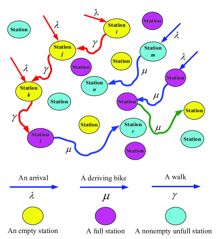
Figure 1: The physical interpretation of a bike sharing system

Remark 1

(1) The assumption of the $N$ identical stations is used to guarantee applicability of the mean-field theory, that is, the $N$-dimensional Markov process $\{(n_{1}\left(t\right),n_{2}\left(t\right),\ldots$, $n_{N}\left(t\right)):t\geq 0\}$ is exchangeable. Although the model assumptions to apply the mean-field theory are simplified greatly (note that several key parameters of system will be observed and analyzed in a simple form), we can still set up some useful and basic relations among the key parameters of system, and also find some valuable law and pattern both from computing the steady-state probability of the problematic stations and from analyzing performance measures of the bike sharing system.

(2) It is necessary to explain the maximal number $\omega$ of consequent walks of the customer. If $\omega=0$, then the arriving customer immediately leaves this system once he arrives at a full station. If $\omega$ is smaller, then the customer would like to find an available bike at a lucky station through at most $\omega$ consequent walks, because a bike can help him to promptly deal with a number of important things so that he would like to accept the time delay due to the hope of renting a bike within at most $\omega$ consequent walks.

(3) The road lengths among the $N$ stations are considered here, while the bike-riding time on any road is exponential with bike-riding rate $\mu$. Based on this, the road length is measured by means of the randomly bike-riding time. In addition, the assumption with $0<\gamma<\mu<+\infty$ makes sense in practice because the riding bike is faster than the walk on any road. On the other hand, the assumptions on the i.i.d. bike-riding times and on the i.i.d. walk times are to guarantee applicability of the mean-field theory, that is, the $N$-dimensional Markov process $\left\{\left(n_{1}\left(t\right),n_{2}\left(t\right),\ldots,n_{N}\left(t\right)\right):t\geq 0\right\}$ is exchangeable. Therefore, the $N$ identical stations also contain their identically physical factors under a random setting.

In the remainder of this section, we first establish a $N$-dimensional Markov process for expressing the states of the bike sharing system. Then we give an empirical measure process of the $N$-dimensional Markov process in order to overcome the difficulty of state space explosion.

Let $X_{i}^{\left(N\right)}\left(t\right)$ be the number of bikes parked in Station $i$ at time $t\geq 0$. Then $X_{i}^{\left(N\right)}\left(t\right)=n_{i}\left(t\right)$, and henceforth we only use the notation $X_{i}^{\left(N\right)}\left(t\right)$. It is easy to see from the above model descriptions that $\mathcal{X}=\left\{\left(X_{1}^{\left(N\right)}\left(t\right),X_{2}^{\left(N\right)}\left(t\right),\ldots,X_{N}^{\left(N\right)}\left(t\right)\right):t\geq 0\right\}$ is a $N$-dimensional Markov process. In general, it is always more difficult to directly study the $N$-dimensional Markov process $\mathcal{X}$ due to the state space explosion. Thus we need to introduce an empirical measure process of the $N$-dimensional Markov process $\mathcal{X}$ as follows. We write

$$Y_{k}^{\left(N\right)}\left(t\right)=\frac{1}{N}\sum_{i=1}^{N}\mathbf{1}_{\left\{X_{i}^{\left(N\right)}\left(t\right)=k\right\}},$$

where $\mathbf{1}_{\left\{\cdot\right\}}$ is an indicator function. Obviously, $Y_{k}^{\left(N\right)}\left(t\right)$ is the proportion of the stations with $k$ bikes at time $t$, and $0\leq\sum_{i=1}^{N}\mathbf{1}_{\left\{X_{i}^{\left(N\right)}\left(t\right)=k\right\}}\leq N$. Let

$$\mathbf{Y}^{\left(N\right)}\left(t\right)=\left(Y_{0}^{\left(N\right)}\left(t\right),Y_{1}^{\left(N\right)}\left(t\right),...,Y_{K-1}^{\left(N\right)}\left(t\right),Y_{K}^{\left(N\right)}\left(t\right)\right).$$

Then it is easy to see that the empirical measure process $\left\{\mathbf{Y}^{\left(N\right)}\left(t\right):t\geq 0\right\}$ is a Markov process on the state space $\Omega=\left[0,1\right]^{K+1}$.

To study the empirical measure Markov process, we write

$$y_{k}^{\left(N\right)}\left(t\right)=E\left[Y_{k}^{\left(N\right)}\left(t\right)\right]$$

and

$$\mathbf{y}^{\left(N\right)}\left(t\right)=\left(y_{0}^{\left(N\right)}\left(t\right),y_{1}^{\left(N\right)}\left(t\right),...,y_{K-1}^{\left(N\right)}\left(t\right),y_{K}^{\left(N\right)}\left(t\right)\right).$$

3 The Mean-Field Equations

In this section, we first describe the bike sharing system as a virtual time-inhomogeneous $M(t)/M(t)/1/K$ queue whose arrival and service rates are determined by means of the mean-field theory. Then we set up a system of mean-field equations, which is satisfied by the expected fraction vector $\mathbf{y}^{\left(N\right)}\left(t\right)$, in terms of the virtual time-inhomogeneous $M(t)/M(t)/1/K$ queue.

Note that the $N$ stations are identical according to the above model description on both system parameters and operations discipline, thus we can use the mean-field theory to study the bike sharing system. In this case, we only need to observe a tagged station (for example, Station 1) whose number of bikes is regarded as a virtual time-inhomogeneous $M(t)/M(t)/1/K$ queue (see Figure 2); while the other $N-1$ stations have some impact on the tagged station, and the impact can be analyzed by means of the empirical measure process through a mean-field computation for the new arrival and service rates in this virtual queue. Specifically, we also explain the reason why the new arrival and service processes in this virtual queue are time-inhomogeneous. See Figure 2 for more details.

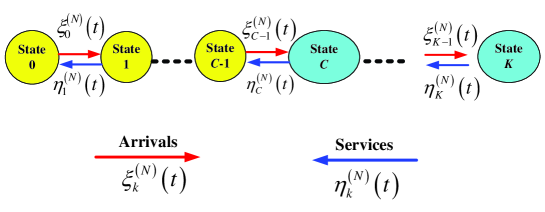
Figure 2: The state transitions in the $M(t)/M(t)/1/K$ queue

It is necessary to explain the difference of the arrival and service processes between the bike sharing system and the virtual time-inhomogeneous $M(t)/M(t)/1/K$ queue. For example, if a real customer arrives and rents a bike at a tagged station, then the number of bikes parked in the tagged station decreases by one, thus the real customer arrivals at the tagged station should be a part of the service process of the $M(t)/M(t)/1/K$ queue; while if a real customer returns a bike to a tagged station and leaves this system (i.e., his trip is completed), then the number of bikes parked in the tagged station increases by one, thus the real customers’ returning their bikes to the tagged station should be a part of the arrival process of the $M(t)/M(t)/1/K$ queue. Furthermore, the following Theorem 1 provides a more detailed analysis for various parts of the arrival and service processes in the virtual time-inhomogeneous $M(t)/M(t)/1/K$ queue.

For the time-inhomogeneous $M(t)/M(t)/1/K$ queue, now we use the mean-field theory to discuss its Poisson input with arrival rate $\xi_{l}^{\left(N\right)}\left(t\right)$ for $0\leq l\leq K-1$ and its exponential service times with service rate $\eta_{k}^{\left(N\right)}\left(t\right)$ for $1\leq k\leq K$.

The following theorem provides expressions for the arrival and service rates: $\xi_{l}^{\left(N\right)}\left(t\right)$ for $0\leq l\leq K-1$ and $\eta_{k}^{\left(N\right)}\left(t\right)$ for $1\leq k\leq K$, respectively. Note that the time-inhomogeneous arrival and service rates will play a key role in our mean-field study later.

Theorem 1

For $1\leq k\leq K$ and $\omega=0,1,2,\ldots$, we have

$$\eta_{k}^{\left(N\right)}\left(t\right)=\eta^{\left(N\right)}\left(t\right)=\lambda+\gamma y_{0}^{\left(N\right)}\left(t\right)\frac{1-\left[y_{0}^{\left(N\right)}\left(t\right)\right]^{\omega}}{1-y_{0}^{\left(N\right)}\left(t\right)}.$$ (1)

At the same time, for $0\leq l\leq K-1$ we have

$$\xi_{l}^{\left(N\right)}\left(t\right)=\left\{\begin{array}[c]{ll}\frac{\mu}{N}\frac{1}{1-y_{K}^{\left(N\right)}\left(t\right)}\left\{\left(C-l\right)+\left(N-1\right)\left[C-\sum_{k=1}^{K}ky_{k}^{\left(N\right)}\left(t\right)\right]\right\},&0\leq l\leq C-1,\\ \frac{\mu}{N}\frac{1}{1-y_{K}^{\left(N\right)}\left(t\right)}\left\{\left(N-1\right)\left[C-\sum_{k=1}^{K}ky_{k}^{\left(N\right)}\left(t\right)\right]\right\},&C\leq l\leq K-1.\end{array}\right.$$ (2)

Proof  We first prove Equation (1). In this case, we need to specifically deal with State $0$. If one customer arrives at an empty station, then the customer has to walk from the empty station to another station. It is easy to see that the bikes parked at the tagged station will have two different cases: (a) There is at least one bike with probability $\sum_{i=1}^{K}y_{i}^{\left(N\right)}\left(t\right)$; and (b) there is no bike with probability $y_{0}^{\left(N\right)}\left(t\right)$. For Case (a), the customer can rent a bike for his trip; while for Case (b), the customer will have to walk to another station again until he hopes to be able to rent a bike from a next station within the $\omega$ consequent walks. Notice that the role played by State $0$ is depicted in Figure 3, thus we can easily observe that the state transitions from State $0$ are jointly caused by the arrival, walk and return (or bike-riding) processes.

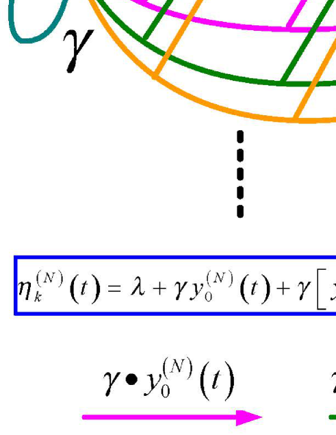
Figure 3: The state transitions for computing $\eta_{k}^{\left(N\right)}\left(t\right)$

To compute the service rate $\eta_{k}^{\left(N\right)}\left(t\right)$ for $1\leq k\leq K$, it is seen from Figure 3 that State $0$ (that is, the tagged station is empty) is a key, and it leads to the rate $\gamma\left[y_{0}^{\left(N\right)}\left(t\right)\right]^{n}$ with respect to $n$ consequent walks, where the $n$ consequent walks correspond to $n$ empty stations with probability $\left[y_{0}^{\left(N\right)}\left(t\right)\right]^{n}$for $1\leq n\leq\omega$. In the final walk with $n=\omega$, either the customer rents a bike at a nonempty station, or he directly leaves the bike sharing system if no bike is rented after $\omega$ consequent walks. Thus the number of the consequent walks to find an available station may be $1$ with probability $y_{0}^{\left(N\right)}\left(t\right)$, $2$ with $\left[y_{0}^{\left(N\right)}\left(t\right)\right]^{2}$, and generally, $n$ with $\left[y_{0}^{\left(N\right)}\left(t\right)\right]^{n}$ for $1\leq n\leq\omega$. Based on this, for the virtual time-inhomogeneous $M(t)/M(t)/1/K$ queue, we obtain its service rates in States $k$ for $1\leq k\leq K$ as follows:

$$\eta_{k}^{\left(N\right)}\left(t\right) =\lambda+\gamma y_{0}^{\left(N\right)}\left(t\right)+\gamma\left[y_{0}^{\left(N\right)}\left(t\right)\right]^{2}+\gamma\left[y_{0}^{\left(N\right)}\left(t\right)\right]^{3}+\cdots+\gamma\left[y_{0}^{\left(N\right)}\left(t\right)\right]^{\omega}$$

$$=\lambda+\gamma y_{0}^{\left(N\right)}\left(t\right)\frac{1-\left[y_{0}^{\left(N\right)}\left(t\right)\right]^{\omega}}{1-y_{0}^{\left(N\right)}\left(t\right)}$$

$$=\eta^{\left(N\right)}\left(t\right),$$

which is independent of the number $k=1,2,\ldots,K$.

Now, we prove Equation (2) in terms of the mean-field theory. Note that we can compute the arrival rates $\xi_{l}^{\left(N\right)}\left(t\right)$ for $0\leq l\leq K-1$ according to a detailed probability analysis on States $l$ for $0\leq l\leq K-1$.

For $l=0$ (i.e., States $0$), all the original $C$ bikes in the tagged station are rented to travel on the roads. For the other $N-1$ stations, our computation for the number of bikes rented to travel on the roads is based on the mean-field theory (i.e., under an average setting), thus the expected number of bikes rented to travel on the roads is given by

$$\left(N-1\right)\cdot\left[C-\sum_{k=1}^{K}ky_{k}^{\left(N\right)}\left(t\right)\right],$$

where $\sum_{k=1}^{K}ky_{k}^{\left(N\right)}\left(t\right)$ is the expected number of bikes parked in the tagged station, while $C-\sum_{k=1}^{K}ky_{k}^{\left(N\right)}\left(t\right)$ is the expected number of bikes rented to travel on the roads from the tagged station. Therefore, for the $N$ stations, the total expected number of bikes rented to travel on the roads is given by

$$C+\left(N-1\right)\cdot\left[C-\sum_{k=1}^{K}ky_{k}^{\left(N\right)}\left(t\right)\right].$$

Note that the returning-bike process of each bike is persistent in the sense that the customer keeps finding an empty position in the next station, it is easy to check that the return rate of each riding bike arriving at the tagged station is given by

$$\mu+\mu y_{K}^{\left(N\right)}\left(t\right)+\mu\left[y_{K}^{\left(N\right)}\left(t\right)\right]^{2}+\mu\left[y_{K}^{\left(N\right)}\left(t\right)\right]^{3}+\cdots=\mu\frac{1}{1-y_{K}^{\left(N\right)}\left(t\right)},$$

where $\left[y_{K}^{\left(N\right)}\left(t\right)\right]^{n}$ is the probability that a customer $n$ times continuously returns his bike to $n$ full stations. Thus we use the mean-field computation to obtain that for State 0 (for $l=0$),

$$\xi_{0}^{\left(N\right)}\left(t\right) =\frac{1}{N}\left\{C+\left(N-1\right)\left[C-\sum_{k=1}^{K}ky_{k}^{\left(N\right)}\left(t\right)\right]\right\}\cdot\mu\frac{1}{1-y_{K}^{\left(N\right)}\left(t\right)}$$

$$=\frac{\mu}{N}\frac{1}{1-y_{K}^{\left(N\right)}\left(t\right)}\left\{C+\left(N-1\right)\left[C-\sum_{k=1}^{K}ky_{k}^{\left(N\right)}\left(t\right)\right]\right\}.$$

Similarly, for States $l$ with $1\leq l\leq C-1$, we have

$$\xi_{l}^{\left(N\right)}\left(t\right)=\frac{\mu}{N}\frac{1}{1-y_{K}^{\left(N\right)}\left(t\right)}\left\{\left(C-l\right)+\left(N-1\right)\left[C-\sum_{k=1}^{K}ky_{k}^{\left(N\right)}\left(t\right)\right]\right\}.$$

Finally, for States $l$ with $C\leq l\leq K$, since all the original $C$ bikes are parked in the tagged station, we obtain

$$\xi_{l}^{\left(N\right)}\left(t\right)=\frac{\mu}{N}\frac{1}{1-y_{K}^{\left(N\right)}\left(t\right)}\left\{\left(N-1\right)\left[C-\sum_{k=1}^{K}ky_{k}^{\left(N\right)}\left(t\right)\right]\right\},$$

which is independent of the number $l=C,C+1,\ldots,K$. This completes this proof.  

Remark 2

(1) In Equation (1), for the number of consequent walks, it may be useful to observe two special cases: (a) If $\omega=0$, $\eta_{k}^{\left(N\right)}\left(t\right)=\lambda$. (b) If $\omega\rightarrow\infty$, then $\eta_{k}^{\left(N\right)}\left(t\right)=\lambda+\gamma y_{0}^{\left(N\right)}\left(t\right)/\left[1-y_{0}^{\left(N\right)}\left(t\right)\right]$.

(2) The time-inhomogeneous $M(t)/M(t)/1/K$ queue is a fictitious queueing system corresponding to the number of bikes parked in the tagged station, while its virtual arrival and virtual service rates are determined by means of the empirical measure process through some mean-field computation.

(3) It is seen from the proof of Theorem 1 that the different ages of “finding-bike attempts” and “returning-bike attempts” has not any influence on the mean-field computation due to the memoryless property of the exponential distributions and of the Poisson processes. Thus, the mean-field method can be successfully applied to our current analysis of the bike sharing system. However, it will be very difficult (or an open problem) to apply the mean-field method if there exist general distributions or general renewal processes in the bike sharing system.

In the remainder of this section, we set up a system of mean-field equations by means of the time-inhomogeneous $M(t)/M(t)/1/K$ queue whose state transition relation is depcited in Figure 2 with the arrival rate $\xi_{l}^{\left(N\right)}\left(t\right)$ for $0\leq l\leq K-1$, and with service rate $\eta_{k}^{\left(N\right)}\left(t\right)=\eta^{\left(N\right)}\left(t\right)$ for $1\leq k\leq K$. To establish such mean-field equations, readers nay refer to, such as, Li and Lui [49], Li et al. [45, 46] and Fricker and Gast [23] for more details.

To apply the mean-field theory, the number of bikes parked in the tagged station is described as the virtual time-inhomogeneous $M(t)/M(t)/1/K$ queue. Thus we can set up a system of mean-field equations in terms of the (nonlinear) birth-death process corresponding to the $M(t)/M(t)/1/K$ queue. To this end, we denote by $Q\left(t\right)$ the queue length of the $M(t)/M(t)/1/K$ queue at time $t\geq 0$. Then it is seen from Figure 2 that $\left\{Q\left(t\right):t\geq 0\right\}$ is a time-inhomogeneous continuous-time birth-death process whose infinite generator is given by

$$\mathbf{V}_{\mathbf{y}^{\left(N\right)}\left(t\right)}=\left(\begin{array}[c]{cccccc}B_{1}\left(t\right)&B_{0}\left(t\right)&&&&\\ B_{2}\left(t\right)&-\Theta_{C}^{\left(N\right)}\left(t\right)&\xi_{C}^{\left(N\right)}\left(t\right)&&&\\ &\eta^{\left(N\right)}\left(t\right)&-\Theta_{C}^{\left(N\right)}\left(t\right)&\xi_{C}^{\left(N\right)}\left(t\right)&&\\ &&\ddots&\ddots&\ddots&\\ &&&\eta^{\left(N\right)}\left(t\right)&-\Theta_{C}^{\left(N\right)}\left(t\right)&\xi_{C}^{\left(N\right)}\left(t\right)\\ &&&&\eta^{\left(N\right)}\left(t\right)&-\eta^{\left(N\right)}\left(t\right)\end{array}\right),$$ (3)

where

$$\eta^{\left(N\right)}\left(t\right)=\lambda+\gamma y_{0}^{\left(N\right)}\left(t\right)\frac{1-\left[y_{0}^{\left(N\right)}\left(t\right)\right]^{\omega}}{1-y_{0}^{\left(N\right)}\left(t\right)},$$

for $0\leq l\leq C$

$$\xi_{l}^{\left(N\right)}\left(t\right)=\frac{\mu}{N}\frac{1}{1-y_{K}^{\left(N\right)}\left(t\right)}\left\{\left(C-l\right)+\left(N-1\right)\left[C-\sum_{k=1}^{K}ky_{k}^{\left(N\right)}\left(t\right)\right]\right\}$$

and

$$\Theta_{l}^{\left(N\right)}\left(t\right)=\xi_{l}^{\left(N\right)}\left(t\right)+\eta^{\left(N\right)}\left(t\right);$$

$$B_{1}\left(t\right)=\left(\begin{array}[c]{ccccc}-\xi_{0}^{\left(N\right)}\left(t\right)&\xi_{0}^{\left(N\right)}\left(t\right)&&&\\ \eta^{\left(N\right)}\left(t\right)&-\Theta_{1}^{\left(N\right)}\left(t\right)&\xi_{1}^{\left(N\right)}\left(t\right)&&\\ &\ddots&\ddots&\ddots&\\ &&\eta^{\left(N\right)}\left(t\right)&-\Theta_{C-2}^{\left(N\right)}\left(t\right)&\xi_{C-2}^{\left(N\right)}\left(t\right)\\ &&&\eta^{\left(N\right)}\left(t\right)&-\Theta_{C-1}^{\left(N\right)}\left(t\right)\end{array}\right)_{C\times C},$$

$$B_{0}\left(t\right)=\left(0,0,\ldots,0,\xi_{C-1}^{\left(N\right)}\left(t\right)\right)^{T}$$

and

$$B_{2}\left(t\right)=\left(0,0,\ldots,0,\eta^{\left(N\right)}\left(t\right)\right),$$

$A^{T}$ denotes the transpose of the vector (or matrix) $A$.

Using the birth-death process described in Figure 2, we obtain a system of mean-field (or ordinary differential) equations as follows:

$$\frac{\text{d}}{\text{d}t}y_{0}^{\left(N\right)}\left(t\right)=-\xi_{0}^{\left(N\right)}\left(t\right)y_{0}^{\left(N\right)}\left(t\right)+\eta^{\left(N\right)}\left(t\right)y_{1}^{\left(N\right)}\left(t\right),$$

for $1\leq k\leq K-1$

$$\frac{\text{d}}{\text{d}t}y_{k}^{\left(N\right)}\left(t\right)=\xi_{k-1}^{\left(N\right)}\left(t\right)y_{k-1}^{\left(N\right)}\left(t\right)-\left[\xi_{k}^{\left(N\right)}\left(t\right)+\eta^{\left(N\right)}\left(t\right)\right]y_{k}^{\left(N\right)}\left(t\right)+\eta^{\left(N\right)}\left(t\right)y_{k+1}^{\left(N\right)}\left(t\right),$$

$$\frac{\text{d}}{\text{d}t}y_{K}^{\left(N\right)}\left(t\right)=\xi_{K-1}^{\left(N\right)}\left(t\right)y_{K-1}^{\left(N\right)}\left(t\right)-\eta^{\left(N\right)}\left(t\right)y_{K}^{\left(N\right)}\left(t\right).$$

Now, we write the above system of mean-field equations in a vector form as

$$\frac{\text{d}}{\text{d}t}\mathbf{y}^{\left(N\right)}\left(t\right)=\mathbf{y}^{\left(N\right)}\left(t\right)\mathbf{V}_{\mathbf{y}^{\left(N\right)}\left(t\right)},$$ (4)

with the boundary and initial conditions

$$\mathbf{y}^{\left(N\right)}\left(t\right)e=1,\text{ \ }\mathbf{y}^{\left(N\right)}\left(0\right)=\mathbf{g,}$$ (5)

where $\mathbf{g}=\left(g_{0},g_{1},\ldots,g_{K}\right)$ with $g_{i}\geq 0$ for $0\leq i\leq K$ and $\sum_{i=0}^{K}g_{i}=1$, and $e$ is a column vector of ones with a suitable dimension in the context.

Remark 3

To deal with the time-inhomogeneous continuous-time birth-death process, readers may refer to Chapter 8 in Li [42] for more details, where the detailed literatures are surveyed both for the time-inhomogeneous queues and for the time-inhomogeneous Markov processes.

4 A Lipschitz Condition

In this section, we first establish a Lipschitz condition. Then we prove the existence and uniqueness of solution to the system of ordinary differential equations by means of the Lipschitz condition.

We write

$$\frac{\text{d}}{\text{d}t}\mathbf{y}\left(t\right)=\mathbf{y}\left(t\right)\mathbf{V}_{\mathbf{y}\left(t\right)},$$ (6)

with the boundary and initial conditions

$$\mathbf{y}\left(t\right)e=1,\text{ \ }\mathbf{y}\left(0\right)=\mathbf{g},$$ (7)

where

$$\mathbf{V}_{\mathbf{y}\left(t\right)}=\left(\begin{array}[c]{ccccc}-a\left(t\right)&a\left(t\right)&&&\\ b\left(t\right)&-c\left(t\right)&a\left(t\right)&&\\ &\ddots&\ddots&\ddots&\\ &&b\left(t\right)&-c\left(t\right)&a\left(t\right)\\ &&&b\left(t\right)&-b\left(t\right)\end{array}\right),$$ (8)

$$b\left(t\right)=\lambda+\gamma y_{0}\left(t\right)\frac{1-\left[y_{0}\left(t\right)\right]^{\omega}}{1-y_{0}\left(t\right)},$$

$$a\left(t\right)=\mu\frac{1}{1-y_{K}\left(t\right)}\left[C-\sum_{k=1}^{K}ky_{k}\left(t\right)\right]$$

and

$$c\left(t\right)=a\left(t\right)+b\left(t\right).$$

Obviously, that Equations (6) and (7) are a system of first-order ordinary differential equations.

Remark 4

Note that the system of ordinary differential equations (6) and (7) is the limiting version of Equations (4) and (5) as $N\rightarrow\infty$, while the existence of the limit $\lim_{N\rightarrow\infty}\mathbf{y}^{\left(N\right)}\left(t\right)=\mathbf{y}\left(t\right)$ will be proved in the next section according to the martingale limits and the weak convergence in the Skorohod space.

To discuss the existence and uniqueness of solution to the system of ordinary differential equations (6) and (7), in what follows we need to establish a Lipschitz condition by means of a computational method given in Section 4.1 of Li et al. [45].

For simplicity of description, we first suppress time $t$ from the vector $\mathbf{y}\left(t\right)$ and its entries $y_{k}\left(t\right)$ for $0\leq k\leq K$. Then we rewrite Equations (6) and (7) in a simple form as

$$\frac{\text{d}}{\text{d}t}\mathbf{y}=F\left(\mathbf{y}\right),\text{ \ \ \ \ }\mathbf{y}e\mathbf{=1,y}\left(0\right)=\mathbf{g},$$ (9)

where

$$F\left(\mathbf{y}\right)=\mathbf{yV}_{\mathbf{y}}=\left(y_{0},y_{1},\ldots,y_{K}\right)\left(\begin{array}[c]{ccccc}-a&a&&&\\ b&-c&a&&\\ &\ddots&\ddots&\ddots&\\ &&b&-c&a\\ &&&b&-b\end{array}\right),$$

$$b=\lambda+\frac{\gamma y_{0}\left(1-y_{0}^{\omega}\right)}{1-y_{0}},\text{ \ \ }a=\frac{\mu}{1-y_{K}}\left(C-\sum_{k=1}^{K}ky_{k}\right),$$

$$c=\frac{\mu}{1-y_{K}}\left(C-\sum_{k=1}^{K}ky_{k}\right)+\left(\lambda+\frac{\gamma y_{0}\left(1-y_{0}^{\omega}\right)}{1-y_{0}}\right).$$

Let

$$F\left(\mathbf{y}\right)=\left(F_{0}\left(\mathbf{y}\right),F_{1}\left(\mathbf{y}\right),\ldots,F_{K-1}\left(\mathbf{y}\right),F_{K}\left(\mathbf{y}\right)\right).$$

Then for $k=0$

$$F_{0}\left(\mathbf{y}\right)=-y_{0}\frac{\mu}{1-y_{K}}\left(C-\sum_{k=1}^{K}ky_{k}\right)+y_{1}\left[\lambda+\frac{\gamma y_{0}\left(1-y_{0}^{\omega}\right)}{1-y_{0}}\right],$$

for $1\leq i\leq K-1$

$$F_{k}\left(\mathbf{y}\right)=\left(y_{i-1}-y_{i}\right)\frac{\mu}{1-y_{K}}\left(C-\sum_{k=1}^{K}ky_{k}\right)+\left(y_{i}-y_{i+1}\right)\left[\lambda+\frac{\gamma y_{0}\left(1-y_{0}^{\omega}\right)}{1-y_{0}}\right]$$

and for $k=K$

$$F_{K}\left(\mathbf{y}\right)=y_{K-1}\frac{\mu}{1-y_{K}}\left(C-\sum_{k=1}^{K}ky_{k}\right)-y_{K}\left[\lambda+\frac{\gamma y_{0}\left(1-y_{0}^{\omega}\right)}{1-y_{0}}\right].$$

Now, we define the norms of a vector $\mathbf{x=}\left(x_{0},x_{1},\ldots,x_{K}\right)$ and a matrix $A=\left(a_{i,j}\right)_{0\leq i,j\leq K}$ as follows:

$$\left\|\mathbf{x}\right\|=\max_{0\leq i\leq K}\left\{\left|x_{i}\right|\right\}$$

and

$$\left\|A\right\|=\max_{0\leq j\leq K}\left\{\sum_{i=0}^{K}\left|a_{i,j}\right|\right\}.$$

It is easy to check that

$$\left\|\mathbf{x}A\right\|\leq\left\|\mathbf{x}\right\|\left\|A\right\|.$$

From (41) of Li et al. [45], the matrix of partial derivatives of the vector function $F\left(\mathbf{y}\right)$ of dimension $K+1$ is given by

$$DF\left(\mathbf{y}\right)=\left(\begin{array}[c]{cccc}\frac{\partial F_{0}\left(\mathbf{y}\right)}{\partial y_{0}}&\frac{\partial F_{1}\left(\mathbf{y}\right)}{\partial y_{0}}&\cdots&\frac{\partial F_{K}\left(\mathbf{y}\right)}{\partial y_{0}}\\ \frac{\partial F_{0}\left(\mathbf{y}\right)}{\partial y_{1}}&\frac{\partial F_{1}\left(\mathbf{y}\right)}{\partial y_{1}}&\cdots&\frac{\partial F_{K}\left(\mathbf{y}\right)}{\partial y_{1}}\\ \vdots&\vdots&&\vdots\\ \frac{\partial F_{0}\left(\mathbf{y}\right)}{\partial y_{K}}&\frac{\partial F_{1}\left(\mathbf{y}\right)}{\partial y_{K}}&&\frac{\partial F_{K}\left(\mathbf{y}\right)}{\partial y_{K}}\end{array}\right).$$ (10)

To establish the Lipschitz condition of the vector function $F\left(\mathbf{y}\right)$ of dimension $K+1$, it is seen from Lemma 5 of Li et al. [45] that we need to provide an upper bound of the norm $\left\|DF\left(\mathbf{y}\right)\right\|$. To this end, it is necessary to first give an assumption with respect to the two key numbers $y_{0}$ and $y_{K}$ as follows:

Assumption of Problematic Stations: Let $\delta$ be a sufficiently small positive number. We assume that $0\leq y_{0},y_{K}\leq 1-\delta$.

Now, we provide some interpretation for practical rationality of the Assumption of Problematic Stations. Firstly, the probability $y_{0}\left(t\right)+y_{K}\left(t\right)$ of problematic stations is always smaller by means of some management mechanism or control methods (for example, repositioning by trucks, price incentives, and applications of information technologies), thus it is natural and rational to take the condition: $0\leq y_{0},y_{K}\leq 1-\delta$ in practice. Secondly, Theorem 5 in Section 6 will further demonstrate from the steady-state viewpoint that $\lim_{t\rightarrow+\infty}y_{0}\left(t\right)=p_{0}\leq 1/2$ and $\lim_{t\rightarrow+\infty}y_{K}\left(t\right)=p_{K}\leq 1-\delta$. Finally, if $y_{0}\left(t\right)=1$, then $y_{k}\left(t\right)=0$ for $1\leq k\leq K$; while if $y_{K}\left(t\right)=1$, then $y_{k}\left(t\right)=0$ for $0\leq k\leq K-1$. Therefore, such a case with either $y_{0}\left(t\right)=1$ or $y_{K}\left(t\right)=1$ will directly lead to the unavailability of the bike sharing system.

Theorem 2

(1) Under the Assumption of Problematic Stations, $\left\|DF\left(\mathbf{y}\right)\right\|\leq\mathbf{M}$, where

$$\mathbf{M}=2\lambda+\gamma\frac{\omega\left(\omega+5\right)}{2}+\frac{\mu}{\delta}\left[\left(1+\frac{1}{\delta}\right)C+\frac{K\left(K+1\right)}{2}\right]\mathbf{.}$$

(2) The the vector function $F\left(\mathbf{y}\right)$ of dimension $K+1$ is continuous and also satisfies the Lipschitz condition for $\left(t,\mathbf{y}\right)\in[0,+\infty)\times\left\{[0,1-\delta]\times\left[0,1\right]^{K-1}\times[0,1-\delta]\right\}$.

(3) There exists a unique solution to the system of ordinary differential equations $\frac{\text{d}}{\text{d}t}\mathbf{y}=F\left(\mathbf{y}\right)$, $\mathbf{y}e=1$ and $\mathbf{y}\left(0\right)=\mathbf{g}$ for $\left(t,\mathbf{y}\right)\in[0,+\infty)\times\left\{[0,1-\delta]\times\left[0,1\right]^{K-1}\times[0,1-\delta]\right\}$.

Proof:  (1) It follows from (10) that

$$\left\|DF\left(\mathbf{y}\right)\right\|=\max_{0\leq j\leq K}\left\{\sum_{i=0}^{K}\left|\frac{\partial F_{j}\left(\mathbf{y}\right)}{\partial y_{i}}\right|\right\}.$$

It is easy to check that

$$\frac{\partial F_{0}\left(\mathbf{y}\right)}{\partial y_{0}}=-\frac{\mu}{1-y_{K}}\left(C-\sum_{k=1}^{K}ky_{k}\right)+\gamma y_{1}\sum_{k=1}^{\omega-1}ky_{0}^{k},$$

$$\frac{\partial F_{0}\left(\mathbf{y}\right)}{\partial y_{1}}=y_{0}\frac{\mu}{1-y_{K}}+\lambda+\gamma y_{0}\sum_{k=0}^{\omega-1}y_{0}^{k},$$

and for $2\leq i\leq K$

$$\frac{\partial F_{0}\left(\mathbf{y}\right)}{\partial y_{i}}=y_{0}\frac{i\mu}{1-y_{K}}.$$

By using

$$\left|y_{k}\right|\leq 1,0\leq k\leq K;\text{ \ }\frac{1}{1-y_{K}}\leq\frac{1}{\delta};\text{ \ }0\leq C-\sum_{k=1}^{K}ky_{k}\leq C,$$

we obtain

$$\sum_{i=0}^{K}\left|\frac{\partial F_{0}\left(\mathbf{y}\right)}{\partial y_{i}}\right|\leq\lambda+\frac{\mu}{\delta}\left(C+\frac{K\left(K+1\right)}{2}\right)+\gamma\frac{\omega\left(\omega+3\right)}{2}.$$

Similarly, we obtain that for $1\leq j\leq K-1$

$$\sum_{i=0}^{K}\left|\frac{\partial F_{j}\left(\mathbf{y}\right)}{\partial y_{i}}\right|\leq 2\lambda+\frac{\mu}{\delta}\left(2C+\frac{K\left(K+1\right)}{2}\right)+\gamma\frac{\omega\left(\omega+5\right)}{2}$$

and

$$\sum_{i=0}^{K}\left|\frac{\partial F_{K}\left(\mathbf{y}\right)}{\partial y_{i}}\right|\leq\lambda+\frac{\mu}{\delta}\left[\left(1+\frac{1}{\delta}\right)C+\frac{K\left(K+1\right)}{2}\right]+\gamma\frac{\omega\left(\omega+3\right)}{2}.$$

Let

$$\mathbf{M}=2\lambda+\gamma\frac{\omega\left(\omega+5\right)}{2}+\frac{\mu}{\delta}\left[\left(1+\frac{1}{\delta}\right)C+\frac{K\left(K+1\right)}{2}\right].$$

Then

$$\left\|DF\left(\mathbf{y}\right)\right\|=\max_{0\leq j\leq K}\left\{\sum_{i=0}^{K}\left|\frac{\partial F_{j}\left(\mathbf{y}\right)}{\partial y_{i}}\right|\right\}\leq\mathbf{M}.$$

(2) By means of Lemma 5 in Li et al. [45], we obtain that for any two vectors $\mathbf{x,y\in}[0,1-\delta]\times\left[0,1\right]^{K-1}\times[0,1-\delta]$,

$$\left\|F\left(\mathbf{x}\right)-F\left(\mathbf{y}\right)\right\|\leq\sup_{0\leq\widetilde{t}\leq 1}\left\|DF\left(\mathbf{x+}\widetilde{t}\left(\mathbf{y-x}\right)\right)\right\|\left\|\mathbf{y-x}\right\|\leq\mathbf{M}\left\|\mathbf{y-x}\right\|.$$

This shows that $F\left(\mathbf{y}\right)$ is continuous and also satisfies the Lipschitz condition for $\left(t,\mathbf{y}\right)\in[0,+\infty)\times\left\{[0,1-\delta]\times\left[0,1\right]^{K-1}\times[0,1-\delta]\right\}$.

(3) Note that $F\left(\mathbf{y}\right)$ is continuous and also satisfies the Lipschitz condition for $\left(t,\mathbf{y}\right)\in[0,+\infty)\times\left\{[0,1-\delta]\times\left[0,1\right]^{K-1}\times[0,1-\delta]\right\}$, it follows from Chapter 1 of Hale [35] that there exists a unique solution to the system of ordinary differential equations $\frac{\text{d}}{\text{d}t}\mathbf{y}=F\left(\mathbf{y}\right)$, $\mathbf{y}e=1$ and $\mathbf{y}\left(0\right)=\mathbf{g}$ for $\left(t,\mathbf{y}\right)\in[0,+\infty)\times\left\{[0,1-\delta]\times\left[0,1\right]^{K-1}\times[0,1-\delta]\right\}$. This completes the proof.  

In the remainder of this section, we set up a simple relation between the two systems of ordinary differential equations (4) and (5); and (6) and (7) through a limiting assumption $\lim_{N\rightarrow\infty}\mathbf{y}^{\left(N\right)}\left(t\right)=\mathbf{y}\left(t\right)$, the correctness of which will further be proved in the next section. To this end, from Equation (4) we set

$$G\left(\mathbf{y}^{\left(N\right)}\left(t\right)\right)=\mathbf{y}^{\left(N\right)}\left(t\right)\mathbf{V}_{\mathbf{y}^{\left(N\right)}\left(t\right)}$$

or a simple form by suppressing $t$

$$G\left(\mathbf{y}^{\left(N\right)}\right)=\mathbf{y}^{\left(N\right)}\mathbf{V}_{\mathbf{y}^{\left(N\right)}}.$$

It follows from (4) and (5) that

$$\frac{\text{d}}{\text{d}t}\mathbf{y}^{\left(N\right)}=G\left(\mathbf{y}^{\left(N\right)}\right),\text{ \ }\mathbf{y}^{\left(N\right)}e=1.$$

By using $\lim_{N\rightarrow\infty}\mathbf{y}^{\left(N\right)}\left(t\right)=\mathbf{y}\left(t\right)$, we obtain that for $0\leq k\leq K-1$

$$\lim_{N\rightarrow\infty}\xi_{k}^{\left(N\right)}\left(t\right)=a\left(t\right),$$

and

$$\lim_{N\rightarrow\infty}\eta^{\left(N\right)}\left(t\right)=b\left(t\right).$$

Thus comparing the vector $G\left(\mathbf{y}^{\left(N\right)}\right)$ with the vector $F\left(\mathbf{y}\right)$, we obtain

$$\lim_{N\rightarrow\infty}G\left(\mathbf{y}^{\left(N\right)}\right)=F\left(\mathbf{y}\right).$$

Since

$$\frac{\text{d}}{\text{d}t}\left(\lim_{N\rightarrow\infty}\mathbf{y}^{\left(N\right)}\left(t\right)\right)=\frac{\text{d}}{\text{d}t}\mathbf{y=}F\left(\mathbf{y}\right)$$

and

$$\lim_{N\rightarrow\infty}\left(\frac{\text{d}}{\text{d}t}\mathbf{y}^{\left(N\right)}\left(t\right)\right)=\lim_{N\rightarrow\infty}G\left(\mathbf{y}^{\left(N\right)}\right)\mathbf{=}F\left(\mathbf{y}\right),$$

we obtain

$$\frac{\text{d}}{\text{d}t}\left(\lim_{N\rightarrow\infty}\mathbf{y}^{\left(N\right)}\left(t\right)\right)=\lim_{N\rightarrow\infty}\left(\frac{\text{d}}{\text{d}t}\mathbf{y}^{\left(N\right)}\left(t\right)\right).$$

5 The Martingale Limit

In this section, we provide a martingale limit (i.e., the weak convergence in the Skorohod space) for the sequence of empirical measure Markov processes in the bike sharing system.

We define a $\left(K+1\right)$-dimensional simplex

$$\mathcal{F}=\left\{f=\left(f_{0},f_{1},\ldots,f_{K-1},f_{K}\right):f_{k}\geq 0\text{ and }\sum\limits_{k=0}^{K}f_{k}=1\right\},$$

and endow $\mathcal{F}$ with the metric

$$d\left(x,y\right)=\sup_{0\leq k\leq K}\frac{\left|x_{k}-y_{k}\right|}{k+1},\text{ \ }x,y\in\mathcal{F}.$$

Obviously, $d\left(x,y\right)\leq 1$ for $x,y\in\mathcal{F}$. Under the metric, the space $\mathcal{F}$ is compact, complete and separable. Let $D_{\mathcal{F}}[0,+\infty)$ be the space of right-continuous paths with left limits in $\mathcal{F}$ endowed with the Skorohod metric. For the Skorohod space and the weak convergence, readers may refer to Billingsley [6] and Chapter 3 of Ethier and Kurtz [20] for more details.

For the the empirical measure $\mathbf{Y}^{\left(N\right)}\left(t\right)$, we write

$$\mathbf{W}\left(\mathbf{Y}^{\left(N\right)}\left(t\right)\right)=\left(\begin{array}[c]{cccccc}A_{1}^{\left(N\right)}\left(t\right)&A_{0}^{\left(N\right)}\left(t\right)&&&&\\ A_{2}^{\left(N\right)}\left(t\right)&-\Gamma_{C}^{\left(N\right)}\left(t\right)&\alpha_{C}^{\left(N\right)}\left(t\right)&&&\\ &\beta^{\left(N\right)}\left(t\right)&-\Gamma_{C}^{\left(N\right)}\left(t\right)&\alpha_{C}^{\left(N\right)}\left(t\right)&&\\ &&\ddots&\ddots&\ddots&\\ &&&\beta^{\left(N\right)}\left(t\right)&-\Gamma_{C}^{\left(N\right)}\left(t\right)&\alpha_{C}^{\left(N\right)}\left(t\right)\\ &&&&\beta^{\left(N\right)}\left(t\right)&-\beta^{\left(N\right)}\left(t\right)\end{array}\right),$$

where

$$\beta^{\left(N\right)}\left(t\right)=\lambda+\gamma Y_{0}^{\left(N\right)}\left(t\right)\frac{1-\left[Y_{0}^{\left(N\right)}\left(t\right)\right]^{\omega}}{1-Y_{0}^{\left(N\right)}\left(t\right)},$$

for $0\leq l\leq C$

$$\alpha_{l}^{\left(N\right)}\left(t\right)=\frac{\mu}{N}\frac{1}{1-Y_{K}^{\left(N\right)}\left(t\right)}\left\{\left(C-l\right)+\left(N-1\right)\left[C-\sum_{k=1}^{K}kY_{k}^{\left(N\right)}\left(t\right)\right]\right\}$$

and

$$\Gamma_{l}^{\left(N\right)}\left(t\right)=\alpha_{l}^{\left(N\right)}\left(t\right)+\beta^{\left(N\right)}\left(t\right);$$

$$A_{1}^{\left(N\right)}\left(t\right)=\left(\begin{array}[c]{ccccc}-\alpha_{0}^{\left(N\right)}\left(t\right)&\alpha_{0}^{\left(N\right)}\left(t\right)&&&\\ \beta^{\left(N\right)}\left(t\right)&-\Gamma_{1}^{\left(N\right)}\left(t\right)&\alpha_{1}^{\left(N\right)}\left(t\right)&&\\ &\ddots&\ddots&\ddots&\\ &&\beta^{\left(N\right)}\left(t\right)&-\Gamma_{C-2}^{\left(N\right)}\left(t\right)&\alpha_{C-2}^{\left(N\right)}\left(t\right)\\ &&&\beta^{\left(N\right)}\left(t\right)&-\Gamma_{C-1}^{\left(N\right)}\left(t\right)\end{array}\right)_{C\times C},$$

$$A_{0}^{\left(N\right)}\left(t\right)=\left(0,0,\ldots,0,\alpha_{C-1}^{\left(N\right)}\left(t\right)\right)^{T}$$

and

$$A_{2}^{\left(N\right)}\left(t\right)=\left(0,0,\ldots,0,\beta^{\left(N\right)}\left(t\right)\right).$$

For the sequence $\left\{\mathbf{Y}^{(N)}(t),t\geq 0\right\}$ of the empirical measure Markov processes, by means of a similar computation for setting up the system of mean-field equations (4) and (5), we can obtain a system of stochastic differential equations as follows:

$$\frac{\text{d}}{\text{d}t}\mathbf{Y}^{\left(N\right)}\left(t\right)=\mathbf{Y}^{\left(N\right)}\left(t\right)\mathbf{W}\left(\mathbf{Y}^{\left(N\right)}\left(t\right)\right),$$ (11)

with the boundary and initial conditions

$$\mathbf{Y}^{\left(N\right)}\left(t\right)e=1,\text{ \ }\mathbf{Y}^{\left(N\right)}\left(0\right)=\mathbf{g}.$$ (12)

For the random vector $\mathbf{Y}\left(t\right)=\left(Y_{0}\left(t\right),Y_{1}\left(t\right),\ldots,Y_{K}\left(t\right)\right)$, we write

$$\mathbf{W}\left(\mathbf{Y}\left(t\right)\right)=\left(\begin{array}[c]{ccccc}-\alpha\left(t\right)&\alpha\left(t\right)&&&\\ \beta\left(t\right)&-\tau\left(t\right)&\alpha\left(t\right)&&\\ &\ddots&\ddots&\ddots&\\ &&\beta\left(t\right)&-\tau\left(t\right)&\alpha\left(t\right)\\ &&&\beta\left(t\right)&-\beta\left(t\right)\end{array}\right),$$ (13)

$$\beta\left(t\right)=\lambda+\gamma Y_{0}\left(t\right)\frac{1-\left[Y_{0}\left(t\right)\right]^{\omega}}{1-Y_{0}\left(t\right)},$$

$$\alpha\left(t\right)=\mu\frac{1}{1-Y_{K}\left(t\right)}\left[C-\sum_{k=1}^{K}kY_{k}\left(t\right)\right]$$

and

$$\tau\left(t\right)=\alpha\left(t\right)+\beta\left(t\right).$$

Based on this, we write

$$\frac{\text{d}}{\text{d}t}\mathbf{Y}\left(t\right)=\mathbf{Y}\left(t\right)\mathbf{W}\left(\mathbf{Y}\left(t\right)\right),$$ (14)

with the boundary condition

$$\mathbf{Y}\left(t\right)e=1$$ (15)

and the initial condition

$$\mathbf{Y}\left(0\right)=\mathbf{g}.$$ (16)

Using a similar analysis to that in Theorem 2, we can show that there exists a unique solution to the system of stochastic differential equations (14) to (16), where the Assumption of Problematic Stations is also necessary.

The following lemma is useful for discussing the mean-field limit $\mathbf{Y}\left(t\right)=\lim_{N\rightarrow\infty}\mathbf{Y}^{\left(N\right)}\left(t\right)$ for $t\geq 0$.

Lemma 1

For the sequence $\left\{\mathbf{Y}^{(N)}(t),t\geq 0\right\}$ of Markov processes,

$$\mathbf{M}^{\left(N\right)}\left(t\right)=\mathbf{Y}^{\left(N\right)}\left(t\right)-\mathbf{Y}^{\left(N\right)}\left(0\right)-\int_{0}^{t}\left\{\mathbf{Y}^{\left(N\right)}\left(x\right)\mathbf{W}\left(\mathbf{Y}^{\left(N\right)}\left(x\right)\right)\right\}\text{d}x$$ (17)

is a martingale with respect to $N\geq 1$.

Proof: Note that the generator of the Markov process $\left\{\mathbf{Y}^{(N)}(t),t\geq 0\right\}$ is given by the matrix $\mathbf{W}\left(\mathbf{Y}^{\left(N\right)}\left(t\right)\right)$, thus using Dynkin’s formula, e.g., see Equation (III.10.13) in Rogers and Williams [62] or Page 162 in Ethier and Kurtz [20], and it is easy to check that $\mathbf{M}^{\left(N\right)}\left(t\right)$ is a martingale with respect to $N\geq 1$. This completes the proof.  

The following theorem gives the mean-field limit of the sequence $\left\{\mathbf{Y}^{(N)}(t),t\geq 0\right\}$ of Markov processes. Note that this mean-field limit is a key to proving the asymptotic independence of the bike sharing system.

Theorem 3

If $\mathbf{Y}^{\left(N\right)}\left(0\right)$ converges weakly to$\ \mathbf{Y}\left(0\right)\in\mathcal{F}$ as $N\rightarrow\infty$, then $\left\{\mathbf{Y}^{\left(N\right)}\left(t\right),N\geq 1\right\}$ converges weakly in $D_{\mathcal{F}}[0,+\infty)$ endowed with the Skorohod topology to the solution $\mathbf{Y}\left(t\right)$ to the system of stochastic differential equations (14) to (16).

Proof: The proof can be completed by the following three steps.

Step One: The relative compactness of $\mathbf{Y}^{\left(N\right)}\left(t\right)$ in $D_{\mathcal{F}}[0,+\infty)$

Note that the space $\mathcal{F}$ is of dimension $K+1$, we use Paragraphs 8.6 to 8.9 of Chapter 3 of Ethier and Kurtz [20] (see Pages 137 to 139) to prove the relative compactness of $\mathbf{Y}^{\left(N\right)}\left(t\right)$ in $D_{\mathcal{F}}[0,+\infty)$. To that end, we only need to indicate three conditions given in Chapter 3 of Ethier and Kurtz [20] as follows:

(a) EK7.7

For every $\varepsilon>0$ and rational $r\geq 0$, there exists a compact set $\Gamma_{\varepsilon,r}\in\mathcal{F}$ such that

$$\lim_{N\rightarrow\infty}\inf_{y\in\Gamma_{\varepsilon,r}}P\left\{d\left(\mathbf{Y}^{\left(N\right)}\left(t\right),y\right)<\varepsilon\right\}\geq 1-\varepsilon.$$

(b) EK8.37

For all $T>0$, there exists $\chi>0$, $D>0$ and $\tau>1$ such that for all $N\geq 1$ and all $0\leq h\leq t\leq T+1$

$$E\left[d^{\frac{\chi}{2}}\left(\mathbf{Y}^{\left(N\right)}\left(t+h\right),\mathbf{Y}^{\left(N\right)}\left(t\right)\right)d^{\frac{\chi}{2}}\left(\mathbf{Y}^{\left(N\right)}\left(t\right),\mathbf{Y}^{\left(N\right)}\left(t-h\right)\right)\right]\leq Dh^{\tau}.$$

(c) EK8.30

For the above value $\chi>0$

$$\lim_{\delta\rightarrow 0}\lim_{N\rightarrow\infty}\sup E\left[d^{\chi}\left(\mathbf{Y}^{\left(N\right)}\left(\delta\right),\mathbf{Y}^{\left(N\right)}\left(0\right)\right)\right]=0.$$

In what follows we prove each of the three conditions.

Firstly, we prove (a) EK7.7. Taking $\Gamma_{\varepsilon,r}=\mathcal{F}$, and note that the space $\mathcal{F}$ is compact, this directly gives the proof of (a) EK7.7 through a similar analysis to that in Theorem 7.2 of Chapter 3 of Ethier and Kurtz [20] (see Pages 128 to 129).

Secondly, we prove (b) EK8.37. Let $\chi=2$. Then by using Remark 8.9 of Chapter 3 of Ethier and Kurtz [20] (see Page 139), we obtain

$$E\left[d^{\frac{\chi}{2}}\left(\mathbf{Y}^{\left(N\right)}\left(t+h\right),\mathbf{Y}^{\left(N\right)}\left(t\right)\right)d^{\frac{\chi}{2}}\left(\mathbf{Y}^{\left(N\right)}\left(t\right),\mathbf{Y}^{\left(N\right)}\left(t-h\right)\right)\right]$$

$$=E\left[d\left(\mathbf{Y}^{\left(N\right)}\left(t+h\right),\mathbf{Y}^{\left(N\right)}\left(t\right)\right)\right]\cdot E\left[d\left(\mathbf{Y}^{\left(N\right)}\left(t\right),\mathbf{Y}^{\left(N\right)}\left(t-h\right)\right)\right]$$

$$\leq\left[\left(\lambda+\mu+\gamma\right)h\right]^{2},$$ (18)

this indicates that (b) EK8.37 holds for the parameters: $T$, $t$, $h$, $D=\left(\lambda+\mu+\gamma\right)^{2}$ and $\tau=2$.

Finally, we prove (c) EK8.30. It follows from (18) that

$$E\left[d^{\chi}\left(\mathbf{Y}^{\left(N\right)}\left(\delta\right),\mathbf{Y}^{\left(N\right)}\left(0\right)\right)\right]\leq\left[\left(\lambda+\mu+\gamma\right)\delta\right]^{\chi},$$

this gives

$$\lim_{\delta\rightarrow 0}\lim_{N\rightarrow\infty}\sup E\left[d^{\chi}\left(\mathbf{Y}^{\left(N\right)}\left(\delta\right),\mathbf{Y}^{\left(N\right)}\left(0\right)\right)\right]=0.$$

Step Two: The weakly convergent limit of $\left\{\mathbf{Y}^{\left(N\right)}\left(t\right)\right\}$ has almost surely continuous sample paths for $t\geq 0$

For $\mathbf{Y}\in D_{\mathcal{F}}[0,+\infty)$, we define

$$J\left(\mathbf{Y},u\right)=\sup_{0\leq t\leq u}\left\{d\left(\mathbf{Y}\left(t\right),\mathbf{Y}\left(t^{-}\right)\right)\right\}$$

and

$$J\left(\mathbf{Y}\right)=\int_{0}^{+\infty}e^{-u}J\left(\mathbf{Y},u\right)\text{d}u.$$

Using Theorem 10.2 (a) of Chapter 3 of Ethier and Kurtz [20] (see Page 148), it is easy to check that for all $N\geq 1$ and $u\geq 0$, $J\left(\mathbf{Y}^{\left(N\right)},u\right)\leq 1/N$ almost surely, which leads to $J\left(\mathbf{Y}^{\left(N\right)}\right)\leq 1/N$ almost surely. Thus, as $N\rightarrow\infty$, if $\mathbf{Y}^{\left(N\right)}\left(t\right)\Rightarrow\mathbf{Y}\left(t\right)$, then $\mathbf{Y}\left(t\right)$ is almost surely continuous if and only if $J\left(\mathbf{Y}^{\left(N\right)}\right)\Rightarrow 0$, where “$\Rightarrow$” denotes the weak convergence.

Step Three: The martingale limit

Given the continuity of any limit point, using the continuous mapping theorem (e.g., see Whitt [79]), we prove that Equations (14) and (15) are satisfied by any limit point: $\mathbf{Y}\left(t\right)=\lim_{N\rightarrow\infty}\mathbf{Y}^{\left(N\right)}\left(t\right)$ for $t\geq 0$ as follows:

Using the martingale central limit theorem (e.g., see Theorem 1.4 of Chapter 7 of Ethier and Kurtz [20] in Page 339), it follows from Lemma 1 that as $N\rightarrow\infty$, $\langle M_{k}^{\left(N\right)}\left(t\right)\rangle\overset{P}{\rightarrow}0$ for $t\geq 0$, where $\langle\cdot\rangle$ denotes the quadratic variation. Note that $\langle M_{k}^{\left(N\right)}\left(t\right)\rangle$ only changes at time $t$ when $M_{k}^{\left(N\right)}\left(t\right)$ jumps, and it increases by the square of the jump sizes, while the jump sizes are of order $1/N$ and the jump rates are of order $N$. Using a similar analysis to that in Theorem 2 of Section 4, we can prove that there exists a unique solution to the system of stochastic differential equations (14) and (15) for any initial value. Noting the relative compactness of $\mathbf{Y}^{\left(N\right)}\left(t\right)$ in $D_{\mathcal{F}}[0,+\infty)$ and using Chapter 3 of Ethier and Kurtz [20], we prove that the sequence $\left\{\mathbf{Y}^{\left(N\right)}\left(t\right),N\geq 1\right\}$ of Markov processes converges in the space $D_{\mathcal{F}}[0,+\infty)$ to the Markov process $\left\{\mathbf{Y}\left(t\right),N\geq 1\right\}$. This completes the proof.  

Finally, it is necessary to provide some interpretation on Theorem 3. If $\lim_{N\rightarrow\infty}\mathbf{Y}^{\left(N\right)}\left(0\right)=\mathbf{y}\left(0\right)=\mathbf{g}\in$ $\Omega$ in probability, then Theorem 3 shows that $\mathbf{Y}\left(t\right)=\lim_{N\rightarrow\infty}\mathbf{Y}^{\left(N\right)}\left(t\right)$ is concentrated on the trajectory $\Im_{\mathbf{g}}=\left\{\mathbf{y}(t,\mathbf{g}):t\geq 0\right\}$, where $\mathbf{y}(t,\mathbf{g})=E\left[\mathbf{Y}\left(t\right)\text{ }|\text{ }\mathbf{Y}\left(0\right)=\mathbf{g}\right]$, and $\mathbf{y}(0,\mathbf{g})=\mathbf{g}$. This indicates the functional strong law of large numbers for the time evolution of the fraction of each state of this bike sharing system, thus the sequence $\left\{\mathbf{Y}^{\left(N\right)}\left(t\right),t\geq 0\right\}$ of Markov processes converges weakly to the expected fraction vector $\mathbf{y}(t,\mathbf{g})$ as $N\rightarrow\infty$, that is, for any $T>0$

$$\lim_{N\rightarrow\infty}\sup_{0\leq s\leq T}\left\|\mathbf{Y}^{\left(N\right)}\left(s\right)-\mathbf{y}(s,\mathbf{g})\right\|=0\text{ \ in probability}.$$ (19)

Remark 5

To study the weak convergence in the the Skorohod space for the sequence $\left\{\mathbf{Y}^{\left(N\right)}\left(t\right),t\geq 0\right\}$ of Markov processes, there are three frequently used methods: (1) Operator semigroups, e.g., Vvedenskaya et al. [74], Li and Lui [49], and Li et al. [45, 46]; (2) martingale limits, for example, Turner [71], and Graham [29, 30]; and (3) density-dependent jump Markov processes, for instance, Chapter 11 of Ethier and Kurtz [20], and Mitzenmacher [56]. Here, this paper takes the method of martingale limits to establish an outline of such a proof.

Remark 6

Under the weak convergence in the the Skorohod space for the sequence $\{\mathbf{Y}^{\left(N\right)}\left(t\right)$, $t\geq 0\}$ of Markov processes, Theorem 3 demonstrates the correctness of the system of mean-field equations (6) and (7), i.e., as $N\rightarrow\infty$, Equations (6) and (7) are the limits of Equations (4) and (5), respectively.

6 The Fixed Point and Nonlinear Analysis

In this section, we analyze the fixed point of the limiting system of mean-field equations. We first prove that the fixed point is unique in terms of the Birkhoff center. Then we simply analyze the asymptotic independence of the bike sharing system, and also discuss the limiting interchangeability with respect to $N\rightarrow\infty$ and $t\rightarrow+\infty$. Note that the uniqueness of the fixed point is a key in numerical computation of the fixed point in terms of a system of nonlinear equations.

Let the vector $\mathbf{p}$ be the fixed point of the limiting expected fraction vector $\mathbf{y}(t)$. Then

$$\mathbf{p}=\lim_{t\rightarrow+\infty}\mathbf{y}\left(t\right),$$

where $\mathbf{p}=\left(p_{0},p_{1},\ldots,p_{K-1},p_{K}\right)$ and

$$p_{k}=\lim_{t\rightarrow+\infty}y_{k}\left(t\right),\text{ \ \ }0\leq k\leq K.$$

This gives

$$\mathbf{p}=\lim_{t\rightarrow+\infty}\lim_{N\rightarrow\infty}\mathbf{y}^{\left(N\right)}(t).$$

We write

$$b\left(\mathbf{p}\right)=\lim_{t\rightarrow+\infty}b\left(t\right)=\lambda+\gamma p_{0}\frac{1-p_{0}^{\omega}}{1-p_{0}},$$

$$a\left(\mathbf{p}\right)=\lim_{t\rightarrow+\infty}a\left(t\right)=\mu\frac{1}{1-p_{K}}\left(C-\sum_{k=1}^{K}kp_{k}\right)$$

and

$$c\left(\mathbf{p}\right)=a\left(\mathbf{p}\right)+b\left(\mathbf{p}\right).$$

Thus it follows from (8) that

$$\mathbf{V}_{\mathbf{p}}=\lim_{t\rightarrow+\infty}\mathbf{V}_{\mathbf{y}\left(t\right)}=\left(\begin{array}[c]{ccccc}-a\left(\mathbf{p}\right)&a\left(\mathbf{p}\right)&&&\\ b\left(\mathbf{p}\right)&-c\left(\mathbf{p}\right)&a\left(\mathbf{p}\right)&&\\ &\ddots&\ddots&\ddots&\\ &&b\left(\mathbf{p}\right)&-c\left(\mathbf{p}\right)&a\left(\mathbf{p}\right)\\ &&&b\left(\mathbf{p}\right)&-b\left(\mathbf{p}\right)\end{array}\right),$$ (20)

which is the infinitesimal generator of an irreducible, aperiodic and positive-recurrent birth-death process due to the fact that $a\left(\mathbf{p}\right)>0,b\left(\mathbf{p}\right)>0,$ and the size of the matrix $\mathbf{V}_{\mathbf{p}}$ is finite.

On the other hand, it is easy to see that the matrix $\mathbf{V}_{\mathbf{y}\left(t\right)}$ given in (13) is also the infinitesimal generator of a continuous-time birth-death process with state space $\left\{0,1,\ldots,K\right\}$. Since $a\left(t\right)>0$, $b\left(t\right)>0$ and $\mathbf{V}_{\mathbf{y}\left(t\right)}e=0$, the birth-death process $\mathbf{V}_{\mathbf{y}\left(t\right)}$ is irreducible, aperiodic and positive-recurrent. In this case, it is seen from Vvedenskaya et al. [74] or Mitzenmacher [56] that

$$\lim_{t\rightarrow+\infty}\frac{\text{d}}{\text{d}t}\mathbf{y}\left(t\right)=0$$

or

$$\lim_{t\rightarrow+\infty}\mathbf{y}\left(t\right)\mathbf{V}_{\mathbf{y}\left(t\right)}=0.$$

Thus it follows from (6) and (7) that

$$\left\{\begin{array}[c]{c}\mathbf{pV}_{\mathbf{p}}=0,\\ \mathbf{p}e=1.\end{array}\right.$$ (21)

6.1 Expressions for the fixed point

Note that the matrix $\mathbf{V}_{\mathbf{p}}$ may be viewed as the infinitesimal generator of an irreducible, aperiodic and positive-recurrent birth-death process who corresponds to the $M/M/1/K$ queue with arrival rate $a\left(\mathbf{p}\right)$ and service rate $b\left(\mathbf{p}\right)$. Let $\rho\left(\mathbf{p}\right)=a\left(\mathbf{p}\right)/b\left(\mathbf{p}\right)$. It is easy to check that (a) if $\rho\left(\mathbf{p}\right)=1$, then

$$p_{k}=\frac{1}{K+1},\text{ }0\leq k\leq K;$$ (22)

and (b) if $\rho\left(\mathbf{p}\right)\neq 1$, then

$$p_{k}=\rho^{k}\left(\mathbf{p}\right)\frac{1-\rho\left(\mathbf{p}\right)}{1-\rho^{K+1}\left(\mathbf{p}\right)},\text{ }0\leq k\leq K.$$ (23)

This demonstrates that if $\rho\left(\mathbf{p}\right)\neq 1$, then the probability vector $\mathbf{p}$ is the fixed point of the following nonlinear vector equation

$$\mathbf{p=}\left(\frac{1-\rho\left(\mathbf{p}\right)}{1-\rho^{K+1}\left(\mathbf{p}\right)},\rho\left(\mathbf{p}\right)\frac{1-\rho\left(\mathbf{p}\right)}{1-\rho^{K+1}\left(\mathbf{p}\right)},\ldots,\rho^{K}\left(\mathbf{p}\right)\frac{1-\rho\left(\mathbf{p}\right)}{1-\rho^{K+1}\left(\mathbf{p}\right)}\right).$$ (24)

Note that Li [44] gave some iterative algorithms for computing the fixed point $\mathbf{p}$ by means by the system of nonlinear equations (21) or (24).

In the following, we set up another nonlinear vector equation satisfied by the fixed point $\mathbf{p}$. Different from Equation (24), the new nonlinear vector equation can be employed to study a more general block-structure bike sharing system with either a Markovian arrival process (MAP) or a phase-type (PH) service time, e.g., see Li [42] and Li and Lui [49] for more details.

To solve the system of equations (21) from a more general setting, let $r_{\min}\left(\mathbf{p}\right)$ and $g_{\min}\left(\mathbf{p}\right)$ be the minimal nonnegative solutions to the following two nonlinear equations

$$a\left(\mathbf{p}\right)-\left[a\left(\mathbf{p}\right)+b\left(\mathbf{p}\right)\right]r\left(\mathbf{p}\right)+b\left(\mathbf{p}\right)r^{2}\left(\mathbf{p}\right)=0$$

and

$$a\left(\mathbf{p}\right)g^{2}\left(\mathbf{p}\right)-\left[a\left(\mathbf{p}\right)+b\left(\mathbf{p}\right)\right]g\left(\mathbf{p}\right)+b\left(\mathbf{p}\right)=0,$$

respectively. Then

$$r_{\min}\left(\mathbf{p}\right)=\frac{a\left(\mathbf{p}\right)+b\left(\mathbf{p}\right)-\left|a\left(\mathbf{p}\right)-b\left(\mathbf{p}\right)\right|}{2b\left(\mathbf{p}\right)}$$

and

$$g_{\min}\left(\mathbf{p}\right)=\frac{a\left(\mathbf{p}\right)+b\left(\mathbf{p}\right)-\left|a\left(\mathbf{p}\right)-b\left(\mathbf{p}\right)\right|}{2a\left(\mathbf{p}\right)}.$$

Clearly, we have

$$r_{\min}\left(\mathbf{p}\right)b\left(\mathbf{p}\right)=g_{\min}\left(\mathbf{p}\right)a\left(\mathbf{p}\right)=\frac{a\left(\mathbf{p}\right)+b\left(\mathbf{p}\right)-\left|a\left(\mathbf{p}\right)-b\left(\mathbf{p}\right)\right|}{2}.$$

Let

$$\Omega_{\mathbf{p}}= \left\{\left(r_{\min}\left(\mathbf{p}\right),\frac{1}{r_{\min}\left(\mathbf{p}\right)}\right):a\left(\mathbf{p}\right)>b\left(\mathbf{p}\right)\right\}$$

$$\bigcup\left\{\left(\frac{1}{g_{\min}\left(\mathbf{p}\right)},g_{\min}\left(\mathbf{p}\right)\right):a\left(\mathbf{p}\right)<b\left(\mathbf{p}\right)\right\}$$

$$\bigcup\left\{\left(1,1\right):a\left(\mathbf{p}\right)=b\left(\mathbf{p}\right)\right\}.$$

Then for a pair $\left(r\left(\mathbf{p}\right),g\left(\mathbf{p}\right)\right)\in\Omega_{\mathbf{p}}$, we have

$$r\left(\mathbf{p}\right)g\left(\mathbf{p}\right)=1.$$

The following theorem illustrates that each element of the fixed point $\mathbf{p}$ is a combinational sum of two geometric solutions if $a\left(\mathbf{p}\right)\neq b\left(\mathbf{p}\right)$.

Theorem 4

If $a\left(\mathbf{p}\right)\neq b\left(\mathbf{p}\right)$ and $\left(r\left(\mathbf{p}\right),g\left(\mathbf{p}\right)\right)\in\Omega_{\mathbf{p}}$, then for $0\leq k\leq K$,

$$p_{k}=c_{1}r^{k}\left(\mathbf{p}\right)+c_{2}g^{K-k}\left(\mathbf{p}\right),$$ (25)

where the two constants $c_{1}$ and $c_{2}$ are determined by

$$\left\{\begin{array}[c]{c}c_{1}=\frac{\frac{g^{K-1}\left(\mathbf{p}\right)\left[b\left(\mathbf{p}\right)-g\left(\mathbf{p}\right)a\left(\mathbf{p}\right)\right]}{a\left(\mathbf{p}\right)-r\left(\mathbf{p}\right)b\left(\mathbf{p}\right)}}{\frac{g^{K-1}\left(\mathbf{p}\right)\left[b\left(\mathbf{p}\right)-g\left(\mathbf{p}\right)a\left(\mathbf{p}\right)\right]}{a\left(\mathbf{p}\right)-r\left(\mathbf{p}\right)b\left(\mathbf{p}\right)}\frac{1-r^{K+1}\left(\mathbf{p}\right)}{1-r\left(\mathbf{p}\right)}-\frac{1-g^{K+1}\left(\mathbf{p}\right)}{1-g\left(\mathbf{p}\right)}},\\ c_{2}=\frac{1}{\frac{g^{K-1}\left(\mathbf{p}\right)\left[b\left(\mathbf{p}\right)-g\left(\mathbf{p}\right)a\left(\mathbf{p}\right)\right]}{a\left(\mathbf{p}\right)-r\left(\mathbf{p}\right)b\left(\mathbf{p}\right)}\frac{1-r^{K+1}\left(\mathbf{p}\right)}{1-r\left(\mathbf{p}\right)}-\frac{1-g^{K+1}\left(\mathbf{p}\right)}{1-g\left(\mathbf{p}\right)}}.\end{array}\right.$$ (26)

Proof:  If $a\left(\mathbf{p}\right)\neq b\left(\mathbf{p}\right)$, then the proof contains three steps. Firstly, it is easy to check that for $1\leq k\leq K-1$, $p_{k}=c_{1}r^{k}\left(\mathbf{p}\right)+c_{2}g^{K-k}\left(\mathbf{p}\right)$ with $\left(r\left(\mathbf{p}\right),g\left(\mathbf{p}\right)\right)\in\Omega_{\mathbf{p}}$ can satisfy the equation

$$p_{k-1}a\left(\mathbf{p}\right)-p_{k}\left[a\left(\mathbf{p}\right)+b\left(\mathbf{p}\right)\right]+p_{k+1}b\left(\mathbf{p}\right)=0.$$

Secondly, for $k=0,K$ we obtain

$$-\left[c_{1}+c_{2}g^{K}\left(\mathbf{p}\right)\right]a\left(\mathbf{p}\right)+\left[c_{1}r\left(\mathbf{p}\right)+c_{2}g^{K-1}\left(\mathbf{p}\right)\right]b\left(\mathbf{p}\right)=0$$ (27)

and

$$\left[c_{1}r^{K-1}\left(\mathbf{p}\right)+c_{2}g\left(\mathbf{p}\right)\right]a\left(\mathbf{p}\right)-\left[c_{1}r^{K}\left(\mathbf{p}\right)+c_{2}\right]b\left(\mathbf{p}\right)=0.$$ (28)

It follows from (27) and (28) that

$$c_{1}=\frac{g^{K-1}\left(\mathbf{p}\right)b\left(\mathbf{p}\right)-g^{K}\left(\mathbf{p}\right)a\left(\mathbf{p}\right)}{a\left(\mathbf{p}\right)-r\left(\mathbf{p}\right)b\left(\mathbf{p}\right)}c_{2}$$ (29)

and

$$c_{1}=\frac{b\left(\mathbf{p}\right)-g\left(\mathbf{p}\right)a\left(\mathbf{p}\right)}{r^{K-1}\left(\mathbf{p}\right)a\left(\mathbf{p}\right)-r^{K}\left(\mathbf{p}\right)b\left(\mathbf{p}\right)}c_{2}$$ (30)

respectively. Note that $r\left(\mathbf{p}\right)g\left(\mathbf{p}\right)=1$ for $\left(r\left(\mathbf{p}\right),g\left(\mathbf{p}\right)\right)\in\Omega_{\mathbf{p}}$, we have

$$\frac{b\left(\mathbf{p}\right)-g\left(\mathbf{p}\right)a\left(\mathbf{p}\right)}{r^{K-1}\left(\mathbf{p}\right)a\left(\mathbf{p}\right)-r^{K}\left(\mathbf{p}\right)b\left(\mathbf{p}\right)} =\frac{\frac{1}{r^{K-1}\left(\mathbf{p}\right)}\left[b\left(\mathbf{p}\right)-g\left(\mathbf{p}\right)a\left(\mathbf{p}\right)\right]}{a\left(\mathbf{p}\right)-r\left(\mathbf{p}\right)b\left(\mathbf{p}\right)}$$

$$=\frac{g^{K-1}\left(\mathbf{p}\right)b\left(\mathbf{p}\right)-g^{K}\left(\mathbf{p}\right)a\left(\mathbf{p}\right)}{a\left(\mathbf{p}\right)-r\left(\mathbf{p}\right)b\left(\mathbf{p}\right)},$$

this demonstrates that (29) is the same as (30). Finally, using (25) and $\sum_{k=0}^{K}p_{k}=1$ we obtain

$$c_{1}\frac{1-r^{K+1}\left(\mathbf{p}\right)}{1-r\left(\mathbf{p}\right)}+c_{2}\frac{1-g^{K+1}\left(\mathbf{p}\right)}{1-g\left(\mathbf{p}\right)}=1,$$

which, together with (29), follows (26) in order to express the constants $c_{1}$ and $c_{2}$. This completes the proof.  

Using Theorem 4, the probability vector $\mathbf{p}$ is the fixed point of the following nonlinear vector equation

$$\mathbf{p=}\left(c_{1}+c_{2}g^{K}\left(\mathbf{p}\right),c_{1}r\left(\mathbf{p}\right)+c_{2}g^{K-1}\left(\mathbf{p}\right),\ldots,c_{1}r^{K-1}\left(\mathbf{p}\right)+c_{2}g\left(\mathbf{p}\right),c_{1}r^{K}\left(\mathbf{p}\right)+c_{2}\right).$$ (31)

We write

$$\mathbb{S}_{\mathbf{p}}=\left\{\mathbf{p}:\mathbf{pV}_{\mathbf{p}}=0,\mathbf{p}e=1\right\}.$$

Then it is clear that

$$\mathbb{S}_{\mathbf{p}} =\left\{\mathbf{p}:p_{k}=\rho^{k}\left(\mathbf{p}\right)\frac{1-\rho\left(\mathbf{p}\right)}{1-\rho^{K+1}\left(\mathbf{p}\right)},\text{ }0\leq k\leq K\right\}$$

$$=\left\{\mathbf{p}:p_{k}=c_{1}r^{k}\left(\mathbf{p}\right)+c_{2}g^{K-k}\left(\mathbf{p}\right),\text{ }0\leq k\leq K\right\}.$$

Since the equation $\mathbf{pV}_{\mathbf{p}}=0$ (or $p_{k}=\rho^{k}\left(\mathbf{p}\right)\left[1-\rho\left(\mathbf{p}\right)\right]/\left[1-\rho^{K+1}\left(\mathbf{p}\right)\right]$, or $p_{k}=c_{1}r^{k}\left(\mathbf{p}\right)+c_{2}g^{K-k}\left(\mathbf{p}\right),0\leq k\leq K$) is nonlinear, it is possible for a more complicated bike sharing system that there are multiple elements (solutions) in the set $\mathbb{S}_{\mathbf{p}}$. In fact, an argument by analytic function indicates that the elements of the set $\mathbb{S}_{\mathbf{p}}$ are isolated.

To describe the isolated element structure of the set $\mathbb{S}_{\mathbf{p}}$, we often need to use the Birkhoff center of the mean-field dynamic system, which leads to check whether the fixed point is unique or not.

6.2 The Birkhoff center and uniqueness

For the Birkhoff center, our discussion includes the following two cases:

Case one: $N\rightarrow\infty$. In this case, we denote a solution to the system of differential equations (6) and (7) by $\Phi\left(t\right)$. Thus, the Birkhoff center of the solution $\Phi\left(t\right)$ is defined as

$$\mathbf{\Theta}= \left\{\overline{P}\in\mathcal{F}:\overline{P}=\lim_{k\rightarrow\infty}\Phi\left(t_{k}\right)\text{ for any scale sequence}\right.$$

$$\left.\left\{t_{k}\right\}\text{ with }t_{l}\geq 0\text{ for }l\geq 1\text{ and }\lim_{k\rightarrow\infty}t_{k}=+\infty\right\}.$$

Note that perhaps $\mathbf{\Theta}$ contains the limit cycles or the stationary points (i.e., the local extremum points or the saddle points), it is clear that $\mathbb{S}_{\mathbf{p}}\subset\mathbf{\Theta}$. Obviously, the limiting empirical measure Markov process $\left\{\mathbf{Y}\left(t\right):t\geq 0\right\}$ spends most of its time in the Birkhoff center $\mathbf{\Theta}$.

Case two: $t\rightarrow+\infty$. In this case, we write

$$\pi^{\left(N\right)}=\lim_{t\rightarrow+\infty}\mathbf{y}^{\left(N\right)}\left(t\right),$$

since for each $N=1,2,3,\ldots$, the bike sharing system with $N$ identical stations is stable.

Let

$$\Xi= \left\{\overline{\pi}\in\mathcal{F}:\overline{\pi}=\lim_{k\rightarrow\infty}\pi^{\left(N_{k}\right)}\text{ for any positive integer sequence}\right.$$

$$\left.\left\{N_{k}\right\}\text{ with }1\leq N_{1}\leq N_{2}\leq N_{3}\leq\cdots\text{ and }\lim_{k\rightarrow\infty}N_{k}=\infty\right\}.$$

It is easy to see that

$$\mathbb{S}_{\mathbf{p}}\subset\Xi\subset\mathbf{\Theta.}$$

Therefore, the set $\mathbf{\Theta}-\mathbb{S}_{\mathbf{p}}$ contains the limit cycles or the saddle points.

Note that

$$\left\{\begin{array}[c]{c}\mathbf{pV}_{\mathbf{p}}=0,\\ \mathbf{p}e=1,\end{array}\right.$$

this gives that for $k=0$

$$-\mu p_{0}\left(1-p_{0}\right)\left(C-\sum_{k=1}^{K}kp_{k}\right)+p_{1}\left[\lambda\left(1-p_{0}\right)+\gamma p_{0}\left(1-p_{0}^{\omega}\right)\right]\left(1-p_{K}\right)=0,$$ (32)

for $1\leq$ $k\leq K-1$

$$-\mu(1-p_{0})\left(C-\sum_{k=1}^{K}kp_{k}\right)(p_{k-1}-p_{k})+\left[\lambda\left(1-p_{0}\right)+\gamma p_{0}\left(1-p_{0}^{\omega}\right)\right]\left(1-p_{K}\right)(p_{k}-p_{k+1})=0,$$ (33)

and for $k=K$

$$-\mu p_{K-1}(1-p_{0})\left(C-\sum_{k=1}^{K}kp_{k}\right)+p_{K}\left[\lambda\left(1-p_{0}\right)+\gamma p_{0}\left(1-p_{0}^{\omega}\right)\right]\left(1-p_{K}\right)=0,$$ (34)

with the boundary condition

$$p_{0}+p_{1}+p_{2}+\cdots+p_{K}=1.$$ (35)

Note that under the Assumption of Problematic Stations (i.e. $0<p_{0},p_{K}<1-\delta$), the system of nonlinear equations (21) is the same as the system of nonlinear equations (32) to (35).

The following theorem gives an important result: The fixed point $\mathbf{p}\in\mathbb{S}_{\mathbf{p}}$ is unique. Notice that the uniqueness of the fixed point plays a key role in numerical computation for performance measures of the bike sharing system. On the other hand, this proof uses the system of nonlinear equations (32) to (35) by means of the fact that the two special solutions $\left(1,0,\ldots,0,0\right)$ and $\left(0,0,\ldots,0,1\right)$ are not in the set $\mathbb{S}_{\mathbf{p}}$.

Theorem 5

Let $\left|\mathbb{S}_{\mathbf{p}}\right|$ denote the number of elements of the set $\mathbb{S}_{\mathbf{p}}$. Then $\left|\mathbb{S}_{\mathbf{p}}\right|=1$. This shows that the fixed point is unique.

Proof: This proof has two parts: (1) The existence of the fixed point $\mathbf{p}$, which is easily dealt with by the fact that $\mathbf{p}$ is the stationary probability vector of the ergodic birth-death process $\mathbf{V}_{\mathbf{p}}$; and (2) the uniqueness of the fixed point $\mathbf{p}$, which can be proved by means of the unique point of intersection either between the quadratic function $f_{0}\left(p_{0}\right)$ and the polynomial function $h_{0}\left(p_{0}\right)$, or between the quadratic function $f_{n}\left(p_{n}\right)$ and the linear function $h_{n}\left(p_{n}\right)$ for $1\leq n\leq K-1$ as follows.

Based on the system of nonlinear equations (32) to (35), the uniqueness of the fixed point $\mathbf{p}$ is proved through the following three steps:

Step one: Analyzing $p_{0}$. In this case, we write

$$f_{0}\left(p_{0}\right)=\mu p_{0}\left(1-p_{0}\right)\left(C-\sum_{k=1}^{K}kp_{k}\right)$$

and

$$h_{0}\left(p_{0}\right)=p_{1}\left[\lambda\left(1-p_{0}\right)+\gamma p_{0}\left(1-p_{0}^{\omega}\right)\right]\left(1-p_{K}\right).$$

It is easy to check that

$$f_{0}\left(0\right)=0,\text{ }f_{0}\left(1\right)=0,\text{ }f_{0}\left(\frac{1}{2}\right)=\frac{1}{4}\mu\left(C-\sum_{k=1}^{K}kp_{k}\right)>0,$$

and for $p_{0}\in\left(0,1\right)$

$$\frac{\text{d}}{\text{d}p_{0}}f_{0}\left(p_{0}\right) =\left(1-2p_{0}\right)\mu\left(C-\sum_{k=1}^{K}kp_{k}\right)$$

$$=\left\{\begin{array}[c]{cc}>0,&0<p_{0}<\frac{1}{2},\\ =0,&p_{0}=\frac{1}{2},\\ <0,&\frac{1}{2}<p_{0}<1,\end{array}\right.$$

and

$$\frac{\text{d}^{2}}{\text{d}\left(p_{0}\right)^{2}}f_{0}\left(p_{0}\right)=-2\mu\left(C-\sum_{k=1}^{K}kp_{k}\right)<0,$$

this demonstrates that $f_{0}\left(p_{0}\right)$ is a concave function with the maximal value $f_{0}\left(\frac{1}{2}\right)>0$ at $p_{0}=1/2$.

Now, we analyze the polynomial function $h_{0}\left(p_{0}\right)$ for $p_{0}\in\left(0,1\right)$. It is easy to see that

$$h_{0}\left(0\right)=\lambda p_{1}\left(1-p_{K}\right)>0,\text{ \ }h_{0}\left(1\right)=0\text{.}$$

For $p_{0}\in\left(0,1\right)$

$$\frac{\text{d}}{\text{d}p_{0}}h_{0}\left(p_{0}\right) =\left[\gamma-\lambda-\gamma\left(1+\omega\right)p_{0}^{\omega}\right]p_{1}\left(1-p_{K}\right)$$

$$=\left\{\begin{array}[c]{cc}>0,&p_{0}>\sqrt[\omega]{\frac{\gamma-\lambda}{\gamma\left(1+\omega\right)}},\\ =0,&p_{0}=\sqrt[\omega]{\frac{\gamma-\lambda}{\gamma\left(1+\omega\right)}},\\ <0,&p_{0}<\sqrt[\omega]{\frac{\gamma-\lambda}{\gamma\left(1+\omega\right)}}.\end{array}\right.$$ (39)

Since $h_{0}\left(0\right)>0$ and $h_{0}\left(1\right)=0$, it is seen from (39) that only one case: $p_{0}<\sqrt[\omega]{\frac{\gamma-\lambda}{\gamma\left(1+\omega\right)}}$ can hold; while the other two cases are incorrect because the derivative $\frac{\text{d}}{\text{d}p_{0}}h_{0}\left(p_{0}\right)\geq 0$ for $p_{0}\in\left(0,1\right)$ can not result in such two values: $h_{0}\left(0\right)>0$ and $h_{0}\left(1\right)=0$. Thus we obtain

$$p_{0}<\sqrt[\omega]{\frac{\gamma-\lambda}{\gamma\left(1+\omega\right)}}<\sqrt[\omega]{\frac{1}{\left(1+\omega\right)}}\leq 1.$$

Note that for $p_{0}\in\left(0,1\right)$

$$\frac{\text{d}^{2}}{\text{d}\left(p_{0}\right)^{2}}h_{0}\left(p_{0}\right)=-\gamma\omega\left(1+\omega\right)p_{0}^{\omega-1}p_{1}\left(1-p_{K}\right)<0,$$

thus $h_{0}\left(p_{0}\right)$ is a decreasing and concave function from Point $\left(0,h_{0}\left(0\right)\right)$ to $\left(1,0\right)$ without any extreme value.

Based on the above analysis, it is seen from Figure 4 (a) that there exists a unique solution to the nonlinear equation $f_{0}\left(p_{0}\right)=$ $h_{0}\left(p_{0}\right)$ for $p_{0}\in\left(0,1-\delta\right)$.

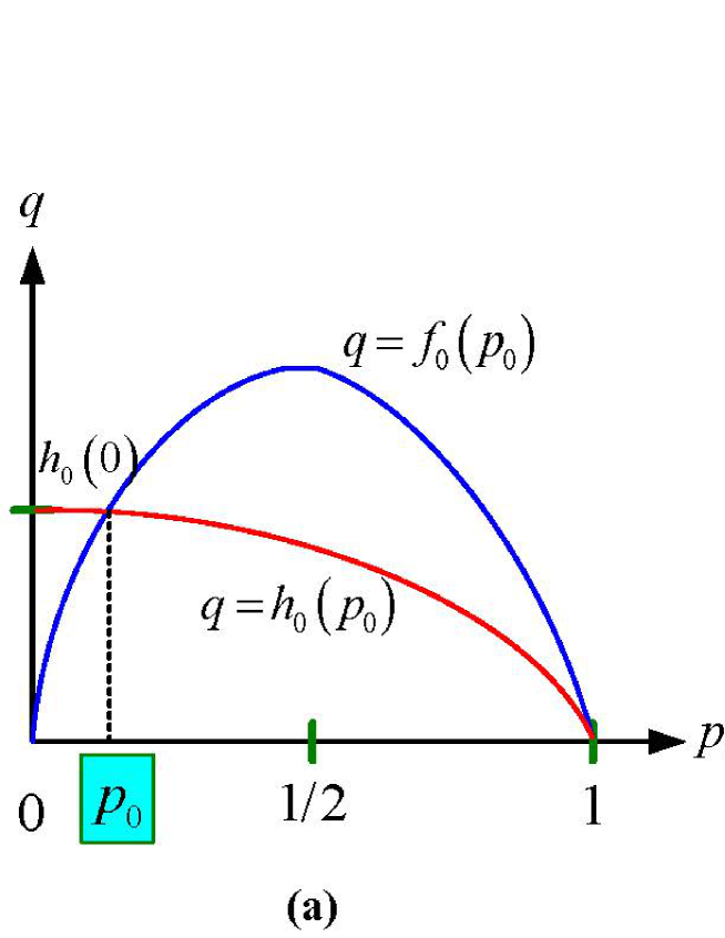
Figure 4: The uniqueness of the fixed point

Step two: Analyzing $p_{k}$ for $1\leq k\leq K-1$. In this case, we write

$$f_{k}\left(p_{k}\right)=\mu(1-p_{0})\left(C-\sum_{k=1}^{K}kp_{k}\right)(p_{k-1}-p_{k})$$

and

$$h_{k}\left(p_{k}\right)=\left[\lambda\left(1-p_{0}\right)+\gamma p_{0}\left(1-p_{0}^{\omega}\right)\right]\left(1-p_{K}\right)(p_{k}-p_{k+1}).$$

Note that

$$f_{k}\left(0\right)=\mu(1-p_{0})\left(C-\sum_{i\neq k}^{K}ip_{i}\right)p_{k-1}>0,$$

$$f_{k}\left(p_{k-1}\right)=0;$$

and for $0<p_{k}<p_{k-1}$

$$\frac{\text{d}}{\text{d}p_{k}}f_{k}\left(p_{k}\right)=\mu(1-p_{0})\left[-k(p_{k-1}-p_{k})-\left(C-\sum_{k=1}^{K}kp_{k}\right)\right]<0,$$

$$\frac{\text{d}^{2}}{\text{d}p_{k}^{2}}f_{k}\left(p_{k}\right)=2k\mu(1-p_{0})>0,$$

thus the quadratic function $f_{k}\left(p_{k}\right)$ is a strictly decreasing convex function for $0<p_{k}<p_{k-1}$.

Now, we consider the linear function $h_{k}\left(p_{k}\right)$. We obtain

$$h_{k}\left(0\right)=-\left[\lambda\left(1-p_{0}\right)+\gamma p_{0}\left(1-p_{0}^{\omega}\right)\right]\left(1-p_{K}\right)p_{k+1}<0,$$

and if $p_{k}=1$, then $p_{i}=0$ for $i\neq k$ with $1\leq i\leq K$, and it is clear that

$$h_{k}\left(1\right)=\lambda>0.$$

Since

$$\frac{\text{d}}{\text{d}p_{k}}h_{k}\left(p_{k}\right)=\left[\lambda\left(1-p_{0}\right)+\gamma p_{0}\left(1-p_{0}^{\omega}\right)\right]\left(1-p_{K}\right)>0,$$

the linear function $h_{k}\left(p_{k}\right)$ is strictly increasing for $p_{k}\in\left(0,1\right)$. Therefore, it is seen from Figure 4 (b) that there exists a unique solution $p_{k}$ to the equation $f_{k}\left(p_{k}\right)=h_{k}\left(p_{k}\right)$.

Step three: Analyzing $p_{K}$. Since $p_{k}$ is the unique solution to the equation $f_{k}\left(p_{k}\right)=h_{k}\left(p_{k}\right)$ for $0\leq k\leq K-1$, it is clear that $p_{K}$ can uniquely determined by means of the relation that $p_{K}=1-\sum_{k=0}^{K-1}p_{k}$. This completes the proof.  

Now, we provide a simple discussion for the limiting interchangeability of the vector $\mathbf{y}^{\left(N\right)}(t)$ as $N\rightarrow\infty$ and $t\rightarrow+\infty$. Note that the limiting interchangeability is always necessary and useful in many practical applications when using the stationary probabilities of the limiting process $\left\{\mathbf{Y}(t):t\geq 0\right\}$ to give an effective approximation for performance analysis of the bike sharing system.

From $\left|\mathbb{S}_{\mathbf{p}}\right|=1$ by Theorem 5, it is easy to see that

$$\lim_{t\rightarrow+\infty}\lim_{N\rightarrow\infty}\mathbf{y}^{\left(N\right)}\left(t\right)=\lim_{t\rightarrow+\infty}\mathbf{y}\left(t\right)=\mathbf{P}$$

and

$$\lim_{N\rightarrow\infty}\lim_{t\rightarrow+\infty}\mathbf{y}^{\left(N\right)}\left(t\right)=\lim_{N\rightarrow\infty}\mathbf{P}^{\left(N\right)}=\mathbf{P}.$$

This gives

$$\lim_{t\rightarrow+\infty}\lim_{N\rightarrow\infty}\mathbf{y}^{\left(N\right)}(t)=\lim_{N\rightarrow\infty}\lim_{t\rightarrow+\infty}\mathbf{y}^{\left(N\right)}(t)=\mathbf{p}.$$

Therefore, we have

$$\lim_{\begin{subarray}{c}N\rightarrow\infty\\ t\rightarrow+\infty\end{subarray}}\mathbf{y}^{\left(N\right)}(t)=\mathbf{p}.$$

Finally, we provide a simple discussion on the asymptotic independence of this bike sharing system. To this end, the uniqueness of the fixed point given by $\left|\mathbb{S}_{\mathbf{p}}\right|=1$ of Theorem 5 plays a key role. Using Corollaries 3 and 4 of Benaim and Le Boudec [4], we obtain the asymptotic independence of the queueing processes of the bike sharing system as follows:

$$\lim_{t\rightarrow+\infty}\lim_{N\rightarrow\infty}P\left\{X_{1}^{\left(N\right)}\left(t\right)=i_{1},X_{2}^{\left(N\right)}\left(t\right)=i_{2},\ldots,X_{k}^{\left(N\right)}\left(t\right)=i_{k}\right\}$$

$$=\lim_{N\rightarrow\infty}\lim_{t\rightarrow+\infty}P\left\{X_{1}^{\left(N\right)}\left(t\right)=i_{1},X_{2}^{\left(N\right)}\left(t\right)=i_{2},\ldots,X_{k}^{\left(N\right)}\left(t\right)=i_{k}\right\}$$

$$=p_{i_{1}}p_{i_{2}}\cdots p_{i_{k}}$$

and

$$\lim_{N\rightarrow\infty}\lim_{t\rightarrow+\infty}\frac{1}{t}\int_{0}^{t}\mathbf{1}_{\left\{X_{1}^{\left(N\right)}\left(t\right)=i_{1},X_{2}^{\left(N\right)}\left(t\right)=i_{2},\ldots,X_{k}^{\left(N\right)}\left(t\right)=i_{k}\right\}}\text{d}t$$

$$=\lim_{t\rightarrow+\infty}\lim_{N\rightarrow\infty}\frac{1}{t}\int_{0}^{t}\mathbf{1}_{\left\{X_{1}^{\left(N\right)}\left(t\right)=i_{1},X_{2}^{\left(N\right)}\left(t\right)=i_{2},\ldots,X_{k}^{\left(N\right)}\left(t\right)=i_{k}\right\}}\text{d}t$$

$$=p_{i_{1}}p_{i_{2}}\cdots p_{i_{k}}\text{ \ \ a.s.}$$

Remark 7

For a more complicated bike sharing system, it is possible to have $\left|\mathbb{S}_{\mathbf{p}}\right|\geq 2$. For this case with $\left|\mathbb{S}_{\mathbf{p}}\right|\geq 2$, the metastability of the bike sharing system is a key, and it can be roughly described as an interesting phenomenon which occurs when the bike sharing system stays a very long time in some abnormal state before reaching its normal state. To study the metastability, a useful method is to determine a Lyapunov function $g\left(\mathbf{y}\right)$ for the system of differential equations (such as, (6) and (7)). Therefore, we need to find a continuously differentiable, bounded from below, function $g\left(\mathbf{y}\right)$ defined on $\left[0,1\right]^{K+1}$ such that

$$\mathbf{yV}_{\mathbf{y}}\nabla g\left(\mathbf{y}\right)\leq 0.$$

Note that $\mathbf{yV}_{\mathbf{y}}\nabla g\left(\mathbf{y}\right)=0$ if $\mathbf{yV}_{\mathbf{y}}=0$, which is satisfied by $\mathbf{y=p}$. On the other hand, some properties of the function $g\left(\mathbf{y}\right)$ allow one to discriminate the stable points (the local minima of $g\left(\mathbf{y}\right)$) from the unstable points (the local maxima or saddle points of $g\left(\mathbf{y}\right)$) in the study of metastability.

In general, it is not easy to give an analytic solution to the system of nonlinear equations (21), but its numerical solution may always be simple and available. In the rest of this paper, we shall develop such a numerical solution, and give numerical computation for performance measures of this bike sharing system including the steady-state probability of the problematic stations, and the stationary expected number of bikes at the tagged station.

7 Numerical Analysis

In this section, we use some numerical examples to investigate the steady-state probability of the problematic stations. Based on this, performance analysis of the bike sharing system will focus on five points: (1) $p_{0}$; (2) $p_{K}$; (3) $p_{0}+p_{K}$; (4) $E\left[Q\right]=\sum_{k=1}^{K}kp_{k}$; and (5) the profit $R$.

Note that

$$\left\{\begin{array}[c]{c}\mathbf{pV}_{\mathbf{p}}=0,\\ \mathbf{p}e=1,\end{array}\right.$$

this gives the system of nonlinear equations (32) to (35) whose solution is unique by means of $\left|\mathbb{S}_{\mathbf{p}}\right|=1$ by Theorem 5. Also, we can numerically compute the unique solution, i.e., the fixed point $\mathbf{p}$. Furthermore, the fixed point $\mathbf{p}$ is employed in numerical computation for performance measures of the bike sharing system. Based on this, we use some numerical examples to give valuable observation and understanding with respect to design, operations and optimization of the bike sharing systems. Therefore, such a numerical analysis will become more and more useful in the study of bike sharing systems in practice.

7.1 Analysis of $p_{0}$

Note that $p_{0}$ is a probability that there is no bike in a tagged station, thus it is also the probability that the arriving customer can not rent a bike in the tagged station. To design a better bike sharing system, we hope that the value of $p_{0}$ is as small as possible, and this can be realized through taking a suitable parameters: $C,K,\lambda,\mu,\gamma$ and $\omega$, where $C,K\$and $\mu$ are controlled by the station; while $\lambda,\gamma$ and $\omega$ are given by the customers.

In this bike sharing system, we take that $C=30$, $K=50$, $\omega=1$ and $\gamma=0.25$. The left one of Figure 5 shows how the probability $p_{0}$ depends on $\lambda\in\left(10,30\right)$ when $\mu=0.3,1$ and $8$, respectively. It is seen that $p_{0}$ increases either as $\lambda$ increases or as $\mu$ decreases. Note that the numerical results are intuitively reasonable because what $\lambda$ increases quickens up the rental rate of bikes at the tagged station, while what $\mu$ decreases reduces the return rate of bikes at the tagged station. Hence the probability $p_{0}$ increases as the number of bikes parked at the tagged station decreases for the two cases.

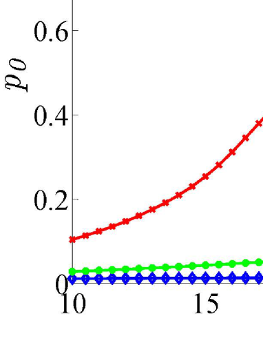
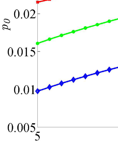
Figure 5: $p_{0}$ vs. $\lambda$, $\mu$ and $\gamma$

For the bike sharing system, we take that $C=30$, $K=50$, $\omega=1$ and $\mu=4$. The right one of Figure 5 indicates how the probability $p_{0}$ depends on $\lambda\in\left(5,15\right)$ when $\gamma=0.05,0.5$ and $1$, respectively. It is seen that $p_{0}$ increases as $\lambda$ increases or as $\gamma$ decreases.

7.2 Analysis of $p_{K}$

Different from $p_{0}$ given in Subsection 7.1, $p_{K}$ is a probability that the bikes are full in a tagged station, thus $p_{K}$ is also the probability that the bike-riding customer can not return his bike at the tagged station. To design a better bike sharing system, we hope that the value of $p_{K}$ is as small as possible through taking a suitable parameters: $C,K,\lambda,\mu,\gamma$ and $\omega$.

In this bike sharing system, we take that $C=30$, $K=50$, $\omega=1$ and $\gamma=0.25$. The left one of Figure 6 shows how the probability $p_{K}$ depends on $\lambda\in\left(10,30\right)$ when $\mu=4,8$ and $12$, respectively. It is seen that $p_{K}$ decreases either as $\lambda$ increases or as $\mu$ decreases. Note that what $\lambda$ increases speeds up the rental rate of bikes at the tagged station, while what $\mu$ decreases reduces the return rate of bikes at the tagged station.

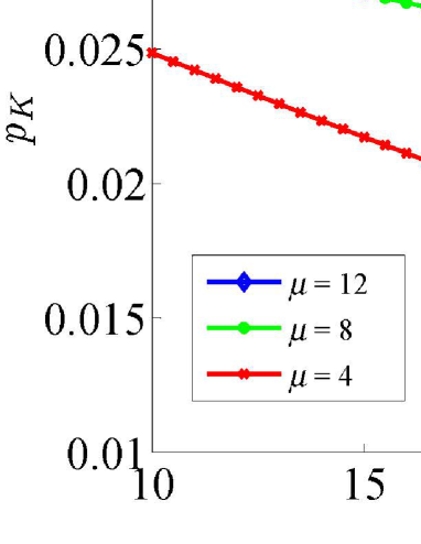
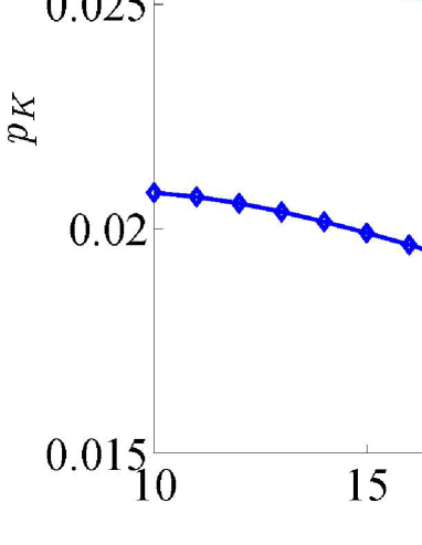
Figure 6: $p_{K}$ vs. $\lambda$, $\mu$ and $\gamma$

For the bike sharing system, we take that $C=30$, $K=50$, $\omega=1$ and $\mu=7$. The right one of Figure 6 indicates how the probability $p_{K}$ depends on $\lambda\in\left(10,30\right)$ when $\gamma=0.05,0.5$ and $3$, respectively. It is seen that $p_{K}$ decreases as $\lambda$ increases or as $\gamma$ increases.

7.3 Analysis of $p_{0}+p_{K}$

Based on the above two analysis for $p_{0}$ and $p_{K}$, we further hope that the value of $p_{0}+p_{K}$ can be as small as possible through taking a suitable parameters: $C,K,\lambda,\mu,\gamma$ and $\omega$.

In this bike sharing system, we take that $C=30$, $K=50$, $\omega=1$ and $\gamma=0.25$. The left one of Figure 7 shows how the probability $p_{0}+p_{K}$ depends on $\lambda\in\left(10,30\right)$ when $\mu=6,8$ and $10$, respectively. It is seen that $p_{0}+p_{K}$ decreases either as $\lambda$ increases or as $\mu$ decreases. Comparing Figure 7 with Figures 5 and 6, it is seen that $p_{K}$ has a bigger influence on the probability $p_{0}+p_{K}$ than $p_{0}$.

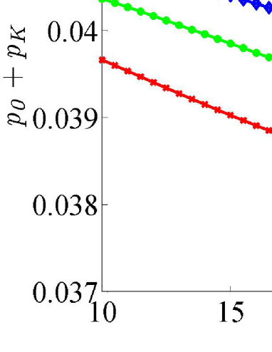
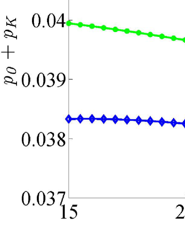
Figure 7: $p_{0}+p_{K}$ vs. $\lambda$, $\mu$ and $\gamma$

For the bike sharing system, we take that $C=30$, $K=50$, $\omega=1$ and $\mu=12$. The right one of Figure 7 indicates how the probability $p_{0}+p_{K}$ depends on $\lambda\in\left(15,30\right)$ when $\gamma=0.05,0.5$ and $1$, respectively. It is seen that $p_{0}+p_{K}$ decreases as $\lambda$ increases or as $\gamma$ increases.

7.4 Analysis of $E\left[Q\right]$

From $E\left[Q\right]=\sum_{k=1}^{K}kp_{k}$, it is seen that $E\left[Q\right]$ is the stationary expected number of bikes parked at the tagged station. Obviously, a customer who is renting a bike likes a bigger $E\left[Q\right]$, while a customer who is returning a bike likes a smaller $E\left[Q\right]$. In addition, $E\left[Q\right]$ can also be used to express the profit of the tagged station as follows:

$$R=-cE\left[Q\right]+\psi\left\{C-E\left[Q\right]\right\},$$

where $c$ is the cost price per bike and per time unit when a bike is parked in the tagged station, and $\psi$ is the benefit price per bike and per time unit when a bike is rented from the tagged station.

In this bike sharing system, we take that $C=30$, $K=50$, $\omega=1$ and $\gamma=0.25$. The left of Figure 8 shows how the stationary mean $E\left[Q\right]$ depends on $\lambda\in\left(10,30\right)$ when $\mu=2$, $5$ and $8$, respectively. It is seen that $E\left[Q\right]$ decreases either as $\lambda$ increases or as $\mu$ decreases.

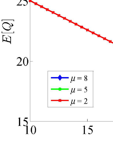
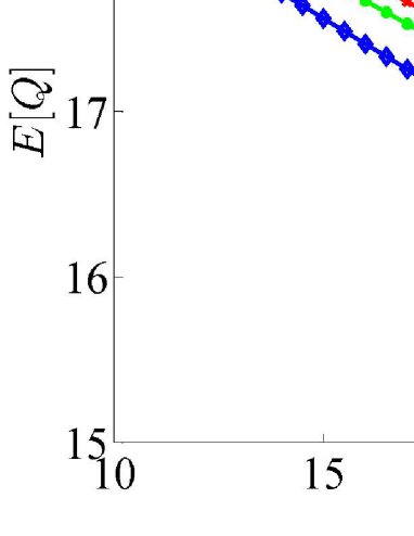
Figure 8: $E\left[Q\right]$ vs. $\lambda$, $\mu$ and $\gamma$

For the bike sharing system, we take that $C=20$, $K=50$, $\omega=1$ and $\mu=7$. The right of Figure 8 indicates how the stationary mean $E\left[Q\right]$ depends on $\lambda\in\left(10,30\right)$ when $\gamma=0.05$, $0.1$ and $6$, respectively. It is seen that $E\left[Q\right]$ decreases as $\lambda$ increases or as $\gamma$ increases.

7.5 Parameter optimization

We provide a simple discussion for how to optimize some key parameters of the bike sharing system through numerical experiments. Note that $\lambda$, $\gamma$ and $\omega$ are the arrival and walk information of any customer respectively, thus our parameter optimization will not consider them. In this case, our decision variables in the following optimal problems will mainly focus on the three parameters: $C$, $K$ and $\mu$.

(a) Optimization based on the probabilities $p_{0}$ and $p_{K}$

Since our purpose is to minimize either $p_{0}$, $p_{K}$ or $p_{0}+p_{K}$, we may choose a weighted method in which $\beta_{1},\beta_{2}$ and $\beta_{3}$ are the weighted coefficients with $\beta_{1},\beta_{2},\beta_{3}\geq 0$ and $\beta_{1}+\beta_{2}+\beta_{3}=1$. In this case, our optimal problem is given by

$$\min\left\{\beta_{1}p_{0}+\beta_{2}p_{K}+\beta_{3}\left(p_{0}+p_{K}\right)\right\}$$

s.t. $$0<\gamma<\mu,$$

$$1\leq C\leq K.$$

For example, when $\beta_{2}=0$ and $\beta_{3}=0$, $\min\left\{\beta_{1}p_{0}+\beta_{2}p_{K}+\beta_{3}\left(p_{0}+p_{K}\right)\right\}=\min\left\{p_{0}\right\}$; when $\beta_{1}=0$ and $\beta_{3}=0$, $\min\left\{\beta_{1}p_{0}+\beta_{2}p_{K}+\beta_{3}\left(p_{0}+p_{K}\right)\right\}=\min\left\{p_{K}\right\}$; when $\beta_{1}=0$ and $\beta_{2}=0$, $\min\left\{\beta_{1}p_{0}+\beta_{2}p_{K}+\beta_{3}\left(p_{0}+p_{K}\right)\right\}=\min\left\{p_{0}+p_{K}\right\}$. Therefore, our above optimal problem is a more general tradeoff among three key factors: $p_{0}$, $p_{K}$ and $p_{0}+p_{K}$.

(b) Optimization based on the profit $R$

Now, our optimal purpose is to maximize the profit of the tagged station as follows:

$$\max\left\{-cE\left[Q\right]+\psi\left\{C-E\left[Q\right]\right\}\right\}$$

s.t. $$0<\gamma<\mu,$$

$$1\leq C\leq K.$$

8 Concluding Remarks

In this paper, we apply the mean-field theory to studying a large-scale bike sharing system, where the mean-field computation can partly overcome the difficulty of state space explosion in more complicated bike sharing systems. We first use an $N$-dimensional Markov process to express the states of the bike sharing system, and construct an empirical measure Markov process of the $N$-dimensional Markov process. Then we set up the system of mean-field equations by means of a virtual time-inhomogeneous $M(t)/M(t)/1/K$ queue whose arrival and service rates are determined through some mean-field computation. Furthermore, we employ the martingale limit to investigate the limiting behavior of the empirical measure process, and prove that the fixed point is unique. This illustrates the asymptotic independence of the bike sharing system. Based on this, we can compute the fixed point through a nonlinear birth-death process, and provide some effective algorithms for computing the steady-state probability of the problematic stations. Finally, we use some numerical examples to give valuable observation on how the steady-state probability of the problematic stations depends on some crucial parameters of the bike sharing system.

This paper provides a complete picture on how to use the mean-field theory, the time-inhomogeneous queues, the martingale limits and the nonlinear Markov processes to analyze performance measures of the large-scale bike sharing systems. This picture is described as the following four key steps: (1) Setting up system of mean-field equations, (2) proofs of the mean-field limit, (3) uniqueness and computation of the fixed point, and (4) performance analysis of the bike sharing system. Therefore, the methodology and results of this paper give new highlight on understanding influence of system key parameters on performance measures of the bike sharing systems. Along such a line, there are a number of interesting directions for potential future research, for example:

• Analyzing impact of the intelligent information technologies on operations management of the bike sharing systems;

• discussing the bike sharing systems with non-exponential distributions and non-Poisson point processes, and develop some more general mean-field models;

• studying the periodical or time-inhomogeneous bike sharing systems; and

• modeling a bike sharing system with multiple clusters, where the unbalanced bikes can be redistributed among the stations or clusters by means of optimal scheduling of trucks.

References

- [1] Adelman D. Price-directed control of a closed logistics queueing network. Operation Research 2007;55(6):1022–1038.
- [2] Antunes N, Fricker C, Robert P, Tibi D. Stochastic networks with multiple stable points. The Annals of Probability 2008;36(1):255–278.
- [3] Barth M, Todd M. Simulation model performance analysis of a multiple station shared vehicle system. Transportation Research Part C: Emerging Technologies 1999;7(4):237–259.
- [4] Benaim M, Le Boudec JY. A class of mean-field interaction models for computer and communication systems. Performance Evaluation 2008;65(11–12):823–838.
- [5] Benchimol M, Benchimol P, Chappert B, Taille ADL, Laroche F, Meunier F, Robinet L. Balancing the stations of a self service “bike hire” system. Rairo-Operations Research 2011;45(1):37–61.
- [6] Billingsley P. Convergence of Probability Measures. Second Edition. John Wiley & Sons: New York; 1999.
- [7] Bordenave C, McDonald DR, Proutiere A. A particle system in interaction with a rapidly varying environment: mean-field limits and applications. Networks and Heterogeneous Media 2010;5(1):31–62.
- [8] Borgnat P, Robardet C, Rouquier JB, Abry P, Fleury E, Flandrin P. Shared bicycles in a city: A signal processing and data analysis perspective. Advances in Complex Systems 2011;14(3):415–438.
- [9] Bovier A. Markov Processes and Metastability. Lecture notes TUB; 2003.
- [10] Caggiani L, Ottomanelli M. A modular soft computing based method for vehicles repositioning in bike-sharing systems. Social and Behavioral Sciences 2012;54:675–684.
- [11] Chemla D, Meunier F, Calvo RW. Bike sharing systems: Solving the static rebalancing problem. Discrete Optimization 2013;14(3):120–146.
- [12] Côme E, Randriamanamihaga A, Oukhellou L, Aknin P. Spatio-temporal analysis of dynamic origin-destination data using latent Dirichlet allocation. Technical Report, Application to the Vélib’ Bike Sharing System of Paris, Université Paris-Est, IFSTTAR, COSYS-GRETTIA, F-77447 Marne-la-Vallée, France; 2013.
- [13] Contardo C, Morency C, Rousseau LM. Balancing a dynamic public bike-sharing system. Technical Report, CIRRELT; 2012.
- [14] Dawson DA. Critical dynamics and fluctuations for a mean-field model of cooperative behavior. Journal of Statistical Physics 1983;31(1):29–85.
- [15] Dell’Olio L, Ibeas A, Moura JL. Implementing bike-sharing systems. Proceedings of the ICE–Municipal Engineer 2011;164(2):89–101.
- [16] DeMaio P. Smart bikes: Public transportation for the 21st century. Transportation Quarterly 2003;57(1):9–11.
- [17] DeMaio P, Gifford J. Will smart bikes succeed as public transportation in the United States? Journal of Public Transportation 2004;7(2):1–15.
- [18] DeMaio P. Bike-sharing: history, impacts, models of provision, and future. Journal of Public Transportation 2009;12(4):41–56.
- [19] Den Hollander F. Metastability under stochastic dynamics. Stochastic Processes and their Applications 2004;114(1):1–26.
- [20] Ethier SN, Kurtz TG. Markov Processes: Characterization and Convergence. John Wiley & Sons; 1986.
- [21] Faye V. French network of bike: Cities and bikesharing systems in France. le Club des Villes Cyclables, Paris; 2008.
- [22] Forma I, Raviv T, Tzur M. The static repositioning problemin a bike-sharing system. In: Proceeding of the 7th Triennial Symposium on Transportation Analysis (TRISTAN), Tromsø Norway; 2010.
- [23] Fricker C, Gast N. Incentives and redistribution in homogeneous bike-sharing systems with stations of finite capacity. EURO Journal on Transportation and Logistics 2016;5(3):261–291.
- [24] Fricker C, Gast N, Mohamed A. Mean field analysis for inhomogeneous bikesharing systems. In: International Meeting on Probabilistic, Combinatorial and Asymptotic Methods for the Analysis of Algorithms; 2012.
- [25] Fricker C, Tibi D. Equivalence of ensembles for large vehicle-sharing models. arXiv preprint arXiv:1507.07792; 2015.
- [26] Froehlich J, Oliver N. Measuring the pulse of the city through shared bicycle programs. In: Proceedings of International Workshop on Urban, Community, and Social Applications of Networked Sensing Systems; 2008.
- [27] Gast N, Gaujal B. A mean field model of work stealing in large-scale systems. ACM SIGMETRICS Performance Evaluation Review 2010;38(1):13–24.
- [28] Gast N, Gaujal B. A mean field approach for optimization in discrete time. Discrete Event Dynamic Systems 2011;21(1):63–101.
- [29] Graham C. Chaoticity on path space for a queueing network with selection of the shortest queue among several. Journal of Applied Probabability 2000;37(1):198–201.
- [30] Graham C. Functional central limit theorems for a large network in which customers join the shortest of several queues. Probability Theory Related Fields 2004;131(1):97–120.
- [31] George DK, Xia CH. Asymptotic analysis of closed queueing networks and its implications to achievable service levels. SIGMETRICS Performance Evaluation Review 2010;38(2):3–5.
- [32] George DK, Xia CH. Fleet-sizing and service availability for a vehicle rental system via closed queueing networks. European Journal of Operational Research 2011;211(1):198–207.
- [33] Godfrey GA, Powell WB. An adaptive dynamic programming algorithm for dynamic fleet management, I: Single period travel times. Transportation Science 2002;36(1):21–39.
- [34] Guerriero F, Miglionico G, Olivito F. Revenue management policies for the truck rental industry. Transportation Research Part E 2012;48(1):202–214.
- [35] Hale JK. Ordinary Differential Equations. Roberte E. Krieger Publishing, Melbourne; 1980.
- [36] Janett B, Hendrik M. Optimising bike sharing in European cities: A handbook. OBIS Project; 2011.
- [37] Katzev R. Car sharing: A new approach to urban transportation problems. Analyses of Social Issues and Public Policy 2003;3(1):65–86.
- [38] Kumar VP, Bierlaire M. Optimizing locations for a vehicle sharing system. In: The Swiss Transport Research Conference; 2012.
- [39] Labadi K, Benarbia T, Barbot JP, Hamaci S, Omari A. Stochastic Petri net modeling, simulation and analysis of public bicycle sharing systems. IEEE Transactions on Automation Science and Engineering 2015;12(4):1380–1395.
- [40] Lathia N, Ahmed S, Capra L. Measuring the impact of opening the London shared bicycle scheme to casual users. Transportation Research Part C 2012;22(1):88–102.
- [41] Leurent F. Modelling a vehicle-sharing station as a dual waiting system: stochastic framework and stationary analysis. HAL Id: hal-00757228; 2012.
- [42] Li QL. Constructive Computation in Stochastic Models with Applications: The RG-Factorizations. Springer; 2010.
- [43] Li QL. Tail probabilities in queueing processes. Asia-Pacific Journal of Operational Research 2014;31(2):1–31.
- [44] Li QL. Nonlinear Markov processes in big networks. Special Matrices 2016;4:202–217.
- [45] Li QL, Dai GR, Lui JCS, Wang Y. The mean-field computation in a supermarket model with server multiple vacations. Discrete Event Dynamic Systems 2014;24(4):473–522.
- [46] Li QL, Du Y, Dai GR, Wang M. On a doubly dynamically controlled supermarket model with impatient customers. Computers & Operations Research 2015;55:76–87.
- [47] Li QL, Fan RN. Bike-sharing systems under Markovian environment. arXiv preprint arXiv:1610.01302; 2016.
- [48] Li QL, Fan RN, Ma JY. A unified framework for analyzing closed queueing networks in bike sharing systems. In: International Conference on Information Technologies and Mathematical Modelling. Springer; 2016.
- [49] Li QL, Lui J.C.S. Block-structured supermarket models. Discrete Event Dynamic Systems 2016;26(2):147–182.
- [50] Lin JR, Yang TH. Strategic design of public bicycle sharing systems with service level constraints. Transportation Research Part E 2011;47(2):284–294.
- [51] Lin JR, Yang TH, Chang YC. A hub location inventory model for bicycle sharing system design: Formulation and solution. Computers & Industrial Engineering 2013;65(1):77–86.
- [52] Liu Z, Jia X, Cheng W. Solving the last mile problem: Ensure the success of public bicycle system in Beijing. Social and Behavioral Sciences 2012;43(1):73–78.
- [53] Martin JB, Suhov YM. Fast Jackson networks. The Annals of Applied Probability 1999;9(3):854–870.
- [54] Martinez LM, Caetano L, Eiró T, Cruz F. An optimisation algorithm to establish the location of stations of a mixed fleet biking system: An application to the city of Lisbon. Social and Behavioral Sciences 2012;54(4):513–524.
- [55] Meddin R, DeMaio P. The bike sharing world map. URL http://www.metrobike.net; 2012.
- [56] Mitzenmacher MD. The power of two choices in randomized load balancing. PhD thesis, Department of Computer Science, University of California at Berkeley, USA; 1996.
- [57] Morency C, Trépanier M, Godefroy F. Insight into the Montreal bikesharing system. In: TRB-Transportation Research Board Annual Meeting, Washington, USA; 2011.
- [58] Nair R, Miller-Hooks E. Fleet management for vehicle sharing operations. Transportation Science 2011;45(4):524–540.
- [59] Nair R, Miller-Hooks E, Hampshire RC, Bušic A. Large-scale vehicle sharing systems: Analysis of vélib’. International Journal of Sustainable Transportation 2013;7(1):85–106.
- [60] Raviv T, Kolka O. Optimal inventory management of a bike-sharing station. IIE Transactions 2013;45(10):1077–1093.
- [61] Raviv T, Tzur M, Forma IA. Static repositioning in a bike-sharing system: models and solution approaches. EURO Journal on Transportation and Logistics 2013;2(3):187–229.
- [62] Rogers LCG, Williams D. Diffusions, Markov Processes, and Martingales, Vol. 1: Foundations. John Wiley & Sons: New York; 1994.
- [63] Savin S, Cohen M, Gans N, Katala Z. Capacity management in rental businesses with two customer bases. Operations Research 2005;53(4):617–631.
- [64] Shaheen SA, Guzman SY. Worldwide bikesharing. Access 2011;39:22–27.
- [65] Shaheen SA, Guzman SY, Zhang H. Bike sharing in Europe, the American and Asia: Past, present and future. In: Transportation Research Board 89th Annual Meeting, Washington, D.C.; 2010.
- [66] Schuijbroek J, Hampshire R, van Hoeve WJ. Inventory rebalancing and vehicle routing in bike sharing systems. Technical Report-1491, Tepper School of Business, Carnegie Mellon University; 2013.
- [67] Shu J, Chou MC, Liu Q, Teo CP, Wang IL. Models for effective deployment and redistribution of bicycles within public bicycle-sharing systems. Operations Research 2013;61(6):1346–1359.
- [68] Spitzer F. Interaction of Markov processes. Advances in Mathematics 1970;5(2):246–290.
- [69] Sznitman A. Topics in propagation of chaos. In: Springer-Verlag Lecture Notes in Mathematics 1464, École d’Été de Probabilités de Saint-Flour XI; 1989.
- [70] Tibi D. Metastability in communications networks. arXiv preprint arXiv:1002.07/96v1; 2010.
- [71] Turner SRE. The effect of increasing routing choice on resource pooling. Probability in the Engineering and Informational Sciences 1998;12(1):109–124.
- [72] Vogel P, Mattfeld DC. Modeling of repositioning activities in bike-sharing systems. In: Proceeding of the 12th World Conference on Transport Research; 2010.
- [73] Vogel P, Greiser T, Mattfeld DC. Understanding bike-sharing systems using data mining: Exploring activity patterns. Social and Behavioral Sciences 2011;20(6):514–523.
- [74] Vvedenskaya ND, Dobrushin RL, Karpelevich FI. Queueing system with selection of the shortest of two queues: An asymptotic approach. Problems of Information Transmissions 1996;32(1):15–27.
- [75] Waserhole A, Jost V. Vehicle sharing system pricing regulation: Transit optimization of intractable queuing network. Technical Report, INRIA; 2012.
- [76] Waserhole A, Jost V. Vehicle sharing system pricing regulation: A fluid approximation. HAL Id: hal-00727041; 2013.
- [77] Waserhole A, Jost V. Pricing in vehicle sharing systems: Optimization in queuing networks with product forms. EURO Journal on Transportation and Logistics 2016;5(3):293–320.
- [78] Waserhole A, Jost V, Brauner N. Pricing techniques for self regulation in vehicle sharing systems. Electronic Notes in Discrete Mathematics 2013;41:149–156.
- [79] Whitt W. Stochastic-Process Limits: An Introduction to Stochastic-Process Limits and Their Application to Queues. Springer; 2002.