Test for a universal behavior of Dirac eigenvalues in the complex Langevin method

Abstract

We apply the complex Langevin (CL) method to a chiral random matrix theory (ChRMT) at non-zero chemical potential and study the nearest neighbor spacing (NNS) distribution of the Dirac eigenvalues. The NNS distribution is extracted using an unfolding procedure for the Dirac eigenvalues obtained in the CL method. For large quark mass, we find that the NNS distribution obeys the Ginibre ensemble as expected. For small quark mass, the NNS distribution follows the Wigner surmise for correct convergence case, while it follows the Ginibre ensemble for wrong convergence case. The Wigner surmise is physically reasonable from the chemical potential independence of the ChRMT. The Ginibre ensemble is known to be favored in a phase quenched QCD at finite chemical potential. Our result suggests a possibility that the originally universal behavior of the NNS distribution is preserved even in the CL method for correct convergence case.

I Introduction

The complexification of field theories has attracted recent attention in the context of solving the sign problem. The complex Langevin (CL) method Parisi (1983); Klauder (1984); Seiler et al. (2013) and the Lefshetz thimble (LT) method Pham (1983); Witten (2011, 2010) rely on the complexification of dynamical variables of the system. Although they are hopeful candidates as a solution for the sign problem, there are still some controversies over their feasibility or practicality. One of the difficulties lies in the lack of knowledge of complexified theories, which we would like to address in this work.

The Langevin method is based on the stochastic quantization Parisi and Wu (1981). As for real actions, the Langevin method is ensured to produce correct results in an infinitely large Langevin-time limit, where the probability distribution of dynamical variables approaches to the Boltzmann weight as indicated in the eigenvalue analysis of the Fokker-Planck equation, e.g. see Refs. Namiki et al. (1992); Damgaard and Huffel (1987). As for complex actions Parisi (1983); Klauder (1984), observables in the CL method sometimes converge to wrong results. Recently, Aarts et al. showed that the CL method can be justified if some conditions are satisfied Aarts et al. (2010a, 2011). Possible reasons of its breakdown are the spread of CL configurations in the complexified direction in the complex plane of field variables Aarts et al. (2010a, 2011) and singular drift terms of CL equations Mollgaard and Splittorff (2013); Greensite (2014); Nishimura and Shimasaki (2015).

A new method, which is referred to as the gauge cooling, has been proposed to suppress the spread of configurations in the imaginary direction by using the complexified gauge invariance Seiler et al. (2013); Sexty (2014); Fodor et al. (2015). It was shown that the method reproduces correct results of physical observables in some cases Seiler et al. (2013). Later, the gauge cooling method is justified in Ref. Nagata et al. (2016), and extended to theories that have a global symmetry with sufficiently large number of generators Nagata et al. (2015). In addition, it was found in Ref. Mollgaard and Splittorff (2013) that the singular drift problem occurred in a chiral random matrix theory (ChRMT), where complex eigenvalues of the fermion matrix touch the origin at non-zero chemical potential. Here the fermion matrix is given as $D+m$ with a Dirac operator $D$. Zero modes of the fermion matrix cause a singularity in a drift term of the Langevin equation. Such a singularity originates from the logarithmic term in the effective action, which is expected to occur for fermionic theories quite in general. Mollgaard and Splittorff pointed out that a suitable parameterization of dynamical variables solves this problem in the ChRMT Mollgaard and Splittorff (2015). They showed that the fermion matrix eigenvalues are well localized, deviating from the origin, and the simulation converges to the correct result. It was also shown in Ref. Nagata et al. (2015) that the gauge cooling can be extended to the singular drift problem by using suitable norms.

With regard to the convergence problem, it is interesting to focus on universal quantities to understand if the CL method converges correctly. The CL method can reproduce correct results of the universal quantities that are defined as holomorphic quantities if the conditions for justification are satisfied Aarts et al. (2010a, 2011). On the other hand, it is unclear if the CL method can reproduce physical results for non-holomorphic quantities. However, it may be natural to expect that the original universality is preserved for the correct convergence cases as in one classical thimble calculation in the LT method Cristoforetti et al. (2012).

The nearest neighbor spacing (NNS) distribution is one of the universal quantities which reflect the correlations of the fermion matrix eigenvalues and the property of the matrix. The NNS distribution has been investigated in the phase quenched QCD at zero and non-zero chemical potential by using MC simulations Markum et al. (1999). They showed that the NNS distribution obeys some kinds of distributions: the Ginibre, Wigner, and Poisson distributions, depending on the system and the strength of the eigenvalue correlations. We note that the NNS distribution is obtained from the density of the fermion matrix eigenvalues and it is not a holomorphic quantity Stephanov (1996). This fact implies that the distribution obtained in the CL method does not necessarily reproduce the NNS distribution in the original theory Nagata et al. (2015). However, the Dirac eigenvalues are closely related to the convergence property of the CL method, and the NNS distribution is a universal quantity obtained from Dirac eigenvalues. Therefore, it can be valuable to investigate the universal behavior of the NNS distribution of the Dirac eigenvalues in the CL method deeply to understand the complexified theory.

We conjecture that the NNS distribution can reproduce physical results in the CL method even though it is non-holomorphic. This conjecture may be natural if the NNS distribution reflects the properties of the critical points (or saddle points) owing to its universality. Since the Dirac eigenvalues can depend on the choice of the convergence properties of the CL method Mollgaard and Splittorff (2015), then at least we can expect that the convergence property of the CL method also affect the NNS distribution. In the CL simulations, configurations fluctuate around a classical flow and locate around some critical points. The different convergence properties indicate that the configurations locate around different critical points. Then, we expect that the underlying universality at each critical point can be different in the two cases with the correct and wrong convergences in ChRMT Mollgaard and Splittorff (2013, 2015).

In this work, we investigate the NNS distributions of the ChRMT in the CL method, where we employ two parameterizations based on Refs. Mollgaard and Splittorff (2013, 2015): one leads to correct convergence and the other leads to wrong one. Our purposes are following: (I) analyzing what happens in the wrong and correct convergent cases in the NNS distribution and (II) comparing the CL result with the previous MC expectations for the NNS distribution.

This paper is organized as follows. In the next section, we define the ChRMT and introduce the two parameterizations. In Sec. II, we introduce the CL method. We also explain the procedure for calculating the NNS distribution with complex eigenvalues Markum et al. (1999) in Sec. III. In Sec. IV, we give results on the NNS distribution and discussions of them. Sec. V is devoted to a summary.

II Chiral Random Matrix Theory

II.1 Two types of representations

In this work, we study the ChRMT introduced in Ref. Osborn (2004) in two types of the representation: first one is used in Ref. Mollgaard and Splittorff (2013), and the second one is used in Ref. Mollgaard and Splittorff (2015). Those two representations are equivalent under the linear transformation of dynamical variables before complexification Bloch et al. (2013). In both cases, we describe originally complex dynamical variables in the polar coordinate.

Throughout this work, we consider only the case of zero topological-index and of two flavor $N_{f}=2$. The partition function of the ChRMT is given as

$$Z =\int d\Phi_{1}d\Phi_{2}(\det(D+m))^{N_{f}}e^{-N\operatorname{\mathrm{Tr}\,}(\Phi_{1}^{\dagger}\Phi_{1}+\Phi_{2}^{\dagger}\Phi_{2})}$$

$$=\int d\Phi_{1}d\Phi_{2}\exp(-S)\ .$$ (1)

$\Phi_{1,2}$ are $N\times N$ complex matrices.

Representation (I): Hyperbolic type

First, we consider the following case, where the action and the Dirac operator are

$$S=N\mathrm{Tr}[\Phi_{1}^{\dagger}\Phi_{1}+\Phi_{2}^{\dagger}\Phi_{2}]-N_{f}\mathrm{Tr}\log(G^{-1})\ ,$$ (2)

$$D(\mu)+m=\left(\begin{matrix}0&X\\ Y&0\end{matrix}\right)+m\ ,$$ (3)

here $G^{-1}=m^{2}-XY$. The $X$ and $Y$ are complex $N\times N$ matrices,

$$X \equiv i\cosh(\mu)\Phi_{1}+\sinh(\mu)\Phi_{2}^{\dagger}\ ,$$ (4)

$$Y \equiv i\cosh(\mu)\Phi_{1}^{\dagger}+\sinh(\mu)\Phi_{2}\ .$$ (5)

We call this parameterization hyperbolic (Hyp) representation below. Here, elements of the random matrices, $\Phi_{1}$ and $\Phi_{2}$, are originally complex, and can be parameterized in terms of two real variables. In the present study, we employ the polar coordinate Mollgaard and Splittorff (2015), where

$$\left(\Phi_{1}\right)_{ij}=r_{1,ij}e^{i\theta_{1,ij}}\ \ ,\ \left(\Phi_{2}\right)_{ij}=r_{2,ij}e^{i\theta_{2,ij}}\ ,$$ (6)

for $i,j=1,\cdots,N$. The matrices $X$ and $Y$ are given as

$$X_{ij} =i\cosh(\mu)r_{1,ij}e^{i\theta_{1,ij}}+\sinh(\mu)r_{2,ji}e^{-i\theta_{2,ji}}\ ,$$ (7)

$$Y_{ij} =i\cosh(\mu)r_{1,ji}e^{-i\theta_{1,ji}}+\sinh(\mu)r_{2,ij}e^{i\theta_{2,ij}}\ .$$ (8)

The action is rewritten as

$$S= -\sum_{i,j}\left(\log(r_{1,ij})+\log(r_{2,ij})\right)$$

$$-N_{f}\log\det(G^{-1})+N\sum_{i,j}\left(r_{1,ij}^{2}+r_{2,ji}^{2}\right)\ .$$ (9)

Representation (II): Exponential type

Next, we consider the other parameterization used in Ref. Mollgaard and Splittorff (2015) as

$$X\equiv e^{\mu}\Phi_{1}-e^{-\mu}\Phi_{2}^{\dagger}\ ,$$ (10)

$$Y\equiv -e^{-\mu}\Phi_{1}^{\dagger}+e^{\mu}\Phi_{2}\ .$$ (11)

The action is given by

$$S=2N{\rm Tr}[\Phi_{1}^{\dagger}\Phi_{1}+\Phi_{2}^{\dagger}\Phi_{2}]-N_{f}{\rm Tr}\log(G^{-1}).$$ (12)

This parameterization is referred to as Exponential (Exp) representation below. We also use the polar coordinate in this representation.

The two representations are equivalent under a linear transformation Bloch et al. (2013); Mollgaard and Splittorff (2015). Note that the CL method is applied to the ChRMT with the Hyp representation and with the Cartesian coordinate in Ref. Mollgaard and Splittorff (2013), while it is applied to the ChRMT with the Exp representation and with the polar coordinate in Ref. Mollgaard and Splittorff (2015). In this work, we adopt the polar coordinate both for the two representations. We will confirm that only the case of the Exp representation reproduces the correct results if the mass of quark is small at non-zero quark chemical potential.

II.2 Langevin equations and drift terms

Now, we apply the Langevin equation to the originally real variables in the system $\varphi_{k}\in\{r_{1,ij},r_{2,ij},\theta_{1,ij},\theta_{2,ij}|\,i,j=1,\cdots,N,(i,j\in\mathbb{Z})\}$.

$$\frac{\partial\varphi_{k}(\tau)}{\partial\tau}=-\frac{\partial S[\varphi]}{\partial\varphi_{k}}+\eta_{k}(\tau)\ ,$$ (13)

where $\tau$ is the Langevin time. The Gaussian noise, $\eta_{k}$, is normalized as $\left<\eta_{k}(\tau)\right>=0$ and $\left<\eta_{k}(\tau)\eta_{l}(\tau^{\prime})\right>=2\delta_{kl}\delta(\tau-\tau^{\prime})$. Since the action is complex at $\mu\neq 0$, those variables are extended to complex $r_{1},r_{2},\theta_{1},\theta_{2}\in\mathbb{R}\to\mathbb{C}$. In this paper, we use the real Gaussian noise $\eta_{k}\in\mathbb{R}$ and the adaptive step size method Ambjorn et al. (1986); Aarts et al. (2010b); Aarts and James (2010). We explicitly show the drift terms in the Hyp representation in Sec. A, and those in the Exp representation were shown in Ref. Mollgaard and Splittorff (2015).

In the numerical simulation, we define the discretized Langevin equation

$$\varphi_{k}(\tau+d\tau)=\varphi_{k}(\tau)+d\tau\biggl{(}-\frac{\partial S[\varphi]}{\partial\varphi_{k}}\biggr{)}+\sqrt{d\tau}\,\eta_{k}(\tau).$$ (14)

In the adaptive stepsize method in Ref. Aarts and James (2010), we can adopt an average value of a maximum drift term at each Langevin time before the thermalization time $\tau_{\rm th}$,

$$\left<\mathcal{K}_{\mathrm{max}}\right>_{\mathrm{th}}=\frac{1}{N_{\mathrm{th}}}\sum_{\tau^{\prime}=0}^{\tau_{\mathrm{th}}}\mathcal{K}_{\mathrm{max}}(\tau^{\prime})\ ,$$ (15)

where $\mathcal{K}_{\mathrm{max}}(\tau^{\prime})=\max_{k,\varphi=r_{1},r_{2},\theta_{1},\theta_{2}}\left|\varphi_{k}(\tau^{\prime})\right|$ and $N_{\mathrm{th}}=\tau_{\mathrm{th}}/d\tau$ is the number of configurations until the thermalization time, $\tau_{\mathrm{th}}$. After the thermalization time, we adopt an adaptive stepsize at each Langevin time as

$$\epsilon_{\tau}=\min(d\tau,d\tau\left<\mathcal{K}_{\mathrm{max}}\right>_{\mathrm{th}}/\mathcal{K}_{\mathrm{max}}(\tau))\ ,$$ (16)

and then the CL equation is given as

$$\varphi_{k}(\tau+\epsilon_{\tau})=\varphi_{k}(\tau)+\epsilon_{\tau}\left(-\frac{\partial S[\varphi]}{\partial\varphi_{k}}\right)+\sqrt{\epsilon_{\tau}}\eta_{k}(\tau)\ .$$ (17)

III Nearest Neighbor spacing distribution

In order to obtain the nearest neighbor spacing (NNS) distributions, we need a procedure so called unfolding. We follow the unfolding procedure introduced in Ref. Markum et al. (1999).

III.0.1 Unfolding procedure with complex eigenvalues

First, we define the density of Dirac eigenvalues as

$$\rho(x,y)=\left<\sum_{k}\delta^{(2)}(z-z_{k})\right>\ ,\,(z=x+iy)$$ (18)

where $\left<\cdots\right>$ denotes an ensemble average and $z_{k}$ is an eigenvalue of the Dirac operator $D(\mu)\ket{z_{k}}=z_{k}\ket{z_{k}},\,(k=1,\cdots 2N)$. Due to the property of the Dirac operator $\{\gamma_{5},D(\mu)\}=0$, the eigenvalues appear as $\pm z$ pair Akemann et al. (2005). The density of the Dirac eigenvalue $\rho(x,y)$ is non-holomorphic Stephanov (1996).

In order to obtain the fluctuation part of the eigenvalue density, we rewrite $\rho(x,y)$ as

$$\rho(x,y)=\rho_{\mathrm{ave}}(x,y)+\rho_{\mathrm{fluc}}(x,y)\ ,$$ (19)

where $\rho_{\mathrm{ave}}$ and $\rho_{\mathrm{fluc}}$ are the average part and the fluctuation part of the eigenvalue density, respectively. We consider a map

$$z^{\prime}=x^{\prime}+iy^{\prime}=u(x,y)+iv(x,y)\ ,$$ (20)

where we impose a condition that the average eigenvalue density is unity for any points on the new coordinate, namely $\rho_{\mathrm{ave}}(x^{\prime},y^{\prime})=1$. It immediately follows from the probability conservation condition that $\rho_{\mathrm{ave}}(x^{\prime},y^{\prime})dx^{\prime}dy^{\prime}=dx^{\prime}dy^{\prime}=\rho_{\mathrm{ave}}(x,y)dxdy$ Markum et al. (1999). On the other hand, it follows from Eq. (20) that $dx^{\prime}dy^{\prime}=Jdxdy,$ where $J=|\partial(x^{\prime},y^{\prime})/\partial(x,y)|$ is the Jacobian of the coordinate transformation. Combining the two relations implies that the $\rho_{\mathrm{ave}}(x,y)$ is nothing but the Jacobian, i.e.,

$$\rho_{\mathrm{ave}}(x,y)=\left|\partial_{x}u\partial_{y}v-\partial_{x}v\partial_{y}u\right|\ .$$ (21)

$u(x,y)$ and $v(x,y)$ are not determined uniquely only from this condition. We choose $y^{\prime}=v(x,y)=y$, which reduces Eq. (21) to $\rho_{\mathrm{ave}}(x,y)=\partial_{x}u$ Markum et al. (1999). The real part of eigenvalues is expressed as

$$x^{\prime}=u(x,y)=\int_{-\infty}^{x}dt\rho_{\mathrm{ave}}(t,y)\equiv N_{\mathrm{ave}}(x,y)\ ,$$ (22)

where $N_{\mathrm{ave}}(x,y)$ is the average part of the cumulative spectral function $N(x,y)$ Guhr et al. (1998), which is given as

$$N(x,y)=N_{\mathrm{ave}}(x,y)+N_{\mathrm{fluc}}(x,y)\ .$$ (23)

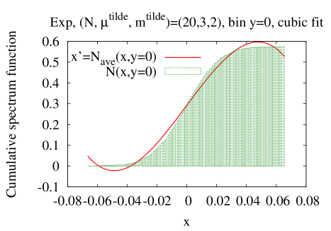
Figure 1: The cumulative spectral function $N(x,y)$ (histogram) and its average part $N_{\rm ave}(x,y)$ (solid line) as a function of $x$ at $N=20$, $\tilde{m}=2$, and $\tilde{\mu}=3$ in the Exp representation. They are obtained from eigenvalues included in a strip around $y=0$. The top and bottom panels are obtained with a cubic function and a quintic function, respectively.

In order to obtain the cumulative spectral function numerically, we first divide the complex plane in the $y$-direction, where each strip has a width $dy$. In the ChRMT, a spacing between two adjacent eigenvalues is of an order $\mathcal{O}(1/N)$ Verbaarschot and Wettig (2000). We choose the width $dy$ so that it is bigger than this magnitude: $dy=0.1$ at $N=20$, for example. If we adopt too small $dy$, there are few eigenvalues in a given strip. Then, we calculate $N(x,y)$ for each strip. In our calculations, we derive the average cumulative spectral function by fitting $N_{\mathrm{ave}}$ with a low order polynomial as in Ref. Markum et al. (1999). Then, we adopt a sufficiently small bin size for $x$ to fit $N_{\mathrm{ave}}$ appropriately. We use a quintic polynomial throughout this paper, but the validity of the fitting procedure is checked by comparing results with the quintic and cubic polynomials. In Fig. 1, we show $N_{\rm ave}(x,y)$ obtained from the cubic polynomial (top panel), and from the quintic polynomial (bottom panel). We find that the NNS distribution is quantitatively insensitive to the choice of the fitting functions, which will be shown in Appendix B.

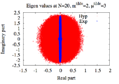
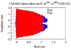
Figure 2: Dirac eigenvalues at $N=20$, $\tilde{m}=2$, and $\tilde{\mu}=3$ before unfolding procedure (left panel) and after unfolding procedure (right panel). They are obtained from configurations in late Langevin time.

To illustrate the unfolding procedure, we show Dirac eigenvalues at $N=20$, $\tilde{m}=2$, and $\tilde{\mu}=3$ obtained with various ensembles at late Langevin times in Fig. 2 where $\tilde{m}=Nm$ and $\tilde{\mu}=\sqrt{N}\mu$. As in Ref. Mollgaard and Splittorff (2015), the width of Dirac eigenvalues in the Exp representation decreases along the real axis compared with that in the Hyp representation. The right panel shows the Dirac eigenvalues after the unfolding. The unfolded distribution is apparently consistent with the distribution obtained in the phase quenched QCD Markum et al. (1999).

III.0.2 Nearest Neighbor spacing distribution with complex eigenvalues

In order to derive the NNS distribution from complex eigenvalues, we need to introduce the NNS, $s$. There is an ambiguity to define $s$ for the complex eigenvalues. We adopt $s_{i}(\tau)=\min_{j}\left|z_{i}^{\prime}-z_{j}^{\prime}\right|$ for $i=1,\cdots,2N$ using unfolded eigenvalues at Langevin time $\tau$ Markum et al. (1999). We construct the distribution $p(s)$ of $s_{i}(\tau)$ for $(i=1,\cdots,2N)$, where we use all the configurations in late Langevin time with a certain interval.

The NNS distribution $P(s)$ is defined so that it satisfies two conditions $\int dsP(s)=1$ and $\int dssP(s)=1$. In order to satisfy these conditions, we use the normalization and rescaling of $s$ Markum et al. (1999): supposing that the first moment of the distribution is $c=\int_{0}^{\infty}dssp(s)$ with $1=\int_{0}^{\infty}dsp(s)$, the new distribution is defined by $P(s)=cp(cs)$. Once the distribution satisfies the two conditions, we can compare the distribution obtained in the present work with some typical distributions.

III.0.3 Reference NNS distributions

Here, we explain three typical NNS distributions, which are used as references to understand numerical results obtained from CL simulations.

At $\mu=0$, the Dirac operator is anti-Hermitian, and its eigenvalues are pure imaginary. The NNS distribution in the chiral unitary ensemble of RMT follows the Wigner surmise Halasz and Verbaarschot (1995); Guhr et al. (1998); Markum et al. (1999)

$$P_{W}(s)=\frac{32}{\pi^{2}}s^{2}e^{-4s^{2}/\pi}.$$ (24)

It is expected that the NNS distribution in this work also follows the Wigner surmise. We will discuss the mass dependence in Sec. IV.

On the other hand, at $\mu\neq 0$, the Dirac operator is no more anti-Hermitian, and its eigenvalues are generally complex. If the real and imaginary part of eigenvalues have approximately the same average magnitude, then the system is described by the Ginibre ensemble Ginibre (1965) of non-Hermitian RMT Ginibre (1965); Markum et al. (1999). In this case, the NNS distribution is given by

$$P_{G}(s) =cp(cs),$$ (25)

$$p(s) =2s\lim_{N\to\infty}\left[\prod_{n=1}^{N-1}e_{n}(s^{2})e^{-s^{2}}\right]\sum_{n=1}^{N-1}\frac{s^{2n}}{n!e_{n}(s^{2})},$$ (26)

where $e_{n}(x)=\sum_{m=0}^{n}x^{m}/m!$ and $c=\int_{0}^{\infty}dssp(s)$ Grobe et al. (1988); Markum et al. (1999). In this paper, we use $N=2000$ in Eq. (26) as a reference distribution.

For uncorrelated eigenvalues, the NNS distribution follows the Poisson distribution. On the complex plane, the Poisson distribution is given by Grobe et al. (1988)

$$P_{P}(s)=\frac{\pi}{2}se^{-\pi s^{2}/4}.$$ (27)

IV Results and discussion

In this section, we show numerical results obtained from the CL simulations. Our numerical set up is as follows. We consider the ChRMT with zero topological index $\nu=0$, $N=20$ and $N_{f}=2$. We utilize the reference step size as $d\tau=1.0\times 10^{-6}$, and perform the simulation with the adaptive stepsize Aarts and James (2010). We take the Langevin time $\tau\sim 50$ for thermalization, and $\tau\sim 100$ for measurements. The measurement is performed by using configurations in late Langevin time, and the number of typical configurations for the measurement is 2000.

In the following, we show the numerical results for $\tilde{\mu}=1$ and $\tilde{\mu}=3$, where $\tilde{m}=Nm$ and $\tilde{\mu}=\sqrt{N}\mu$.

IV.1 Results for $N=20$ at $\tilde{\mu}=1$

In Fig. 3, we show the chiral condensate at $\tilde{\mu}=1$ as a function of $\tilde{m}$. Here the chiral condensate is given by Mollgaard and Splittorff (2013),

$$\frac{1}{N}\left<\bar{\eta}\eta\right> =\frac{1}{N}\left<\partial_{m}\log(Z)\right>$$

$$=\frac{2mN_{f}}{N}\left<\mathrm{Tr}\left[(m^{2}-XY)^{-1}\right]\right>\ .$$ (28)

There is a small difference between analytical results for the exact Osborn (2004) and phase quenched Akemann et al. (2005) cases for small $\tilde{m}$, which are denoted as “exact” and “PQ exact” in Fig. 3, respectively. Numerical results with the Exp representation and Hyp representation are almost consistent with analytical results for the exact and phase quenched cases.

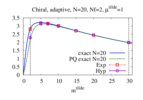
Figure 3: The chiral condensate at $\tilde{\mu}=1$ as a function of $\tilde{m}$. The solid line shows the exact value in the ChRMT Osborn (2004) and the dotted line shows the exact value in the phase quenched (PQ) ChRMT Akemann et al. (2005). The results of the Exp and Hyp representations are expressed as squares and circles. At large $\tilde{m}$, both representations well produce exact results. Results of the Hyp representation slightly deviate from exact results at small $\tilde{m}$. Dotted vertical lines show the values of $\tilde{m}$ at which the NNS distribution is obtained.

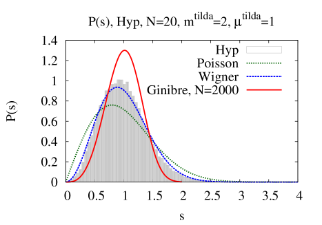
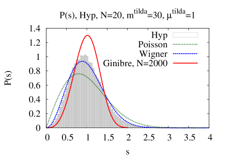
Figure 4: The NNS distribution of the Hyp notation at $N=20$, $\tilde{m}=2$, and $\tilde{\mu}=1$.

Figure 5: The NNS distribution of the Hyp notation at $N=20$, $\tilde{m}=30$, and $\tilde{\mu}=1$.

We show the NNS distribution in the Hyp representation for ($\tilde{\mu},\tilde{m})=(1,2)$ and (1,30) in Figs. 5 and 5, respectively. The NNS distributions at $\tilde{m}=2$ and $30$ are almost consistent with the Wigner surmise.

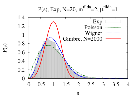
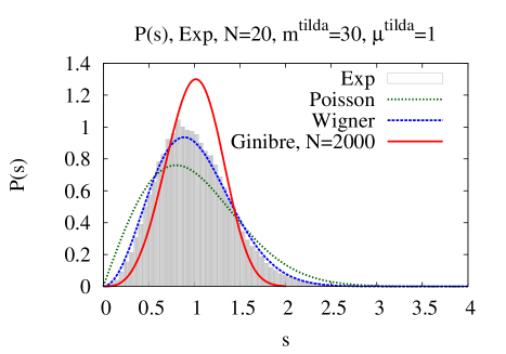
Figure 6: The NNS distribution of the Exp notation at $N=20$, $\tilde{m}=2$, and $\tilde{\mu}=1$.

Figure 7: The NNS distribution of the Exp notation at $N=20$, $\tilde{m}=30$, and $\tilde{\mu}=1$.

We show the NNS distribution in the Exp representation for ($\tilde{\mu},\tilde{m})=(1,2)$ and (1,30) in Figs. 7 and 7, respectively. For $\tilde{m}=30$, the NNS distribution in the Exp representation is almost the same as that in the Hyp representation. By comparison, the NNS distribution at $\tilde{m}=2$ is slightly different from NNS distribution at $\tilde{m}=30$ and is relatively close to the Wigner surmise.

For small $\tilde{m}$, the NNS distributions in the two representations are slightly different. The difference increases for $\tilde{\mu}=3$ as we will show in the next subsection.

IV.2 Results for $N=20$ at $\tilde{\mu}=3$

In Fig. 8, we show the chiral condensate at $\tilde{\mu}=3$ as a function of $\tilde{m}$. The chiral condensate in the Exp representation reproduces the correct result shown by the solid line, as found in Mollgaard and Splittorff (2015). On the other hand, the chiral condensate in the Hyp representation produces results close to the phase quenched theory shown by dotted line at low $\tilde{m}$.

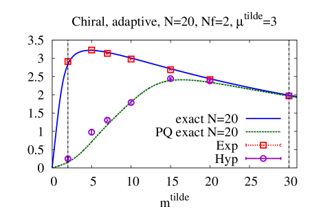
Figure 8: Chiral condensate at $\tilde{\mu}=3$ as a function of $\tilde{m}$. The solid line shows the exact value in the ChRMT Osborn (2004) and the dotted line shows the exact value in the phase quenched (PQ) ChRMT Akemann et al. (2005). The results of the Exp and Hyp representations are expressed as squares and circles. At large $\tilde{m}$, both the representations well produce the exact result. The result of Hyp representation at small $\tilde{m}$ deviates from the exact result. Dotted vertical lines show the values of $\tilde{m}$ at which the NNS distribution is obtained.

We show the NNS distributions in the Hyp representation for ($\tilde{\mu},\tilde{m})=(3,2)$ and (3,30) in Figs. 10 and 10, respectively. The NNS distributions in those cases are approximately consistent with each other, but slightly smaller than the Ginibre ensemble. We do not find strong $\tilde{m}$ dependence of the NNS distribution in the Hyp representation.

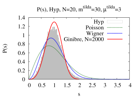
Figure 9: The NNS distribution of the Hyp notation at $N=20$, $\tilde{m}=2$, and $\tilde{\mu}=3$.

Figure 10: The NNS distribution of the Hyp notation at $N=20$, $\tilde{m}=30$, and $\tilde{\mu}=3$.

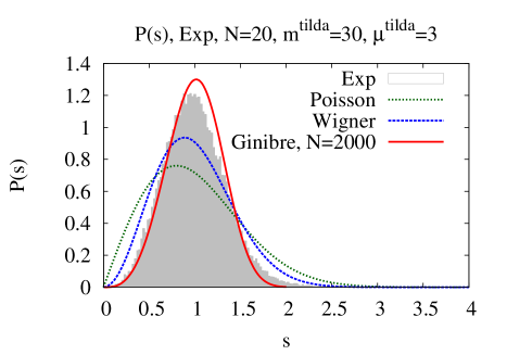
Figure 11: The NNS distribution of the Exp notation at $N=20$, $\tilde{m}=2$, and $\tilde{\mu}=3$.

Figure 12: The NNS distribution of the Exp notation at $N=20$, $\tilde{m}=30$, and $\tilde{\mu}=3$.

Next, we show the NNS distribution in the Exp representation for ($\tilde{\mu},\tilde{m})=(3,2)$ and (3,30) in Figs. 12 and 12, respectively. We find that the NNS distributions depend on $\tilde{m}$. At small $\tilde{m}$, the NNS distribution is close to the Wigner surmise. At large $\tilde{m}$, the NNS distribution approximately follows that in the Ginibre ensemble, and is almost consistent with that in the Hyp representation.

IV.3 Discussion

Now, we discuss the interpretation of our results and its implications. We found that the Ginibre ensemble is favored at large $\tilde{m}$ in both representations. This is physically reasonable, because the fermion determinant is approximated by the mass factor as $\det({\ooalign{\hfil/\hfil\crcr$D$}}+m)\sim m^{2N}$. There is no difference between the original theory and phase quenched theory, and both of them provide the same results. In this case, the partition function is well described as the Gaussian form of the complex matrices $\Phi_{1,2}$, which is nothing but the Ginibre ensemble Ginibre (1965); Verbaarschot (2005).

On the other hand, we found that at small $\tilde{m}$ the Wigner surmise and Ginibre ensemble are favored in the Exp and Hyp representation, respectively. The ChRMT used in this work is independent of quark chemical potential $\mu$  Osborn (2004); Bloch et al. (2013), which implies that the NNS distribution at finite $\mu$ should be the same with that at zero $\mu$. As we have explained, the Wigner surmise is theoretically expected at $\mu=0$. Thus, we find that the NNS distribution shows physically expected behavior even in the CL method, if the Langevin simulation converges to the correct results. The Ginibre ensemble in the Hyp representation is caused by unphysical broadening of the Dirac eigenvalue distribution due to the failure of the complex Langevin simulation.

Here, we should note that there is a subtlety in the application of the CL method to the NNS distribution. The argument to justify the CL method is given for holomorphic observables Aarts et al. (2010a, 2011), while it is unclear if the CL method can be justified for non-holomorphic observables. The NNS distribution is real, and therefore a non-holomorphic quantity. It is not ensured that the NNS distribution obtained in the CL method agrees with that in the original theory. Although the Dirac eigenvalue distribution is narrower for the correct convergence case, the distribution more or less receives broadening caused by the complexification, namely imaginary parts of the originally real variables. In this sense, it is non-trivial that the CL method can reproduce the physical behavior of the NNS distribution.

As we mentioned in the Introduction, we conjecture that the NNS distribution, a universal quantity defined for the Dirac eigenvalues, can provide physical behavior even in the complex Langevin simulation. Although this is highly non-trivial statement due to the non-holomorphy of the NNS distribution, our numerical results support this conjecture. Such a conjecture may be also inferred from an analogy between the CL method and the Lefshetz thimble (LT) method. In the LT method, dominant critical points are expected to share the symmetry properties with an original integral contour as shown in the case of one classical thimble contribution Cristoforetti et al. (2012). In the CL and LT methods, the critical points are located at the same points on the complex plane, and therefore dominant critical points in the CL method are also expected to share the symmetry properties of the original theory. If this conjecture holds, the universal quantities may provide a tool to understand the convergence properties of the CL simulations, which will be useful in the study of theories where exact results are not known such as in QCD.

V Summary

In this work, we have performed the first study of the nearest neighbor spacing (NNS) distributions of Dirac eigenvalues in the chiral random matrix theory (ChRMT) at non zero quark chemical potential using the complex Langevin (CL) method. The ChRMT was described in two representations: the hyperbolic and exponential forms of the chemical potential. The polar coordinate was adopted in both cases for the description of dynamical variables. For small quark mass, the hyperbolic case converges to the wrong result and exponential case converges to the correct result, as shown in a previous study Mollgaard and Splittorff (2015).

We have calculated the NNS distribution for several values of the mass and chemical potential using the unfolding procedure. For large mass, the NNS distribution follows the Ginibre ensemble, which implies that the real and imaginary part of the Dirac eigenvalues have the same order of magnitude. For small mass, we found the deviation between two representations. The NNS distribution follows the Wigner surmise for the correctly converging case, while it follows the Ginibre ensemble when the simulation converges to the phase quenched result. The Wigner surmise is physically reasonable according to the chemical potential independence of the ChRMT. Thus, the NNS distribution shows the physical behavior even in the CL method if it converges to the correct result.

There is a subtlety as to whether the NNS distribution, which is non-holomorphic, can be justified in the CL method. We speculate from the analogy between the CL and Lefshetz thimble methods that universal quantities determined from the properties such as symmetries can be maintained even in the CL method if the configurations are correctly located around relevant critical points. If this holds, the universal quantities can be used to test the convergence properties of the CL method. At least, our numerical result support this conjecture. Of course, it is important to consider the theoretical justification of the conjecture and applications to other universal quantities and to other theories, which we leave for future studies. Such a study will deepen our understanding of complexified theories, and may provide information about a convergence property in the CL simulation for the study of theories with the sign problem.

Appendix A Drift terms

The drift terms for the angular and radius variables in the CL equations with the Hyp notation are gives as

$$-\frac{\partial S}{\partial\theta_{1,mn}} =-N_{f}\left[G_{ij}\partial_{\theta_{1,mn}}(X_{jk}Y_{ki})\right]$$

$$=-N_{f}\cosh(\mu)\left[G_{ij}(X_{jk}r_{1,ik}e^{-i\theta_{1,ik}}\delta_{mi}\delta_{nk}-\delta_{mj}\delta_{nk}r_{1,jk}e^{i\theta_{1,jk}}Y_{ki})\right]$$

$$=-N_{f}\cosh(\mu)\left[G_{mj}X_{jn}r_{1,mn}e^{-i\theta_{1,mn}}-G_{im}r_{1,mn}e^{i\theta_{1,mn}}Y_{ni}\right]$$

$$=-N_{f}\cosh(\mu)\left[(GX)_{mn}r_{1,mn}e^{-i\theta_{1,mn}}-(YG)_{nm}r_{1,mn}e^{i\theta_{1,mn}}\right]$$

$$=-N_{f}\cosh(\mu)r_{1,mn}\left[(GX)_{mn}e^{-i\theta_{1,mn}}-\left((YG)^{t}\right)_{mn}e^{i\theta_{1,mn}}\right]\ ,$$ (29)

$$-\frac{\partial S}{\partial\theta_{2,mn}} =-N_{f}\left[G_{ij}\partial_{\theta_{2,mn}}(X_{jk}Y_{ki})\right]$$

$$=-iN_{f}\sinh(\mu)\left[G_{ij}(X_{jk}r_{2,ki}e^{i\theta_{2,ki}}\delta_{km}\delta_{in}-\delta_{km}\delta_{jn}r_{2,kj}e^{-i\theta_{2,kj}}Y_{ki})\right]$$

$$=-iN_{f}\sinh(\mu)\left[G_{nj}X_{jm}r_{2,mn}e^{i\theta_{2,mn}}-G_{in}r_{2,mn}e^{-i\theta_{2,mn}}Y_{mi}\right]$$

$$=-iN_{f}\sinh(\mu)r_{2,mn}\left[\left((GX)^{t}\right)_{mn}e^{i\theta_{2,mn}}-\left(YG\right)_{mn}e^{-i\theta_{2,mn}}\right]\ ,$$ (30)

$$-\frac{\partial S}{\partial r_{1,mn}} =-2Nr_{1,mn}+\frac{1}{r_{1,mn}}-N_{f}[G_{ij}\partial_{r_{1,mn}}X_{jk}Y_{ki}]$$

$$=-2Nr_{1,mn}+\frac{1}{r_{1,mn}}-iN_{f}\cosh(\mu)[G_{ij}\left(e^{i\theta_{1,jk}}\delta_{jm}\delta_{kn}Y_{ki}+X_{jk}e^{-i\theta_{1,ik}}\delta_{mi}\delta_{nk}\right)]$$

$$=-2Nr_{1,mn}+\frac{1}{r_{1,mn}}-iN_{f}\cosh(\mu)[G_{im}e^{i\theta_{1,mn}}Y_{ni}+G_{mj}X_{jn}e^{-i\theta_{1,mn}}]$$

$$=-2Nr_{1,mn}+\frac{1}{r_{1,mn}}-iN_{f}\cosh(\mu)[\left((YG)^{t}\right)_{mn}e^{i\theta_{1,mn}}+\left(GX\right)_{mn}e^{-i\theta_{1,mn}}]\ ,$$ (31)

$$-\frac{\partial S}{\partial r_{2,mn}} =-2Nr_{2,mn}+\frac{1}{r_{2,mn}}-N_{f}[G_{ij}\partial_{r_{2,mn}}X_{jk}Y_{ki}]$$

$$=-2Nr_{2,mn}+\frac{1}{r_{2,mn}}-N_{f}\sinh(\mu)[G_{ij}\left(e^{-i\theta_{2,kj}}\delta_{km}\delta_{jn}Y_{ki}+X_{jk}e^{i\theta_{2,ki}}\delta_{mk}\delta_{ni}\right)]$$

$$=-2Nr_{2,mn}+\frac{1}{r_{2,mn}}-N_{f}\sinh(\mu)[G_{in}e^{-i\theta_{2,mn}}Y_{mi}+G_{nj}X_{jm}e^{i\theta_{2,mn}}]$$

$$=-2Nr_{2,mn}+\frac{1}{r_{2,mn}}-N_{f}\sinh(\mu)[\left(YG\right)_{mn}e^{-i\theta_{2,mn}}+\left((GX)^{t}\right)_{mn}e^{i\theta_{2,mn}}]\ ,$$ (32)

where we use a formula, $(\det X)^{{}^{\prime}}=\det X\ \mathrm{Tr}(X^{-1}X^{{}^{\prime}})$.

Appendix B Results on the nearest neighbor distributions with two fitting function

In Figs. 13 and 14, the NNS distributions in Hyp and Exp with two fitting functions. The dependence of the fitting functions seems to be small for the NNS distributions. Then, we adopt a quintic function to obtain the NNS distributions in this paper.

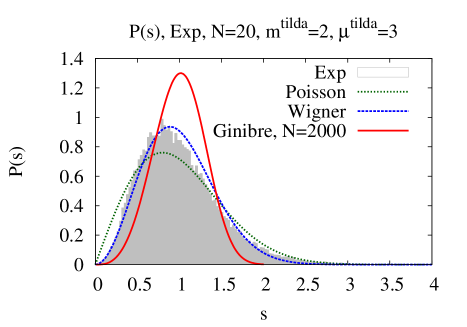
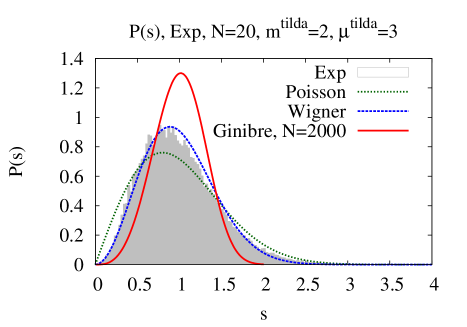
Figure 13: The NNS distribution at $N=20$, $\tilde{m}=2$, and $\tilde{\mu}=3$ in Exp with a cubic fitting function in the top panel and that with a quintic fitting function in the bottom panel.

Figure 14: The NNS distribution at $N=20$, $\tilde{m}=2$, and $\tilde{\mu}=3$ in Hyp with a cubic fitting function in the top panel and that with a quintic fitting function in the bottom panel.

References

- Parisi (1983) G. Parisi, Phys. Lett. B 131, 393 (1983).
- Klauder (1984) J. R. Klauder, Phys. Rev. A 29, 2036 (1984).
- Seiler et al. (2013) E. Seiler, D. Sexty, and I.-O. Stamatescu, Phys. Lett. B 723, 213 (2013), eprint 1211.3709.
- Pham (1983) F. Pham, Proc. Symp. Pure Math. 40, 319 (1983).
- Witten (2011) E. Witten, AMS/IP Stud. Adv. Math. 50, 347 (2011), eprint 1001.2933.
- Witten (2010) E. Witten (2010), eprint 1009.6032.
- Parisi and Wu (1981) G. Parisi and Y.-S. Wu, Sci. Sin. 24, 483 (1981).
- Namiki et al. (1992) M. Namiki, I. Ohba, K. Okano, Y. Yamanaka, A. K. Kapoor, H. Nakazato, and S. Tanaka, Lect. Notes Phys. M9, 1 (1992).
- Damgaard and Huffel (1987) P. H. Damgaard and H. Huffel, Phys. Rept. 152, 227 (1987).
- Aarts et al. (2010a) G. Aarts, E. Seiler, and I.-O. Stamatescu, Phys. Rev. D 81, 054508 (2010a), eprint 0912.3360.
- Aarts et al. (2011) G. Aarts, F. A. James, E. Seiler, and I.-O. Stamatescu, Eur. Phys. J. C 71, 1756 (2011), eprint 1101.3270.
- Mollgaard and Splittorff (2013) A. Mollgaard and K. Splittorff, Phys. Rev. D 88, 116007 (2013), eprint 1309.4335.
- Greensite (2014) J. Greensite, Phys. Rev. D 90, 114507 (2014), eprint 1406.4558.
- Nishimura and Shimasaki (2015) J. Nishimura and S. Shimasaki, Phys. Rev. D 92, 011501 (2015), eprint 1504.08359.
- Sexty (2014) D. Sexty, Phys. Lett. B 729, 108 (2014), eprint 1307.7748.
- Fodor et al. (2015) Z. Fodor, S. D. Katz, D. Sexty, and C. Török, Phys. Rev. D 92, 094516 (2015), eprint 1508.05260.
- Nagata et al. (2016) K. Nagata, J. Nishimura, and S. Shimasaki, Progress of Theoretical and Experimental Physics 2016, 013B01 (2016), eprint 1508.02377.
- Nagata et al. (2015) K. Nagata, J. Nishimura, and S. Shimasaki, in Proceedings, 33rd International Symposium on Lattice Field Theory (Lattice 2015) (2015), eprint 1511.08580, URL https://inspirehep.net/record/1406950/files/arXiv:1511.08580.pdf.
- Mollgaard and Splittorff (2015) A. Mollgaard and K. Splittorff, Phys. Rev. D 91, 036007 (2015), eprint 1412.2729.
- Cristoforetti et al. (2012) M. Cristoforetti, F. Di Renzo, and L. Scorzato (AuroraScience Collaboration), Phys. Rev. D 86, 074506 (2012), eprint 1205.3996.
- Markum et al. (1999) H. Markum, R. Pullirsch, and T. Wettig, Phys. Rev. Lett. 83, 484 (1999), eprint hep-lat/9906020.
- Stephanov (1996) M. A. Stephanov, Phys. Rev. Lett. 76, 4472 (1996), eprint hep-lat/9604003.
- Osborn (2004) J. C. Osborn, Phys. Rev. Lett. 93, 222001 (2004), eprint hep-th/0403131.
- Bloch et al. (2013) J. Bloch, F. Bruckmann, M. Kieburg, K. Splittorff, and J. J. M. Verbaarschot, Phys. Rev. D 87, 034510 (2013), eprint 1211.3990.
- Ambjorn et al. (1986) J. Ambjorn, M. Flensburg, and C. Peterson, Nucl. Phys. B 275, 375 (1986).
- Aarts et al. (2010b) G. Aarts, F. A. James, E. Seiler, and I.-O. Stamatescu, Phys. Lett. B 687, 154 (2010b), eprint 0912.0617.
- Aarts and James (2010) G. Aarts and F. A. James, JHEP 08, 020 (2010), eprint 1005.3468.
- Akemann et al. (2005) G. Akemann, J. C. Osborn, K. Splittorff, and J. J. M. Verbaarschot, Nucl. Phys. B 712, 287 (2005), eprint hep-th/0411030.
- Guhr et al. (1998) T. Guhr, A. Muller-Groeling, and H. A. Weidenmuller, Phys. Rept. 299, 189 (1998), eprint cond-mat/9707301.
- Verbaarschot and Wettig (2000) J. J. M. Verbaarschot and T. Wettig, Annu. Rev. Nucl. Part. Sci. 50, 343 (2000), eprint hep-ph/0003017.
- Halasz and Verbaarschot (1995) M. A. Halasz and J. J. M. Verbaarschot, Phys. Rev. Lett. 74, 3920 (1995), eprint hep-lat/9501025.
- Ginibre (1965) J. Ginibre, J. Math. Phys. 6, 440 (1965).
- Grobe et al. (1988) R. Grobe, F. Haake, and H.-J. Sommers, Phys. Rev. Lett. 61, 1899 (1988).
- Verbaarschot (2005) J. J. M. Verbaarschot, in Application of random matrices in physics. Proceedings, NATO Advanced Study Institute, Les Houches, France, June 6-25, 2004 (2005), pp. 163–217, eprint hep-th/0502029.