Scalar multi-wormholes

Abstract

In 1921 Bach and Weyl derived the method of superposition to construct new axially symmetric vacuum solutions of General Relativity. In this paper we extend the Bach-Weyl approach to non-vacuum configurations with massless scalar fields. Considering a phantom scalar field with the negative kinetic energy, we construct a multi-wormhole solution describing an axially symmetric superposition of $N$ wormholes. The solution found is static, everywhere regular and has no event horizons. These features drastically tell the multi-wormhole configuration from other axially symmetric vacuum solutions which inevitably contain gravitationally inert singular structures, such as ‘struts’ and ‘membranes’, that keep the two bodies apart making a stable configuration. However, the multi-wormholes are static without any singular struts. Instead, the stationarity of the multi-wormhole configuration is provided by the phantom scalar field with the negative kinetic energy. Anther unusual property is that the multi-wormhole spacetime has a complicated topological structure. Namely, in the spacetime there exist $2^{N}$ asymptotically flat regions connected by throats.

I Introduction

The two-body (and, more generally, $N$-body) problem is one of the most important and interesting to be solved in any theory of gravity. It is well known that in Newtonian gravity this problem is well-defined and, in the two-body case $N=2$, has a simple exact treatment of the solution. In general relativity the $N$-body problem has been investigated from the early days of Einstein’s gravitation theory Dro ; DeSitter ; LorDro ; LC ; EinInfHof . However, because of conceptual and technical difficulties the motion of the $N$ bodies cannot be solved exactly in the context of general relativity, even when $N=2$. Hence analysis of a two body system (e.g. binary pulsars) necessarily involves resorting to approximation methods such as a post-Newtonian expansion (see, e.g., Damour ; Blanchet for a review and references to the early literature).

Besides developing approximate methods for solving the $N$-body problem, essential efforts had been undertaken to search and study exact solutions of the Einstein equations which could be interpreted as that describing multi-particle configurations in general relativity. At the early days of general relativity Weyl Weyl and Levi-Civita LeviCivita demonstrated that static axially symmetric gravitational fields can be described by the following metric (now known as the Weyl metric):

$$ds^{2}=-e^{2\lambda}dt^{2}+e^{-2\lambda}\left[e^{2\nu}(d\rho^{2}+dz^{2})+\rho^{2}d\varphi^{2}\right],$$ (1)

where the functions $\lambda$ and $\nu$ depend on coordinates $\rho$ and $z$ only. In vacuum, when $R_{\mu\nu}=0$, these functions satisfy, respectively, the Laplace equation

$$\Delta\lambda=\lambda_{,\rho\rho}+\lambda_{,zz}+\frac{\lambda_{,\rho}}{\rho}=0,$$ (2)

and two partial differential equations

$$\nu_{,\rho}=\rho(\lambda_{,\rho}^{2}-\lambda_{,z}^{2}),$$ (3)

$$\nu_{,z}=2\rho\lambda_{,\rho}\lambda_{,z},$$ (4)

where a comma denotes a partial derivative, e.g. $\lambda_{,\rho}={\partial\lambda}/{\partial\rho}$, $\lambda_{,\rho\rho}={\partial^{2}\lambda}/{\partial\rho^{2}}$, etc. Since 2 is linear and homogeneous, the superposition of any integrals is again an integral of that equation. This fact and the particular form of Eqs. 3, 4 allows us to find explicitly solutions that represent the superposition of two or more axially symmetric bodies of equal or different shapes. In the pioneering work BachWeyl , Bach and Weyl obtained an axially symmetric vacuum solution interpreted as equilibrium configurations of a pair of Schwarzschild black holes. Since then, the fruitful Bach-Weyl method has been used to construct a number of exact axially symmetric vacuum solutions Chazy ; Curzon ; Chou ; Synge ; Bondi ; IsraelKhan ; Letelier:87 ; Letelier:88 . It is worth noticing that all solutions, representing the superposition of two or more axially symmetric bodies, contain gravitationally inert singular structures, ‘struts’ and ‘membranes’, that keep the two bodies apart making a stable configuration. This is an expected “price to pay” for the stationarity BachWeyl ; EinsteinRosen ; Cooperstock ; Tomimatsu ; Yamazaki ; Schleifer .

The advances of the Bach-Weyl approach in constructing exact axially symmetric solutions are based on the specific algebraic form of the vacuum field equations 2-4. However, in this paper we demonstrate that this approach can be easily extended to gravitating systems with a massless scalar field $\phi$. Though such the systems are not vacuum ones, we show that new axially symmetric solutions with the scalar field can be found as a superposition of known spherically symmetric configurations. More specifically, we construct and analyze a multi-wormhole configuration with the phantom scalar field that possesses the negative kinetic energy.

The paper is organized as follows. In the section II we consider the theory of gravity with a massless scalar field and derive field equations for a static axially symmetric configuration. In the section III we review solutions describing spherically symmetric scalar wormholes. In the section IV we construct multi-wormhole solutions. First, we consider specific properties of a single-wormhole axially symmetric configuration. Then, using the superposition method, we discuss in detail the procedure of constructing of two-wormhole solution, and, more generally, $N$-wormhole one. In the concluding section we summarize results and give some remarks concerning the regularity of the solutions and the violation of the null energy condition.

II Field equations

The theory of gravity with a massless scalar field $\phi$ is described by the action

$$S=\int d^{4}x\sqrt{-g}\left[R-\epsilon g^{\mu\nu}\phi_{,\mu}\phi_{,\nu}\right],$$ (5)

where $g_{\mu\nu}$ is a metric, $g=\det(g_{\mu\nu})$, and $R$ is the scalar curvature. The parameter $\epsilon$ equals $\pm 1$. In the case $\epsilon=1$ we have a canonical scalar field with the positive kinetic term, and the case $\epsilon=-1$ describes a phantom scalar field with the negative kinetic energy. It is well-known that wormholes in the theory 5 exist only if the scalar field is phantom, and so hereinafter we will assume that $\epsilon=-1$.

Varying the action 5 with respect to $g_{\mu\nu}$ and $\phi$ leads to the field equations

$$R_{\mu\nu}=-\phi_{,\mu}\phi_{,\nu},$$ (6a)

$$\square\phi=0.$$ (6b)

Let us search for static axially symmetric solutions of Eqs. 6. In this case a gravitational field is described by the canonical Weyl metric 1, and the scalar field $\phi$ depends on coordinates $\rho$ and $z$ only. Now the field equations 6 can be represented in the following form

$$\Delta\lambda=0,$$ (7a)

$$\Delta\phi=0,$$ (7b)

$$\nu_{,\rho}=\rho\left[\lambda_{,\rho}^{2}-\lambda_{,z}^{2}-\textstyle\frac{1}{2}(\phi_{,\rho}^{2}-\phi_{,z}^{2})\right],$$ (7c)

$$\nu_{,z}=\rho\left[2\lambda_{,\rho}\lambda_{,z}-\phi_{,\rho}\phi_{,z}\right].$$ (7d)

Here it is necessary to emphasize that the functions $\lambda(\rho,z)$ and $\phi(\rho,z)$ satisfy the Laplace equations 7a, 7b, where $\textstyle\Delta=\frac{1}{\rho}\frac{\partial}{\partial\rho}\left(\rho\frac{\partial}{\partial\rho}\right)+\frac{\partial^{2}}{\partial z^{2}}$ is the Laplace operator in cylindrical coordinates. Since 7a, 7b are linear and homogeneous, superpositions of any integrals are again integrals of that equations. Then, since $\nu_{,\rho z}=\nu_{,z\rho}$, Eqs. 7c, 7d yield

$$2\lambda_{,z}\Delta\lambda+\phi_{,z}\Delta\phi=0.$$

The latter is fulfilled due to 7a and 7b, and so Eqs. 7a, 7b are integrability conditions for Eqs. 7c, 7d. Therefore, provided solutions $\lambda(\rho,z)$ and $\phi(\rho,z)$ of Eqs. 7a, 7b are given, Eqs. 7c, 7d can be integrated in terms of the line integral

$$\nu(\rho,z)=\int_{\cal C}\rho\big{[}\lambda_{,\rho}^{2}-\lambda_{,z}^{2}-{\textstyle\frac{1}{2}}(\phi_{,\rho}^{2}-\phi_{,z}^{2})\big{]}d\rho+\rho\big{[}2\lambda_{,\rho}\lambda_{,z}-\phi_{,\rho}\phi_{,z}\big{]}dz,$$ (8)

where $\cal C$ is an arbitrary path connecting some fixed point $(\rho_{0},z_{0})$ with the point $(\rho,z)$. In practice, a choice of $(\rho_{0},z_{0})$ is determined by the boundary condition $\nu(\rho_{0},z_{0})=\nu_{0}$.

III Spherically symmetric wormhole solution

Wormholes are usually defined as topological handles in spacetime linking widely separated regions of a single universe, or “bridges” joining two different spacetimes MorTho ; VisserBook . As is well-known HocVis1 ; HocVis2 , in the framework of general relativity they can exist only if their throats contain an exotic matter which possesses a negative pressure and violates the null energy condition. The simplest model which provides the necessary conditions for existence of wormholes is the theory of gravity 5 with the phantom scalar field. Static spherically symmetric wormholes in the model 5 were obtained by Ellis Ellis and Bronnikov Bro_73 . Adapting their result (see Ref. SusKim ), one can write down a wormhole solution as follows

$$ds^{2}=-e^{2\lambda(r)}dt^{2}+e^{-2\lambda(r)}\left[dr^{2}+(r^{2}+a^{2})\left(d\theta^{2}+\sin^{2}\theta d\varphi^{2}\right)\right],$$ (9)

$$\phi(r)=\frac{\sqrt{2(m^{2}+a^{2})}}{m}\,\lambda(r),$$ (10)

where

$$\lambda(r)=\frac{m}{a}\arctan({r}/{a}),$$ (11)

$r\in(-\infty,\infty)$, and $m$ and $a$ are two free parameters. In the case $m=0$ one has $\lambda(r)=0$, and the solution 9, 10 takes the especially simple form:

$$ds^{2}=-dt^{2}+dr^{2}+(r^{2}+a^{2})\left(d\theta^{2}+\sin^{2}\theta d\varphi^{2}\right),$$ (12)

$$\phi(r)=\sqrt{2}\,\arctan({r}/{a}).$$ (13)

The latter describes a massless wormhole connecting two asymptotically flat regions at $r\to\pm\infty$. The throat of the wormhole is located at $r=0$ and has the radius $a$. The scalar field $\phi$ smoothly varies between two asymptotical values $\pm\pi/\sqrt{2}$.

Hereafter, for simplicity, we will assume that $m=0$ and hence $\lambda=0$.

IV Multi-wormhole solution

IV.1 Single wormhole

Let us consider an axially symmetric form of the spherically symmetric wormhole solution given in the previous section. For this aim we rewrite the solution 12-13 in cylindrical coordinates $(\rho,z)$ carrying out the coordinate transformation

$$\rho = \sqrt{r^{2}+a^{2}}\sin\theta,$$ (14a)

$$z = r\cos\theta.$$ (14b)

The corresponding Jacobian reads

$$J=\frac{D(\rho,z)}{D(r,\theta)}=-\frac{r^{2}+a^{2}\cos^{2}\theta}{\sqrt{r^{2}+a^{2}}}.$$ (15)

Since the Jacobian $J$ is equal to zero at $r=0,\theta=\frac{\pi}{2}$, the transformation 14 is degenerated at this point.

Remind ourselves that in the wormhole spacetime the proper radial coordinate $r$ runs from $-\infty$ to $+\infty$, while the azimuthal coordinate $\theta$ runs from $0$ to $\pi$. Therefore, the domain of spherical coordinates $(r,\theta)$ can be represented as the strip ${\cal S}=(-\infty,\infty)\times[0,\pi]$ on the plane $\mathbb{R}\times\mathbb{R}$ (see Fig. 1). Note that the wormhole throat is represented as the segment ${\cal T}=\{r=0,\theta\in[0,\pi]\}$ on ${\cal S}$. The regions with $r\to\pm\infty$ on the strip $\cal S$ correspond to two asymptotically flat regions of the wormhole spacetime. The corresponding domain of cylindrical coordinates $(\rho,z)$ is found from 14 as the half-plane ${\cal D}=[0,\infty)\times(-\infty,\infty)$. Correspondingly, the wormhole throat is represented as the segment ${\cal T}_{a}=\{\rho\in[0,a],z=0\}$ on ${\cal D}$, where $a$ is the radius of the throat. Note also that the asymptotics $r\to\pm\infty$ in cylindrical coordinates take the form $(\rho^{2}+z^{2})^{1/2}\to\infty$.

The transformation 14 determines the mapping ${\cal S}\to{\cal D}$. It is necessary to emphasize that it maps two different points of $\cal S$ into a single point of $\cal D$. Namely, $(r,\theta)\to(\rho,z)$ and $(-r,\pi-\theta)\to(\rho,z)$. Therefore, the mapping ${\cal S}\to{\cal D}$ is not bijective. To construct a bijective mapping, we first consider two half-strips, ${\cal S}_{-}=(-\infty,0)\times[0,\pi]$ and ${\cal S}_{+}=(0,\infty)\times[0,\pi]$, which represent, respectively, ‘lower’ ($r<0$) and ‘upper’ ($r>0$) halves of the wormhole spacetime. The edge of both half-stripes is the segment $\cal T$, which, in turn, corresponds to the wormhole’s throat. Additionally, we introduce two identical copies of the half-plane ${\cal D}$ denoted as ${\cal D}_{\pm}$; the segments ${\cal T}_{a\pm}$ on ${\cal D}_{\pm}$ correspond to the wormhole’s throat. Now, each of the mapping ${\cal S}_{\pm}\to{\cal D}_{\pm}$ is bijective. The whole strip $\cal S$ is restored by means of the gluing of two half-strips ${\cal S}_{\pm}$ along their common edge $\cal T$. This procedure corresponds to the topological gluing of two half-planes ${\cal D}_{\pm}$ by means of identifying corresponding points of the segments ${\cal T}_{a\pm}$. As the result of this topological gluing, one obtains a new manifold denoted as $\overline{\cal D}{}_{2}$, consisting of two sheets ${\cal D}_{\pm}$ with the common segment ${\cal T}_{a}$. It is worth noticing that the manifold $\overline{\cal D}{}_{2}$ is homeomorphic to the self-crossing two-sheeted Riemann surface. The sheets ${\cal D}_{\pm}$ of the manifold $\overline{\cal D}{}_{2}$ contain asymptotically flat regions $(\rho^{2}+z^{2})^{1/2}\to\infty$ connecting by the throat $\cal T$. Now, the mapping ${\cal S}\to\overline{\cal D}{}_{2}$ is a bijection. Schematically, the mapping ${\cal S}_{\pm}\to{\cal D}_{\pm}$ is shown in Fig. 1. Respectively, in Fig. 2 we illustrate the procedure of constructing the manifold $\overline{\cal D}{}_{2}$ by means of topological gluing.

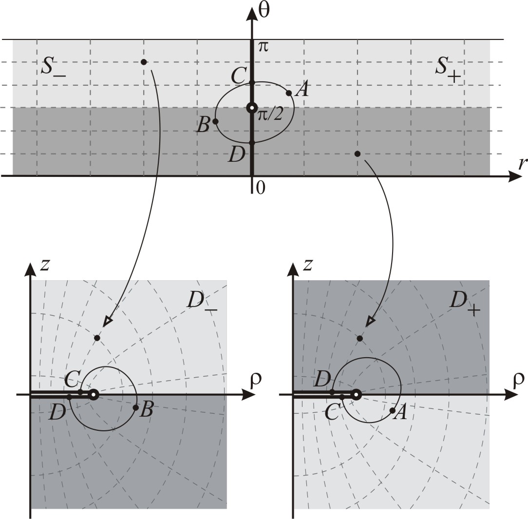
Figure 1: The mapping ${\cal S}\to\overline{\cal D}{}_{2}$ is shown. The regions ${\cal S}_{+}$ and ${\cal S}_{-}$ are mapped to ${\cal D}_{+}$ and ${\cal D}_{-}$ correspondingly. The segment ${\cal T}=\{r=0,\theta\in[0,\pi]\}$ in ${\cal S}$ corresponds to the wormhole’s throat and it is mapped to two-sided segment ${\cal T}_{a\pm}=\{\rho\in[0,a],z=0\}$ in ${\cal D}_{\pm}$. Note that the upper part $\{r=0,\theta\in[\pi/2,\pi]\}$ of the throat ${\cal T}$ correspons to the upper part of the two-sided segment ${\cal T}_{a-}$ in ${\cal D}_{-}$ and the lower part of the ${\cal T}_{a+}$ in ${\cal D}_{+}$, while the lower part $\{r=0,\theta\in[0,\pi/2]\}$ of the throat ${\cal T}$ corresponds to the lower part of the two-sided segment ${\cal T}_{a-}$ of ${\cal D}_{-}$ and the upper part of the segment ${\cal T}_{a+}$ of ${\cal D}_{+}$.

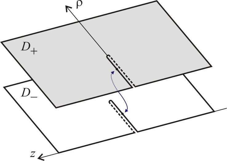
Figure 2: The manifold $\overline{\cal D}_{2}$ consists of two regions ${\cal D}_{\pm}$, which are glued together by the two-sided segments ${\cal T}_{a\pm}$.

The transformation being inverse to 14 reads

$$r = \pm R(\rho,z),$$ (16a)

$$\theta = \arccos\big{(}{z}/{R(\rho,z)}\big{)},$$ (16b)

where

$$R(\rho,z)=\frac{1}{\sqrt{2}}\left[(\rho^{2}+z^{2}-a^{2})+\sqrt{(\rho^{2}+z^{2}-a^{2})^{2}+4a^{2}z^{2}}\right]^{1/2}.$$ (17)

Performing the transformation 16, we obtain the single-wormhole metric 12 in Weyl coordinates:

$$ds_{\pm}^{2}=-dt^{2}+e^{2\nu_{\pm}}[d\rho^{2}+dz^{2}]+\rho^{2}d\varphi^{2},$$ (18)

where

$$\nu_{\pm}(\rho,z)=\frac{1}{2}\ln\left[\frac{R^{2}(\rho,z)\big{(}R^{2}(\rho,z)+a^{2}\big{)}}{R^{4}(\rho,z)+a^{2}z^{2}}\right],$$ (19)

and the scalar field 13 now reads

$$\phi_{\pm}(\rho,z)=\pm\sqrt{2}\arctan\big{(}{R(\rho,z)}/{a}\big{)}.$$ (20)

The signs $\pm$ in Eqs. 16-20 are pointing out that the metric $ds^{2}_{\pm}$, as well as the functions $\phi_{\pm}(\rho,z)$ and $\nu_{\pm}(\rho,z)$ are defined on the respective charts ${\cal D}_{\pm}$, i.e. one should choose the plus sign if $(\rho,z)\in{\cal D}_{+}$ ($r>0$), and minus if $(\rho,z)\in{\cal D}_{-}$ ($r<0$). The complete solutions defined on the whole manifold $\overline{\cal D}{}_{2}$ are constituted from separate $\phi_{\pm}(\rho,z)$ and $\nu_{\pm}(\rho,z)$. In particular, the scalar field $\phi(\rho,z)$ on $\overline{\cal D}{}_{2}$ is defined as follows:

$$\phi(\rho,z)=\left\{\begin{array}[]{ll}\phi_{-}(\rho,z)&\mathrm{if}\ (\rho,z)\in{\cal D}_{-}\\ \phi_{+}(\rho,z)&\mathrm{if}\ (\rho,z)\in{\cal D}_{+}\end{array}\right.$$ (21)

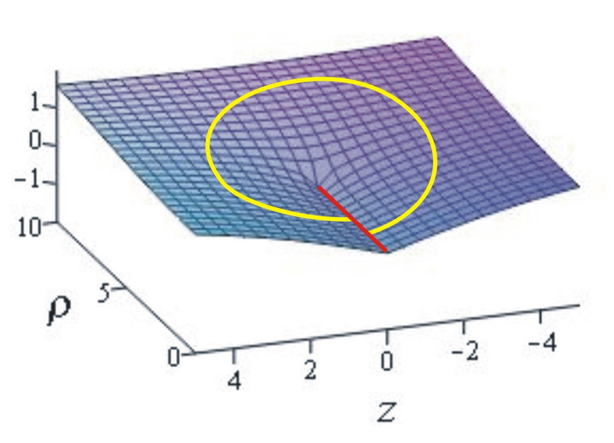
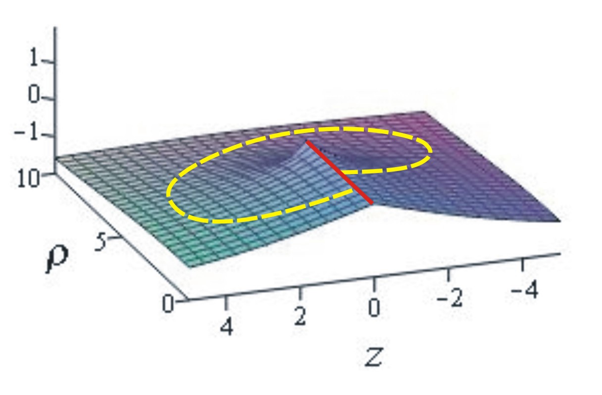
Figure 3: The plots of $\phi_{\pm}(\rho,z)$ defined on the respective charts ${\cal D}_{\pm}$. The segments ${\cal T}_{a\pm}=\{\rho\in[0,a],z=0\}$ correspond to the wormhole’s throat with the radius $a=5$.

Separately graphs of $\phi_{\pm}(\rho,z)$ are shown in Fig. 3. It is seen that $\phi_{\pm}(\rho,z)$ are not smooth at the segments ${\cal T}_{a\pm}$, i.e. at the throat. However, the complete solution $\phi(\rho,z)$, shown in Fig. 2, is single-valued, smooth and differentiable everywhere on $\overline{\cal D}{}_{2}$.

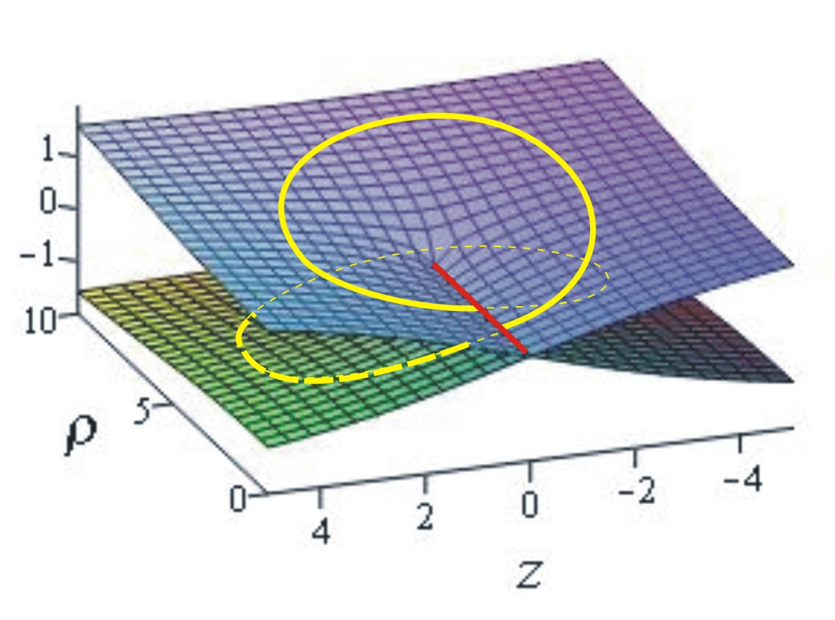
Figure 4: The scalar field $\phi(\rho,z)$ on the manifold $\overline{\cal D}{}_{2}$ corresponding to the single-wormhole spacetime. The segment ${\cal T}=\{\rho\in[0,a],z=0\}$ corresponds to the wormhole’s throat with the radius $a=5$.

The metric function $\nu_{\pm}(\rho,z)$ given by Eq. 19 has been obtained straightforwardly through the coordinate transformation 14 applied to the solution 12. On the other hand, $\nu(\rho,z)$ could be found directly as the line integral 8. Since $\lambda(r)=0$, Eq. 8 reads

$$\nu(\rho,z)=\int_{\cal C}\left[-{\textstyle\frac{1}{2}}\rho(\phi_{,\rho}^{2}-\phi_{,z}^{2})d\rho-\rho\phi_{,\rho}\phi_{,z}dz\right],$$ (22)

where $\cal C$ is an arbitrary path connecting some initial point $(\rho_{0},z_{0})$ and any point $(\rho,z)$ in $\overline{\cal D}{}_{2}$. Note that if $(\rho_{0},z_{0})$ and $(\rho,z)$ are lying in the different charts ${\cal D}_{-}$ and ${\cal D}_{+}$, then the path $\cal C$ should go through the segment $\{\rho\in[0,a],z=0\}$, which corresponds to the wormhole’s throat. The coordinates of the initial point $(\rho_{0},z_{0})$ are determined by the boundary conditions for function $\nu$. Imposing the following boundary conditions

$$\lim\limits_{\rho\to\infty,z\to-\infty}\nu(\rho,z)=0,\quad(\rho,z)\in{\cal D_{+}},$$

substituting $\phi$ from Eq. 21, and integrating, we obtain the expression 19. Finally, the complete solution $\nu(\rho,z)$ defined on $\overline{\cal D}{}_{2}$ is constituted from the separate $\nu_{\pm}(\rho,z)$ as follows

$$\nu(\rho,z)=\left\{\begin{array}[]{ll}\nu_{-}(\rho,z)&\mathrm{if}\ (\rho,z)\in{\cal D}_{-}\\ \nu_{+}(\rho,z)&\mathrm{if}\ (\rho,z)\in{\cal D}_{+}\end{array}\right.$$ (23)

Since $\nu_{-}(\rho,z)$ and $\nu_{+}(\rho,z)$ are given by the same expression 19, a graph of $\nu(\rho,z)$ is represented by two identical sheets topologically glued along the cuts on $\nu_{\pm}(\rho,z)$ with $\rho\in[0,a]$ and $z=0$ (see Fig. 5).

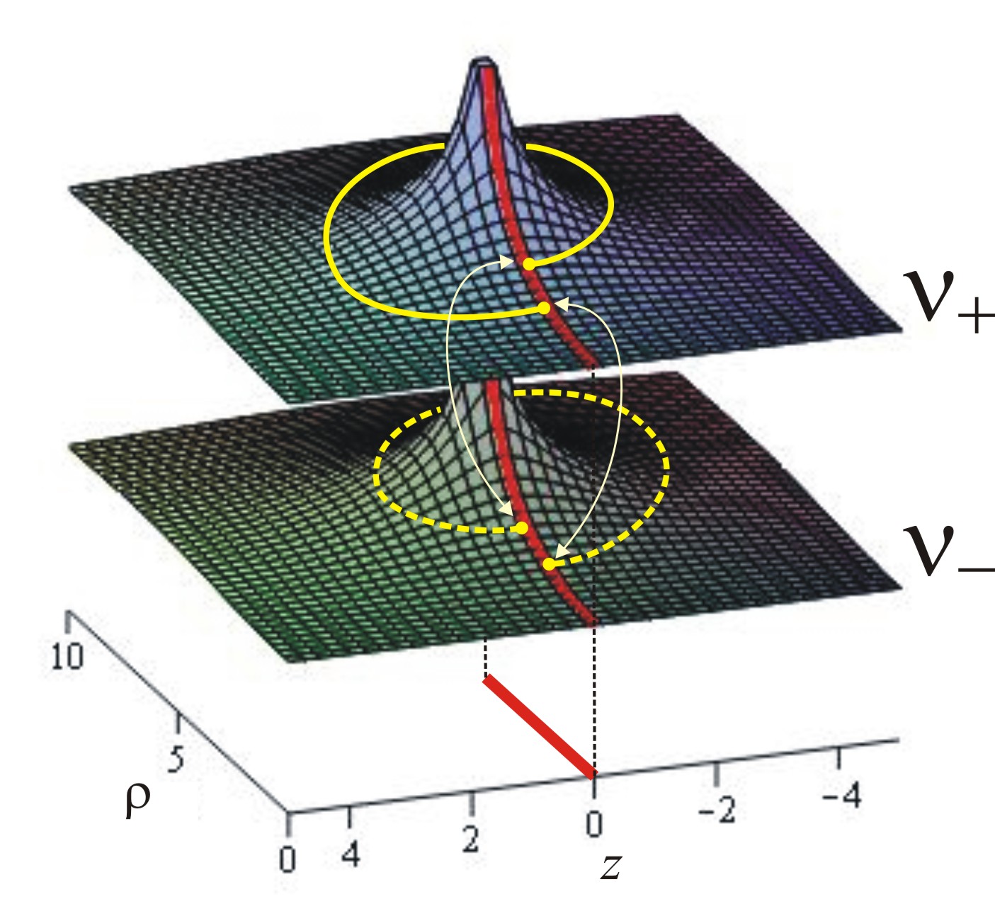
Figure 5: A plot of $\nu(\rho,z)$. It consists of two identical sheets, $\nu_{-}(\rho,z)$ and $\nu_{+}(\rho,z)$, topologically glued along the cuts on $\nu_{\pm}(\rho,z)$ with $\rho\in[0,a]$ and $z=0$.

IV.2 Two wormholes

Now, let us construct a two-wormhole solution. For this aim we remind ourselves that any superposition $c_{1}\phi_{1}+c_{2}\phi_{2}$ of two particular solutions $\phi_{1}$ and $\phi_{2}$ is a solution of the Laplace equation. Moreover, because of the axial symmetry, if $\phi(\rho,z)$ is a solution, then $\phi(\rho,z+\mathrm{const})$ is also a solution of $\Delta\phi=0$, where $\Delta=\frac{1}{\rho}\frac{\partial}{\partial\rho}\left({\rho\frac{\partial}{\partial\rho}}\right)+\frac{\partial^{2}}{\partial z^{2}}$ is the Laplace operator in cylindrical coordinates. Using these properties, we may construct new axially symmetric solutions as a superposition of single-wormhole solutions 20. In particular, the superposition of two solutions reads

$$\phi_{\epsilon_{1}\epsilon_{2}}(\rho,z)=\frac{1}{2}\left[\phi_{\epsilon_{1}}(\rho,z-z_{1};a_{1})+\phi_{\epsilon_{2}}(\rho,z-z_{2};a_{2})\right],$$ (24)

with

$$\phi_{\epsilon_{i}}(\rho,z-z_{i};a_{i})=\epsilon_{i}\sqrt{2}\arctan\left(\frac{R(\rho,z-z_{i})}{a_{i}}\right),$$ (25)

where $i=1,2$, and indices $\epsilon_{i}$ take two values, $+$ or $-$, i.e. $\epsilon_{i}=\pm$. Each particular solution $\phi_{\epsilon_{i}}(\rho,z-z_{i};a_{i})$ describes a single wormhole with the throat of the radius $a_{i}$ located at $z_{i}$. In case $z_{1}=z_{2}=0$ and $a_{1}=a_{2}$, Eq. 24 reproduces the single-wormhole solution 20. As the result, the superposition 24 gives us four new solutions $\phi_{++}$, $\phi_{+-}$, $\phi_{-+}$, and $\phi_{--}$, which could be interpreted as the scalar field in the wormhole spacetime with two throats of radiuses $a_{1}$ and $a_{2}$ located at $z_{1}$ and $z_{2}$, respectively.

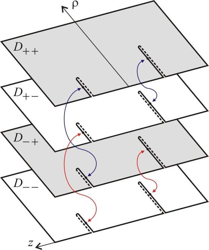
Figure 6: The manifold $\overline{\cal D}{}_{4}$ consists of four identical copies of the half-planes ${\cal D}_{\epsilon_{1}\epsilon_{2}}$ ($\epsilon_{i}=\pm$), which are glued together by the two-sided segments ${\cal T}_{a_{i}}=\{\rho\in[0,a_{i}],z=z_{i}\}$ ($i=1,2$) corresponding to two throats with radii $a_{i}$ located at $z_{i}$.

Note that the domain of $\phi_{\epsilon_{1}\epsilon_{2}}(\rho,z)$ is the same as that of the single-wormhole solutions $\phi_{\epsilon_{i}}(\rho,z-z_{i};a_{i})$, i.e. the half-plane ${\cal D}=[0,\infty)\times(-\infty,\infty)$. The segments ${\cal T}_{a_{i}}=\{\rho\in[0,a_{i}],z=z_{i}\}$ ($i=1,2$) on ${\cal D}$ represent two throats with radii $a_{i}$ located at $z_{i}$, respectively. Graphs of $\phi_{\epsilon_{1}\epsilon_{2}}(\rho,z)$ are shown separately in Fig. 7. It is seen that each of $\phi_{\epsilon_{1}\epsilon_{2}}(\rho,z)$ is not smooth at ${\cal T}_{a_{i}}$. To construct a smooth solution, we consider four identical copies of the half-plane $\cal D$, denoted as ${\cal D}_{\epsilon_{1}\epsilon_{2}}$. On each copy ${\cal D}_{\epsilon_{1}\epsilon_{2}}$ we choose two segments ${\cal T}_{a_{i}}$ ($i=1,2$), and then constitute a new manifold gluing the half-planes ${\cal D}_{\epsilon_{1}\epsilon_{2}}$ along ${\cal T}_{a_{i}}$. The gluing procedure is the following: ${\cal D}_{+\epsilon_{2}}$ and ${\cal D}_{-\epsilon_{2}}$ are glued along the throat ${\cal T}_{a_{1}}$, and ${\cal D}_{\epsilon_{1}+}$ and ${\cal D}_{\epsilon_{1}-}$ are glued along the throat ${\cal T}_{a_{2}}$. The gluing procedure is schematically shown in Fig. 6. As the result of this topological gluing, we obtain a new manifold denoted as $\overline{\cal D}{}_{4}$, consisting of four sheets ${\cal D}_{\epsilon_{1}\epsilon_{2}}$. Note that each of ${\cal D}_{\epsilon_{1}\epsilon_{2}}$ contains an asymptotically flat region $(\rho^{2}+z^{2})^{1/2}\to\infty$, and so $\overline{\cal D}{}_{4}$ represents the spacetime with four asymptotically flat regions connecting by the throats ${\cal T}_{a_{i}}$. It is also worth noticing that the resulting manifold $\overline{\cal D}{}_{4}$ is homeomorphic to a self-crossing four-sheeted Riemann surface.

The complete solution $\phi(\rho,z)$, defined on the whole manifold $\overline{\cal D}{}_{4}$, is constituted from separate $\phi_{\epsilon_{1}\epsilon_{2}}(\rho,z)$ as follows:

$$\phi(\rho,z)=\bigcup_{\epsilon_{1}\epsilon_{2}}\big{\{}\phi_{\epsilon_{1}\epsilon_{2}}(\rho,z)~{}\textrm{if}~{}(\rho,z)\in{\cal D}_{\epsilon_{1}\epsilon_{2}}\big{\}}.$$ (26)

To argue that $\phi(\rho,z)$ is a smooth function on $\overline{\cal D}{}_{4}$, we note that the single-wormhole solutions $\phi_{+}(\rho,z-z_{i};a_{i})$ and $\phi_{-}(\rho,z-z_{i};a_{i})$ are smoothly matched at the corresponding throat ${\cal T}_{a_{i}}=\{\rho\in[0,a_{i}],z=z_{i}\}$. A plot of $\phi(\rho,z)$ is shown in Fig. 8.

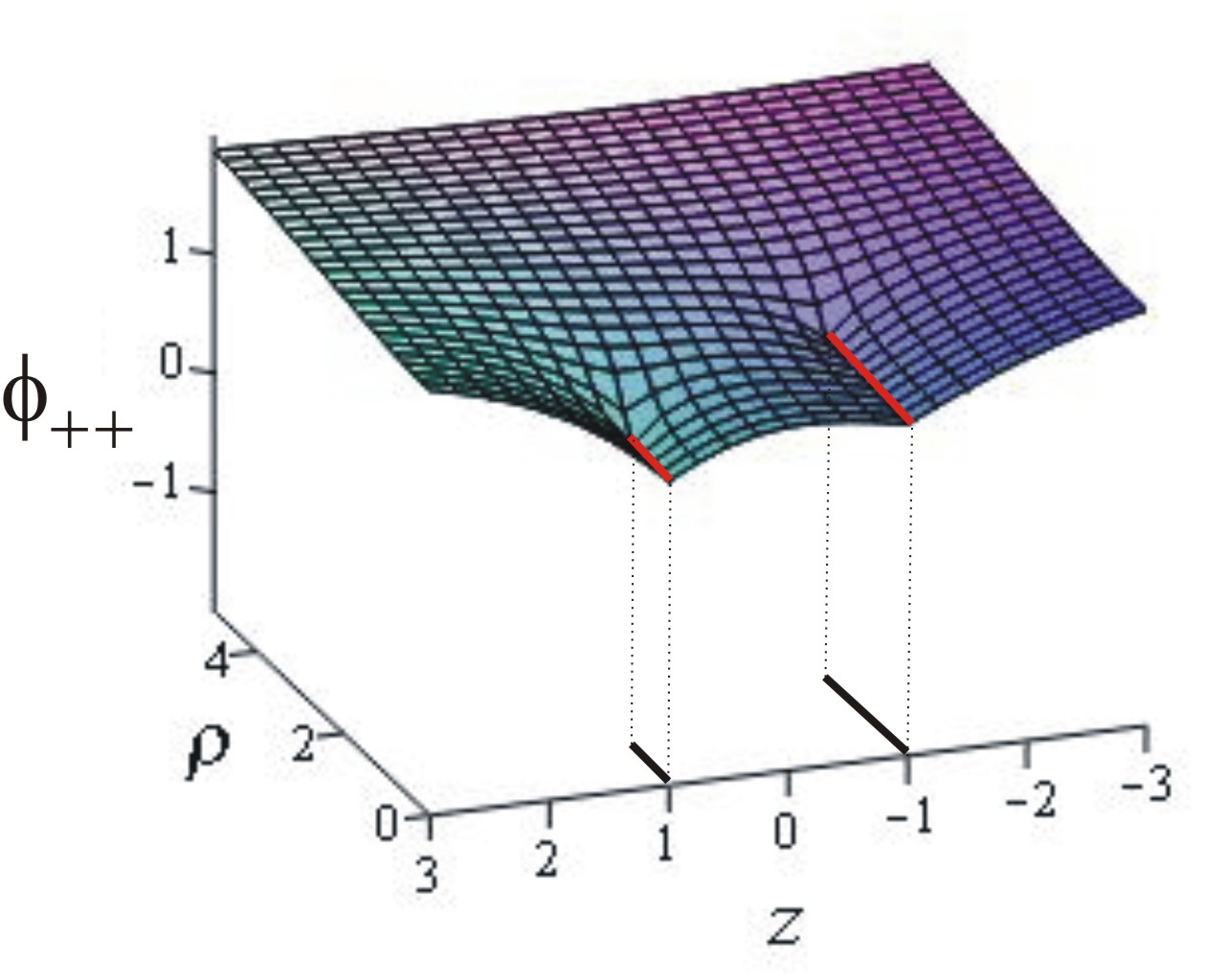
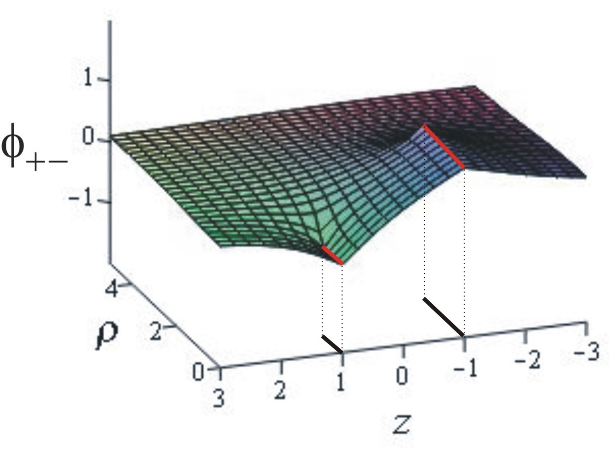
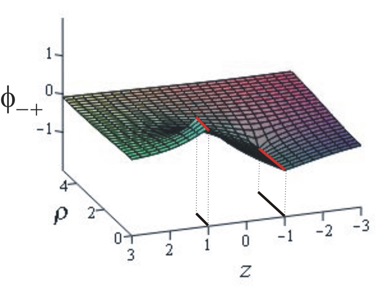
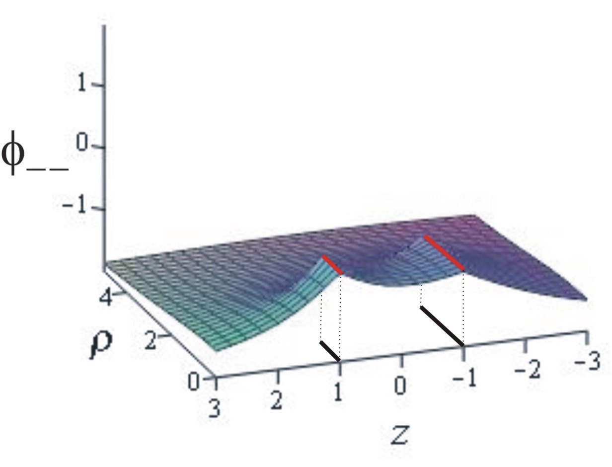
Figure 7: The plot represents separate solutions $\phi_{\epsilon_{1}\epsilon_{2}}(\rho,z)$ on half-planes ${\cal D}_{\epsilon_{1}\epsilon_{2}}$. Here $a_{1}=1$, $a_{2}=2$, and $z_{1}=1$, $z_{2}=-1$.

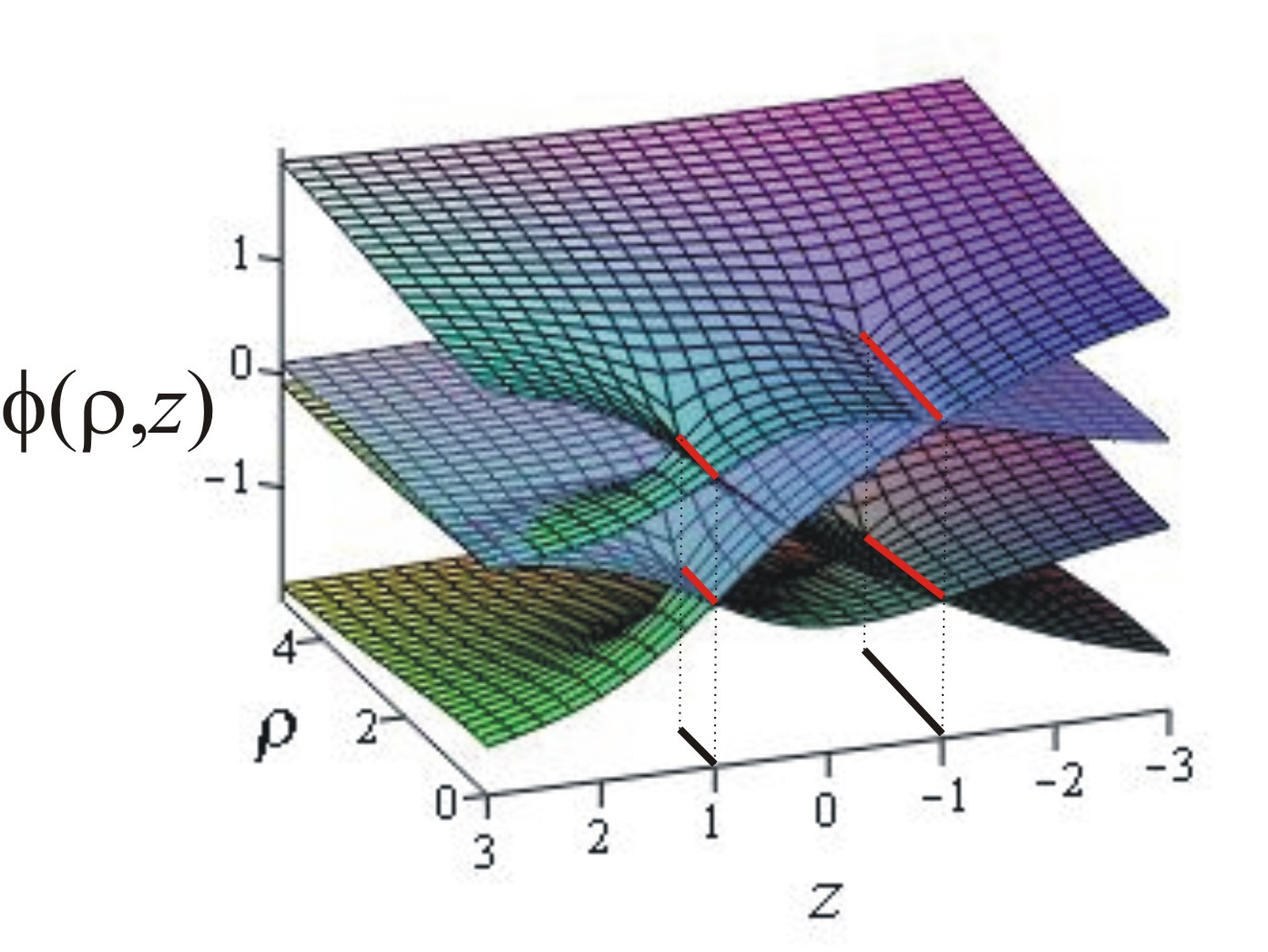
Figure 8: The scalar field $\phi(\rho,z)$ on the manifold $\overline{\cal D}{}_{2^{2}}$ which possesses $2^{2}$ asymptotically flat regions and corresponds to the two-wormhole spacetime. Segments ${\cal T}_{a_{i}}=\{\rho\in[0,a_{i}],z_{i}\}$ $(i=1,2)$ correspond to the wormhole’s throats with the radiuses $a_{1}=1$, $a_{2}=2$, and the positions $z_{1}=1$, $z_{2}=-1$.

The function $\nu(\rho,z)$ could be found as the line integral

$$\nu(\rho,z)=\int_{\cal C}\left[-{\textstyle\frac{1}{2}}\rho(\phi_{,\rho}^{2}-\phi_{,z}^{2})d\rho-\rho\phi_{,\rho}\phi_{,z}dz\right],$$

where $\cal C$ is an arbitrary path connecting some initial point $(\rho_{0},z_{0})$ and any point $(\rho,z)$ in $\overline{\cal D}{}_{4}$. Note that if $(\rho_{0},z_{0})$ and $(\rho,z)$ are lying in different charts ${\cal D}_{\epsilon_{1}\epsilon_{2}}$, then the path $\cal C$ should pass through some throats ${\cal T}_{a_{i}}$. Coordinates of the initial point $(\rho_{0},z_{0})$ are determined by boundary conditions for the function $\nu$. Imposing the following boundary conditions

$$\lim\limits_{\rho\to\infty,z\to-\infty}\nu(\rho,z)=0,\quad(\rho,z)\in{\cal D_{++}},$$

substituting $\phi$ from Eq. 26, and integrating, we can obtain the set of functions $\nu_{\epsilon_{1}\epsilon_{2}}(\rho,z)$ defined on ${\cal D}_{\epsilon_{1}\epsilon_{2}}$, respectively. Finally, the complete solution $\nu(\rho,z)$ defined on $\overline{\cal D}{}_{4}$ is constituted from the separate $\nu_{\epsilon_{1}\epsilon_{2}}(\rho,z)$ as follows

$$\nu(\rho,z)=\bigcup_{\epsilon_{1},\epsilon_{2}}\left\{\nu_{\epsilon_{1}\epsilon_{2}}(\rho,z)~{}\textrm{if }~{}(\rho,z)\in{\cal D}_{\epsilon_{1}\epsilon_{2}}\right\}.$$ (27)

IV.3 $N$ wormholes

A multi-wormhole solution could be constructed analogously to the two-wormhole one. For this aim we consider $2^{N}$ different superpositions of $N$ single-wormhole solutions:

$$\phi_{\epsilon_{1}\epsilon_{2}\dots\epsilon_{N}}(\rho,z)=\frac{1}{N}\sum_{i=1}^{N}\phi_{\epsilon_{i}}(\rho,z-z_{i};a_{i}),$$ (28)

where $i=1,2,\dots,N$, and $\epsilon_{i}$ is an index which stands on the $i$th position and takes two values, $+$ or $-$, i.e. $\epsilon_{i}=\pm$. Each of $\phi_{\epsilon_{1}\epsilon_{2}\dots\epsilon_{N}}(\rho,z)$ is defined on the half-plane ${\cal D}=[0,\infty)\times(-\infty,\infty)$. Consider $2^{N}$ identical copies of $\cal D$, denoted as ${\cal D}_{\epsilon_{1}\epsilon_{2}\dots\epsilon_{N}}$, and then construct a new manifold $\overline{\cal D}{}_{2^{N}}$ gluing the half-planes ${\cal D}_{\epsilon_{1}\epsilon_{2}\dots\epsilon_{N}}$. The gluing procedure is the following: the charts ${\cal D}_{\epsilon_{1}\cdots\{\epsilon_{k}=+\}\cdots\epsilon_{N}}$ and ${\cal D}_{\epsilon_{1}\cdots\{\epsilon_{k}=-\}\cdots\epsilon_{N}}$ are glued along the $k$th segment $\{\rho\in[0,a_{k}],z=z_{k}\}$.

As the result of this topological gluing, we obtain a new manifold $\overline{\cal D}{}_{2^{N}}$, consisting of $2^{N}$ sheets ${\cal D}_{\epsilon_{1}\epsilon_{2}\dots\epsilon_{N}}$. Each of ${\cal D}_{\epsilon_{1}\epsilon_{2}\dots\epsilon_{N}}$ contains an asymptotically flat region $(\rho^{2}+z^{2})^{1/2}\to\infty$, and so $\overline{\cal D}{}_{2^{N}}$ represents the spacetime with $2^{N}$ asymptotically flat regions connecting by the throats ${\cal T}_{a_{i}}$. It is also worth noticing that the resulting manifold $\overline{\cal D}{}_{2^{N}}$ is homeomorphic to a self-crossing $2^{N}$-sheeted Riemann surface.

The complete solution $\phi(\rho,z)$, defined on the whole manifold $\overline{\cal D}{}_{2^{N}}$, is constituted from separate $\phi_{\epsilon_{1}\epsilon_{2}\dots\epsilon_{N}}(\rho,z)$ as follows:

$$\phi(\rho,z)=\bigcup_{\epsilon_{1}\epsilon_{2}\dots\epsilon_{N}}\big{\{}\phi_{\epsilon_{1}\epsilon_{2}\dots\epsilon_{N}}(\rho,z)~{}\textrm{if }~{}(\rho,z)\in{\cal D}_{\epsilon_{1}\epsilon_{2}\dots\epsilon_{N}}\big{\}}.$$ (29)

The metric function $\nu(\rho,z)$ is found as the line integral

$$\nu(\rho,z)=\int_{\cal C}\left[-{\textstyle\frac{1}{2}}\rho(\phi_{,\rho}^{2}-\phi_{,z}^{2})d\rho-\rho\phi_{,\rho}\phi_{,z}dz\right],$$

where $\phi$ is given by Eq. 29, and $\cal C$ is an arbitrary path connecting some initial point $(\rho_{0},z_{0})$ and any point $(\rho,z)$ in $\overline{\cal D}{}_{2^{N}}$.

As an illustration of a multi-wormhole configuration with $N>2$, in Fig. 9 we depict the scalar field in the wormhole spacetime $\overline{\cal D}{}_{2^{3}}$ with $2^{3}$ asymptotically flat regions connecting by the three throats.

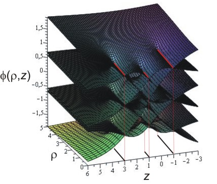
Figure 9: The scalar field $\phi(\rho,z)$ on the manifold $\overline{\cal D}{}_{2^{3}}$ which possesses $2^{3}$ asymptotically flat regions and corresponds to the three-wormhole spacetime. Segments ${\cal T}_{a_{i}}=\{\rho\in[0,a_{i}],z_{i}\}$ $(i=1,2,3)$ correspond to the wormhole’s throats with the radiuses $a_{1}=1$, $a_{2}=1.5$, $a_{3}=2$, and the positions $z_{1}=1$, $z_{2}=3$, $z_{3}=-1$.

V Conclusions

Many years ago, in 1921 Bach and Weyl BachWeyl derived the method of superposition to construct new axially symmetric vacuum solutions of General Relativity and obtained the famous solution interpreted as equilibrium configurations of a pair of Schwarzschild black holes. In this paper we have extended the Bach-Weyl approach to non-vacuum configurations with massless scalar fields. Considering phantom scalar fields with the negative kinetic energy, we have constructed multi-wormhole solutions describing an axially symmetric superposition of $N$ wormholes. Let us enumerate basic properties of the obtained solutions.

• The most unusual property is that the multi-wormhole spacetime has a complicated topological structure. Namely, in the spacetime there exist $2^{N}$ asymptotically flat regions connected by throats, so that the resulting spacetime manifold is homeomorphic to a self-crossing $2^{N}$-sheeted Riemann surface.

• The spacetime of multi-wormholes is everywhere regular and has no event horizons. This feature drastically tells the multi-wormhole configuration from other axially symmetric vacuum solutions. As is known, all static solutions, representing the superposition of two or more axially symmetric bodies, inevitably contain gravitationally inert singular structures, ‘struts’ and ‘membranes’, that keep the two bodies apart making a stable configuration. This is an expected “price to pay” for the stationarity. However, the multi-wormholes are static without any singular struts. Instead, the stationarity of the multi-wormhole configuration is provided by the phantom scalar field with the negative kinetic energy. Phantom scalars represent exotic matter violating the null energy condition. Therefore, now an “exoticism” of the matter source supporting the multi-wormholes is a price for the stationarity.

References

- (1) J. Droste, Versl. K. Akad. Wet. Amsterdam, 19, 447-455 (1916).
- (2) W. De Sitter, Mon. Not. R. Astr. Soc. 76, 699-728 (1916); 77, 155-184 (1916).
- (3) H.A. Lorentz and J. Droste, Versl. K. Akad. Wet. Amsterdam 26, 392 (1917); and 26, 649 (1917).
- (4) T. Levi-Civita, Am. J. Math. 59, 9-22 (1937); Am. J. Math. 59, 225-234 (1937); Le problème des corps en relativité générale, Mémorial des Sciences Mathématiques 116 (Gauthier-Villars, Paris, 1950).
- (5) A. Einstein, L. Infeld and B. Hoffmann, Ann. Math. 39, 65 (1938).
- (6) T. Damour, The general relativistic two body problem, arXiv:1312.3505.
- (7) L. Blanchet, Post-Newtonian theory and the two-body problem, arXiv:0907.3596.
- (8) Weyl H 1917 Zur gravitationstheorie Ann. Phys., Lpz. 54 117-45 Weyl H 1919 Zur gravitationstheorie Ann. Phys., Lpz. 59 185-8
- (9) Levi-Civita T 1917 Realtá fisica di alcuni spazi normalidel Bianchi Rendiconti della Reale Accademia del Lincei 26 519-531 Levi-Civita T 1919 einsteiniana in campi newtoniani. IX: l’analogo del potenziale logaritmico Rendiconti della Reale Accademia del Lincei 28 101-109
- (10) R. Bach and H. Weyl, Neue Lösungen der Einsteinschen Gravitationsgleichungen, Mathematische Zeitschrift 13, 132-145 (1921).
- (11) Chazy M 1924 Sur le champ de gravitation de deux masses fixes dans la theorie de la relativit? e? Bull. Soc. Math. France 52 17-38.
- (12) Curzon H 1924 Cylindrical solutions of Einstein s gravitation equations Proc. London Math. Soc. 23 477-80
- (13) Chou P 1931 The gravitational field of a body with rotational symmetry in Einstein?s theory of gravitation J. Math. 53 289-308
- (14) Synge J 1960 Relativity: The General Theory (Amsterdam: North-Holland), p. 314.
- (15) Bondi H 1957 Rev. Mod. Phys. 29 423
- (16) W. Israel, K. A. Khan, Nuovo Cimento, 33, 331 (1964).
- (17) Letelier P S and Oliveira S R 1987 Exact self-gravitating disks and rings: a solitonic approach J. Math. Phys. 28 165-70
- (18) Letelier P S and Oliveira S R 1988 Superposition of Weyl solutions: cosmic strings and membranes Class. Quantum Grav. 5 L47-51
- (19) Einstein A and Rosen N 1936 Two-body problem in general relativity theory Phys. Rev. 49 404-5
- (20) Cooperstock F 1974 Axially symmetric two-body problem in general relativity Phys. Rev. D 10 3171 80
- (21) Tomimatsu A and Kihara M 1982 Conditions for regularity on the symmetry axis in a superposition of two Kerr-NUT solutions Prog. Theor. Phys. 67 1406-14
- (22) Yamazaki M 1982 On the Kramer-Neugebauer spinning masses solutions Prog. Theor. Phys. 69 503-15
- (23) Schleifer N 1985 Condition of elementary flatness and the two-particle Curzon solution Phys. Lett. 112A 204-8
- (24) Morris M S and Thorne K S 1988 American Journal of Physics 56, 395
- (25) Visser M 1995 Lorentzian Wormholes: from Einstein to Hawking (Woodbury: American Institute of Physics)
- (26) Hochberg D and Visser M 1997 Phys. Rev. D 56 4745
- (27) Hochberg D and Visser M 1998 Phys. Rev. D 58 044021
- (28) H. Ellis, J. Math. Phys. 14, 104 (1973).
- (29) K.A. Bronnikov, Acta Phys. Polonica B 4, 251 (1973).
- (30) S.V. Sushkov, S.-W. Kim, Gen. Rel. Grav. 36, 1671 (2004).