An Anderson-like model of the QCD chiral transition

Abstract

We study the problems of chiral symmetry breaking and eigenmode localisation in finite-temperature QCD by looking at the lattice Dirac operator as a random Hamiltonian. We recast the staggered Dirac operator into an unconventional three-dimensional Anderson Hamiltonian (“Dirac-Anderson Hamiltonian”) carrying internal degrees of freedom, with disorder provided by the fluctuations of the gauge links. In this framework, we identify the features relevant to chiral symmetry restoration and localisation of the low-lying Dirac eigenmodes in the ordering of the local Polyakov lines, and in the related correlation between spatial links across time slices, thus tying the two phenomena to the deconfinement transition. We then build a toy model based on QCD and on the Dirac-Anderson approach, replacing the Polyakov lines with spin variables and simplifying the dynamics of the spatial gauge links, but preserving the above-mentioned relevant dynamical features. Our toy model successfully reproduces the main features of the QCD spectrum and of the Dirac eigenmodes concerning chiral symmetry breaking and localisation, both in the ordered (deconfined) and disordered (confined) phases. Moreover, it allows us to study separately the roles played in the two phenomena by the diagonal and the off-diagonal terms of the Dirac-Anderson Hamiltonian. Our results support our expectation that chiral symmetry restoration and localisation of the low modes are closely related, and that both are triggered by the deconfinement transition.

1 Introduction

The low end of the spectrum of the Euclidean Dirac operator plays an important role in determining the properties of hadronic matter in Quantum Chromodynamics (QCD). In particular, the spectral density around the origin is closely tied to the fate of chiral symmetry, and entirely determines it in the chiral limit BC . It is thus not surprising that the low end of the Dirac spectrum behaves differently in the broken and in the restored phase. The most important difference is obviously that while in the broken phase eigenvalues accumulate around the origin, in the restored phase the spectral density vanishes there. Besides this, or perhaps as a consequence, the low-lying eigenmodes display different localisation properties and statistical behaviour.

Numerical simulations of QCD on the lattice have shown that the low-lying Dirac eigenmodes, while delocalised on the entire lattice volume at low temperature VWrev ; deF , become spatially localised at high temperature GGO ; GGO2 ; KGT ; KP ; BKS ; KP2 ; feri ; crit ; Cossu:2014aua ; Cossu:2016scb , above the chiral crossover Aoki:2005vt ; Borsanyi:2010cj . Although most of the studies of this phenomenon have been carried out using the staggered discretisation of the Dirac operator GGO ; GGO2 ; KP ; BKS ; KP2 ; feri ; crit , there is also evidence in simulations with overlap KGT ; BKS and domain wall Cossu:2014aua ; Cossu:2016scb fermions. Let us summarise the current knowledge about it (see Ref. Giordano:2014qna for a review), focussing on the case of the staggered operator. In this case the eigenvalues $i\lambda$ are purely imaginary and the spectrum is symmetric with respect to zero, so it suffices to discuss $\lambda\geq 0$. Above the QCD crossover temperature, $T_{c}$, the low-lying quark eigenmodes are spatially localised on the scale of the inverse temperature, for eigenvalues below a critical point in the spectrum, $\lambda_{c}$. Eigenmodes above $\lambda_{c}$, on the other hand, extend throughout the whole system. The position of the critical point depends on the temperature, $\lambda_{c}=\lambda_{c}(T)$, and it extrapolates to $\lambda_{c}=0$ at a temperature compatible with $T_{c}$, as determined from thermodynamic observables Aoki:2005vt ; Borsanyi:2010cj . This strongly suggests that the appearance of localised modes is related to the deconfinement/chiral transition. Further evidence in this respect comes from simulations of quenched QCD with $N_{c}=3$ GGO2 and $N_{c}=2$ KP colours, and from the study of unimproved staggered fermions for temporal extension $N_{T}=4$ in lattice units unimproved reported in Ref. GKKP : both models display a genuine deconfinement/chiral phase transition, accompanied by the appearance of localised modes.

As we mentioned above, the different localisation properties of the low-lying modes in the low and high temperature phases of QCD come along with different statistical properties. At low temperature there is clear evidence that the eigenvalues obey the Wigner–Dyson statistics predicted by Random Matrix Theory (RMT) VWrev . At high temperature, on the other hand, the localised modes at the low end of the spectrum fluctuate independently, thus obeying Poisson statistics, while the delocalised eigenmodes higher up in the spectrum, above $\lambda_{c}$, obey again the predictions of RMT KP ; BKS ; KP2 ; feri ; crit . This allows one to study the localisation/delocalisation transition by looking at the spectral statistics.

In Ref. crit the transition in the spectrum from localised to delocalised modes was shown to be a true second-order phase transition, analogous to the metal-insulator transition in the Anderson model Anderson58 ; LR ; EM , which describes non-interacting electrons in a disordered crystal. By studying the corresponding transition in the statistical properties of the spectrum, the correlation-length critical exponent was found to be compatible with that of the 3D unitary Anderson model nu_unitary . “Unitary” refers here to the symmetry class of the model in the RMT classification of random matrix ensembles Mehta , and the staggered Dirac operator also belongs to this class VWrev . This result for the critical exponent has been recently confirmed by a study of the multifractal properties of the eigenmodes at criticality UGPKV . In the same paper it was also found that the multifractal exponents of the critical eigenmodes in QCD are compatible with those of the 3D unitary Anderson model UV , which further supports that the delocalisation transitions in the two models belong to the same universality class.

The result about the universality class of the delocalisation transition in the high-temperature Dirac spectrum of QCD is quite surprising. As a statistical model, lattice QCD at finite temperature is four-dimensional (although anisotropic), while the 3D unitary Anderson model is, well, three-dimensional. Moreover, the Hamiltonian of the 3D unitary Anderson model consists of a diagonal, on-site random potential, and of nearest-neighbour hopping terms with fixed and uniform strength (and random phases). The staggered Dirac operator, on the other hand, consists entirely of off-diagonal nearest-neighbour hopping terms, depending on the gauge transporter on the corresponding lattice link, and it is known from the condensed-matter literature that off-diagonal noise is much less effective in inducing localisation, with a large amount of disorder required to this end offdiag ; offdiag2 ; GGC .

A possible explanation of the fact that the two models share the same universality class has been proposed in Ref. GKP , elaborating on a previous proposal made in Ref. BKS for the mechanism leading to localisation. The main idea is that high-temperature QCD effectively contains a source of 3D on-site disorder, which consists of the phases of the local Polyakov line at a given spatial point. Above $T_{c}$ the Polyakov lines get ordered along the identity, with local fluctuations away from it. The Polyakov line phases affect the quark eigenmodes through effective boundary conditions in the temporal direction, and make favourable for the quark wave function to “live” on the “islands” of unordered Polyakov lines. As a random matrix model, the Dirac operator in high-temperature QCD is thus effectively 3D with diagonal noise. Support to the viability of this mechanism was obtained in Ref. BKS by studying the correlation of the Dirac eigenfunctions with the fluctuations of the Polyakov loop on $SU(2)$ gauge configurations. In Ref. GKP we looked for a different kind of evidence: we constructed, and studied numerically, a QCD-inspired toy model which should display localisation precisely through the proposed mechanism, but in a much simplified setting. This “Ising-Anderson” model is essentially obtained by removing the temporal direction, thus working in three-dimensional space (i.e., a single time slice), and by mimicking the effect of the Polyakov lines on the quark wave functions with a (continuous) spin model of the Ising class in the ordered phase, used to generate the appropriate diagonal noise. This model adequately reproduces the main features of localisation, in particular their qualitative dependence on the amount of “islands” of “wrong” spins in the “sea” of ordered spins, as expected from the proposed explanation.

Although the Ising-Anderson model of Ref. GKP provides a satisfactory qualitative description of localisation in the high-temperature phase of QCD, it fails completely at describing the low-temperature phase. Indeed, simulations in the disordered phase of the underlying Ising model (not reported in Ref. GKP , but see Section 4 below for similar results) fail to reproduce the most distinctive feature of the Dirac spectrum at low temperature, namely the presence of a nonzero spectral density around the origin, which leads to the spontaneous breaking of chiral symmetry BC . Instead, a sharp gap separates the lowest eigenvalues from the origin, both when the underlying spin model is in the ordered phase, and when it is in the disordered phase. While in the former case this is in rough qualitative agreement with the small density of near-zero modes in QCD at high temperature, in the latter case this is at odds with the existing numerical results. On the other hand, the mechanism through which the Polyakov lines affect the quark wave functions, i.e., the effective boundary conditions, is in principle at work at all temperatures, and only the presence of order in the (relevant) Polyakov-line configurations, or lack thereof, distinguish the two phases. As we have already said above, the effectiveness of the “sea/islands” mechanism devised in Refs. BKS ; GKP can explain the presence of localised modes at high temperature. For the explanation to be complete, the ineffectiveness of this same mechanism should also explain the absence of localised modes at low temperatures. This requirement is even more compelling in light of the apparently very close relation between localisation and the QCD crossover: the reason for the ineffectiveness of the mechanism at low temperature is likely to be also the reason for the finiteness of the spectral density at the origin.

Above we said that the effective boundary conditions are in principle at work at all temperatures but, as a matter of fact, they turn out to be irrelevant at low temperatures, where QCD looks “effectively 4D”. The ineffectiveness of the boundary conditions at low temperatures clearly entails the ineffectiveness of the “sea/islands” mechanism for localisation, and so it may seem hopeless to try to give a simultaneous description of the QCD crossover and of the appearance of localised modes by means of a 3D model. Still, one can technically treat the quark degrees of freedom along the compactified temporal direction as internal degrees of freedom of a quark living in 3D space. In doing this, one can in principle make the temporal extent of the lattice as small as possible in lattice units, thus reducing the amount of such internal degrees of freedom to a minimum. In this setting, whether the system is effectively 3D or 4D becomes a question about the correlation among the internal degrees of freedom. For this question to make any sense at all, the number of such degrees of freedom has clearly to be at least two. Perhaps a more natural way of phrasing this is in terms of the temporal correlation length, and the minimal number of time slices for which one can ask if they are strongly correlated is obviously two.

With this (in hindsight rather obvious) insight, our purpose in this paper is to build a refined toy model, aimed at describing the (supposedly) simultaneous appearance of localised modes and recovery of chiral symmetry, as signalled by the vanishing of the spectral density at the origin. The motivation is twofold. On the one hand, we want to implement the “sea/islands” mechanism in a model that reproduces QCD more faithfully (at the qualitative level), in order to make the case of Refs. BKS ; GKP stronger. On the other hand, we want to investigate the connection between localisation and the deconfinement/chiral transition in a simple and controllable setting. This could also lead to some insight into the chiral transition, and into its relation to deconfinement, from the point of view of the QCD Dirac operator as a random matrix model, independently of the issue of localisation. Indeed, since localisation of the low modes and restoration of chiral symmetry take place together, and this happens near the deconfinement transition, it is very likely that they are both triggered by the ordering of the gauge configurations, so that some mechanism could be devised which would explain both phenomena.

Here is the plan of the paper. Before building the toy model, in Section 2 we cast the staggered Dirac operator into a three-dimensional Hamiltonian, with internal degrees of freedom corresponding to colour and to the lattice temporal momenta. In this way the connection with Anderson-type models is made transparent. In Section 3 we write down explicitly our toy model, which we study numerically in Section 4. Finally, in Section 5 we discuss our results, state our conclusions and comment about future prospects. Some technical details are discussed in Appendix A.

2 Staggered Dirac operator as a random matrix model

In this Section we recast the Dirac operator in lattice QCD, ${\not{D}}$, as the Hamiltonian of an unconventional three-dimensional Anderson model. We work here with the staggered Dirac operator for simplicity.

The basic idea is to split the “Hamiltonian” $H=-i{\not{D}}$ into a “free” and an “interaction” part, $H=H_{0}+H_{I}$, and then work in the basis of the “unperturbed” eigenvectors of $H_{0}$. At finite temperature the temporal direction is compactified and therefore singled out, and so the physically most sensible choice is to identify the free Hamiltonian with the temporal hoppings. This leaves the spatial hoppings as the (spatially isotropic) interaction part. We thus define

$$H_{0}: (H_{0})_{xx^{\prime}} =\frac{\eta_{4}(\vec{x})}{2i}\left\{U_{4}(t,\vec{x})\delta_{t+1,t^{\prime}}-U_{-4}(t,\vec{x})\delta_{t-1,t^{\prime}}\right\}\delta_{\vec{x}\vec{x}{}^{\prime}}\,,$$  temporal hoppings, (1)

$$H_{I}: (H_{I})_{xx^{\prime}} =\sum_{j=1}^{3}\frac{\eta_{j}(\vec{x})}{2i}\left\{U_{j}(t,\vec{x})\delta_{\vec{x}+\hat{\jmath},\vec{x}{}^{\prime}}-U_{-j}(t,x)\delta_{\vec{x}-\hat{\jmath},\vec{x}{}^{\prime}}\right\}\delta_{tt^{\prime}}\,,$$  spatial hoppings,

where $x=(t,\vec{x})$ with $t$ the Euclidean “time”, $0\leq t\leq N_{T}-1$, and the staggered phases $\eta_{\mu}(\vec{x})$ are given by

$$\eta_{\mu}(\vec{x})=(-1)^{\left(\sum_{\nu=1}^{\mu}x_{\nu}\right)-x_{\mu}}\,,$$ (2)

and depend only on the spatial coordinates, $0\leq x_{i}\leq L-1$, $i=1,2,3$. Both $N_{T}$ and $L$ must be even. We take the gauge links $U_{\mu}(t,\vec{x})\in SU(N_{c})$ for generality, and denote the backward links by $U_{-4}(t,\vec{x})\equiv U^{\dagger}_{4}(t-1,\vec{x})$ and $U_{-j}(t,\vec{x})\equiv U^{\dagger}_{j}(t,\vec{x}-\hat{\jmath})$, $j=1,2,3$. Periodic boundary conditions are understood for the gauge links, while on the quark wavefunctions antiperiodic boundary conditions in the temporal direction, and periodic boundary conditions in the spatial directions, are imposed. In Eq. (1) colour indices are suppressed.

The eigenvectors of $H_{0}$ are easily determined. To this end, let us define the following gauge transporters in the temporal direction,

$$P_{0}(\vec{x})\equiv\mathbf{1}\,,\qquad P_{t+1}(\vec{x})\equiv P_{t}(\vec{x})U_{4}(t,\vec{x})\,,~{}0\leq t\leq N_{T}-1\,,$$ (3)

with $P_{N_{T}}(\vec{x})=P(\vec{x})$ the usual (untraced) Polyakov line starting at $t=0$ and winding around the temporal direction. Let furthermore $\varphi_{a}(\vec{x})$ be the (ortho)normalised eigenvectors of $P(\vec{x})$,

$$P(\vec{x})\varphi_{a}(\vec{x})=e^{i\phi_{a}(\vec{x})}\varphi_{a}(\vec{x})\,,\qquad\varphi_{a}^{\dagger}(\vec{x})\varphi_{b}(\vec{x})=\delta_{ab}\,.$$ (4)

Here $\vec{x}$ runs over the whole 3-volume, $a=1,\ldots,N_{c}$ with $N_{c}$ the number of colours, and each $\varphi_{a}$ has $N_{c}$ colour components, $(\varphi_{a})_{i}$. The eigenvalues $e^{i\phi_{a}(\vec{x})}$ have unit absolute value and satisfy $\prod_{a}e^{i\phi_{a}(\vec{x})}=1$. The eigenvectors of the Polyakov line can be used to build the eigenvectors $\psi_{0}^{\vec{x}\,a\,k}$ of $H_{0}$. These are localised on a single spatial point, $\vec{x}$, have a well-defined temporal momentum, $k$, and carry a colour quantum number, $a$, and read (in the coordinate basis)

$$\psi_{0}^{\vec{x}\,a\,k}(t,\vec{y})=\frac{1}{\sqrt{N_{T}}}\,\delta_{\vec{x}\vec{y}}\,e^{i\omega_{ak}(\vec{x})t}\,P_{t}^{\dagger}(\vec{x})\varphi_{a}(\vec{x})\,,$$ (5)

with colour- and space-dependent effective Matsubara frequencies, $\omega_{ak}(\vec{x})$,

$$\omega_{ak}(\vec{x})={\textstyle\frac{1}{N_{T}}}(\pi+\phi_{a}(\vec{x})+2\pi k)\,,\qquad k=0,1,\ldots,N_{T}-1\,.$$ (6)

The form of $\omega_{ak}(\vec{x})$ results from imposing temporal antiperiodic boundary conditions on the fermions, and from the presence of nontrivial Polyakov lines which modify the free-field result. The $\psi_{0}^{\vec{x}\,a\,k}$ are eigenvectors of $H_{0}$ with “unperturbed” eigenvalues $\lambda_{0}^{\vec{x}\,a\,k}$ given by

$$\lambda_{0}^{\vec{x}\,a\,k}=\eta_{4}(\vec{x})\sin\omega_{ak}(\vec{x})\,.$$ (7)

Notice that

$$\sin\omega_{ak^{\prime}}(\vec{x})=-\sin\omega_{ak}(\vec{x})~{}~{}\text{if}~{}~{}k^{\prime}=\textstyle\left(\frac{N_{T}}{2}+k\right)_{N_{T}}\,,$$ (8)

where we have denoted $\left(a+b\right)_{N_{T}}\equiv a+b\mod N_{T}$. In the basis $\{\psi_{0}^{\vec{x}\,a\,k}\}$, the operator $H_{I}$ has vanishing diagonal elements, and only nearest-neighbour hopping terms (i.e., connecting eigenvectors localised on nearest-neighbour sites),

$${[H_{I}]}_{\vec{x}\,a\,k,\vec{y}\,b\,l} =\sum_{j=1}^{3}\delta_{\vec{x}+\hat{\jmath},\vec{y}}[H_{I}]_{\vec{x}\,a\,k,\vec{x}+\hat{\jmath}\,b\,l}+\delta_{\vec{x}-\hat{\jmath},\vec{y}}[H_{I}]_{\vec{x}\,a\,k,\vec{x}-\hat{\jmath}\,b\,l}\,,$$ (9)

$$[H_{I}]_{\vec{x}\,a\,k,\vec{x}\pm\hat{\jmath}\,b\,l} =\pm\frac{\eta_{j}(\vec{x})}{2i}\frac{1}{N_{T}}\sum_{t=0}^{N_{T}-1}e^{i[\omega_{bl}(\vec{x}\pm\hat{\jmath})-\omega_{ak}(\vec{x})]t}\left[{U}^{\rm(td)}_{\pm j}(t,\vec{x})\right]_{ab}\,,$$

where

$$\left[{U}^{\rm(td)}_{\pm j}(t,\vec{x})\right]_{ab}=\varphi_{a}^{\dagger}(\vec{x})P_{t}(\vec{x})U_{\pm j}(t,\vec{x})P_{t}^{\dagger}(\vec{x}\pm\hat{\jmath})\varphi_{b}(\vec{x}\pm\hat{\jmath})\,.$$ (10)

Notice that ${U}^{\rm(td)}_{\pm j}(t,\vec{x})$ is just the usual link variable in the temporal diagonal gauge, i.e., the temporal gauge where the Polyakov lines have been diagonalised.

The full Hamiltonian in the basis of “unperturbed” eigenvectors, $\{\psi_{0}^{\vec{x}\,a\,k}\}$, will be denoted by ${\cal H}$, and it carries space, colour, and temporal-momentum indices, $[{\cal H}(\vec{x},\vec{y})]_{ak,bl}$. Suppressing the latter two indices, we will write

$${\cal H}(\vec{x},\vec{y}) ={\cal D}(\vec{x},\vec{y})+\sum_{j=1}^{3}\frac{\eta_{j}(\vec{x})}{2i}\left\{{\cal V}_{+j}(\vec{x},\vec{y})-{\cal V}_{-j}(\vec{x},\vec{y})\right\}$$ (11)

$$=\delta_{\vec{x},\vec{y}}D(\vec{x})+\sum_{j=1}^{3}\frac{\eta_{j}(\vec{x})}{2i}\left\{\delta_{\vec{x}+\hat{\jmath},\vec{y}}V_{+j}(\vec{x})-\delta_{\vec{x}-\hat{\jmath},\vec{y}}V_{-j}(\vec{x})\right\}\,,$$

where we have introduced the following notation,

$$\left[D(\vec{x})\right]_{ak,bl} =\lambda_{0}^{\vec{x}\,a\,k}\delta_{ab}\delta_{kl}=\eta_{4}(\vec{x})\sin\omega_{ak}(\vec{x})\delta_{ab}\delta_{kl}\,,$$ (12)

$$\left[V_{\pm j}(\vec{x})\right]_{ak,bl} =\frac{1}{N_{T}}\sum_{t=0}^{N_{T}-1}e^{i\frac{2\pi t}{N_{T}}(l-k)}\left[\tilde{U}_{\pm j}(t,\vec{x})\right]_{ab}\,,$$

$$\left[\tilde{U}_{\pm j}(t,\vec{x})\right]_{ab} =e^{i\frac{t}{N_{T}}[\phi_{b}(\vec{x}\pm\hat{\jmath})-\phi_{a}(\vec{x})]}\left[{U}^{\rm(td)}_{\pm j}(t,\vec{x})\right]_{ab}\,.$$

Hermiticity implies ${\cal V}^{\dagger}_{\pm j}={\cal V}^{\phantom{{\dagger}}}_{\mp j}$, as one can also verify explicitly. Moreover, $\tilde{U}_{\pm j}(t,\vec{x})$ are unitary matrices in colour space, and $V_{\pm j}(\vec{x})$ are unitary matrices in (joint) colour and temporal-momentum space. The phases $\phi_{a}(\vec{x})$ are defined only modulo $2\pi$, so that in order to fully specify ${\cal H}$ one needs to pick a convention. The simplest and most sensible possibility is to take $\phi_{a}(\vec{x})\in[-\pi,\pi)$ for $a=1,\ldots,N_{c}-1$, and impose $2\pi q(\vec{x})\equiv\sum_{a}\phi_{a}(\vec{x})=0$ for all $\vec{x}$. This is what we do from now on, unless otherwise specified. In this way one avoids introducing spurious non-uniformities in the Hamiltonian that might obscure the important features. In principle, however, any other choice, possibly different on different lattice sites, is legitimate. One can show that the Hamiltonians obtained with different choices are related by unitary transformations, so that the spectrum does not depend on the convention used, as it should be. If one and the same convention is adopted for $q(\vec{x})\in\mathbb{Z}$ on all lattice sites, then $\tilde{U}_{\pm j}(t,\vec{x})$ and $V_{\pm j}(\vec{x})$ are also unimodular. More details on these issues are given in Appendix A.

The Hamiltonian Eq. (11) looks like that of a 3D Anderson model, but with an antisymmetric rather than symmetric hopping term, and moreover carrying internal degrees of freedom. We will sometimes refer to it as the Dirac-Anderson Hamiltonian. Due to the fluctuations of the gauge links from configuration to configuration, both diagonal and off-diagonal disorder are present. The amount of disorder is thus controlled by the size of such fluctuations, and thus ultimately by the temperature of the system (and by the lattice spacing).

The diagonal disorder originates entirely from the Polyakov lines. In contrast with the usual Anderson Hamiltonian, changing the amount of disorder does not change the strength of the diagonal term, since the “unperturbed” eigenvalues are always bounded by one in absolute value. On the other hand, on the two sides of the deconfinement transition the shape of their distribution is different, with an enhancement of “unperturbed” eigenvalues corresponding to the trivial phase at high temperature. Moreover, in the high-temperature phase there is long-range order in the diagonal term, as a consequence of the long-range order in the Polyakov-line configuration.

The off-diagonal disorder in the hopping terms is mostly determined by the spatial links. As with the diagonal disorder, while the overall “size” of the hopping term does not change with temperature, as it is a unitary matrix in any case, its typical matrix structure changes considerably across the transition. Indeed, the most interesting property of the hopping term is that when $\tilde{U}_{\pm j}(t,\vec{x})\equiv\tilde{U}_{\pm j}(\vec{x})$ is time-independent, then $V_{\pm j}(\vec{x})$ is block-diagonal in temporal-momentum space, i.e.,

$$\left[V_{\pm j}(\vec{x})\right]_{ak,bl}=\left[\tilde{U}_{\pm j}(\vec{x})\right]_{ab}\frac{1}{N_{T}}\sum_{t=0}^{N_{T}-1}e^{i\frac{2\pi t}{N_{T}}(l-k)}=\left[\tilde{U}_{\pm j}(\vec{x})\right]_{ab}\delta_{kl}\,.$$ (13)

For this to happen we need both $\phi_{b}(\vec{x}\pm\hat{\jmath})-\phi_{a}(\vec{x})=0~{}\forall a,b$ and ${U}^{\rm(td)}_{\pm j}(t,\vec{x})={U}^{\rm(td)}_{\pm j}(0,\vec{x})~{}\forall t$. This is the case when the neighbouring Polyakov lines are both close to the identity, which in turn causes a strong (local) correlation among spatial link variables. At low temperatures the Polyakov lines are disordered, and so this does not occur often: we thus expect that typically $V_{\pm j}(\vec{x})$ will have non-negligible off-diagonal terms in temporal-momentum space, which leads to strong mixing of the wave-function components corresponding to different temporal momenta. At high temperature, on the other hand, the Polyakov lines get ordered, and there are large spatial regions where this is approximately true: in these regions $V_{\pm j}(\vec{x})$ gets ordered along the identity in temporal-momentum space, and so in these regions the components of the wave function corresponding to different temporal momenta are coupled only weakly. In other words, at high temperature we expect the “correlation length” in temporal-momentum space to become shorter than the size of the system (again, in temporal-momentum space): this is what typically happens when a transition to a disordered phase takes place. Keep in mind that here the system under consideration are the quark eigenfunctions, and not the gauge fields, and moreover that this shortening of the “correlation length” is a local effect (although taking place in the whole “sea” of ordered Polyakov lines).

Finally, we want to remark that the spectrum of ${\cal H}$ is obviously symmetric with respect to $\lambda=0$. In the new basis, this is seen as a consequence of the anticommutation relation $\{{\cal Q},{\cal H}\}=0$ of the Hamiltonian with a certain unitary matrix ${\cal Q}$. Moreover, in the case of gauge group $SU(2)$ the Hamiltonian is invariant under an antiunitary transformation ${\cal T}$ with ${\cal T}^{2}=-1$, which implies a double (Kramers) degeneracy of the spectrum, and moreover that the Hamiltonian belongs to the symplectic class of random Hamiltonians Mehta . These are nothing but the analogues of the properties of the usual staggered Dirac operator, only expressed in a different basis. Details on the form of ${\cal Q}$ and ${\cal T}$ in the new basis are summarised in Appendix A.

3 Construction of the toy model

In this Section we want to build explicitly a simple model describing the change both in the localisation properties and in the spectral density of the low Dirac modes, starting from the Dirac-Anderson Hamiltonian, i.e., the reformulation of the Dirac operator described in the previous Section.

3.1 Brief review of gauge dynamics

We begin by reviewing the features of the dynamics of gauge theories that we expect to be relevant for the two above-mentioned phenomena. As we have already pointed out in the Introduction, the Polyakov line is expected to play an important role in the localisation of low modes at high temperature. As is well known, in pure gauge theory the center symmetry of the action is spontaneously broken in the deconfined phase at high temperature, where the Polyakov lines get ordered along one of the center elements. Fluctuations away from the ordered value form “islands” within a “sea” of ordered Polyakov lines. In the low temperature, confined phase the center symmetry is restored and Polyakov lines are disordered. Dynamical fermions in the fundamental representation break the center symmetry explicitly but softly, so that they do not change this picture, besides selecting the trivial vacuum in the high-temperature phase.

As we observed at the end of the previous Section, the ordering of the Polyakov lines in the high-temperature phase of QCD will induce strong correlations between spatial links at the same spatial point but on neighbouring time slices. This is a local effect, i.e., it depends on the ordering of the Polyakov lines at the spatial points connected by the given link. To see this, it is convenient to work in the temporal diagonal gauge [see Eq. (10)], where the contributions to the Wilson gauge action read (up to a constant factor)

$${\rm Re}\,{\rm tr}\,\left\{{U}^{\rm(td)}_{j}(t,\vec{x})\left[{U}^{\rm(td)}_{j}{}^{\dagger}(t+1,\vec{x})+{U}^{\rm(td)}_{j}{}^{\dagger}(t-1,\vec{x})\right]\right\}+{\rm SP}\,,\qquad t\neq 0,N_{T}-1\,,$$ (15)

away from the temporal boundary, while at the temporal boundary we have

$${\rm Re}\,{\rm tr}\,\left\{{U}^{\rm(td)}_{j}(N_{T}-1,\vec{x})\left[P(\vec{x}+\hat{\jmath}){U}^{\rm(td)}_{j}{}^{\dagger}(0,\vec{x})P^{\dagger}(\vec{x})+{U}^{\rm(td)}_{j}{}^{\dagger}(N_{T}-2,\vec{x})\right]\right\}+{\rm SP}\,,$$ (16)

$${\rm Re}\,{\rm tr}\,\left\{{U}^{\rm(td)}_{j}(0,\vec{x})\left[{U}^{\rm(td)}_{j}{}^{\dagger}(1,\vec{x})+P^{\dagger}(\vec{x}+\hat{\jmath}){U}^{\rm(td)}_{j}{}^{\dagger}(N_{T}-1,\vec{x})P(\vec{x})\right]\right\}+{\rm SP}\,.$$

Here ${\rm SP}$ stands for the contribution of the spatial plaquettes. Although only ${U}^{\rm(td)}_{j}(0,\vec{x})$ and ${U}^{\rm(td)}_{j}(N_{T}-1,\vec{x})$ interact directly with the Polyakov lines, this effect propagates to the spatial links on the other time slices, as they are coupled according to Eq. (15). Moreover, Eq. (16) shows that the dynamics of the Polyakov lines is affected by the backreaction of the spatial links.

3.2 From QCD to the toy model

Let us now turn to the explicit construction of the model. We want to study the spectrum of a random Hamiltonian of the form

$${\cal H}^{\rm toy}(\vec{x},\vec{y})=d(\vec{x})\delta_{\vec{x}\vec{y}}+\sum_{j=1}^{3}\frac{\eta_{j}(\vec{x})}{2i}\left(v_{+j}(\vec{x})\delta_{\vec{x}+\hat{\jmath},\vec{y}}-v_{-j}(\vec{x})\delta_{\vec{x}-\hat{\jmath},\vec{y}}\right)\,,$$ (17)

with $d(\vec{x})$ and $v_{\pm j}(\vec{x})$ respectively diagonal and unitary in joint colour and temporal-momentum space. This is of the same form as the staggered Dirac operator in the basis of “unperturbed” eigenvectors, Eqs. (11) and (12), and both the diagonal and the hopping terms will be modelled on Eq. (12), replacing the Polyakov line phases $\phi_{a}(\vec{x})$ and the spatial links ${U}^{\rm(td)}_{j}(t,\vec{x})$ with similar quantities in the toy model. This implies in particular that the toy model Hamiltonian will have a symmetric spectrum, and will belong to the same class of random Hamiltonians as the one found in ($N_{c}$-colour) QCD.

Since our purpose is to build a model simpler than QCD, yet displaying the same behaviour concerning the phenomena of localisation of eigenmodes and accumulation of eigenvalues near the origin, we will take QCD as a starting point and eliminate all those features that we deem irrelevant. We will first of all neglect the backreaction of the quark eigenmodes in the partition function, omitting the fermion determinant (i.e., making the quenched approximation), since it is known that these phenomena are present in pure gauge theory as well.

Next, since we aim at reproducing these phenomena only qualitatively, we will simplify the dynamics of the toy model analogues of $\phi_{a}(\vec{x})$ and ${U}^{\rm(td)}_{j}(t,\vec{x})$ with respect to QCD. As in Ref. GKP , the main simplifying idea is to mimic the effect of the Polyakov line phases on the quark wave functions by spin-like variables. However, in this work we want to achieve a closer resemblance to the actual dynamics of the phases. To this end, we want to design the spin model so that the effective potential for the magnetisation, in the ordered phase, is similar to that for the Polyakov line phases in QCD Yaffe:1982qf ; DeGrand:1983fk , or more generally in an $SU(N_{c})$ gauge theory. The potential should therefore develop $N_{c}$ minima in the ordered phase, corresponding to the $N_{c}$ Polyakov-loop vacua. A possibility is to choose $N_{c}$ complex spin variables $s_{\vec{x}}$, corresponding to the $N_{c}$ eigenvalues of an $SU(N_{c})$ Polyakov line, that satisfy

$$|s_{\vec{x}}^{a}|=1\,,~{}~{}a=1,\ldots,N_{c}\,,\qquad\prod_{a=1}^{N_{c}}s_{\vec{x}}^{a}=1\,,$$ (18)

and which obey the dynamics determined by the following Hamiltonian,

$$\beta H_{\rm noise} =\beta\sum_{\vec{x},j,a}\left[1-{\frac{1}{N_{c}}}{\rm Re}\,{\rm tr}\,\{p(x+\hat{\jmath})^{\dagger}p(x)\}\right]+{\frac{hN_{c}}{N_{c}-1}}\sum_{\vec{x}}\left(1-\bigg{|}{\frac{1}{N_{c}}}{\rm tr}\,p(x)\bigg{|}^{2}\right)$$ (19)

$$=\frac{\beta}{2N_{c}}\sum_{\vec{x},j,a}|s^{a}_{\vec{x}+\hat{\jmath}}-s^{a}_{\vec{x}}|^{2}+\frac{hN_{c}}{N_{c}-1}\sum_{\vec{x}}\left(1-\bigg{|}\frac{1}{N_{c}}\sum_{a}s^{a}_{\vec{x}}\bigg{|}^{2}\right)\,,$$

where $p(x)={\rm diag}\,(s_{\vec{x}}^{1},\ldots,s_{\vec{x}}^{N_{c}})$. The $N_{c}$-dependent factors are chosen for convenience. The first term corresponds to a lattice sigma-model possessing a global $[U(1)]^{N_{c}-1}$ symmetry. The second term mimics the absolute value squared of the trace of the Polyakov line (i.e., the Polyakov loop), and at $h\neq 0$ breaks the symmetry down to ${\mathbb{Z}}_{N_{c}}$. This residual symmetry can hold dynamically or be spontaneously broken, with precisely $N_{c}$ vacua $s_{\vec{x}}^{a}=e^{i\frac{2\pi}{N_{c}}k}~{}\forall\vec{x},a$, with $k=0,\ldots,N_{c}-1$. Parameterising the spins as follows,

$$s_{\vec{x}}^{a}=e^{i\phi_{\vec{x}}^{a}}\,,\quad\phi_{\vec{x}}^{a}\in[-\pi,\pi)\,,~{}~{}a=1,\ldots,N_{c}-1\,,\qquad\sum_{a=1}^{N_{c}}\phi_{\vec{x}}^{a}=0\,,$$ (20)

the Hamiltonian can be recast as

$$\beta H_{\rm noise}=-\frac{\beta}{N_{c}}\sum_{\vec{x},j,a}\cos(\phi^{a}_{\vec{x}+\hat{\jmath}}-\phi^{a}_{\vec{x}})-\frac{2h}{N_{c}(N_{c}-1)}\sum_{\vec{x},a<b}\cos(\phi^{a}_{\vec{x}}-\phi^{b}_{\vec{x}})\,,$$ (21)

up to an irrelevant additive constant. The dynamics of the phases $\phi_{\vec{x}}^{a}$ resembles qualitatively that of the Polyakov line phases: while at low $\beta$ the (complex) magnetisations $m^{a}=L^{-3}\sum_{\vec{x}}s^{a}_{\vec{x}}$ vanish on average, for large enough $\beta$ the system transitions to an ordered phase, with $\phi_{\vec{x}}^{a}$ aligning to one of the vacuum values discussed above. Small and large $\beta$ in the spin model thus correspond to small and large temperatures in QCD. It is then natural to take the diagonal term $d(\vec{x})$ to simply be $D(\vec{x})$ with the Polyakov line phases replaced by $\phi_{\vec{x}}^{a}$, i.e.,

$$\left[d(\vec{x})\right]_{ak,bl}=\eta_{4}(\vec{x})\sin{\textstyle\frac{\pi+\phi_{\vec{x}}^{a}+2\pi k}{N_{T}}}\delta_{ab}\delta_{kl}\,.$$ (22)

Notice that $\phi_{\vec{x}}^{a}$ will obey their own independent dynamics, unaffected by the analogues of ${U}^{\rm(td)}_{j}(t,\vec{x})$.

Let us now turn to the hopping terms. These are defined by replacing Polyakov line phases and gauge links in Eq. (12) with the phases $\phi_{\vec{x}}^{a}$ and with appropriate $SU(N_{c})$ matrices $u_{j}(t,\vec{x})$, respectively:

$$\left[v_{\pm j}(\vec{x})\right]_{ak,bl}=\frac{1}{N_{T}}\sum_{t=0}^{N_{T}-1}e^{i\frac{2\pi t}{N_{T}}(l-k)}e^{i\frac{t}{N_{T}}[\phi^{b}_{\vec{x}\pm\hat{\jmath}}-\phi^{a}_{\vec{x}}]}\left[u_{\pm j}(t,\vec{x})\right]_{ab}\,,$$ (23)

with $u_{-j}(t,\vec{x})=u_{j}^{\dagger}(t,\vec{x}-\hat{\jmath})$. The last step is to define the dynamics of $u_{j}(t,\vec{x})$. The important feature we want to mimic from QCD are the local correlations between spatial links across time slices induced by the Polyakov lines. On the other hand, we expect the correlations induced by the spatial plaquettes in Eqs. (15) and (16) to be less important. We will thus drop them from the action, keeping only the contributions of the temporal plaquettes. The Boltzmann weight for the configurations of the spatial links thus factorises, with each factor involving only the spatial links at a given spatial point and along a given spatial direction. Explicitly, the dynamics of the toy model links $u_{j}(t,\vec{x})$ will be governed by the following action,

$$S_{u}=-\frac{1}{2}\sum_{\vec{x}}\sum_{t=0}^{N_{T}-1}\sum_{j=1}^{3}\delta S_{j}(t,\vec{x})\,,$$ (24)

where

$$\delta S_{j}(t,\vec{x}) =\hat{\beta}\,{\rm Re}\,{\rm tr}\,\left\{u_{j}(t,\vec{x})\left[u_{j}^{\dagger}(t+1,\vec{x})+u_{j}^{\dagger}(t-1,\vec{x})\right]\right\}\,,\quad t\neq 0,N_{T}-1\,,$$ (25)

$$\delta S_{j}(N_{T}-1,\vec{x}) =\hat{\beta}\,{\rm Re}\,{\rm tr}\,\left\{u_{j}(N_{T}-1,\vec{x})\left[p(\vec{x}+\hat{\jmath})u_{j}^{\dagger}(0,\vec{x})p^{\dagger}(\vec{x})+u_{j}^{\dagger}(N_{T}-2,\vec{x})\right]\right\}\,,$$

$$\delta S_{j}(0,\vec{x}) =\hat{\beta}\,{\rm Re}\,{\rm tr}\,\left\{u_{j}(0,\vec{x})\left[u_{j}^{\dagger}(1,\vec{x})+p^{\dagger}(\vec{x}+\hat{\jmath})u_{j}^{\dagger}(N_{T}-1,\vec{x})p(\vec{x})\right]\right\}\,,$$

where $\hat{\beta}$ is a constant playing the role of the gauge coupling. Expectation values are defined as follows:

$$\langle{\cal O}\rangle=\frac{\int D\phi\,e^{-\beta H_{\rm noise}[\phi]}\left[\frac{\int Du\,e^{-S_{u}[\phi,u]}{\cal O}[\phi,u]}{\int Du\,e^{-S_{u}[\phi,u]}}\right]}{\int D\phi\,e^{-\beta H_{\rm noise}[\phi]}}\,,$$ (26)

where $\int D\phi=\prod_{\vec{x},a}\int_{-\pi}^{+\pi}d\phi^{a}_{\vec{x}}$ and $Du=\prod_{\vec{x},t,j}du_{j}(t,\vec{x})$, with $du_{j}(t,\vec{x})$ the Haar measure. Notice that the average over $u_{j}(t,\vec{x})$ is done at fixed $\phi^{a}_{\vec{x}}$, i.e., there is no backreaction of the link variables on the spins, and $\phi^{a}_{\vec{x}}$ acts as a background field for $u_{j}(t,\vec{x})$.

3.3 Minimal toy model

Let us describe the model in detail in the simplest case, namely taking $N_{T}=2$ and $N_{c}=2$, i.e., the minimal possible values. This is the model we have employed in the numerical study discussed in the next Section.

For $N_{c}=2$, the basic variables are the complex spins $s_{\vec{x}}\equiv s_{\vec{x}}^{1}=s_{\vec{x}}^{2*}=e^{i\phi_{\vec{x}}}$, with $\phi_{\vec{x}}\equiv\phi^{1}_{\vec{x}}=-\phi^{2}_{\vec{x}}$, and the $SU(2)$ link variables $u_{j}(t,\vec{x})$, $t=0,1$. The noise Hamiltonian governing the spin dynamics, Eq. (21), simplifies to

$$\beta H_{\rm noise}^{N_{c}=2}=-\beta\sum_{\vec{x},j}\cos(\phi_{\vec{x}+\hat{\jmath}}-\phi_{\vec{x}})-h\sum_{\vec{x}}\cos(2\phi_{\vec{x}})\,.$$ (27)

The $U(1)$ symmetry of the $XY$ model, represented by the first term, is broken to $\mathbb{Z}_{2}$ by a nonzero “external field”, $h$, appearing in the second term. We thus expect our spin model to belong to the universality class of the three-dimensional Ising model.

Concerning the dynamics of the link variables, for $N_{T}=2$ there is a single term $\delta S_{j}(0,\vec{x})=\delta S_{j}(1,\vec{x})\equiv\delta S_{j}(\vec{x})$ determining the Boltzmann weight for $j$-links at $\vec{x}$, namely

$$\delta S_{j}(\vec{x}) =\hat{\beta}\,{\rm Re}\,{\rm tr}\,\left\{u_{j}(1,\vec{x})\left[u_{j}(0,\vec{x})+p(\vec{x})u_{j}(0,\vec{x})p^{\dagger}(\vec{x}+\hat{\jmath})\right]^{\dagger}\right\}$$ (28)

$$=\hat{\beta}\,{\rm Re}\,{\rm tr}\,\left\{u_{j}(0,\vec{x})\left[u_{j}(1,\vec{x})+p^{\dagger}(\vec{x})u_{j}(1,\vec{x})p(\vec{x}+\hat{\jmath})\right]^{\dagger}\right\}\,,$$

where $p(\vec{x})={\rm diag}\,(e^{i\phi_{\vec{x}}},e^{-i\phi_{\vec{x}}})$, and the action for the links reads simply $S_{u}=-\sum_{\vec{x},j}\delta S_{j}(\vec{x})$. Averages are defined according to Eq. (26) above. It is worth reminding the reader that while in QCD there is a single coupling that enters the dynamics of both the Polyakov lines and the spatial links, in the toy model $\beta$ and $\hat{\beta}$ can be varied independently.

The toy model Hamiltonian ${\cal H}^{\rm toy}(\vec{x},\vec{y})$, Eq. (17), mimicking the QCD Dirac operator, consists of a diagonal and a hopping term, both containing disorder. For the on-site, diagonal noise terms $d(\vec{x})$, since

$$\sin\frac{\pi\pm\phi_{\vec{x}}+2\pi k}{2}=(-1)^{k}\cos\frac{\phi_{\vec{x}}}{2}\,,\quad k=0,1\,,$$ (29)

we have simply

$$d(\vec{x})=\eta_{4}(\vec{x})\cos\frac{\phi_{\vec{x}}}{2}\begin{pmatrix}\mathbf{1}&\mathbf{0}\\ \mathbf{0}&-\mathbf{1}\end{pmatrix}\,.$$ (30)

As for the hopping terms $v_{j}(\vec{x})$, they read explicitly

$$v_{j}(\vec{x}) =\begin{pmatrix}v^{(+)}_{j}(\vec{x})&v^{(-)}_{j}(\vec{x})\\ v^{(-)}_{j}(\vec{x})&v^{(+)}_{j}(\vec{x})\end{pmatrix}\,,$$ (31)

$$v^{(\pm)}_{j}(\vec{x}) =\frac{1}{2}\begin{pmatrix}[u_{j}(0,\vec{x})]_{11}\pm e^{\frac{i\Delta_{j}(\vec{x})}{2}}[u_{j}(1,\vec{x})]_{11}&[u_{j}(0,\vec{x})]_{12}\pm e^{-\frac{i\Sigma_{j}(\vec{x})}{2}}[u_{j}(1,\vec{x})]_{12}\\ [u_{j}(0,\vec{x})]_{21}\pm e^{\frac{i\Sigma_{j}(\vec{x})}{2}}[u_{j}(1,\vec{x})]_{21}&[u_{j}(0,\vec{x})]_{22}\pm e^{-\frac{i\Delta_{j}(\vec{x})}{2}}[u_{j}(1,\vec{x})]_{22}\end{pmatrix}\,,$$

where

$$\Delta_{j}(\vec{x})=\phi_{\vec{x}+\hat{\jmath}}-\phi_{\vec{x}}\,,\qquad\Sigma_{j}(\vec{x})=\phi_{\vec{x}+\hat{\jmath}}+\phi_{\vec{x}}\,.$$ (32)

Similarly, $v_{-j}(\vec{x})$ are defined by replacing $j\to-j$ in Eqs. (31) and (32). In Eqs. (30) and (31) the matrix blocks correspond to the temporal-momentum indices $k=0,1$ (row-wise) and $l=0,1$ (column-wise) of Eqs. (22) and (23).

Figure 1: Magnetic susceptibility of the spin model. Here $h=1.0$.

4 Numerical results

In this Section we discuss our numerical results for the toy model defined in the previous Section, both in the ordered and in the disordered phases of the underlying spin model. For simplicity, we have studied the “minimal” case $N_{c}=N_{T}=2$. The “gauge coupling”, $\hat{\beta}$, was fixed to $\hat{\beta}=5.0$. Since we are interested mostly in the dependence on $\beta$, we have fixed the coefficient $h$ of the symmetry-breaking term to $h=1.0$.

We have first studied the spin model on its own to determine the corresponding phase structure. In Fig. 1 we show the magnetic susceptibility $\chi$ of the spin model,

$$\chi=L^{-3}\left[\left\langle({\textstyle\sum_{x}}{\rm Re}\,s_{x})^{2}\right\rangle-(\left\langle{\textstyle\sum_{x}}{\rm Re}\,s_{x}\right\rangle)^{2}\right]=L^{-3}\left[\left\langle({\textstyle\sum_{x}}\cos\phi_{x})^{2}\right\rangle-(\left\langle{\textstyle\sum_{x}}\cos\phi_{x}\right\rangle)^{2}\right]\,,$$ (33)

as a function of $\beta$. A phase transition is expected to occur in the thermodynamic limit at a critical $\beta_{c}$, with $\beta_{c}\approx 0.3$. For $\beta\lesssim 0.29$ one is safely in the disordered phase, while for $\beta\gtrsim 0.31$ one is in the ordered phase, and finite-size effects should not affect the qualitative behaviour of our random toy Hamiltonian ${\cal H}^{\rm toy}$. In Fig. 2 we show the distribution of phases in a single typical configuration below and above the transition. The tendency of the system to get ordered is evident.

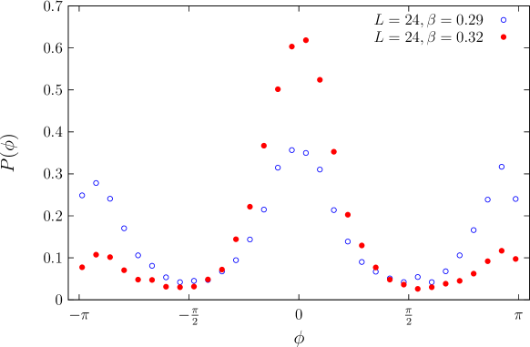
Figure 2: Distribution of spin phases in a single typical configuration of the spin system in the disordered (circles) and in the ordered (full points) phases. Here $h=1.0$ and $L=24$.

Since our toy model is quenched, in the ordered phase of the spin model we have to select the appropriate vacuum by hand. The appropriate vacuum is of course that in which the phase of the magnetisation $m=N_{c}^{-1}L^{-3}\sum_{\vec{x},a}s^{a}_{\vec{x}}=|m|e^{i\varphi_{m}}$ is zero, corresponding to the trivial Polyakov loop sector selected by fermions in QCD. This is done in practice only at the level of the random Hamiltonian, by “rotating” the spins, i.e., aligning their phase to zero, when the spin model is in a different vacuum. In the case $N_{c}=2$ considered in this paper this is easy to implement. For typical configurations in the ordered phase, the (complex) magnetisation is usually close to being real, i.e., $e^{i\varphi_{m}}\simeq\pm 1$. When $\cos\varphi_{m}<0$, we “rotate” all the spins by replacing $s_{\vec{x}}\to-s_{\vec{x}}$. In terms of the phases $\phi_{\vec{x}}\in[-\pi,\pi)$, this is implemented through

$$\phi_{\vec{x}}\to\phi_{\vec{x}}-\pi\,{\rm sign}(\phi_{\vec{x}})\,,\qquad{\rm sign}(0)\equiv 1\,.$$ (34)

The spectral density $\rho(\lambda)$ of the random Hamiltonian in the two phases is shown in Fig. 3: while in the disordered phase ($\beta<\beta_{c}$) there is an accumulation of eigenvalues near the origin, so that (presumably) $L^{-3}\rho(0)\neq 0$ in the thermodynamic limit, in the ordered phase ($\beta>\beta_{c}$) this region is depleted, and $\rho(0)=0$. The dependence on $\beta$ is rather mild in the disordered phase, while the spectral density gets rapidly suppressed as $\beta$ grows in the ordered phase. The expected connection between magnetisation in the spin system and “chiral” transition in the spectrum of the random Hamiltonian indeed shows up.

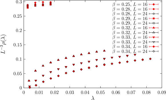
Figure 3: Spectral density of the toy Hamiltonian for several values of $\beta$ and different volumes. Here $h=1.0$ and $\hat{\beta}=5.0$.

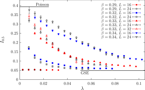
Figure 4: Spectral statistics $I_{0.5}$ along the spectrum for several values of $\beta$ and different volumes. Here $h=1.0$ and $\hat{\beta}=5.0$.

In order to understand the nature of the lowest eigenmodes in the two phases, it is convenient to study the statistical properties of the corresponding eigenvalues. In fact, localised modes are expected to fluctuate independently, so that the corresponding eigenvalues should obey Poisson statistics. Delocalised modes, on the other hand, mix strongly under fluctuations and are expected to obey the appropriate Wigner–Dyson statistics, which in the case at hand is the one corresponding to the Gaussian Symplectic Ensemble (GSE). A convenient observable to distinguish the two cases is the spectral statistics $I_{0.5}$ SSSLS ; HS ,

$$I_{0.5}\equiv\int_{0}^{0.5}ds\,P_{\rm ULSD}(s)\,,$$ (35)

where $P_{\rm ULSD}(s)$ is the probability distribution of the unfolded level spacings $s_{j}=\frac{\lambda_{j+1}-\lambda_{j}}{\langle\lambda_{j+1}-\lambda_{j}\rangle}$, where $\langle\lambda_{j+1}-\lambda_{j}\rangle$ is the average level spacing in the spectral region corresponding to the given level. Unfolding is a mapping of the eigenvalues that makes the spectral density equal to 1 throughout the spectrum. In practice, we have ordered the eigenvalues obtained in all the explored spin configurations and replaced them by their rank divided by the number of configurations. The $P_{\rm ULSD}(s)$ is known both in the case of Poisson statistics, where it is the exponential distribution $P_{\rm P}(s)=\exp(-s)$, and in the case of the GSE, where it is very precisely approximated by the symplectic Wigner surmise $P_{\rm GSE}$ Mehta ,

$$P_{\rm GSE}(s)=\left(\frac{64}{9\pi}\right)^{3}s^{4}\exp\left(-\frac{64}{9\pi}s^{2}\right)\,.$$ (36)

The quantity $I_{0.5}$ is sensitive to the behaviour of $P_{\rm ULSD}(s)$ near $s=0$, and so it is very different for Poisson (where $P_{\rm P}\sim 1$ near $s=0$) and GSE ($P_{\rm GSE}\sim s^{4}$) statistics. Indeed, $I_{0.5}^{\rm GSE}\simeq 0.0487$ for the GSE, while for the Poisson ensemble $I_{0.5}^{\rm P}\simeq 0.393$. The choice of the upper limit of integration in Eq. (35) is made in order to maximise the difference between these two values, as $P_{\rm P}$ and $P_{\rm GSE}$ cross near $s=0.5$. In Fig. 4 we show the behaviour of $I_{0.5}$ as one moves along the spectrum, i.e., computing $I_{0.5}$ locally, using only eigenvalues in disjoint bins of fixed width, and assigning the result to the average of the eigenvalues in that bin. While in the disordered phase one finds Wigner–Dyson statistics throughout the whole spectrum, in the ordered phase the lowest modes have near-Poisson statistics, and become more independent as the volume is increased. Above a $\beta$-dependent point $\lambda_{c}$ in the spectrum, the modes have near-Wigner–Dyson behaviour, and more and more so when the volume is increased. This hints at a localisation/delocalisation transition in the spectrum taking place in the thermodynamic limit. As the system is made more ordered, $\lambda_{c}$ increases, which is in agreement with our expectations: qualitatively, $\lambda_{c}$ should behave like the spatial average of the lowest effective Matsubara frequency GKP , which indeed grows as the ordering of the system is increased. Our toy model is therefore able to reproduce localisation of the low modes in the ordered phase, and the qualitative dependence of the “mobility edge” $\lambda_{c}$ on the ordering of the system.

The results discussed above show that our toy model successfully reproduces the important features of QCD for what concerns localisation and “chiral symmetry” breaking/restoration, i.e., the accumulation or not of eigenvalues near the origin. This indicates that we have indeed kept all the important aspects of the Dirac operator and of the gauge dynamics in our model, which can thus be used to gain some reliable qualitative insight into the properties of the Dirac eigenvalues and eigenmodes. Therefore, although the following discussion deals explicitly with the toy model, it can be directly translated to the physically relevant case of QCD by replacing “spins” with Polyakov line phases.

4.1 Variations on the toy model

We want now to test how the features of the toy model that we borrowed from QCD affect the “chiral” transition, i.e., the drop in the spectral density near the origin, and localisation of the lowest modes. To this end, we study some ad hoc modifications of the toy model.

The “chiral” transition and localisation of the lowest modes are clearly connected in our toy model, as they are evidently tied to the magnetisation of the spin system. The magnetisation affects our toy model Hamiltonian in two ways: it creates a “sea” of ordered spins, where “islands” of fluctuations provide an “energetically” convenient place for an eigenmode to localise BKS ; GKP ; and it locally correlates the gauge links on different time slices, thus leading to the approximate local decoupling of different temporal-momentum components of the eigenfunctions. It is an interesting question how important each of these two effects is for “chiral symmetry” breaking and localisation.

As a matter of fact, the appearance of “islands” alone is not enough to produce either “chiral symmetry” restoration or localisation. In Fig. 5 we show the spectral density and the spectral statistic $I_{0.5}$ obtained in the ordered phase at $\beta=0.32$ when setting $\hat{\beta}=0$, i.e., imposing no correlation between the time slices. In this case, despite the presence of “islands” in the spin configurations, the spectral density at the origin remains finite, and the low-lying eigenmodes do not localise. This means that to restore “chiral symmetry” one needs that the mixing of different temporal-momentum components of the quark wave functions be suppressed to some extent. Only then can the “islands” effectively act as localising centers for the low modes, since, loosely speaking, the lowered spectral density would make it difficult to mix for modes localised in different regions.

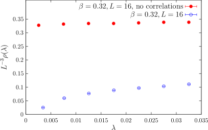
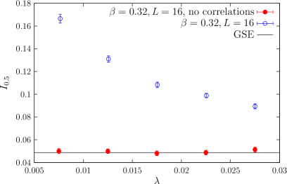
Figure 5: Comparison between the toy model in the ordered phase with (circles, $\hat{\beta}=5.0$) and without (full points, $\hat{\beta}=0.0$) correlation between gauge links on different time slices: spectral density (left panel) and $I_{0.5}$ (right panel). Here $L=16$ and $\beta=0.32$.

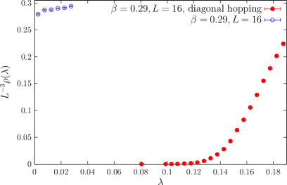
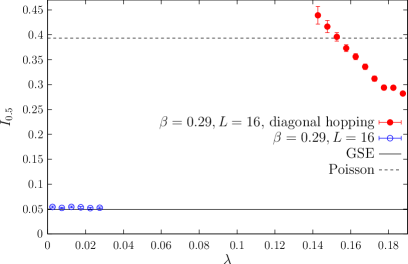
Figure 6: Comparison between the toy model in the disordered phase with (circles) and without (full points) off-diagonal hopping terms in temporal-momentum space: spectral density (left panel) and $I_{0.5}$ (right panel). Here $L=16$ and $\beta=0.29$.

On the other hand, in the disordered phase the absence of “islands” is not sufficient to ensure “chiral symmetry” breaking and prevent localisation of the lowest modes. An essential ingredient for the accumulation of eigenvalues around the origin is the fact that the hopping term has typically sufficiently large off-diagonal components in temporal-momentum space. In Fig. 6 we show the spectral density obtained in the disordered phase at $\beta=0.29$ when setting the off-diagonal part of the hopping term to zero. The Hamiltonian in this case is block-diagonal in temporal-momentum space, with blocks ${\cal H}^{[\pm]}$ of the form

$${\cal H}^{[\pm]}(\vec{x},\vec{y})=[\pm]\eta_{4}(x)c(\vec{x})\,\delta_{\vec{x}\vec{y}}+\sum_{j=1}^{3}\frac{\eta_{j}(\vec{x})}{2i}\left(v_{+j}^{(+)}(\vec{x})\,\delta_{\vec{x}+\hat{\jmath},\vec{y}}-v_{-j}^{(+)}(\vec{x})\,\delta_{\vec{x}-\hat{\jmath},\vec{y}}\right)\,,$$ (37)

where $[c(\vec{x})]_{ab}=\cos{\textstyle\frac{\phi_{\vec{x}}}{2}}\,\delta_{ab}$, and ${v}_{\pm j}^{(+)}$ have been defined in Eq. (31). Apart from the presence of colour, and of disorder in the hopping terms, this is precisely the Hamiltonian considered in Ref. GKP . In this case the spectrum displays a sharp gap near the origin. In Fig. 6 we also show how the spectral statistic $I_{0.5}$ changes along the spectrum. Our results show that the lowest-lying modes are localised, while higher up in the spectrum they delocalise, as signalled by the decrease of $I_{0.5}$. The reason why $I_{0.5}$ does not tend to the GSE value in the bulk, but remains clearly above it, can be ascribed to the fact that the spectra of ${\cal H}^{[\pm]}$ are separately symmetric on average with respect to the origin. The proof of this property can be easily obtained extending the one reported in Ref. GKP to the case of nontrivial hopping terms and in the presence of colour. Combining the two spectra together to obtain that of ${\cal H}^{\rm toy}$, one expects that the latter will have an approximate double degeneracy (on top of the Kramers degeneracy) of the eigenvalues. This naturally leads to an enhancement of the ULSD near the origin (levels like to lie closer than on average) with respect to the Wigner–Dyson distribution, and therefore to an enhancement of $I_{0.5}$.

The results above show that the mixing of different temporal momentum components is a necessary condition to have chiral symmetry breaking in the disordered phase, and that its (local) attenuation is a necessary condition to have restoration in the ordered phase. This entails that the “minimal” model studied here is indeed minimal, if one wants to reproduce qualitatively the features of the Dirac spectrum and of the corresponding eigenmodes. It is thus not possible to neglect entirely the temporal direction, as in Ref. GKP , if one wants to correctly describe the disordered phase. Furthermore, in the present setting one cannot neglect the correlation of spatial links across time slices if one wants restoration of chiral symmetry and localisation of the low modes in the ordered phase. However, one cannot certainly conclude that those described above are also sufficient conditions, especially because of the extreme nature of the two modifications of the toy model that we have studied. In a realistic situation, correlations across time slices are always present to some extent, but never perfect, so that mixing of the temporal components of the quark wave functions is never completely free or strictly forbidden. One thus expects some other effect to compete against mixing, with the fate of “chiral symmetry” and localisation being decided by the strongest of the two effects. The obvious candidate is the nature of the diagonal disorder, i.e., of the distribution of the unperturbed eigenvalues: for a low density of small unperturbed modes it should be more difficult to accumulate eigenvalues around the origin, and conversely for a high density of such unperturbed modes a weak mixing of temporal momentum components could be sufficient.

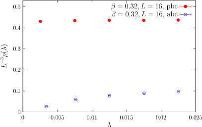
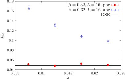
Figure 7: Comparison between the toy models obtained in correspondence to periodic (“pbc”, full points), or antiperiodic (“abc”, circles) boundary conditions for the fermions, in the ordered phase of the spin model: spectral density (left panel) and $I_{0.5}$ (right panel). Here $L=16$ and $\beta=0.32$.

The latter case is naturally illustrated by changing the boundary conditions for the fermions in the temporal direction from antiperiodic to periodic. The derivation of the Dirac-Anderson Hamiltonian proceeds exactly in the same way, and leads to the same results, Eqs. (11) and (12), up to replacing the “fermionic” Matsubara frequencies $\omega_{ak}(\vec{x})$ with the “bosonic” frequencies $\omega^{\rm PBC}_{ak}(\vec{x})$,

$$\omega^{\rm PBC}_{ak}(\vec{x})={\textstyle\frac{1}{N_{T}}}(\phi_{a}(\vec{x})+2\pi k)\,,\qquad k=0,1,\ldots,N_{T}-1\,.$$ (38)

The construction of the toy model is also unchanged, up to a similar replacement in the diagonal terms, Eq. (22). In the minimal setting $N_{T}=N_{c}=2$, this amounts to replace $\cos\frac{\phi_{\vec{x}}}{2}\to\sin\frac{\phi_{\vec{x}}}{2}$. In the ordered phase the distribution of unperturbed eigenvalues is now peaked around zero, while the correlations between spatial links and thus the strength of the mixing of the temporal momentum components are unchanged. Numerical results for this model are shown in Fig. 7: “chiral symmetry” is broken and localisation is absent. Notice that this is precisely what one expects, if the toy model is to correctly reproduce the features of QCD CC ; Step , which further supports the viability of our model to study the qualitative behaviour of the Dirac spectrum.

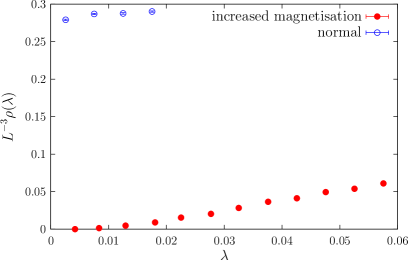
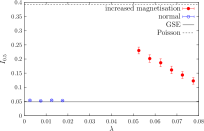
Figure 8: Comparison between the toy model in the disordered phase and the artificial model obtained by increasing the unperturbed eigenvalues via the mapping $f_{\tau}$ described in the text: spectral density (left panel) and $I_{0.5}$ (right panel). Here $L=16$, $\beta=0.29$ and $\tau=0.2$.

To illustrate the former case we have employed a more artificial construction, increasing “by hand” the ordering of the unperturbed eigenvalues while keeping unchanged the hopping terms. This has been achieved by mapping the absolute value of the unperturbed eigenvalues, $z_{\vec{x}}=\cos\frac{\phi_{\vec{x}}}{2}$, to $f_{\tau}(z_{\vec{x}})=\frac{2z_{\vec{x}}^{\tau}}{1+z_{\vec{x}}^{2\tau}}$ with $0<\tau<1$. As we show in Fig. 8, in this way one can deplete the spectral region around zero: the strength of the temporal-momentum-component mixing is not sufficient to compensate for the lowered density of small unperturbed modes.

4.2 Discussion

Summarising our findings, the fate of “chiral symmetry” and of localisation depends on the competition between ordering of the unperturbed modes and mixing of temporal momentum components of the wave functions. In the disordered phase, when there is no ordering of the unperturbed modes and a sizeable amount of small such modes is present, there is actually no competition and one expects chiral symmetry to be broken. In the ordered phase, the reduction of mixing can be compensated by changing the boundary conditions, so increasing the amount of small unperturbed modes. Although we have checked here only the case of periodic boundary conditions, one can in principle change the effective boundary conditions in a continuous manner by introducing an imaginary chemical potential, $\mu$: periodic boundary conditions thus correspond to $|\mu N_{T}|=\pi$, and for $|\mu N_{T}|$ sufficiently close to $\pi$ we still expect to find a finite spectral density at the origin. Sticking to $N_{c}=2$ and feeding this back into the partition function by including the fermionic determinant, in the ordered/deconfined phase one is lead to expect that if at $\mu=0$ the trivial center sector is selected, at $|\mu N_{T}|=\pi$ the system is again in the ordered/deconfined phase but in the other center sector. For sufficiently high temperature one thus expects to find a transition from one vacuum to the other when moving along the $\mu$ direction in the phase diagram, which then repeats due to periodicity in $\mu$: these are nothing but the Roberge-Weiss transitions RW .

Our results shed some more light on the “sea/islands” mechanism in QCD, and on its ineffectiveness at low temperature. As we have said above, in the disordered phase the hopping term has typically sizeable off-diagonal entries, which can effectively mix different temporal-momentum components of the quark wave function. This is due to the presence of extended spatial regions where the local correlations across time slices are sufficiently weak, because of the lack of order in the underlying spin system. As we saw above, this is necessary for the accumulation of small eigenvalues, and one can think of mixing as somehow “pushing” the eigenvalues towards zero. On top of that, the lack of order also provides a sizeable density of small unperturbed modes, which also favours such an accumulation. The combination of these two effects thus leads naturally to a finite spectral density near the origin, and to delocalisation of the low modes. The ineffectiveness of the “sea/islands” mechanism at low temperatures is thus due to the fact that in that case there simply are no “islands”. In contrast to this, in the ordered phase the regions where mixing is effective are localised on the “islands” where the spins fluctuate away from the ordered value. In the “sea” of ordered spins the unperturbed eigenvalues are large (i.e., close to 1) and the mixing of different temporal-momentum components is suppressed, so that the “push” towards the origin is weaker, and the “sea” does not contribute to the accumulation of eigenvalues around the origin. Low modes thus originate from the “islands”, and this naturally leads to their localisation and to a small spectral density near zero.

There is another important aspect involved in chiral symmetry breaking or restoration. For any finite volume, the spectral density decreases to zero within a sufficiently small distance from the origin. What actually determines the fate of chiral symmetry is how this distance scales with the volume of the system. In the disordered phase, the small eigenvalues originate from small unperturbed modes that occupy a finite fraction of the volume. The “push” caused by mixing of the temporal-momentum components is thus expected to scale with the system size, eventually leading to a finite spectral density at the origin in the thermodynamic limit. In the ordered phase, the small eigenvalues originate from small unperturbed modes localised on the “islands”, and the strength of the “push” coming from mixing is expected to correspond to the size of the “islands”, which does not scale with the system size, so that the spectral density at the origin remains zero also in the thermodynamic limit.

Before concluding this Section, we want to list a few issues which remain open. We have not checked whether the “chiral” transition in our model is a genuine phase transition in the thermodynamic limit, and if so whether it takes place exactly together with the transition in the spin system. We also have not checked the dependence on the strength $h$ of the $U(1)^{N_{c}-1}$-symmetry-breaking term in the Hamiltonian of the spin system. As this would change the depth of the symmetry-breaking potential, it can in principle affect the nature of the transition in the spin system, and so in turn that of the “chiral” transition. Moreover, we have not investigated in details how our results change when changing the parameter $\hat{\beta}$, which affects the strength of the correlation between time slices. Since the amount of small unperturbed modes is unaffected by such a change, it is reasonable to expect that a larger $\hat{\beta}$, increasing the correlations and thus reducing the mixing between wave function components corresponding to different temporal momenta in the “sea” region, will make the change in the spectral density when going over to the ordered phase even more dramatic. Similarly, a smaller $\hat{\beta}$ is expected to make this change less dramatic, and for small enough $\hat{\beta}$ we expect that “chiral symmetry” is broken also in the ordered phase of the spin model, by continuity with the $\hat{\beta}=0$ result discussed above. However, it is not clear if the value of $\hat{\beta}$ can affect the nature of the “chiral” transition, i.e., whether it is a true phase transition or a crossover, and the value of $\beta$ at which it takes place. Nevertheless, we think that the connection between correlation of spatial links across time slices and fate of “chiral symmetry” is strongly supported by our findings.

5 Conclusions

In this paper we have studied the problems of chiral symmetry breaking and localisation in finite-temperature QCD by looking at the lattice Dirac operator as a random Hamiltonian. We have explicitly recast the staggered Dirac operator at finite temperature in the form of a non-conventional 3D Anderson Hamiltonian (“Dirac-Anderson Hamiltonian”), which describes fermions carrying colour and an extra internal degree of freedom, corresponding to the lattice temporal momenta. The on-site noise is provided by the phases of the Polyakov lines, and their ordering, or the lack thereof, reflects in the distribution of the diagonal entries of the Hamiltonian. The Polyakov lines affect the hopping terms as well. Indeed, in the deconfined phase they induce strong correlations among spatial links on different time slices, in the region where they are aligned with the identity. This in turn weakens the coupling among the components of the wave function corresponding to different lattice temporal momenta on neighbouring sites. In the confined phase, on the other hand, such strong correlations are absent due to the absence of order, and these wave function components can mix effectively. We think that this difference in the hopping terms is essential to explain the accumulation or not of eigenvalues near the origin, and ultimately for the spontaneous breaking or not of chiral symmetry. The other important difference between the two phases concerns the density and spatial distribution of small unperturbed eigenvalues, i.e., of small diagonal entries, which is also caused by the different ordering properties of the Polyakov lines. We think that these two properties of the small unperturbed eigenvalues are also essential in explaining the fate of chiral symmetry. Furthermore, the fact that the small unperturbed eigenvalues appear in localised spatial regions at high temperature leads to the localisation of the low Dirac eigenmodes. This suggests that the confinement/deconfinement transition triggers both the chiral transition and the localisation of the low modes.

To test this picture we have constructed a toy model, made up of a spin system with dynamics similar to that of the Polyakov line phases in QCD; of unitary matrices obeying dynamics analogous to the dynamics of spatial gauge links in the background of fixed Polyakov lines; and of a random Hamiltonian with the same structure as the Dirac-Anderson Hamiltonian discussed above, with on-site noise provided by the spins. This toy model is designed to keep precisely the features of QCD which we believe to be relevant to the phenomena of chiral symmetry breaking (which means here a nonzero spectral density at the origin) and localisation. A numerical study of the toy model, in the simplest case of two colours and two time slices, shows that it indeed displays both these phenomena, with the same qualitative dependence on the ordering of the noise source (spins/Polyakov lines) as in QCD. When the noise source is disordered there is chiral symmetry breaking but no localisation; when the noise source is ordered chiral symmetry is restored and low modes are localised, up to a point in the spectrum (“mobility edge”) which is pushed towards larger values as the ordering is increased. If, on the other hand, one artificially removes the correlation between the time slices in the ordered phase, then chiral symmetry remains broken and there is no localisation. Moreover, if the mixing between components corresponding to different time-momenta is artificially removed in the disordered phase, then chiral symmetry is restored and the lowest modes localise. These findings support, and actually suggested, that the correlation among time slices and the related mixing of temporal-momentum components of the quark wave functions play an essential role in the chiral transition and in the appearance of localised modes. The importance of the role played by the small unperturbed eigenvalues is made evident by the results obtained when one imposes on the fermions periodic rather than antiperiodic boundary conditions in the temporal direction. In this case the properly modified toy model again reproduces qualitatively the QCD results, with accumulation of eigenvalues around the origin and no localisation also in the ordered phase. Since the hopping terms are exactly the same as with antiperiodic boundary conditions, one is led to conclude that even with weak mixing between temporal-momentum components one can achieve chiral symmetry breaking, if the density of small unperturbed modes is large enough. Conversely, by artificially increasing the unperturbed modes without touching the hopping terms, one can restore chiral symmetry in the disordered phase and make the low Dirac modes localised, which indicates that strong mixing may be insufficient to accumulate eigenvalues around zero if the density of small unperturbed modes is too low.

The results obtained in the toy model support our expectation that in QCD the fate of chiral symmetry and of localisation are closely related, and furthermore that both depend on the amount of small unperturbed modes and on the mixing of temporal-momentum components of the quark wave functions, therefore ultimately on the distribution of the phases of the Polyakov lines.

The picture discussed here makes no direct reference to topology. As is well known, in the “topological” explanation of chiral symmetry breaking the finite density of near-zero modes originates from fermionic zero modes supported by topological objects, which broaden into a band due to mixing. The localised nature of these modes would also explain localisation at high temperature. In the Dirac-Anderson picture, the “unperturbed” small modes have a different origin, being the eigenmodes of the temporal part of the Dirac operator, and moreover the way they mix (i.e., the nature of the hopping terms) is also expected to play an important role in the accumulation of near-zero modes and in their localisation properties. It is of course well possible that the two pictures are just complementary point of views on the same phenomenon, corresponding to a different way to separate the full Dirac operator into a “free” and an “interaction” part. In light of the close connection between the chiral transition and localisation, and of the central role played by the Polyakov lines in both phenomena, we expect that if this is the case, then the topological objects relevant to chiral symmetry breaking at low temperature, and to localisation at high temperature, would also be relevant to the deconfinement transition. Indeed, there are numerical results pointing to a close relation between localisation and certain topological objects which are expected to play a role in the deconfinement transition Cossu:2016scb . This issue certainly deserves more work. Attention should also be paid to the possible relation between localisation and chiral symmetry restoration, on one side, and “non-topological” approaches to confinement like, e.g., “fluxons” Mandelstam:1974pi ; 'tHooft:1977hy .

It would be interesting to further investigate in our toy model the behaviour of the spectrum in the vicinity of the phase transition in the spin model. This would clarify if the “chiral transition” seen there is actually a genuine phase transition, and how close it takes place to the magnetic transition. This could provide useful insight in the critical properties at the chiral transition of the “parent” physical system, namely, QCD. Furthermore, one could check how the transition is affected by the strength of the coupling between spatial links on different time slices, and by the depth of the minimum of the spin potential, which are parameters of the model besides the temperature of the spin system.

An obvious extension of this work would be to check the ideas presented above directly with QCD gauge configurations, using the Dirac-Anderson form of the Dirac operator to tweak the hopping terms independently of the underlying Polyakov-line dynamics. While the toy model studied here is quenched, with no backreaction of the quark eigenvalues in the partition function, the main ideas are expected to apply in the presence of dynamical fermions as well.

It would be interesting to try to apply the ideas discussed in this paper in the case when a constant (Abelian) magnetic field is turned on. This could shed some light on the issue of (inverse) magnetic catalysis of the quark condensate imc1 ; imc2 . Another interesting application would be to the case of nonzero imaginary chemical potential, already very briefly discussed here.

Another interesting testing ground for the proposed mechanism is the explanation of the separate occurrence of the deconfinement and chiral transitions in $SU(3)$ gauge theory with adjoint fermions adjoint . Since the derivation of the Dirac-Anderson Hamiltonian did not use in an essential way that we were considering fundamental fermions, the same form holds for adjoint fermions, replacing gauge links with their adjoint counterpart, and the $N_{c}$ phases of the fundamental Polyakov line with the $N_{c}^{2}-1$ phases of the adjoint Polyakov line.

In conclusion, we believe that the “Dirac-Anderson” approach of the present paper to the study of the quark eigenvalues and eigenfunctions can lead to a better understanding of the phase structure of QCD and related theories.

Appendix A Properties of the hopping term

In this Appendix we describe in some detail the properties of the QCD Dirac-Anderson “Hamiltonian”, and in particular of its hopping terms, ${\cal V}_{\pm j}$. First of all, notice that

$$\left[{\cal V}^{\dagger}_{\pm j}(\vec{x},\vec{y})\right]_{ak,bl} =\left[{\cal V}^{*}_{\pm j}(\vec{y},\vec{x})\right]_{bl,ak}=\delta_{\vec{x}\mp\hat{\jmath},\vec{y}}\frac{1}{N_{T}}\sum_{t=0}^{N_{T}-1}e^{-i\frac{2\pi t}{N_{T}}(k-l)}\left[\tilde{U}^{*}_{\pm j}(t,\vec{y})\right]_{ba}$$ (39)

$$=\delta_{\vec{x}\mp\hat{\jmath},\vec{y}}\frac{1}{N_{T}}\sum_{t=0}^{N_{T}-1}e^{i\frac{2\pi t}{N_{T}}(l-k)}\left[\tilde{U}^{\dagger}_{\pm j}(t,\vec{x}\mp\hat{\jmath})\right]_{ab}$$

$$=\delta_{\vec{x}\mp\hat{\jmath},\vec{y}}\frac{1}{N_{T}}\sum_{t=0}^{N_{T}-1}e^{i\frac{2\pi t}{N_{T}}(l-k)}\left[\tilde{U}_{\mp j}(t,\vec{x})\right]_{ab}=\left[{\cal V}_{\mp j}(\vec{x},\vec{y})\right]_{ak,bl}\,,$$

as it should. From now on we will often omit matrix indices, so we remind the reader that $\tilde{U}_{\pm j}(t,\vec{x})$ has only colour indices, while $D(\vec{x})$ and $V_{\pm j}(\vec{x})$ have both colour and temporal-momentum indices. The identity in these spaces will be denoted by $\mathbf{1}_{\rm c}$ and $\mathbf{1}_{\rm tm}$, respectively. Since $\tilde{U}_{\pm j}(t,\vec{x})$ are unitary matrices,

$$\tilde{U}_{\pm j}(t,\vec{x})[\tilde{U}_{\pm j}(t,\vec{x})]^{\dagger}=\mathbf{1}_{\rm c}\,,$$ (40)

$$\det\tilde{U}_{\pm j}(t,\vec{x})=e^{i\frac{2\pi t}{N_{T}}[q(\vec{x}\pm\hat{\jmath})-q(\vec{x})]}\,,\quad 2\pi q(\vec{x})=\sum_{a=1}^{N_{c}}\phi_{a}(\vec{x})\,,\quad q(\vec{x})\in\mathbb{Z}\,,$$

and since $V_{\pm j}(\vec{x})$ is the Fourier transform with respect to time of the unitary matrix $\bar{U}_{\pm j}(\vec{x})$,

$$V_{\pm j}(\vec{x})=F\bar{U}_{\pm j}(\vec{x})F^{\dagger}\,,$$ (41)

where

$$\left[\bar{U}_{\pm j}(\vec{x})\right]_{at,bt^{\prime}}=\delta_{tt^{\prime}}\left[\tilde{U}_{\pm j}(t,\vec{x})\right]_{ab}\,,\qquad F_{kt}=\frac{1}{\sqrt{N_{T}}}\,e^{-i\frac{2\pi t}{N_{T}}kt}\,,$$ (42)

with $FF^{\dagger}=\mathbf{1}_{\rm tm}$, we conclude that $V_{\pm j}(\vec{x})$ is also unitary in colour and temporal-momentum space,

$$V_{\pm j}(\vec{x})V_{\pm j}(\vec{x})^{\dagger}=\mathbf{1}_{\rm c}\mathbf{1}_{\rm tm}\,.$$ (43)

Moreover, since (recall that $N_{T}$ is even)

$$\det V_{\pm j}(\vec{x})=\prod_{t=0}^{N_{T}-1}e^{i\frac{2\pi t}{N_{T}}[q(\vec{x}\pm\hat{\jmath})-q(\vec{x})]}=e^{i\pi[q(\vec{x}\pm\hat{\jmath})-q(\vec{x})](N_{T}-1)}=e^{-i\pi[q(\vec{x}\pm\hat{\jmath})-q(\vec{x})]}=\pm 1\,,$$ (44)

we have that $V_{\pm j}(\vec{x})$ is also unimodular up to a sign. If we choose one and the same convention for the phases of the local Polyakov lines, i.e., we fix $q(\vec{x})=q~{}\forall\vec{x}$, then $V_{\pm j}(\vec{x})\in SU(N_{c}\times N_{T}),~{}\forall\vec{x},j$. However, one can choose different phase conventions at different spatial points, and still obtain the same physical results. We will return below to this issue. We observe also the following cyclicity property of $V_{\pm j}(\vec{x})$,

$$\left[V_{\pm j}(\vec{x})\right]_{a(k+n)_{N_{T}},b(l+n)_{N_{T}}}=\left[V_{\pm j}(\vec{x})\right]_{ak,bl}\,,\,\,\forall n\in\mathbb{Z}\,.$$ (45)

One can easily verify that this property is preserved under multiplications, so $V_{\pm j}(\vec{x})$ belong to the “$(N_{T}\times N_{T})$-block cyclic” subgroup of $SU(N_{c}\times N_{T})$.

Let us now return to the issue of the choice of phase conventions. All $\phi_{a}(\vec{x})$ are defined modulo $2\pi$, so after a redefinition $\phi_{a}(\vec{x})\to\phi_{a}(\vec{x})+2\pi q_{a}(\vec{x})$ with $q_{a}(\vec{x})\in\mathbb{Z}$ one should obtain equivalent results. We will denote quantities after the redefinition with the superscript $\{q\}$. We have for the effective Matsubara frequencies

$$\exp[i\omega_{ak}^{\{q\}}(\vec{x})]=\exp\left[i\textstyle{\frac{1}{N_{T}}}(\pi+\phi_{a}(\vec{x})+2\pi q_{a}(\vec{x})+2\pi k)\right]=\exp[i\omega_{a(k+q_{a}(\vec{x}))_{N_{T}}}(\vec{x})]\,,$$ (46)

so that the temporal-momentum indices of $D(\vec{x})$ and $V_{\pm j}(\vec{x})$ undergo a colour-dependent cyclic permutation $k\to k+q_{a}(\vec{x})\mod N_{T}$. This can be written formally using the permutation matrices $\Pi^{(n)}$,

$$\Pi^{(n)}_{kk^{\prime}}=\delta_{(k+n)_{N_{T}}k^{\prime}}\,,\quad\Pi^{(n)}[\Pi^{(n)}]^{\dagger}=\Pi^{(n)}[\Pi^{(n)}]^{T}=\mathbf{1}_{\rm tm}\,,$$ (47)

by setting

$$\left[Z^{\{q\}}(\vec{x})\right]_{ak,bl}=\Pi^{(q_{a}(\vec{x}))}_{kl}\delta_{ab}\,.$$ (48)

We then have

$$D^{\{q\}}(\vec{x})={Z}^{\{q\}}(\vec{x})D(\vec{x}){Z}^{\{q\}}(\vec{x})^{\dagger}\,,\qquad V^{\{q\}}_{\pm j}(\vec{x})={Z}^{\{q\}}(\vec{x})V_{\pm j}(\vec{x}){Z}^{\{q\}}(\vec{x}\pm\hat{\jmath})^{\dagger}\,.$$ (49)

Notice that $V_{\pm j}(x)$ is left invariant if $q_{a}(\vec{x})=q_{b}(\vec{x}\pm\hat{\jmath})~{}\forall a,b$, as a consequence of its cyclicity property. Finally, defining

$$\left[{\cal Z}^{\{q\}}(\vec{x},\vec{y})\right]_{ak,bl}=[Z^{\{q\}}(\vec{x})]_{kl}\,\delta_{ab}\,\delta_{\vec{x}\vec{y}}\,,\qquad{\cal Z}^{\{q\}}{\cal Z}^{\{q\}}{}^{\dagger}=\mathbf{1}_{\rm c}\mathbf{1}_{\rm tm}\mathbf{1}_{\rm sp}\,,$$ (50)

with $\mathbf{1}_{\rm sp}$ the identity in spatial-coordinate space, we can write in compact form

$${\cal H}^{\{q\}}={\cal Z}^{\{q\}}{\cal H}{\cal Z}^{\{q\}\,{\dagger}}\,,$$ (51)

which amounts to say that a redefinition of the phases corresponds to a unitary transformation of the Hamiltonian, which therefore leaves the spectrum unchanged.

It is interesting to notice that if we make the unitary transformation Eq. (51) setting $q_{a}(\vec{x})=\frac{N_{T}}{2}~{}\forall\vec{x},a$, then, denoting $\tilde{\cal Z}={\cal Z}^{\{q_{a}(\vec{x})=\frac{N_{T}}{2}\}}$, we find [see Eq. (8)]

$$\tilde{\cal Z}{\cal H}\tilde{\cal Z}^{\dagger}=-{\cal D}(\vec{x},\vec{y})+\sum_{j=1}^{3}\frac{\eta_{j}(\vec{x})}{2i}\left\{{\cal V}_{+j}(\vec{x},\vec{y})-{\cal V}_{-j}(\vec{x},\vec{y})\right\}=-\eta_{4}{\cal H}\eta_{4}\,,$$ (52)

where $(\eta_{4}{\cal H}\eta_{4})(\vec{x},\vec{y})=\eta_{4}(\vec{x}){\cal H}(\vec{x},\vec{y})\eta_{4}(\vec{y})$. We conclude that ${\cal Q}\equiv\eta_{4}\tilde{\cal Z}$ satisfies $\{{\cal Q},{\cal H}\}=0$, which implies that the spectrum is symmetric with respect to $\lambda=0$, as it should be for staggered fermions.

One final remark is in order concerning the case of gauge group $SU(2)$. In this case one has $\phi_{1}=-\phi_{2}\equiv\phi$. It is known that in this case the Dirac operator has an antiunitary symmetry ${\cal T}$ with ${\cal T}^{2}=-1$ VWrev . In the new basis, taking the complex conjugate of ${\cal H}$ has the effect of (i) exchanging the indices $k,l$ in temporal-momentum space, (ii) changing the sign of the phases $\phi$ appearing in $\tilde{U}$ [Eq. (12)] and taking the complex conjugate of the $SU(2)$ matrices ${U}^{\rm(td)}_{\pm j}$, and (iii) changing the overall sign of the hopping terms. Point (ii) can be “undone” by taking the matrix conjugate with respect to $\sigma_{2}$ in colour space (this remains true also in the presence of nontrivial phases $\phi$, as can be directly checked); this also leads to the diagonal element $k$ being switched with the element $\frac{N_{T}}{2}-1-k$. Indeed, matrix conjugation by $\sigma_{2}$ exchanges the diagonal terms corresponding to $\phi$ and $-\phi$, and this is equivalent to switching temporal-momentum components, since

$$\sin{\textstyle\frac{\pi-\phi+2\pi k}{N_{T}}}=\sin{\textstyle\frac{\pi+\phi+2\pi\left({\textstyle\frac{N_{T}}{2}}-1-k\right)}{N_{T}}}\,.$$ (53)

This corresponds to a permutation $\Pi$ of the temporal-momentum components defined so that $k\to\frac{N_{T}}{2}-1-k\mod N_{T}$ (notice $\Pi^{2}=1$). Since the hopping term depends on $k,l$ only through $k-l$, one has $l-k=\left(\frac{N_{T}}{2}-1-k\right)-\left(\frac{N_{T}}{2}-1-l\right)$, and so by applying $\Pi$ we undo both point (i) and the above-mentioned effect on the diagonal term. Finally, taking the matrix conjugate with respect to $\eta_{4}$ in spatial-coordinate space we undo point (iii). All in all, ${\cal T}=\eta_{4}\Pi\sigma_{2}K$, with $K$ the complex conjugation, is an antiunitary symmetry of the Hamiltonian with ${\cal T}^{2}=-\sigma_{2}^{2}=-1$.

References

- (1) T. Banks and A. Casher, Nucl. Phys. B 169 (1980) 103.
- (2) J. J. M. Verbaarschot and T. Wettig, Ann. Rev. Nucl. Part. Sci. 50 (2000) 343 [hep-ph/0003017].
- (3) P. de Forcrand, AIP Conf. Proc. 892 (2007) 29 [hep-lat/0611034].
- (4) A. M. García-García and J. C. Osborn, Nucl. Phys. A 770 (2006) 141 [hep-lat/0512025].
- (5) A. M. García-García and J. C. Osborn, Phys. Rev. D 75 (2007) 034503 [hep-lat/0611019].
- (6) T. G. Kovács, Phys. Rev. Lett. 104 (2010) 031601 [arXiv:0906.5373 [hep-lat]].
- (7) T. G. Kovács and F. Pittler, Phys. Rev. Lett. 105 (2010) 192001 [arXiv:1006.1205 [hep-lat]].
- (8) F. Bruckmann, T. G. Kovács and S. Schierenberg, Phys. Rev. D 84 (2011) 034505 [arXiv:1105.5336 [hep-lat]].
- (9) T. G. Kovács and F. Pittler, Phys. Rev. D 86 (2012) 114515 [arXiv:1208.3475 [hep-lat]].
- (10) M. Giordano, T. G. Kovács and F. Pittler, PoS LATTICE 2013 (2013) 212 [arXiv:1311.1770 [hep-lat]].
- (11) M. Giordano, T. G. Kovács and F. Pittler, Phys. Rev. Lett. 112 (2014) 102002 [arXiv:1312.1179 [hep-lat]].
- (12) G. Cossu, H. Fukaya, S. Hashimoto, T. Kaneko, J. Noaki and A. Tomiya [JLQCD Collaboration], PoS LATTICE 2014 (2015) 210 [arXiv:1412.5703 [hep-lat]].
- (13) G. Cossu and S. Hashimoto, arXiv:1604.00768 [hep-lat].
- (14) Y. Aoki, Z. Fodor, S. D. Katz and K. K. Szabó, Jour. High Energy Phys. 01 (2006) 089 [hep-lat/0510084].
- (15) S. Borsányi, G. Endrődi, Z. Fodor, A. Jakovác, S. D. Katz, S. Krieg, C. Ratti and K. K. Szabó, Jour. High Energy Phys. 11 (2010) 077 [arXiv:1007.2580 [hep-lat]].
- (16) M. Giordano, T. G. Kovács and F. Pittler, Int. J. Mod. Phys. A 29 (2014) 1445005. [arXiv:1409.5210 [hep-lat]].
- (17) P. de Forcrand and O. Philipsen, Jour. High Energy Phys. 11 (2008) 012 [arXiv:0808.1096 [hep-lat]].
- (18) M. Giordano, T. G. Kovács, S. D. Katz and F. Pittler, PoS LATTICE 2014 (2014) 214 [arXiv:1410.8392 [hep-lat]].
- (19) P. W. Anderson, Phys. Rev. 109 (1958) 1492.
- (20) P. A. Lee and T. V. Ramakrishnan, Rev. Mod. Phys. 57 (1985) 287.
- (21) F. Evers and A. D. Mirlin, Rev. Mod. Phys. 80 (2008) 1355 [arXiv:0707.4378 [cond-mat.mes-hall]].
- (22) K. Slevin and T. Ohtsuki, Phys. Rev. Lett. 78 (1997) 4083 [cond-mat/9704192 [cond-mat.dis-nn]].
- (23) M. Mehta, Random Matrices (Academic Press, San Diego, 1991).
- (24) L. Ujfalusi, M. Giordano, F. Pittler, T. G. Kovács and I. Varga, Phys. Rev. D 92 (2015) 094513 [arXiv:1507.02162 [cond-mat.dis-nn]].
- (25) L. Ujfalusi and I. Varga, Phys. Rev. B 91 (2015) 184206 [arXiv:1501.02147 [cond-mat.dis-nn]].
- (26) E. N. Economou and P. D. Antoniou, Solid State Commun. 21 (1977) 285.
- (27) D. Weaire and V. Srivastava, Solid State Commun. 23 (1977) 863.
- (28) A. M. García-García and E. Cuevas, Phys. Rev. B 74 (2006) 113101 [cond-mat/0602331 [cond-mat.dis-nn]].
- (29) M. Giordano, T. G. Kovács and F. Pittler, Jour. High Energy Phys. 04 (2015) 112 [arXiv:1502.02532 [hep-lat]].
- (30) L. G. Yaffe and B. Svetitsky, Phys. Rev. D 26 (1982) 963.
- (31) T. A. DeGrand and C. E. DeTar, Nucl. Phys. B 225 (1983) 590.
- (32) B. I. Shklovskii, B. Shapiro, B. R. Sears, P. Lambrianides and H. B. Shore, Phys. Rev. B 47 (1993) 11487.
- (33) E. Hofstetter and M. Schreiber, Phys. Rev. B 49 (1994) 14726.
- (34) S. Chandrasekharan and N. H. Christ, Nucl. Phys. Proc. Suppl. 47 (1996) 527 [arXiv:hep-lat/9509095].
- (35) M. A. Stephanov, Phys. Lett. B 375 (1996) 249 [arXiv:hep-lat/9601001].
- (36) A. Roberge and N. Weiss, Nucl. Phys. B 275 (1986) 734.
- (37) S. Mandelstam, Phys. Rept. 23 (1976) 245.
- (38) G. ’t Hooft, Nucl. Phys. B 138 (1978) 1.
- (39) G. S. Bali, F. Bruckmann, G. Endrődi, Z. Fodor, S. D. Katz, S. Krieg, A. Schäfer and K. K. Szabó, Jour. High Energy Phys. 02 (2012) 044 [arXiv:1111.4956 [hep-lat]].
- (40) F. Bruckmann, G. Endrődi and T. G. Kovács, Jour. High Energy Phys. 04 (2013) 112 [arXiv:1303.3972 [hep-lat]].
- (41) F. Karsch and M. Lütgemeier, Nucl. Phys. B 550 (1999) 449 [hep-lat/9812023].