LlamaFur: Learning Latent Category Matrix
to Find Unexpected Relations in Wikipedia

Abstract

Besides finding trends and unveiling typical patterns, modern information retrieval is increasingly more interested in the discovery of surprising information in textual datasets. In this work we focus on finding unexpected links in hyperlinked document corpora when documents are assigned to categories. To achieve this goal, we model the hyperlinks graph through node categories: the presence of an arc is fostered or discouraged by the categories of the head and the tail of the arc. Specifically, we determine a latent category matrix that explains common links. The matrix is built using a margin-based online learning algorithm (Passive-Aggressive [15]), which makes us able to process graphs with $10^{8}$ links in less than $10$ minutes. We show that our method provides better accuracy than most existing text-based techniques, with higher efficiency and relying on a much smaller amount of information. It also provides higher precision than standard link prediction, especially at low recall levels; the two methods are in fact shown to be orthogonal to each other and can therefore be fruitfully combined.

1 Introduction

In general, data mining (text mining, if the data involved take the form of textual documents) aims at extracting potentially useful information from some (typically unstructured, or poorly structured) dataset. The basic and foremost aim of data mining is discovering frequent patterns, and this problem attracted and still attracts a large part of the research efforts in this field. Nonetheless a quite important and somehow dual problem is that of finding unexpected (surprising, unusual, new, unforeseen…) information; it is striking that this line of investigation did not receive the same amount of attention.

Albeit there is some research on the determination of surprising information in textual corpora (most often based on the determination of outliers in the distribution of terms or $n$-grams) there is essentially no work dealing with unexpected links. Even if some of the previous proposals exploiting text features can be adapted to this case, a simpler (and, as we here show, more effective) way to approach this problem is by using link prediction algorithms [30], stipulating that a link that is difficult to predict is unexpected.

In this paper, we prove that the availability of some form of categorization of documents can significantly improve the techniques described, leading to algorithms that are extremely efficient, use much less information than text-based methods, and offer better precision/recall trade-offs. Compared to link prediction, our technique also provides higher precision at low recall levels; moreover, the two methods have orthogonal outputs, and therefore their combination improves over both.

Our idea is that if the documents within a linked corpora are tagged with categorical information, one can learn how category/category pairs influence the presence of links, and as a consequence determine which links are unusual (in the sense that they are not “typical”). For example, documents of the category “Actor” often contain links to documents of the category “Movie” (simply because almost all actor pages contain links to the movies they acted in). The fact that George Clooney used to own Max, a 300-pound pig, for 18 years presents itself as a link from an “Actor” page to a page belonging to the category “Pigs”/“Coprophagous animals”, which is atypical in the sense above.

Our basic algorithm – henceforth called LlamaFur, “Learning LAtent MAtrix to Find Unexpected Relations” – tries to learn a category/category matrix describing the latent relations between categories: to this aim we adapt a Passive-Aggressive learning algorithm, since it scales very well with the size of data, making us able to process $10^{8}$ links in less than $10$ minutes. Then we reconstruct those links that are explainable according to the matrix, and those that cannot be justified by the categories alone. Not only LlamaFur is also more efficient than both link prediction and the previous techniques based on the analysis of the textual content of the page, but it also improves the accuracy of link prediction algorithms in identifying unexpected links, if the two are combined.

It is worth noting that the discovery of unexpected links offers a chance to find unknown information: given a certain document, we can highlight text snippets containing unexpected links. Meaningful text is often characterized, in web documents, by the presence of links that enrich its semantic; this is especially true in the case of Wikipedia, often used as a knowledge base for ontologies. Its link structure has proven to be a powerful resource for many tasks [42, 39]. For this reason, finding unexpected links seems a valuable way to detect meaningful text with information unknown to the reader.

We wish to remark that our results could be in principle applied to a plethora of different kinds of objects. The only assumption on the input is a (possibly directed) graph, and a meaningful categorization of its nodes; categories can be overlapping as well, so in fact they may just be some observed features of each object. These assumptions are quite general, and could be useful in many real-world use cases, from the detection of unexpected collaborations between grouped individuals (e.g., consider a co-authorship network, with authors categorized by their past and present affiliations) to finding surprising travel habits from geo-tagged data. Other possible applications include finding unusual patterns for fraud detection [13] and data forensics [38].

The paper is organized as follows. In Section 2 we will review other works dealing with mining of unexpected information. Our technique will be presented in Section 3, where we explain how to estimate a latent category matrix through online learning; Section 4, where we describe a more naive way to compute it, which will be used as a baseline; in Section 5 we show how to use the category matrix to measure the unexpectedness of a link. In Section 6 we exhibit experimental evidence for the efficacy of our methods, by comparing them with different approaches derived from literature. Finally, in Section 7 we will sum up our work and suggest possible directions for future research.

2 Related Work

One of the first papers trying to consider the problem in the context of text mining was [28]. In that work, two supposedly similar web sites are compared (ideally, two web sites of two competitors). The authors first try to find a match between the pages of the two web sites, and then propose a measure of unexpectedness of a term when comparing two otherwise similar pages. All measures are based on term (or document) frequencies; unexpected links are also dealt with but in a quite simplistic manner (a link in one of the two web sites is considered “unexpected” if it is not contained in the other). Note that finding unexpected information is crucial in a number of contexts, because of the fundamental role played by serendipity in data mining (see, e.g., [40, 36]).

This unexpectedness measure is taken up in [23], where the aim is that of finding documents that are similar to a given set of samples and ordering the results based on their unexpectedness, using also the document structure to enhance the measures defined in [28]. Finding outliers in web collections is also considered in [3], where again dissimilarity scores are computed based on word and $n$-gram frequency.

Some authors approach the strictly related problem of determining lacking content (called content hole in [37]) rather than unexpected information, using Wikipedia as knowledge base. A similar task is undertaken by [17], this time assuming the dual approach of finding content holes in Wikipedia using the web as a source of information.

More recently, [43] considers the problem of finding unexpected related terms using Wikipedia as source, and taking into account at the same time the relation between terms and their centrality.

An alternative way to approach the problem of finding unexpected links is by using link prediction [30]: the expectedness of a link $e$ in a network $G$ is the likelihood of the creation of $e$ in $G-\{e\}$. In fact, we will later show that state-of-the-art link prediction algorithms like [1] are very good at evaluating the (un)expectedness of links. Nonetheless, it turns out that the signal obtained from the latent category matrix is even better and partly orthogonal to the one that comes from the graph alone, and combining the two techniques greatly improves the accuracy of both.

Our basic idea – explaining a graph according to some feature its nodes exhibit – is not new. It has been proposed as a graph model by some authors, and it is often called latent feature model. Features can be real-valued – as in [21] – or binary, as in our case, where the set of nodes exhibiting a feature is sharp, and not fuzzy. These models have been studied by different authors (such as [33]), either with known or unknown features.

Such models have been successfully applied to social networks. They were studied as affiliation networks [27] by Lattanzi and Sivakumar; in that work, a social graph is produced by a latent bipartite network of actors and societies. Kim and Leskovec have presented a model called multiplicative attribute graph [26], where the network is a result of each node attributes. Their model is based on a different $2\times 2$ matrix for each attribute, and it can describe complex behaviour between categories, such as homophily and heterophily. They show empirical evidence of its ability to explain real-world networks.

We will present a model based on a single latent category-category matrix, for the particular scope of mining unexpected links in the graph. Indeed, we will show how our model is able to capture the notion of surprising and unsurprising relations. Furthermore, thanks to its simplicity, it is easy and fast to infer the latent category network from data.

The same problem – explaining links through features of each node – can be casted as a Latent Dirichlet Allocation (LDA) [7] problem; usually, in this context, features are the words contained in each document. For example, [29] and [12] build a link prediction model obtained from LDA, that considers both links and features of each node. However, the largest graphs considered in these works have about $10^{3}$ nodes (with $\sim 10^{4}$ possible features), and they do not provide running time. [19] developed an LDA approach explicitly tailored for “large graphs” — but without any external feature information for nodes; the largest graph they considered has about $10^{4}$ nodes and $10^{5}$ links, for which they report a running time of $45-60$ minutes. The algorithm we propose, although simpler, requires 9 minutes to run on a graph three orders of magnitude larger (about $10^{6}$ nodes and $10^{8}$ links).

Interpreting links in a network as a result of features of each node has a solid empirical background. The simple phenomenon of homophily – i.e, links between nodes sharing the same features – has been widely studied in social networks [32] and other complex systems [5]. More complex behavior, where nodes with certain features tend to connect to another type of nodes, has also proven to be greatly beneficial in analyzing real social networks. Tendencies of such kind are called mixing patterns and are often described by a category-category matrix [crimaldi]. For example, they appeared to be a crucial factor in tracking the spread of sexual diseases [4] as well as in modelling the transmission of respiratory infections [35]. For this reason, such matrices are also called “Who Acquires Infection From Whom” (WAIFW) matrices, and have been empirically assessed in the field through surveys [20] and with wearable sensors [22].

3 Learning the category matrix

Consider a directed graph $G=(D,L)$ (the “document graph”), whose nodes $d\in D$ represent documents and whose arcs $(d,d^{\prime})\in L$ represent (hypertextual) links between documents. Further assume that we have a set $C$ of categories and that each document $d\in D$ is assigned a set of categories $C_{d}\subseteq C$.

Our first goal is to reconstruct the most plausible latent “category matrix” that explains the observed document graph; more precisely, we wish to find a $C\times C$ real-valued matrix $W$ such that

$$\sum_{c\in C_{d}}\sum_{c^{\prime}\in C_{d^{\prime}}}w_{c,c^{\prime}}$$ (1)

is positive iff $(d,d^{\prime})\in L$. This relation implicitly defines a graph model: given each category set $C_{d}$ and the latent category matrix $W$, one can obtain a graph.

We are going to assume that in most cases a relation is unexpected – that is, surprising to the reader – if it is poorly explained by a plausible category matrix. We will put this assumption under test in the experimental section.

To find such a matrix $W$, we recast our goal in the framework of online binary classification. As we will explain later on, the idea here is that by learning how to separate links from non-links, the classifier must infer $W$ as its internal state. Binary classification, in fact, is a well-known problem in supervised machine learning. Suppose to have a training set of examples, each example $\mathbf{x}_{i}$ associated with a binary label $\widehat{y_{i}}\in\{-1,1\}$; based on these data, the problem is to build a classifier able to label correctly unknown data. Online classification simplifies this problem by assuming each example is presented in a sequential fashion; the classifier (1) observes an example; (2) tries to predict its label; (3) receives the true label, and consequentially updates its internal state; (4) moves on to the next example. An online learning algorithm, generally, needs a constant amount of memory with respect to the number of examples, which allows to employ these algorithms in a situation where a very large set of voluminous input data is available – like in our case.

A well-known type of online learning algorithms are the so-called perceptron-like algorithms. They all share these traits: each example must be a vector $\mathbf{x}_{i}\in\mathbb{R}^{n}$; the internal state of the classifier is also represented by a vector $\mathbf{w}\in\mathbb{R}^{n}$; the predicted label is $y_{i}=sign(\mathbf{w}\cdot\mathbf{x}_{i})$, and the algorithms differ on how $\mathbf{w}$ is built. Perceptron-like algorithms (for example, ALMA and Passive-Aggressive) are usually simple to implement, provide tight theoretical bounds, and have been proved to be fast and accurate in practice [18, 15]. For these reasons, we will reduce our problem to online binary classification.

To this aim, let us represent each document $d$ with the indicator vector of $C_{d}$, i.e., with the binary vector $\mathbf{d}$ such that $d_{c}=1$ iff $c\in C_{d}$. Now, an example will be a pair of documents $(d,d^{\prime})$, represented as the outer product kernel $\mathbf{d}\otimes\mathbf{d^{\prime}}$: this is a matrix where the element $[\mathbf{d}\otimes\mathbf{d^{\prime}}]_{c,c^{\prime}}$ is $1$ iff the first document belongs to $c$ and the second to $c^{\prime}$. This $(|C|\times|C|)$-matrix can be alternatively thought of as a vector of size $|C|^{2}$, allowing us to use them as training examples for a perceptron-like classifier, where the label is $y=1$ iff $(d,d^{\prime})\in L$ (if there is a link), and $y=-1$ otherwise. The learned vector $\mathbf{w}$ will be, if seen as a $|C|\times|C|$ matrix, the desired $W$ appearing in (1). In other words, we are using $|C|^{2}$ features, in fact a kernel projection of a space of dimension $2|C|$ onto the larger space of size $|C|^{2}$. Similarly the weight vector to be learned has size $|C|^{2}$. Positive examples are those that correspond to existing links.

A Passive-Aggressive algorithm

Among the existing perceptron-like online classification frameworks, we chose the well-known Passive-Aggressive classifier, characterized by being extremely fast, simple to implement, and shown by many experiments [11, 34] to perform well on similar datasets. To cast this algorithm for our case, let us consider a sequence of pairs of documents

$$(d_{1},d_{1}^{\prime}),\dots,(d_{T},d_{T}^{\prime})\in D^{2}$$

(to be defined later). Define a sequence of matrices $W_{0},\dots,W_{T}$ and of slack variables $\xi_{1},\dots,\xi_{T}\geq 0$ as follows:

• $W_{0}=0$

• $W_{t+1}$ is a matrix minimizing $\|W_{t+1}-W_{t}\|+K\xi_{t+1}$ subject to the constraint that

  $$\sigma(d_{t},d_{t}^{\prime})\cdot\sum_{c\in C_{d_{t}}}\sum_{c^{\prime}\in C_{d_{t}^{\prime}}}w_{t+1}(c,c^{\prime})\geq 1-\xi_{t+1},$$ (2)

  where

  $$\sigma(x,y)=\begin{cases}-1&\text{if $(x,y)\not\in L$}\\ 1&\text{if $(x,y)\in L$}\end{cases},$$

  $\|-\|$ denotes the Frobenius norm and $K$ is an optimization parameter determining the amount of aggressiveness.

The intuition behind the above-described optimization problem [15] is the following:

• the left-hand-side of the inequality (2) is positive iff $W_{t+1}$ correctly predicts the presence/absence of the link $(d_{t},d_{t}^{\prime})$; its absolute value can be thought of as the confidence of the prediction;

• we would like the confidence to be at least 1, but allow for some error (embodied in the slack variable $\xi_{t+1}$);

• the cost function of the optimization problem tries to keep as much memory of the previous optimization steps as possible (minimizing the difference with the previous iterate), and at the same time to minimize the error contained in the slack variable.

By merging the Passive-Aggressive solution to this problem with our aforementioned framework, we obtain the algorithm described in Alg. 1.

Input:
     The graph $(D,L)$, with $L\subseteq D\times D$
     Categories $C_{d}\subseteq C$ for each document $d\in D$
     A parameter $K>0$
Output:
     The latent category matrix $W$

1. $W\leftarrow\mathbf{0}$

2. Let $(d_{1},d_{1}^{\prime}),\dots,(d_{T},d_{T}^{\prime})$ be a sequence of elements of $D\times D$.

3. For $i=1,\dots,T$

   1. $\rho\leftarrow\frac{1}{|C_{d_{i}}|\cdot|C_{d_{i}^{\prime}}|}$

   2. $\mu\leftarrow\sum_{c\in C_{d_{i}}}{\sum_{c^{\prime}\in C_{d_{i}^{\prime}}}{w_{c,c^{\prime}}}}$

   3. If $(d_{i},d_{i}^{\prime})\in L$
       $\quad\delta\leftarrow\rho\cdot\min(K,1-\mu\rho)$
      else
       $\quad\delta\leftarrow-\rho\cdot\min(K,1+\mu\rho)$
      

   4. For each $c\in C_{d_{i}}$, $c^{\prime}\in C_{d_{i}^{\prime}}$:
       $\quad w_{c,c^{\prime}}\leftarrow w_{c,c^{\prime}}+\delta$

Algorithm 1 Passive-Aggressive algorithm to build the latent category matrix.

Please note that our aim is not to build a perfect classifier: instead, we will use this algorithm to find a plausible category-category matrix. The model found by the classifier will be used later to detect outliers (as described for example in [2]).

Sequence of pairs

In our case, $W$ is built through a single-pass online learning process, where we have all positive examples at our disposal (and they are in fact all included in the training sequence), but where negative examples cannot be all included, because they are too many and they would produce overfitting.

The Passive-Aggressive construction described above depends crucially on the sequence of positive and negative examples $(d_{1},d_{1}^{\prime}),\dots,(d_{T},d_{T}^{\prime})$ that is taken as input. In particular, as discussed in [24], it is critical that the number of negative and positive examples in the sequence is balanced. Taking this suggestion into account, we build the sequence as follows: nodes are enumerated (in arbitrary order), and for each node $d\in D$, all arcs of the form $(d,-)\in E$ are put in the sequence, followed by an equal number of pairs of the form $(d,-)\not\in E$ (for those pairs, the destination nodes are chosen uniformly at random). Of course, if $m=|E|$ is the number of links, then $T=2m$ and the sequence contains all the $m$ links along with $m$ non-links.

Obviously, there are other possible ways to define the sequence of examples and to select the subset of negative examples. We suggest some of them in Section 7. However, we chose to adopt this technique – single pass on a balanced random sub-sample of pairs – in order to test our methodology with a single, natural and computationally efficient approach.

4 A naive way to build the category matrix

Let us describe an alternative, naive variant of how the latent category matrix $W$ could be obtained. Recall that the purpose is to use equation (1) to compute the expectedness of a link $(d,d^{\prime})$. With this purpose, we shall use a naive Bayes technique [6], estimating the probability of existence of a link through maximum likelihood and assuming independence between category memberships.

For a given category $c$, let $D_{c}$ be the set of documents that have the category $c$; let also $\mathcal{E}_{c,d}$ represent the event that $d$ belongs to the category $c$ (i.e., $c\in C_{d}$ or, equivalently, $d\in D_{c}$). Now for any two categories $c$ and $c^{\prime}$ one can compute the probability that there is a link between two documents that belong to those categories as

$$p_{c,c^{\prime}}=P[(d,d^{\prime})\in L\mid\mathcal{E}_{c,d}\text{ and }\mathcal{E}_{c^{\prime},d^{\prime}}].$$

This quantity can be naively estimated as the fraction of pairs $(d,d^{\prime})$ such that $\mathcal{E}_{c,d}\wedge\mathcal{E}_{c^{\prime},d^{\prime}}$ that happen to be links. In other words,

$$p_{c,c^{\prime}}=\frac{|\{(D_{c}\times D_{c^{\prime}})\cap L\}|}{|D_{c}|\cdot|D_{c^{\prime}}|}.$$

For a specific pair of documents $(d,d^{\prime})$, the probability of the presence of a link is given by

$$P\left[(d,d^{\prime})\in L\biggl{.}\biggr{|}\bigcap_{c\in C_{d}}\mathcal{E}_{c,d}\text{ and }\bigcap_{c^{\prime}\in C_{d^{\prime}}}\mathcal{E}_{c^{\prime},d^{\prime}}\right].$$

Now, under some independence assumptions, the latter can be expressed as

$$\prod_{c\in C_{d}}\prod_{c^{\prime}\in C_{d^{\prime}}}P\left[(d,d^{\prime})\in L\biggl{.}\biggr{|}\mathcal{E}_{c,d}\text{ and }\mathcal{E}_{c^{\prime},d^{\prime}}\right]=\\ =\prod_{c\in C_{d}}\prod_{c^{\prime}\in C_{d^{\prime}}}p_{c,c^{\prime}}.$$

Applying a logarithm and add-one smoothing [41], this is rank-equivalent to

$$\sum_{c\in C_{d}}\sum_{c^{\prime}\in C_{d^{\prime}}}w_{c,c^{\prime}}$$

where

$$w_{c,c^{\prime}}=\log\frac{|\{(D_{c}\times D_{c^{\prime}})\cap L\}|+1}{(|D_{c}|+1)\cdot(|D_{c^{\prime}}|+1)}$$

This is yet another way to define the matrix $W$ used in the LlamaFur algorithm; the resulting expectedness score for link $(d,d^{\prime})$ is given by (1), and will be referred to as Naive-LlamaFur.

5 Using the category matrix

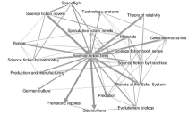
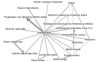
Figure 1: Two fragments of the latent category graph induced by LlamaFur matrix $W$, representing the 18 closest neighbors of categories “Science Fiction Films” and “Keyboardists”, respectively. The width of the arc from $c$ to $c^{\prime}$ is proportional to $w_{c,c^{\prime}}$, and arcs with $w_{c,c^{\prime}}\leq 1$ are not shown.

Let us now call $W$ the category matrix obtained at the end of the learning process (that is, $W=W_{T}$, according to the notation of Section 3), or equivalently the matrix built using the naive approach of Section 4. This matrix allows one to sort the links $(d,d^{\prime})\in L$ in increasing order of $\sum_{c\in C_{d_{t}}}\sum_{c^{\prime}\in C_{d_{t}^{\prime}}}w_{c,c^{\prime}}$ (i.e., by increasing explainability): the first links are the most unexpected.

In particular, in the case of the learning approach of Section 3, one can build a graph $G^{*}=(D,L^{*})$ whose links are the set $L^{*}$ of pairs $(d,d^{\prime})$ such that

$$\sum_{c\in C_{d_{t}}}\sum_{c^{\prime}\in C_{d_{t}^{\prime}}}w_{c,c^{\prime}}>0.$$

In a standard binary-classification scenario, $G^{*}$ would be the graph $G$ that our classifier learned. In particular, the elements of the set $L\setminus L^{*}$ ($L^{*}\setminus L$, resp.) are the false negative (false positive, resp.) instances.

But ours is not a link-prediction task, and we do not expect in any sense that $L$ and $L^{*}$ are similar. In particular, we shall certainly observe a phenomenon that we can call generalization effect: suppose that it frequently happens that a document assigned to a category $c$ (e.g., an actor) contains links to documents assigned to another category $c^{\prime}$ (e.g., a movie). This will probably make $w_{c,c^{\prime}}$ very large, and so we may falsely deduce that every document assigned to $c$ (every actor) contains a link to every document assigned to $c^{\prime}$ (every movie). In other words, LlamaFur cannot be used as a reliable link-prediction algorithm.

The generalization effect will, by itself, make $L^{*}$ much larger than $L$ (i.e., it will produce many false positive instances), but we do not care much about this aspect. Our focus is not on trying to reconstruct $L$, but rather in understanding which elements of $L$ are difficult to explain based on the categories of the involved documents. We say that a link $(d,d^{\prime})\in L$ is explainable iff $(d,d^{\prime})\in L^{*}$; the set of explainable links is therefore $L\cap L^{*}$. On the contrary, the elements of $L\setminus L^{*}$ are called unexplainable, and these are the links we want to focus on.

In Figure 1 we show two small examples of how the matrix $W$ learned as in Section 3 looks like, when considering the Wikipedia dataset (for a full explanation of how the dataset was built, see Section 6): in the picture, we display the 18 neighbours closer to two starting categories (“Science Fiction Films” and “Keyboardists”); the width of the arc from $c$ to $c^{\prime}$ is proportional to $w_{c,c^{\prime}}$, and arcs with $w_{c,c^{\prime}}\leq 1$ are not shown. For example, from the picture it is clear that a link from a page of a science-fiction film to a page of a science-fiction novel is highly expected, as it is one from a page of a keyboardist to one of a British progressive rock album. From this representations we can catch a glimpse of how this method is able to build a model for the graph, capturing meaningful relations between categories. The rougher version of the same neighborhood as induced by Naive-LlamaFur is shown in Figure 2: even from this small example, it is clear that the naive version introduces more noise (epitomized by the inclusion of “Language of the Carribean” and “Languages of Singapore” among the 18 closest neighbors of “Science fiction films”).

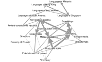
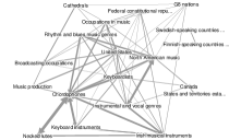
Figure 2: Two fragments of the latent category graph induced by Naive-LlamaFur matrix, representing the 18 closest neighbors of categories “Science Fiction Films” and “Keyboardists”, respectively. The width of the arc from $c$ to $c^{\prime}$ is proportional to $w_{c,c^{\prime}}$, and the lighter arcs are not shown. For comparison with LlamaFur, see Figure 1.

6 Experiments

Given its increasing importance in knowledge representation [42], we used the English edition of Wikipedia as our testbed. In particular, we employed the enwiki snapshot of February 3, 2014 to obtain:

• the document graph, composed by $4\,514\,662$ Wikipedia pages, with as many as $110\,699\,703$ arcs; every redirect was merged to its target page;

• the full categorization of pages: a map associating every page to one of the $1\,134\,715$ categories;

• the category pseudo-tree: a graph built by Wikipedia editors, with the aim of assigning each category to a “parent” category.

Wikipedia categories

The first problem is that the categorization on Wikipedia is quite noisy and, in fact, a continuous work-in-progress: categories may contain only one (or even no) page, they might be duplicates of each other, and so on. We therefore cleansed the page categorization using the methods described in [8]; in a nutshell, we computed the harmonic centrality measure [9] on the category hierarchy, and considered only the set $C$ of the $20\,000$ most central categories (called milestones). We chose $20\,000$ as a good compromise between the significance of these categories (in terms of the F-Measure of Alg. 1, see below) and the space needed to store $W$ (see Fig. 3).

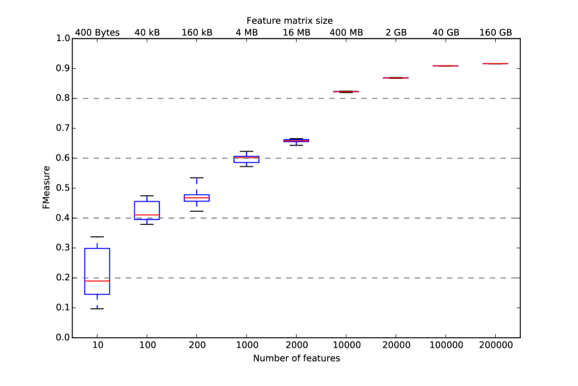
Figure 3: F-Measure of Alg. 1 in 10-fold cross-validation, with different number of considered categories. For each cardinality, we report the size required to store a dense representation of $W$.

We then computed, for every category $c$, the milestone $\iota(c)\in C$ closest to $c$ in the pseudo-tree (distances are computed as shortest paths in the pseudo-tree), and re-categorized all the pages applying $\iota(-)$ to its original categories. If there is no $c^{\prime}\in C$ connected to $c$, $\iota(c)$ is undefined and we simply discarded $c$.

At the end of the day, we obtained a set $C$ of $20\,000$ milestone categories, and a map associating each Wikipedia page $d$ to $C_{d}\subseteq C$; on average, each page belongs to $4$ categories. This cleansing process yields very clean labels; for instance, pages originally belonging to the category “Swiss manuscripts” are now categorized in “Swiss culture”, and similarly “Elections in Southwark” is remapped to “Local government in London”, “Flamenco compositions” to “Spanish music”, etc. Since the method we present is based on a well-defined categorization of labels, reducing the noise in the labels may be a key factor behind our results.

We proceeded then to apply LlamaFur to extract the latent category matrix $W$. In doing so, we first used a 10-fold cross-validation technique to assess how well Alg. 1 is generalizing; specifically, we divided in 10 folds the space of node pairs $D\times D$. The results, reported in Table 1, are consistent with our expectations, and suggest that we can consider the unexplained links as atypical. In particlar, the average of F-Measure on unknown node pairs is $86.9\%$, showing that the model learnt by LlamaFur is robust and not threatened by overfitting.

Measure	Results
Accuracy	$87.3\%\pm 0.06$
Precision	$90.0\%\pm 0.05$
Recall	$84.0\%\pm 0.14$
F-Measure	$86.9\%\pm 0.07$

Table 1: Average and standard deviation of results from a 10-fold cross-validation of Alg. 1 on the links of Wikipedia.

Learning on the whole graph, the ratio $|L\cap L^{*}|/|L|$ – that is, how many existing links are explained by $W$ – is equal to $86\%$. Please note that running our algorithm on the whole Wikipedia graph ($110\,699\,703$ arcs) and the categorization we chose ($20\,000$ categories) required only 9 minutes on an Intel Xeon CPU with 2.40GHz. We illustrated previously in Fig. 1 some fragments of $W$. Finally, we proceeded to assign our unexpectedness score to each link. An example of the largest and lowest scores for two Wikipedia articles is provided in Table 2 and 3.

Links of Jupiter
Most Unexpected		Most Expected
Inquisition	[Observation of Jupiter moons] was a major point in favor of Copernicus’ heliocentric theory of the motions of the planets; Galileo’s outspoken support of the Copernican theory placed him under the threat of the Inquisition.	Galileo Galilei	Galilean moons were first discovered by Galileo Galilei in 1610.
Proto-Indo-European language	[Jupiter] name comes from the Proto-Indo-European vocative compound *Dyeus-pater (nominative: *Dyeus-pater, meaning ”O Father Sky-God”, or ”O Father Day-God”).	E. E. Barnard	In 1892, E. E. Barnard [an American astronomer] observed a fifth satellite of Jupiter with the 36-inch (910 mm) refractor at Lick Observatory in California.
Gan De	Gan De, a Chinese astronomer, made the discovery of one of Jupiter’s moons in 362 BC with the unaided eye.	Ptolemy	[Ptolemy] constructed a geocentric planetary model based on deferents and epicycles to explain Jupiter’s motion relative to the Earth.
Fish	In 1976, before the Voyager missions, it was hypothesized that ammonia or water-based life could evolve in Jupiter’s upper atmosphere. This hypothesis is based on the ecology of terrestrial seas which have simple photosynthetic plankton at the top level, fish at lower levels feeding on these creatures, and marine predators which hunt the fish.	Jupiter (mythology)	The Romans named the planet after the Roman god Jupiter.

Table 2: Most expected and most unexpected links in the Wikipedia article Jupiter, according to LlamaFur.

Links of Kim Jong-il (supreme leader of North Korea from 1994 to 2011)
Most Unexpected		Most Expected
Elvis Presley	In a 2011 news story, The Sun reported Kim Jong-il was obsessed with Elvis Presley. His mansion was crammed with his idol’s records and his collection of 20,000 Hollywood movies included Presley’s titles – along with Rambo and Godzilla. He even copied the King’s Vegas-era look of giant shades, jumpsuits and bouffant hairstyle.	George W. Bush	Kim’s regime argued the secret [nuclear] production was necessary for security purposes – citing the presence of United States-owned nuclear weapons in South Korea and the new tensions with the United States under President George W. Bush.
Michael Jordan	Kim reportedly enjoyed basketball. Former United States Secretary of State Madeleine Albright ended her summit with Kim by presenting him with a basketball signed by NBA legend Michael Jordan.	Kim Il-sung	He succeeded his father and founder of the DPRK, Kim Il-sung.
Sonbong	[Kim Jong-il’s] father returned to Pyongyang that September, and in late November Kim returned to Korea via a Soviet ship, landing at Sonbong.	Adolf Hitler	A report […] concluded that the “big six” group of personality disorders shared by dictators Adolf Hitler, Joseph Stalin, and Saddam Hussein were also shared by Kim Jong-il.
Korean Air Flight 858	South Korea accused Kim of ordering the 1983 bombing in Rangoon, Burma which killed 17 visiting South Korean officials, including four cabinet members, and another in 1987 which killed all 115 on board Korean Air Flight 858.	Malta	Kim is also said to have received English language education at the University of Malta in the early 1970s.

Table 3: Most expected and most unexpected links in the Wikipedia article Kim Jong-il, according to LlamaFur.

Evaluation methodology

We want to evaluate the effectiveness of LlamaFur in mining unexpected links using a standard approach commonly adopted in Information Retrieval. In our context, a query is a document, the possible results are the hyperlinks that the document contains, and a result is relevant for our problem if it represents an unexpected link. The scenario we have in mind is that of a user wishing to find surprising links in a certain Wikipedia page. What we are trying to assess is how well LlamaFur can identify an unknown set of unexpected links, having full knowledge of graph and categorization of nodes.

In order to compare the results obtained by LlamaFur with the existing state-of-the-art for similar problems, we performed a user study based on the same pooling method adopted for many standard collections such as TREC (trec.nist.gov): we considered a random sample of 237 queries (i.e., Wikipedia documents); for each query we took, among its $t$ possible results (i.e., links), the top-$\left\lfloor{\alpha\cdot t}\right\rfloor$ most unexpected ones according to each system under comparison (see below); all the resulting links were evaluated by human beings. We set $\alpha=0.1$, and obtained about $3\,698$ links.

The human evaluators were asked to categorize each link into one of four classes (“totally expected”, “slightly expected”, “slightly unexpected” and “totally unexpected”). They were provided with the first paragraph of the two Wikipedia pages, and a link to the whole article if needed. The resulting dataset of $3\,698$ evaluated links is available for download and inspection. (To obtain a sufficiently large number of evaluated links in a short amount of time, there was virtually no overlap between the links that the evaluators worked on; however, we manually inspected the dataset to find that the labels produced are quite robust—we invite the reader to do the same.) After the human evaluation, we only considered the queries that have at least one irrelevant (“totally/slightly expected”) and one relevant (“totally/slightly unexpected”) result according to the evaluation, obtaining a dataset with $117$ queries. In this dataset, on average each query has $3.48$ relevant results over $20.9$ evaluated links. About $58.1\%$ of the links were labelled as “totally expected”, only $2.2\%$ were “totally unexpected” and about $8.8\%$ were labelled as “unexpected”.

It is evident how unexpected links are very sparse (many pages did not present any unexpected link at all); this motivated us to employ bpref [10], a well-suited information retrieval measure. To compute it, we followed TREC specifications; in a nutshell, bpref computes an index of how many judged relevant documents are retrieved ahead of judged non-relevant documents.

Baselines and competitors

In our comparison, LlamaFur is tested in combination and against a number of baselines and competitors. In particular, we considered LlamaFur and its naive variant, Naive-LlamaFur, along with some of the other (un)expectedness measures proposed in the literature.

Albeit there are, at the best of our knowledge, no algorithms specifically devoted to determining unexpected links, we can adapt some techniques used for unexpected documents to our case. All of those methods try to measure the unexpectedness of a document $d$ among a set of retrieved documents $R$. In our application, we are considering a link $(d^{\prime},d)$ and taking $R$ to be the set of all documents towards which $d^{\prime}$ has a hyperlink.

• Text-based methods. In the literature, all of the measures of unexpectedness are based on the textual content of the document under consideration.

  • The first index, called $\operatorname{M2}$ in [23] (a better variant of $M1$, the measure proposed in [28]), is defined as:

    $$\operatorname{M2}(d)=\frac{\sum_{t}U(d,t,R)}{m}$$

    where $m$ is the number of terms in the dictionary, and $U(d,t,R)$ is the maximum between 0 and the difference between the normalized term frequency of term $t$ in document $d$ and the normalized term frequency of $t$ in $R$ (the set of all retrieved documents). The normalized term frequency is the frequency of a term divided by the frequency of the most frequent term.

  • The second index, called $\operatorname{M4}$ in [23] (where they prove that it works better than $\operatorname{M2}$ in their context), is the

    $$\operatorname{M4}(d)=\max_{t}\operatorname{tf}(t)\cdot\log\frac{|R|}{\operatorname{df}(t)}$$

    where $\operatorname{tf}(t)$ is the normalized term frequency of term $t$ in $d$, and $\operatorname{df}(t)$ the number of documents in $R$ where $t$ appears.

• Link-prediction methods. A completely different, alternative approach to the problem is based on link prediction: how likely is it that the link $(d^{\prime},d)$ is created, if we assume that it is not there? Among the many techniques for link prediction [30], we tested the well-known Adamic-Adar index [1] ($\operatorname{AA}$, in the following), defined by

  $$\operatorname{AA}(d,d^{\prime})=\sum_{d^{\prime\prime}\in\Gamma(d)\cap\Gamma(d^{\prime})}\frac{1}{\log|\Gamma(d^{\prime\prime})|},$$

  where $\Gamma(d)$ is the set of documents which $d$ links to.

• Combinations. Besides testing all the described techniques in isolation, we tried to combine them linearly. Since each unexpectedness measure exhibits a different scale, we first need to normalize each measure by taking its studentized residual [14]. It is worth mentioning here that [21, 33] can also be used as link-prediction algorithms, and would apparently fit better our approach because they predict links based on binary node features, but the crucial difference is that in those models features are latent and need to be reconstructed, whereas in our scenario features (categories) are readily available.

Results

In the following, we are only going to discuss the best algorithms and combinations, besides some of the most interesting alternatives. The raw average bpref values are displayed in Table 4.

Algorithm	Average bpref	Input data
$\operatorname{AA}$	0.286	graph
$\operatorname{M2}$	0.179	bag of words
$\operatorname{M4}$	0.293	bag of words
Naive-LlamaFur	0.251	graph, categories
LlamaFur	0.343	graph, categories
LlamaFur + $\operatorname{AA}$	0.350	graph, categories

Table 4: Average values for bpref.

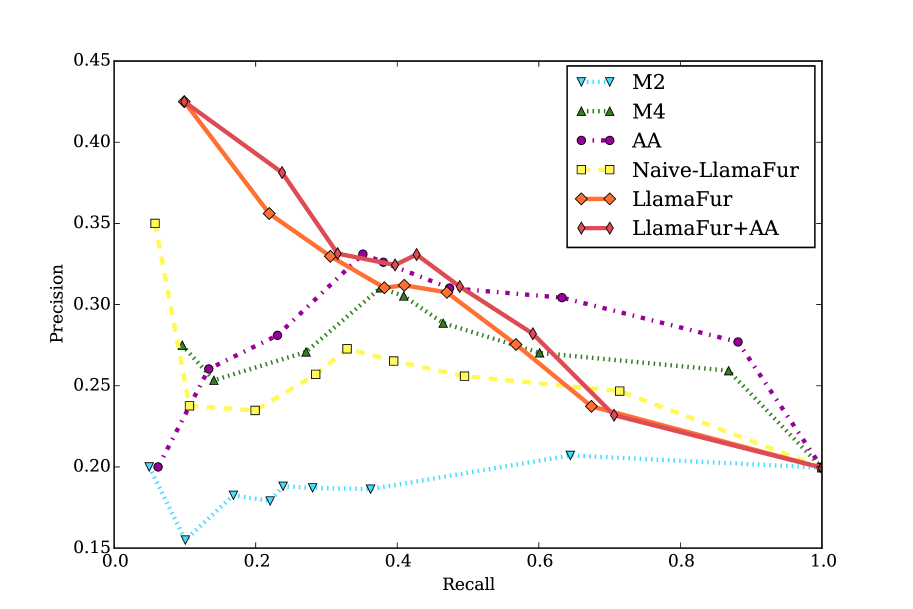
Figure 4: Average precision-recall values evaluated after the $1$st, $2$nd, $5$th, $8$th, $10$th, $15$th, $25$th, $50$th, and $100$th percentiles for each query.

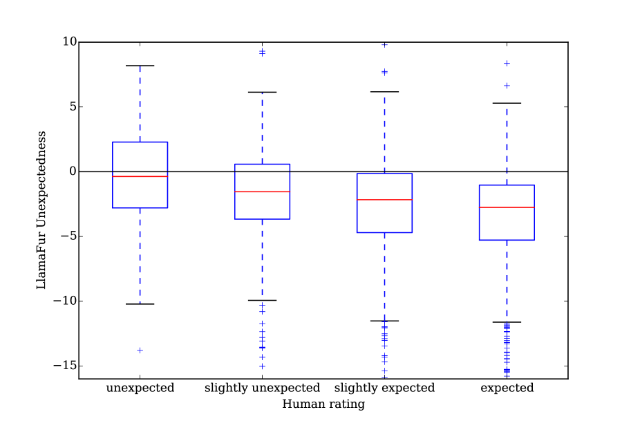
Figure 5: Comparison of the unexpectedness evaluated by LlamaFur with equation (1) over the different labels obtained from human evaluation.

Some complementary information about the behaviour is provided by the precision-recall graph of Figure 4: first of all, LlamaFur, $\operatorname{AA}$, $\operatorname{M4}$ and their combinations have larger precision than the remaining ones at almost all the recall levels; on the other hand LlamaFur +$\operatorname{AA}$ is the best method for recall values up to $50\%$, and LlamaFur has definitely better precision than $\operatorname{AA}$ until $30\%$ of recall.

In fact, $\operatorname{M4}$, $\operatorname{AA}$ and LlamaFur seem to be complementary to one another; in some sense, this is not surprising given that they stem from completely different sources of information: one is based on the textual content, another on the pure link graph and the latter on the category data.

Some further clue on the behaviour of LlamaFur is provided by Figure 5, where the distribution of LlamaFur expectedness values is shown for each of the four labels provided by the human evaluation. The red line is the median and the upper/lower hinge represent the 75th/25th percentile.

Finally, let us remark that in order to enhance reproducibility and to foster further research on this problem, we are sharing all code and data needed to replicate our findings on http://git.io/vmzjm.

7 Conclusions and future work

In this work we presented a graph model based on the interplay between categories, able to catch the notion of expected links on a graph; we showed that this model can be employed to find unexpected links in hyperlinked document corpora, through the determination of a latent category matrix; the latter is built using a perceptron-like technique. We demonstrated that our method provides better accuracy than most existing text-based techniques, with higher efficiency and relying on a much smaller amount of information. Moreover, we showed that LlamaFur can process graphs with $10^{8}$ links or more without effort. We carried out experiments on the categorized Wikipedia graph – a widely employed source of information for knowledge representation. It would be useful to try our unexpected link mining approach on a different graph, but we could not find any other openly-accessible dataset of expected/unexpected links.

An interesting question is whether the latent category matrix can be used to improve link prediction per se, i.e. if it is useful to find links and not only unexpected ones: this problem requires that one finds a way to bypass the generalization effect that the matrix produces (for example, by introducing stochastic behaviour in our model). Another possible direction would be to try different approach to the classification problem described in Section 3, in order to improve its effectiveness. To this aim, one could recast the problem as a cost-sensitive classification where false negatives are more costly than false positives. Other useful techniques include active learning [31]: since we need a subset of the non-linked pairs as counter-examples, active learning would select the more effective ones. An alternative approach to the same task would be to employ one-class learning [25]. This is left as future work.

Acknowledgments

Authors acknowledge the EU-FET grant NADINE (GA 288956). They also would like to thank Sebastiano Vigna, both for useful discussions and for providing some effective code to parse the Wikipedia snapshot.

References

- [1] L.A. Adamic and E. Adar. Friends and neighbors on the web. Social Networks, 25:211–230, 2001.
- [2] C.C. Aggarwal. Outlier analysis. Springer Science & Business Media, 2013.
- [3] M. Agyemang, K. Barker, and R. Alhajj. Hybrid approach to web content outlier mining without query vector. In A.M. Tjoa and J. Trujillo, editors, DaWaK, volume 3589 of Lecture Notes in Computer Science, pages 285–294. Springer, 2005.
- [4] S. O Aral, J.P. Hughes, B. Stoner, W. Whittington, H.H. Handsfield, R.M. Anderson, and K.K. Holmes. Sexual mixing patterns in the spread of gonococcal and chlamydial infections. American Journal of Public Health, 89(6):825–833, 1999.
- [5] H. Bisgin, N. Agarwal, and X. Xu. A study of homophily on social media. World Wide Web, 15(2):213–232, 2012.
- [6] C.M. Bishop. Pattern Recognition and Machine Learning (Information Science and Statistics). Springer-Verlag New York, Inc., 2006.
- [7] D.M. Blei, A.Y. Ng, and M.I. Jordan. Latent dirichlet allocation. JMLR, 3:993–1022, 2003.
- [8] P. Boldi and C. Monti. Cleansing wikipedia categories using centrality. In Proc. 24th International Conference on WWW, WWW ’16 Companion, 2016 (To appear).
- [9] P. Boldi and S. Vigna. Axioms for centrality. Internet Mathematics, 10(3-4):222–262, 2014.
- [10] C. Buckley and E.M. Voorhees. Retrieval evaluation with incomplete information. In Proc. of the 27th ACM SIGIR, pages 25–32. ACM, 2004.
- [11] V.R. Carvalho and W.W. Cohen. Single-pass online learning: Performance, voting schemes and online feature selection. In Proc. of the 12th ACM SIGKDD, pages 548–553. ACM, 2006.
- [12] J. Chang and D.M. Blei. Relational topic models for document networks. In International conference on artificial intelligence and statistics, pages 81–88, 2009.
- [13] D.G. Coderre. Fraud Detection: Using Data Analysis Techniques to Detect Fraud. Global Audit Publications, 1999.
- [14] R.D. Cook and S. Weisberg. Residuals and Influence in Regression. Monographs on Statistics and Applied Probability, 18. Chapman and Hall/CRC, 1983.
- [15] K. Crammer, O. Dekel, J. Keshet, S. Shalev-Shwartz, and Y. Singer. Online passive-aggressive algorithms. J. Mach. Learn. Res., 7:551–585, 2006.
- [16] Nello Cristianini and John Shawe-Taylor. An introduction to support vector machines and other kernel-based learning methods. Cambridge university press, 2000.
- [17] D. Eklou, Y. Asano, and M. Yoshikawa. How the web can help wikipedia: A study on information complementation of wikipedia by the web. In Proc. of the 6th International Conference on Ubiquitous Information Management and Communication, ICUIMC ’12, pages 9:1–9:10. ACM, 2012.
- [18] C. Gentile. A new approximate maximal margin classification algorithm. J. Mach. Learn. Res., 2:213–242, 2002.
- [19] K. Henderson and T. Eliassi-Rad. Applying latent dirichlet allocation to group discovery in large graphs. In Proc. 2009 ACM symposium on Applied Computing, pages 1456–1461. ACM, 2009.
- [20] N. Hens, N. Goeyvaerts, M. Aerts, Z. Shkedy, P. Van Damme, and P. Beutels. Mining social mixing patterns for infectious disease models based on a two-day population survey in belgium. BMC Infectious Diseases, 9(1):5, 2009.
- [21] P.D. Hoff. Multiplicative latent factor models for description and prediction of social networks. Computational and Mathematical Organization Theory, 15(4):261–272, 2009.
- [22] L. Isella, M. Romano, A. Barrat, et al. Close encounters in a pediatric ward: measuring face-to-face proximity and mixing patterns with wearable sensors. PloS one, 6(2):e17144, 2011.
- [23] F. Jacquenet and C. Largeron. Discovering unexpected documents in corpora. Knowledge-Based Systems, 22(6):421 – 429, 2009.
- [24] N. Japkowicz and S. Stephen. The class imbalance problem: A systematic study. Intelligent data analysis, 6(5):429–449, 2002.
- [25] S. S Khan and M.G. Madden. A survey of recent trends in one class classification. In Artificial Intelligence and Cognitive Science, pages 188–197. Springer, 2010.
- [26] M. Kim and J. Leskovec. Multiplicative attribute graph model of real-world networks. Internet Mathematics, 8(1-2):113–160, 2012.
- [27] S. Lattanzi and D. Sivakumar. Affiliation networks. In Proc. of the Forty-first Annual ACM Symposium on Theory of Computing, STOC ’09, pages 427–434, New York, NY, USA, 2009. ACM.
- [28] B. Liu, Y. Ma, and Philip S. Yu. Discovering unexpected information from your competitors’ web sites. In D. Lee, M. Schkolnick, F.J. Provost, and R. Srikant, editors, KDD, pages 144–153. ACM, 2001.
- [29] Y. Liu, A. Niculescu-Mizil, and W. Gryc. Topic-link lda: joint models of topic and author community. In Proc. 26th annual international conference on machine learning, pages 665–672. ACM, 2009.
- [30] L. Lü and T. Zhou. Link prediction in complex networks: A survey. Physica A: Statistical Mechanics and its Applications, 390(6):1150 – 1170, 2011.
- [31] E. Lughofer. Single-pass active learning with conflict and ignorance. Evolving Systems, 3(4):251–271, 2012.
- [32] M. McPherson, L. Smith-Lovin, and J.M. Cook. Birds of a feather: Homophily in social networks. Annual Review of Sociology, 27(1):415–444, 2001.
- [33] K.T. Miller, T.L. Griffiths, and M.I. Jordan. Nonparametric latent feature models for link prediction. In Y. Bengio, D. Schuurmans, J.D. Lafferty, C.K. I. Williams, and A. Culotta, editors, In NIPS, pages 1276–1284. Curran Associates, Inc., 2009.
- [34] C. Monti, A. Rozza, G. Zappella, M. Zignani, A. Arvidsson, and E. Colleoni. Modelling political disaffection from twitter data. In Proc. of the 2nd Int. WISDOM, page 3. ACM, 2013.
- [35] J. Mossong, N. Hens, M. Jit, et al. Social contacts and mixing patterns relevant to the spread of infectious diseases. PLoS Med, 5(3):e74, 2008.
- [36] T. Murakami, K. Mori, and R. Orihara. Metrics for evaluating the serendipity of recommendation lists. In Proc. of the 2007 Conf. on New Frontiers in Artificial Intelligence, JSAI’07, pages 40–46, Berlin, Heidelberg, 2008. Springer-Verlag.
- [37] A. Nadamoto, E. Aramaki, T. Abekawa, and Y. Murakami. Content hole search in community-type content. In Proc. of the 18th international conference on WWW, pages 1223–1224. ACM, 2009.
- [38] C. Plackner and V. Primoli. Data forensics: A compare-and-contrast analysis of multiple methods. In Proc. of the Conference on Statistical Detection of Potential Test Fraud, 2012.
- [39] S.P. Ponzetto and M. Strube. Deriving a large scale taxonomy from wikipedia. Proc. of the National Conference on Artificial Intelligence, 2, 2007.
- [40] N. Ramakrishnan and A.Y. Grama. Data mining-guest editors’ introduction: From serendipity to science. Computer, 32(8):34–37, 1999.
- [41] Stuart Russell and Peter Norvig. Artificial intelligence: A modern approach. 2010.
- [42] F.M. Suchanek, G. Kasneci, and G. Weikum. Yago: A large ontology from wikipedia and wordnet. Web Semantics: Science, Services and Agents on the World Wide Web, 6(3):203 – 217, 2008.
- [43] K. Tsukuda, H. Ohshima, M. Yamamoto, H. Iwasaki, and K. Tanaka. Discovering unexpected information on the basis of popularity/unpopularity analysis of coordinate objects and their relationships. In Proc. of the 28th Annual ACM Symposium on Applied Computing, SAC ’13, pages 878–885. ACM, 2013.