Local search yields approximation schemes for k-means and k-median in Euclidean and minor-free metrics

Abstract

We give the first polynomial-time approximation schemes (PTASs) for the following problems: (1) uniform facility location in edge-weighted planar graphs; (2) $k$-median and $k$-means in edge-weighted planar graphs; (3) $k$-means in Euclidean space of bounded dimension. Our first and second results extend to minor-closed families of graphs. All our results extend to cost functions that are the $p$-th power of the shortest-path distance. The algorithm is local search where the local neighborhood of a solution $S$ consists of all solutions obtained from $S$ by removing and adding $1/\varepsilon^{O(1)}$ centers.

1 Introduction

In this paper, we address three fundamental problems, facility location, $k$-median and $k$-means clustering, in two settings, graphs and Euclidean spaces. The problem of approximating $k$-means clustering in low-dimensional Euclidean space has been studied since at least 1994 [34]; since then, many researchers have given approximation schemes that are polynomial for fixed $k$ but exponential in $k$. Very recently, building on [22], a bicriteria polynomial-time approximation scheme has been given [15] for $k$-means: it finds $(1+\epsilon)k$ centers whose cost is at most $1+\epsilon$ times the cost of an optimal $k$-means solution. As the authors of that paper point out, it remained an open question whether there is a true polynomial-time approximation scheme for $k$-means in the plane (where $k$ is considered part of the input); the best polynomial-time approximation bound known was $9+\epsilon$. In this paper, we resolve this open question by giving the first polynomial-time approximation scheme for arbitrary (i.e. nonconstant) $k$ in low-dimensional Euclidean space.

Our analysis of the $k$-means approximation scheme shows that it can also be applied to graphs belonging to a fixed nontrivial minor-closed family.

For example, for any fixed integer $g$, graphs embeddable on a surface of genus $g$ form such a family. In particular, planar graphs forms such a family. Thus we also obtain the first polynomial-time approximation scheme for $k$-means in planar graphs.

The problems of (uncapacitated) metric facility location and $k$-median in graphs has similarly been studied for many years. The first polynomial-time approximation algorithm, with a logarithmic performance guarantee, was given by Hochbaum in 1982 [33]. The first polynomial-time approximation algorithm to achieve a constant approximation ratio was given by Shmoys et al.  [46] in 1997. It was later improved by Jain and Vazirani [36] and by Arya et al. [7]. The current best approximation algorithm for metric (uncapacitated) facility location, due to Li, has approximation ratio 1.488 [43]. Guha and Khuller  [27] proved that there exists no polynomial-time approximation algorithm with approximation ratio of 1.463 for metric facility location problem unless $NP\subseteq DTIME[n^{O(\log\log n)}]$. The current best approximation ratio for the $k$-median problem is $1+\sqrt{3}$ by Li and Svensson [44].

In order to obtain a substantially better approximation ratio, therefore, one must restrict attention to special metrics. Because facility location problems often arise on the surface of the earth, it is natural to consider the metrics induced by planar graphs. Researchers have been trying to find a polynomial-time approximation scheme for the planar restriction for many years. An unpublished manuscript [2] by Ageev dating back at least to 2001 addressed the planar case via a straightforward application of Baker’s method [12], giving an algorithm whose performance on an instance depends on how much of the cost of the optimal solution is facility-opening cost. Despite the title of the manuscript, the algorithm is not an approximation scheme for instances with arbitrary weights. Since then there have been no results on the problem despite efforts by several researchers in the area.

In this paper, we give the first polynomial-time approximation scheme for (uncapacitated uniform) facility location and $k$-median where the metric is that induced by a planar graph or, more generally a graph belonging to a fixed nontrivial minor-closed family.

1.1 Results

We describe a simple and natural, and previously studied local-search algorithm for clustering problems, parameterized by the desired cluster size $k$, the objective function $\text{cost}(\cdot)$, and a parameter $s$ governing the local-search neighborhood.

Algorithm 1 Local Search for finding $k$ clusters

1:Input: A metric space and associated cost function $\text{cost}(\cdot)$, an $n$-element set $C$ of points, error parameter $\varepsilon>0$, positive integer parameters $k$ and $s$

2:$S\leftarrow$ Arbitrary size-$k$ set of points

3:while $\exists$ $S^{\prime}$ s.t. $|S^{\prime}|\leq k$ and $|S-S^{\prime}|+|S^{\prime}-S|\leq s$ and cost($S^{\prime}$) $\leq$ $(1-\varepsilon/n)\text{cost}(S)$

4: do

5:     $S\leftarrow S^{\prime}$

6:end while

7:Output: $S$

We consider two kinds of metric spaces. For any fixed positive integer $d$, we consider $\mathbb{R}^{d}$ equipped with Euclidean distance. For any undirected edge-weighted graph $G$, we consider the metric completion of $G$, i.e. the metric space whose points are the vertices of $G$ and where the distance between $u$ and $v$ is defined to be the length of the shortest $u$-to-$v$ path in $G$ with respect to the given edge-weights.

Theorem 1.1 (Euclidean Spaces).

For any fixed integers $p,d>0$, there is a constant $c$ such that, for any $0<\varepsilon<1/2$, applying Algorithm 1 to the $d$-dimensional Euclidean space with cost function

$$\text{cost}(S)=\sum_{c\in C}(\min_{u\in S}\text{dist}(c,u))^{p}$$

and $s=1/\varepsilon^{c}$ yields a solution $S$ whose cost is at most $1+\varepsilon$ times the minimum.

When $p=2$, the objective function is the $k$-means objective function. When $p=1$, the objective function is that of $k$-median.

When the metric space is $\mathbb{R}^{d}$, it is not trivial to implement an iteration of Algorithm 1. However, as observed in [15] (see [34]), there is a method using an arrangement of algebraic surfaces to execute an iteration in $n^{O(ds)}$ time. The number of iterations is $O(n/\varepsilon)$ (see [7, 22]). The running time is therefore polynomial for fixed $p,d,\varepsilon$. We obtain the following.

Corollary 1.

For any integer $d>0$, there is a polynomial-time approximation scheme for the $k$-means problem in $d$-dimensional Euclidean spaces.

Algorithm 1 can also be applied to the metric completion of a graph.

Theorem 1.2 (Graphs).

Let $\mathcal{K}$ be a nontrivial minor-closed family of edge-weighted graphs. For any fixed integer $p>0$, there is a constant $c$ with the following property. For any $0<\varepsilon<1/2$, for any $G\in\mathcal{K}$, Algorithm 1 applied to the metric completion of $G$ with cost function

$$\text{cost}(S)=\sum_{c\in C}(\min_{u\in S}\text{dist}(c,u))^{p}$$

and with $s=1/\varepsilon^{c}$ yields a solution $S$ whose cost is at most $1+\varepsilon$ times the minimum.

It is straightforward to implement Algorithm 1 applied to the metric completion of a graph. As before, the number of iterations is $O(n/\varepsilon)$ where $n$ is the number of clients. We therefore obtain:

Corollary 2.

There is a polynomial-time approximation scheme for $k$-means and for $k$-median in planar graphs and in bounded-genus graphs.

More generally, for any nontrivial minor-closed family of edge-weighted graphs, there is a polynomial-time approximation schemes for $k$-means and for $k$-median for graphs in that family.

The local-search algorithm is easily adapted to the case where we do not specify the number of clusters but instead specify a per-cluster cost. This case includes a variant of the facility location problem.

Definition 1.1 (Uncapacitated Uniform Facility Location).

The Uncapacitated Uniform Facility Location problem is as follows: given a finite metric space, a subset $C$ of points, and a facility opening cost $f$, find a subset $S$ of points that minimizes $\text{cost}(S)=f|S|+\sum_{c\in C}\min_{u\in S}\text{dist}(c,u)$.

To address this problem, we use a simple modification of the local-search algorithm given earlier.

Algorithm 2 Local Search for Uniform Facility Location

1:Input: A metric space and associated cost function $\text{cost}(\cdot)$, an $n$-element set $C$ of points, error parameter $\varepsilon>0$, facility opening cost $f>0$, positive integer parameter $s$

2:$S\leftarrow$ Arbitrary subset of $\mathcal{F}$.

3:while $\exists$ $S^{\prime}$ s.t. $|S-S^{\prime}|+|S^{\prime}-S|\leq s$ and cost($S^{\prime}$) $\leq$ $(1-\varepsilon/n)$ cost($S$)

4: do

5:     $S\leftarrow S^{\prime}$

6:end while

7:Output: $S$

Theorem 1.3.

Fix a nontrivial minor-closed family $\mathcal{K}$ of graphs. There is a constant $c$ such that, when Algorithm 2 is applied to the metric completion of a graph in $\mathcal{K}$ with

$$\text{cost}(S)=|S|f+\sum_{c\in C}(\min_{u\in S}\text{dist}(c,u))^{p}$$

and $s=1/\varepsilon^{c}$, the output has cost at most $1+\varepsilon$ times the minimum.

In fact, for $p=1$, setting $s=c/\varepsilon^{2}$ suffices to achieve a $1+\varepsilon$ approximation. The theorem implies the following:

Corollary 3.

Fix a nontrivial minor-closed family $\mathcal{K}$ of edge-weighted graphs. There is a polynomial-time approximation scheme for uniform uncapacitated facility location in graphs of $\mathcal{K}$.

1.2 Related work

In arbitrary metric spaces, it is NP-hard to approximate the $k$-median and $k$-means problems within a factor of $1+2/e$ and $1+3/e$ respectively, see Guha and Khuller [27] and Jain et al. [35]. In the case of Euclidean space, Guruswami and Indyk [29] showed that there is no PTAS for $k$-median if both $k$ and $d$ are part of the input. More recently, Awasthi et al. [9] showed APX-Hardness for $k$-means if both $k$ and $d$ are part of the input.

In Euclidean spaces, $(1+\varepsilon)$-approximation algorithms for $k$-median have been proposed when $k$ or $d$ is fixed. For example, when $k$ is fixed, there exists different PTAS (See [11, 41, 42, 24, 31] and  [23] for the best known so far). When $d$ is fixed, Arora et al. gave the first PTAS [4] for the $k$-median problem. This result was subsequently improved to an efficient PTAS by Kolliopoulos et al. [38] and Har-Peled et al. [30, 31].

For the $k$-means problem, Kanungo et al. [37] showed that local search achieves a $9+\varepsilon$-approximation in general metrics and this remains the best known approximation guarantee so far even for fixed $d$. There are also a variety of results for $k$-means and $k$-median when the input has some stability conditions (see for example [10, 8, 14, 13, 18, 40, 45]) or in the context of smoothed analysis (see for example [6, 5]).

Local Search for metric $k$-median was first analyzed by Korupolu et al [39]. They gave a bicriteria approximation using $k\cdot(1+\varepsilon)$ centers an achieving a cost of at most $3+5/\varepsilon$ times the cost of the optimum $k$-clustering. This was later improved to $k\cdot(1+\varepsilon)$ centers an achieving a cost of at most $2+2/\varepsilon$ times the cost of the optimum $k$-clustering by Charikar an Guha [21]. Arya et al. [7] gave the first analysis showing that Local Search with a neighborhood of size $1/\varepsilon$ gives a $3+2\varepsilon$ approximation to $k$-median. Moreover, they show that this bound is tight. As mentioned earlier, Kanungo et al. [37] showed that local search is a $9+\varepsilon$-approximation for $k$-means in general metrics. Local search is a very popular algorithm for clustering and has been widely used : see [19] in the context of parallel algorithms,  [28] in the streaming model and  [16] for distributed computing. See [1] for a general introduction to theory and practice of local search.

Note added:

After we had written up our results and while we were editing the submission, we noticed a recent ArXiv paper [26] that has similar results for doubling metrics.

2 Techniques

2.1 $r$-divisions in minors

One key ingredient in our analyses is the existence of a certain kind of decomposition of the input called a weak $r$-division. The concept (in a stronger form) is due to Frederickson [25] in the context of planar graphs. It is straightforward to extend it to any family of graphs with balanced separators of size sublinear-polynomial. We also define a weak $r$-division for points in a Euclidean space, and show that such a decomposition always exists. These definitions and results are in Sections 3.1 and 3.2. Note that $r$-divisions play no role in our algorithm; only the analysis uses them.

Chan and Har-Peled [20] showed that local search can be used to obtain a PTAS for (unweighted) maximum independent pseudo-disks in the plane, which implies the analogous result for planar graphs. More generally, Har-Peled and Quanrud [32] show that local search can be used to obtain PTASs for several problems including independent set, set cover, and dominating set, in graphs with polynomial expansion. These graphs have small separators and therefore $r$-divisions. However, our analysis of local search for clustering requires not only that the input graph have an $r$-division but that a minor of the input graph have an $r$-division. This is not true of graphs of polynomial expansion. Indeed, we show in Section 2.3 that there are low-density graphs in low-dimensional space (which are therefore polynomial-expansion graphs) for which our local-search algorithm produces a solution that is worse than the optimum by at least a constant factor.

Thus one of our technical contributions is showing how to take advantage of a property possessed by nontrivial minor-closed graph families that is not possessed by polynomial-expansion graph families.

2.2 Isolation

In order to obtain our approximation schemes for $k$-means and $k$-median clustering, we need another technique. As mentioned earlier, a bicriteria approximation scheme for $k$-means was already known; the solution it returns has more than $k$ centers. It seems hard to avoid an increase in the number of centers in comparing a locally optimal solution to a globally optimal solution. It would help if we could show that the globally optimal solution could be modified so as to reduce the number of centers below $k$ while only slightly increasing the cost; we could then compare the local solution to this modified global solution, and the increase in the number of centers would leave the number no more than $k$.

Unfortunately, we cannot unconditionally reduce the number of centers. However, consider a globally optimal solution $\mathcal{G}$ and a locally optimal solution $\mathcal{L}$. A facility $f$ in $\mathcal{G}$ might correspond to a facility $\ell$ in $\mathcal{L}$ in the sense that they serve almost exactly the same set of clients. In this case, we say the pair $(f,\ell)$ is 1-1 isolated (the formal definition is below). Such centers do not contribute much to the increase in cost in going from global solution to local solution, so let’s ignore them. Among the remaining centers of $\mathcal{G}$, there are a substantial number that can be removed without the cost increasing much. The analysis of the local solution then proceeds as discussed above.

We now give the formal definition of 1-1 isolated.

Definition 2.1.

Let $\varepsilon<1/2$ be a positive constant and $\mathcal{L}$ and $\mathcal{G}$ be two solutions for the $k$-clustering problem with parameter $p$. Given a facility $f_{0}\in\mathcal{G}$ and a facility $\ell\in\mathcal{L}$, we say that the pair $(f,\ell)$ is 1-1-isolated if most of the clients served by $\ell$ in $\mathcal{L}$ are served by $f$ in $\mathcal{G}$, and most of the clients served by $f$ in $\mathcal{G}$ are served by $\ell$ in $\mathcal{L}$ : in other words,

$$|V_{\mathcal{L}}(\ell)\cap V_{\mathcal{G}}(f)|\geq\left\{\begin{array}[]{l}(1-\varepsilon)|V_{\mathcal{L}}(\ell)|\\ (1-\varepsilon)|V_{\mathcal{G}}(f)|\end{array}\right.$$

Theorem 2.2.

Let $\varepsilon<1/2$ be a positive constant and $\mathcal{L}$ and $\mathcal{G}$ be two solutions for the $k$-clustering problem with exponent $p$. Let $\bar{k}$ denote the number of facilities $f$ of $\mathcal{G}$ that are not in a 1-1 isolated region. There exists a set $S_{0}$ of facilities of $\mathcal{G}$ of size at least $\varepsilon^{3}\bar{k}/6$ that can be removed from $\mathcal{G}$ at low cost: $\text{cost}(\mathcal{G}-S_{0})\leq(1+2^{3p+1}\varepsilon)\text{cost}(\mathcal{G})+2^{3p+1}\varepsilon\text{cost}(\mathcal{L})$.

Note that the following theorem does not assume that $\mathcal{L}$ is a local optimum and $\mathcal{G}$ is an optimal solution. Thus we believe that this theorem can be of broader interest. We now define the concept of isolated regions; 1-1-isolated regions correspond to the special case of isolated regions when $\mathcal{L}_{0}$ consists of a single facility.

Definition 2.1 (Isolated Region).

Given a facility $f_{0}\in\mathcal{G}$ and a set of facilities $\mathcal{L}_{0}\subseteq\mathcal{L}$, we say that the pair $(f_{0},\mathcal{L}_{0})$ is an isolated region if

• For each facility $f^{\prime}\in\mathcal{L}_{0}$, most of the clients served by $f^{\prime}$ in $\mathcal{L}$ are served by $f_{0}$ in $\mathcal{G}$: in other words, $|V_{\mathcal{L}}(f^{\prime})\cap V_{\mathcal{G}}(f_{0})|\geq(1-\varepsilon)|V_{\mathcal{L}}(f^{\prime})|$, and

• Most of the clients served by $f_{0}$ in $\mathcal{G}$ are served by facilities of $\mathcal{L}_{0}$ in $\mathcal{L}$: in other words, $|V_{\mathcal{L}}(\mathcal{L}_{0})\cap V_{\mathcal{G}}(f_{0})|\geq(1-\varepsilon)|V_{\mathcal{G}}(f_{0})|$;

Finally, if $(f_{0},\mathcal{L}_{0})$ is an isolated region, we say that $f_{0}$ and the elements of $\mathcal{L}_{0}$ are isolated.

2.3 Tightness of the results

Proposition 2.3.

For any $w,t$, there exists an infinite family of graphs excluding $K_{w}$ as a $t$-shallow minor such that for any constant $\varepsilon$, local search with neighborhoods of size $1/\varepsilon$ might return a solution of cost at least $3\text{OPT}$.

See Figure 1 and [7] for a complete proof that local search performs badly on the instance depicted in the figure.

Proposition 2.4.

For any $\rho$, there exists an infinite family of graphs that are low-density graphs such that for any constant $\varepsilon$, local search with neighborhoods of size $1/\varepsilon$ might return a solution of cost at least $3\text{OPT}$.

The proposition follows from encoding the graph of Figure 1 as an low-density graph.

We additionally remark that Awasthi et al. [9] show that the $k$-means problem is APX-Hard for any non-constant dimension $d$. Moreover, Kanungo et al. [37] give an example where local search returns a solution of cost at least $9\text{OPT}$.

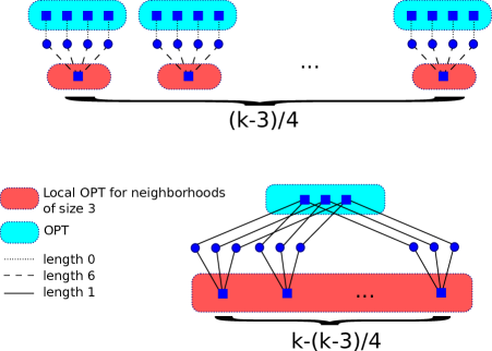
Figure 1: This instance contains the complete bipartite graph $K_{3,3}$ as a 1-shallow minor (and so is not planar) but no non-trivial 0-shallow minor. Clients are denoted by circle and candidate centers by squares. There exists a local (for neighborhoods of size 3) optimum whose cost is at least $3\text{OPT}$. This example can be generalized to handle locality for neighborhoods of size $1/\varepsilon$ for any constant $\varepsilon>0$. This is based on an example of [7] and can be extended to form a $i$-shallow minor graph for any $i=o(n)$.

3 Preliminaries

We will use the following technical lemma in order to give a general proof that encompasses both the cases of $k$-median and $k$-means. Throughout the paper we assume $p$ constant and define $\varepsilon_{1}$ to be a positive constant.

Lemma 3.1.

Let $p\geq 0$ and $0<\varepsilon_{1}<1/2$. For any $a,b,c\in A\cup F$, we have

$$\text{dist}(a,b)^{p}\leq\begin{cases}(1+\varepsilon_{1})^{p}(\text{dist}(a,c)^{p}+\text{dist}(c,b)^{p}/\varepsilon_{1}^{p})\\ 2^{p}(\text{dist}(a,c)^{p}+\text{dist}(c,b)^{p}).\end{cases}$$

Proof.

By the triangular inequality,

$$\text{dist}(a,b)^{p}=(\text{dist}(a,c)+\text{dist}(c,b))^{p}\leq\begin{cases}(1+\varepsilon_{1})^{p}\text{dist}(a,c)^{p}&\mbox{If $\text{dist}(c,b)\leq\varepsilon_{1}\text{dist}(a,c)$.}\\ (1+\varepsilon_{1})^{p}\text{dist}(c,b)^{p}/\varepsilon^{p}_{1}&\mbox{Otherwise.}\\ \end{cases}$$

Moreover, by the binomial theorem, $\text{dist}(a,b)^{p}=(\text{dist}(a,c)+\text{dist}(c,b))^{p}\leq 2^{p}(\text{cost}(a,c)^{p}+\text{cost}(c,b)^{p}).$ ∎

3.1 Graph $r$-division and other definitions

For a graph $G$, we use $V(G)$ and $E(G)$ to denote the set of vertices of $G$ and the set of edges of $G$, respectively. For a subgraph $H$ of $G$, the vertex boundary of $H$ in $G$, denoted $\partial_{G}(H)$, is the set of vertices $v$ such that $v$ is in $H$ but has an incident edge that is not in $H$. (We might write $\partial(H)$ if $G$ is unambiguous.) A vertex in the vertex boundary of $H$ is called a boundary vertex of $H$. A vertex of $H$ that is not a boundary vertex of $H$ is called an internal vertex. We denote the set of internal vertices of $H$ as $\mathcal{I}(H)$.

Definition 3.2.

Let $c_{1}$ and $c_{2}$ be constants (depending on $\mathcal{G}$). For a number $r$, a weak $r$-division of a graph $G$ (with respect to $c_{1},c_{2}$) is a collection $\mathcal{R}$ of subgraphs of $G$, called regions, with the following properties.

1. Each edge of $G$ is in exactly one region.

2. The number of regions is at most $c_{1}|V(G)|/r$.

3. Each region contains at most $r$ vertices.

4. The number of boundary vertices, summed over all regions, is at most $c_{2}|V(G)|/r^{1/2}$.

A family of graphs $F$ is said to be closed under taking minor (minor-closed) if for any graph $G\in F$, for any minor $H$ of $G$, we have $H\in F$.

Theorem 3.3 (Frederickson [25] + Alon, Seymour, and Thomas [3]).

Let $\mathcal{K}$ be a nontrivial minor-closed family of graphs. There exist $c_{1},c_{2}$ such that every graph in $\mathcal{K}$ has a weak $r$-division with respect to $c_{1},c_{2}$.

Proof.

Alon, Seymour, and Thomas  [3] proved a separator theorem for the family of graphs excluding a fixed graph as a minor. Any nontrivial minor-closed family excludes some graph as a minor (else it is trivial). Frederickson [25] gave a construction for a stronger kind of $r$-division of a planar graph. The construction uses nothing of planar graphs except that they have such separators. ∎

Let $G$ be an undirected graph with edge-lengths. Fix an arbitrary priority ordering of the vertex set $V(G)$. For every subset $S$ of $V(G)$, we define the Voronoi partition with respect to $S$. For each vertex $v\in S$, the Voronoi cell with center $v$, denoted $V_{S}(v)$, is the set of vertices that are closer to $v$ than to any other vertex in $S$, breaking ties in favor of the highest-priority vertex of $S$.

Fact 1.

For any $S$, for any vertex $v\in S$, the induced subgraph $G[V_{S}(v)]$ is a connected subgraph of $G$.

Proof.

Let $u\in V_{S}(v)$, and let $p$ denote a $v$-to-$u$ shortest path. Let $w$ be a vertex on $P$. Assume for a contradiction that, for some vertex $v^{\prime}\in S$, either the $v^{\prime}$-to-$w$ shortest path $p^{\prime}$ is shorter than the shortest $v$-to-$w$ path, or it is no longer and $v^{\prime}$ has higher priority than $v$. Replacing the $v$-to-$w$ subpath of $p$ with $p^{\prime}$ yields a $v$-to-$u$ path that either is shorter than $p$ or is no longer than $p$ and originates at a higher-priority vertex than $v$. ∎

It follows that, for any vertex $v$ of $G$, contracting the edges of the subgraph $G[V_{S}(v)]$ yields a single vertex.

Definition 3.4.

We define $G_{\text{Vor}(S)}$ as the graph obtained from $G$ by contracting every edge of $G[V_{S}(v)]$ for every vertex $v\in S$. For each vertex $v\in S$, we denote by $\hat{v}$ the vertex of $G_{\text{Vor}(S)}$ resulting from contracting every edge of $G[V_{S}(v)]$.

If $G$ belongs to a minor-closed family $\mathcal{K}$ then so does $G_{\text{Vor}(S)}$.

3.2 Euclidean space $r$-division

We define analogous notions for the case of Euclidean spaces of fixed dimension $d$. Consider a set of points $C$ in $\mathbb{R}^{d}$. For a set $Z$ of points in $\mathbb{R}^{d}$ and a bipartition $C_{1}\cup C_{2}$ of $C$, we say that $Z$ separates $C_{1}$ and $C_{2}$ if, in the Voronoi diagram of $C\cup Z$, the boundaries of cells of points in $C_{1}$ are disjoint from the boundaries of cells of points in $C_{2}$.

Definition 3.5.

Let $c_{1}$ and $c_{2}$ be constants. Let $C$ be a set of points in $\mathbb{R}^{d}$. For an integer $r>1$, a weak $r$-division of $C$ (with respect to $c_{1},c_{2}$) is a set of boundary points $Z\subset\mathbb{R}^{d}$ together with a collection of subsets $\mathcal{R}$ of $C\cup Z$ called regions, with the following properties.

1. ${\mathcal{R}}-Z$ is a partition of $C$.

2. The number of regions is at most $c_{1}|C|/r$.

3. Each region contains at most $r$ points of $C\cup Z$.

4. $\sum_{R\in\mathcal{R}}|R\cap Z|\leq c_{2}|C|/r^{1/d}$.

Moreover, for any region $R_{i}$, $R_{i}\cap Z$ is a Voronoi separator for $R_{i}-Z$ and $(C\cup Z)-R_{i}$.

The following theorem is from [17, Theorem 3.7].

Theorem 3.6.

[17, Theorem 3.7] Let $P$ be a set of $n$ points in $\mathbb{R}^{d}$. One can compute, in expected linear time, a sphere $S$, and a set $Z\subseteq S$, such that

• $|Z|\leq cn^{1-1/d}$,

• There are most $\sigma n$ points of $P$ in the sphere $S$ and at most $\sigma n$ points of $P$ not in $S$, and

• $Z$ is a Voronoi separator of the points of $P$ inside $S$ from the points of $P$ outside $S$.

Here $c$ and $\sigma<1$ are constants that depends only on the dimension $d$.

From that theorem we can easily derive the following (see Section 8.1 for the proof):

Theorem 3.7.

Let $r$ be a positive integer and $d$ be fixed. Then there exist $c_{1},c_{2}$ such that every set of points $C\subset\mathbb{R}^{d}$ has a weak $r$-division with respect to $c_{1},c_{2}$.

3.3 Properties of the $r$-Divisions

We present the properties of the $r$-divisions that we will be using for the analysis of the solution output by the local search algorithm.

Lemma 3.8.

Let $G=(V,E)$ be a graph excluding a fixed minor $H$ and $\mathcal{F}\subseteq V$. Let $H_{i}$ be a region of the $r$-division of $G_{\text{Vor}(\mathcal{F})}$. Suppose $c$ and $v$ are vertices of $G$ such that one of the vertices in $\{\hat{c},\hat{v}\}$ is a vertex of $H_{i}$ and the other is not an internal vertex of $H_{i}$. Then there exists a vertex $x\in\mathcal{F}$ such that $\hat{x}$ is a boundary vertex of the region $H_{i}$ and $\text{dist}(c,x)\leq\text{dist}(c,v)$.

Proof.

Let $p$ be a shortest $c$-to-$v$ path in $G$. By the conditions on $\hat{c}$ and $\hat{v}$, there is some vertex $w$ of $p$ such that $\hat{w}$ is a boundary vertex of $H_{i}$. Let $x$ be the center of the Voronoi cell whose contraction yields $\hat{w}$. By definition of Voronoi cell, $\text{dist}(w,x)\leq\text{dist}(w,v)$. Therefore replacing the $w$-to-$v$ subpath of $p$ with the shortest $w$-to-$x$ path yields a path no longer than $p$. ∎

We obtain the analogous lemma for the Euclidean case, whose proof follows directly from the definition of $r$-division (i.e.: the fact that $Z$ is a Voronoi separator).

Lemma 3.9.

Let $C$ be a set of points in $\mathbb{R}^{d}$ and $Z$ be an $r$-division of $C$. For any two different regions $R_{1},R_{2}$, for any points $c\in R_{1},v\in R_{2}$ there exists a boundary vertex $x\in Z\cap R_{1}$ such that $\text{dist}(c,x)\leq\text{dist}(c,v)$.

4 Facility Location in minor-closed graphs: Proof of Theorem 1.3

As a warm-up, we analyze Local Search for Uniform Facility Location (Algorithm 2) applied to the metric completion of an edge-weighted graph $G$ belonging to a nontrivial minor-closed family $\mathcal{K}$. The proof of the $k$-median and $k$-means results (for both Euclidean and minor-closed metrics), involve the use of Theorem 2.2 and a more complex analysis.

Throughout this section we consider a solution $\mathcal{L}$ output by Algorithm 2 (the “local” solution) and a globally optimal solution $\mathcal{G}$ of value OPT. Let $\mathcal{F}=\mathcal{L}\cup\mathcal{G}$. Let $r=1/\varepsilon^{2}$. Consider the graph $G_{\text{Vor}(\mathcal{F})}$ defined in Definition 3.4, and recall that each vertex of $G$ maps to a vertex $\hat{v}$ in the contracted graph $G_{\text{Vor}(\mathcal{F})}$.

Since $G$ belongs to $\mathcal{K}$ and $G_{\text{Vor}(\mathcal{F})}$ is obtained from $G$ by contraction, it too belongs to $\mathcal{K}$ and hence it has an $r$-division. Let $H_{1},\ldots H_{\kappa}$ be the regions of this $r$-division. For $i=1,\ldots,\kappa$, define $V_{i}$ and $B_{i}$ as follows:

$$V_{i} = \{v\in\mathcal{F}\ :\ \hat{v}\text{ is a vertex of }H_{i}\}$$

$$B_{i} = \{v\in\mathcal{F}\ :\ \hat{v}\text{ is a boundary vertex of }H_{i}\}$$

That is, $V_{i}$ is the set of vertices in the union of the local solution and the global solution that map via contraction to vertices of the region $H_{i}$, and $B_{i}$ is the set of vertices in the union that map to boundary vertices of $H_{i}$.

Let $\mathcal{G}^{\prime}=\mathcal{G}\cup\bigcup_{i=1}^{\kappa}B_{i}$.

Fix a region $H_{i}$ of the $r$-division of $G_{\text{Vor}(\mathcal{F})}$. We define $\mathcal{L}_{i}=\mathcal{L}\cap V_{i}$ and $\mathcal{G}^{\prime}_{i}=\mathcal{G}^{\prime}\cap V_{i}$. We consider the mixed solution $\mathcal{M}^{i}$ defined as follows:

$$\mathcal{M}^{i}=(\mathcal{L}-\mathcal{L}_{i})\cup\mathcal{G}^{\prime}_{i}.$$

Lemma 4.1.

$|\mathcal{M}^{i}-\mathcal{L}|+|\mathcal{L}-\mathcal{M}^{i}|\leq 1/\varepsilon^{2}$.

Proof.

To obtain $\mathcal{M}^{i}$ from $\mathcal{L}$, one can remove the vertices in $\mathcal{L}\cap V_{i}$ that are not in $\cal G^{\prime}$, and add the vertices in ${\cal G^{\prime}}\cap V_{i}$ that are not in $\mathcal{L}$. Thus the size of the symmetric difference is at most $|(\mathcal{L}\cup\mathcal{G}^{\prime})\cap V_{i}|$. Since the vertices of $\mathcal{L}\cup\mathcal{G}^{\prime}$ are centers of Voronoi cells, these vertices all map to different vertices in the contracted graph $G_{\text{Vor}(\mathcal{F})}$. Therefore $|(\mathcal{L}\cup\mathcal{G}^{\prime})\cap V_{i}|$ is at most the number of vertices in region $H_{i}$, which is at most $r=1/\varepsilon^{2}$. ∎

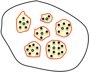
Figure 2: The diagram shows a region of the weak $r$-division. The blobs represent vertices of the region. Each blob is obtained by coalescing a set of vertices of the input graph. These vertices are indicated by circles. The unfilled circled represent the centers of the Voronoi cells.

Lemma 4.2.

Let $c$ be a vertex of $G$ and $H_{i}$ a region. Then:

$$m_{c}^{i}-l_{c}\leq\begin{cases}g_{c}-\ell_{c}&\mbox{if $\hat{c}$ is an internal vertex of $H_{i}$}\\ 0&\mbox{otherwise.}\\ \end{cases}$$

Proof.

First suppose $\hat{c}$ is an internal vertex of $H_{i}$, and let $v$ be the facility in $\mathcal{M}^{i}$ closest to $c$. If $v$ is in $V_{i}$ then it is in $\mathcal{G}_{i}$, so $m_{c}^{i}=g^{\prime}_{i}$. Suppose $v$ is not in $V_{i}$. Then by Lemma 3.8 there is a vertex $x\in\mathcal{F}$ such that $\hat{x}$ is a boundary vertex of $H_{i}$ and $\text{dist}(c,x)\leq\text{dist}(c,v)$. As before, $x$ is in $\mathcal{G}^{\prime}_{i}$ so $m_{c}^{i}\leq g^{\prime}_{c}$. Since $g^{\prime}_{c}\leq g_{c}$, this proves the claimed upper bound.

Now, suppose $\hat{c}$ is not an internal vertex of $H_{i}$ and let $v$ be the facility in $\mathcal{L}$ closest to $c$. If $v$ is not in $V_{i}$ then it is in the mixed solution $\mathcal{M}^{i}$, so $m_{c}^{i}=\ell_{c}$. Suppose $v$ is in $V_{i}$. Then by Lemma 3.8 there is a vertex $x\in\mathcal{F}$ such that $\hat{x}$ is a boundary vertex of $H_{i}$ and $\text{dist}(c,x)\leq\text{dist}(c,v)$. Since $x$ is in $\mathcal{F}$ and $\hat{x}$ is a boundary vertex of $H_{i}$, we know $x$ is in $\mathcal{G}^{\prime}\cap V_{i}$, which is $\mathcal{G}^{\prime}_{i}$. Therefore $x$ is in $\mathcal{M}^{i}$. Since $\text{dist}(c,x)\leq\text{dist}(c,v)$, we obtain $m_{c}^{i}\leq\ell_{c}$, which proves the claimed upper bound. ∎

Lemma 4.3.

$$\sum_{i=1}^{\kappa}|\mathcal{G}^{\prime}_{i}|\leq|\mathcal{G}|+c_{2}\varepsilon(|\cal G|+|\mathcal{L}|)$$

Proof.

Let $v$ be a vertex of $\mathcal{G}^{\prime}$. For $i=1,\ldots,\kappa$, if $\hat{v}$ is an internal vertex of the region $H_{i}$ then $v$ contributes only one towards the left-hand side. If $\hat{v}$ is a boundary vertex of $H_{i}$ then $v\in B_{i}$. Therefore

$$\sum_{i=1}^{\kappa}|\mathcal{G}^{\prime}\cap V_{i}|\leq|\mathcal{G}|+\sum_{i=1}^{\kappa}|B_{i}|.$$

To finish the proof, we bound the sum in the right-hand side. Each vertex in $\mathcal{F}$ is the center of one Voronoi cell, so $G_{\text{Vor}(\mathcal{F})}$ has $|\mathcal{F}|$ vertices. For each region $H_{i}$, there is one vertex in $B_{i}$ that corresponds to each boundary vertex of $H_{i}$, so $\sum_{i=1}^{\kappa}|B_{i}|$ is the sum over all regions of the number of boundary vertices of that region, which, by Property 4 of $r$-divisions, is at most $c_{2}|\mathcal{F}|/r^{1/2}$, which, by choice of $r$, is at most $c_{2}\varepsilon|{\cal F}|$, which in turn is at most $c_{2}\varepsilon(|{\cal G}|+|\mathcal{L}|)$.

∎

Proof.

(Proof of Theorem 1.3) Lemma 4.1 and the stopping condition of Algorithm 2 imply the following:

$$-{1\over n}\text{cost}(\mathcal{L})\leq\text{cost}({\mathcal{M}}^{i})-\text{cost}(\mathcal{L}).$$ (1)

We now decompose the right-hand side. For a client $c$, we denote by $\ell_{c}$, $g^{\prime}_{c}$ and $m_{c}^{i}$ the distance from the client $c$ to the closest facilities in $\mathcal{L}$, $\mathcal{G}^{\prime}$ and $\mathcal{M}^{i}$ respectively. This gives

$$\text{cost}(\mathcal{M}^{i})-\text{cost}(\mathcal{L})=(|\mathcal{G}^{\prime}_{i}|-|\mathcal{L}_{i}|)\cdot f+\sum_{c}(m_{c}^{i}-\ell_{c}).$$ (2)

Using Lemma 4.2 and summing over $c$ shows that

$$\sum_{c}(m_{c}^{i}-\ell_{c})\leq\sum_{c:\hat{c}\in\mathcal{I}(H_{i})}(g_{c}-\ell_{c}).$$ (3)

Combining Inequalities (1), (2) and (3), we obtain

$$-{1\over n}\text{cost}(\mathcal{L})\leq(|\mathcal{G}^{\prime}_{i}|-|\mathcal{L}_{i}|)\cdot f+\sum_{c:\hat{c}\in\mathcal{I}(H_{i})}(g^{\prime}_{c}-\ell_{c})$$ (4)

We next sum this inequality over all $\kappa$ regions of the weak $r$-division and use Lemma 4.3.

$$-{\kappa\over n}\text{cost}(\mathcal{L}) \leq \left(\sum_{i=1}^{\kappa}|\mathcal{G}^{\prime}_{i}|-\sum_{i=1}^{\kappa}|\mathcal{L}_{i}|\right)\cdot f+\sum_{i=1}^{\kappa}\sum_{c:\hat{c}\in\mathcal{I}(H_{i})}(g_{c}-\ell_{c})$$

$$\leq (|\mathcal{G}|+\left(c_{2}\varepsilon(|\mathcal{G}|+|\mathcal{L}|)-|\mathcal{L}|\right)\cdot f+\sum_{c}(g_{c}-\ell_{c})$$

$$= \left((1+c_{2}\varepsilon)|\mathcal{G}|-(1-c_{2}\varepsilon)|\mathcal{L}|\right)\cdot f+\sum_{c}(g_{c}-\ell_{c})$$

$$\leq (1+c_{2}\varepsilon)\text{cost}(\mathcal{G})-(1-c_{2}\varepsilon)\text{cost}(\mathcal{L})$$

Since $\kappa\leq c_{1}|\mathcal{F}|/r\leq c_{1}\varepsilon^{2}n$, we obtain

$$-c_{1}\varepsilon^{2}\text{cost}(\mathcal{L})\leq(1+c_{2}\varepsilon)\text{cost}(\mathcal{G})-(1-c_{2}\varepsilon)\text{cost}(\mathcal{L})$$

so

$$\text{cost}(\mathcal{L})\leq(1-c_{2}\varepsilon-c_{1}\varepsilon^{2})^{-1}(1+c_{2}\varepsilon)\text{cost}(\mathcal{G})$$

This completes the proof of Theorem 1.3. ∎

5 Clusters in minor-closed graphs: Proof of Theorem 1.2

We prove Theorem 1.2. The proof is similar for graphs and for points lying in $R^{d}$. It builds on the notions of isolation and 1-1 isolation introduced in Section 2.2.

We consider a solution $\mathcal{L}$ output by Algorithm 1 and an optimal solution $\mathcal{G}$. Let $\bar{\mathcal{F}}$ be the set of facilities of $\mathcal{L}$ and $\mathcal{G}$ that are not in a 1-1 isolated region and let $\bar{k}=|\bar{\mathcal{F}}|$.

We apply Theorem 2.2 to $\mathcal{G}$ and $\mathcal{L}$ in order to find a set $S_{0}\subset\mathcal{G}$ such that $\text{cost}(\mathcal{G}-S_{0})\leq(1+2^{3p+1}\varepsilon)\text{cost}(\mathcal{G})+2^{3p+1}\varepsilon\,\text{cost}(\mathcal{L})$ and $|S_{0}|\geq\varepsilon^{3}\bar{k}/6$. Let $\mathcal{G}_{1}=\mathcal{G}-S_{0}$. We define a subgraph $G^{\prime}=(V^{\prime},E^{\prime})$ of $G$ as follows: For each isolated region $(\mathcal{L}_{0},f_{0})$, for each client $c\in V_{\mathcal{L}}(\mathcal{L}_{0})\cap V_{\mathcal{G}}(f_{0})$, designate $c$ as a good client, and include in $E^{\prime}$ the edges of a c-to-$L_{0}$ shortest path and a $c$-to-$f_{0}$ shortest path. For every nonisolated facility $\ell\in\mathcal{L}$ and every nonisolated facility $f\in\mathcal{G}$, for every client $c\in V_{\mathcal{L}}(\ell)\cap V_{\mathcal{G}}(f)$, also designate $c$ as a good client, and include in $E^{\prime}$ the edges of a c-to-$\ell$ shortest path and a $c$-to-$f_{0}$ shortest path. Let $\mathcal{C}_{1}$ be the set of clients designated as good. The remaining clients are considered bad.

Let $\mathcal{F}=\mathcal{G}_{1}\cup\mathcal{L}$. Let $R_{1},R_{2},\ldots$ be an $r$-division of $G^{\prime}_{\text{Vor}(\mathcal{F})}$ where $r=1/\varepsilon^{7}$. Define $\mathcal{G}^{*}=\mathcal{G}_{1}\cup\{\text{boundary vertices of the $r$-division}\}$.

The vertex sets of regions are of course not disjoint—a boundary vertex is in multiple regions—but it is convenient to represent them by disjoint sets. We therefore define a ground set $\Omega=\{(v,R)\ :v\text{ a vertex of }G^{\prime}_{\text{Vor}(\mathcal{F})},R\text{ a region containing }v\}$, and, for each region $R$, we define $\widehat{R}=\{(v,R)\ :\ v\text{ a vertex of }R\}$. Now $\widehat{R_{1}},\widehat{R_{2}},\ldots$ form a partition of $\Omega$. To allow us to go from an element of $\Omega$ back to a vertex, if $x=(v,R)$ we define $\widecheck{x}=v$. Finally, define $\widehat{\mathcal{G}}=\{(v,R)\in\Omega:\ v\in\mathcal{G}^{*}\}$.

Let $\bar{\mathcal{F}}$ be the set of facilities of $local$ and $\mathcal{G}$ that are not in 1-1 isolated regions.

Lemma 5.1.

$|\widehat{\mathcal{G}}|\leq|\mathcal{G}_{1}|+c_{2}\varepsilon^{3.5}|\bar{\mathcal{F}}|$, where $c_{2}$ is the constant in the definition of $r$-division.

Proof.

Consider the $r$-division. Each 1-1 isolated region results in a connected component of size 2 in $G^{\prime}_{\text{Vor}(\mathcal{F})}$ and so no boundary vertices arise from such connected components. By the definition of $r$-division, the sum over regions of boundary vertices is at most $c_{2}\cdot|\bar{n}_{0}|/r^{1/2}$, where $\bar{n}_{0}$ is the total number of elements of $\mathcal{G}_{1}$ and $\mathcal{L}$ that are not in 1-1 isolated regions. Since $r=1/\varepsilon^{7}$, we have that $|\widehat{\mathcal{G}}|\leq|\mathcal{G}_{1}|+c_{2}\cdot\varepsilon^{4}|\bar{\mathcal{F}}|$. ∎

Lemma 5.2.

$|\widehat{\mathcal{G}}|\leq k$.

Proof.

By Theorem 2.2, we have that $|\mathcal{G}_{1}|\leq k-\varepsilon^{3}\bar{k}/12$. By Lemma 5.1 we thus have

$$|\widehat{\mathcal{G}}|\leq|\mathcal{G}_{1}|+c_{2}\varepsilon^{3.5}\bar{k}\leq k-\varepsilon^{3}\bar{k}/12+c_{2}\varepsilon^{3.5}\bar{k}\leq k,$$

for $\varepsilon$ small enough. ∎

Throughout the rest of the proof, we will bound the cost of $\mathcal{L}$ by the cost of $\mathcal{G}^{*}$. We now slightly abuse notations in the following way : each facility $\ell$ of $\mathcal{L}$ that belongs to an isolated region and that is a boundary vertex is now in $\mathcal{G}^{*}$. We say that this facility is isolated.

The following lemma first appears in [22].

Lemma 5.3 (Balanced Partitioning).

Let $\mathcal{S}=\{S_{1},...,S_{p}\}$ and $\{A,B\}$ be partitions of some ground set. Suppose $|A|\geq|B|$ and, for $=1,\ldots,p$, $1/(2\varepsilon^{2})\leq|S_{i}|\leq 1/\varepsilon^{2}$.

There exists a partition that is a coarsening of $\mathcal{S}$ satisfying the two following properties. For any part $C$ of the coarser partition,

• Small Cardinality: $C$ is the union of $\mathcal{O}(1/\varepsilon^{5})$ parts of $\mathcal{S}$.

• Balanced: $|C\cap A|\geq|C\cap B|$.

We now apply Lemma 5.3 to the partition $\widehat{R_{1}},\widehat{R_{2}},\ldots$ with $A=\{(v,R)\in\Omega\ :\ v\in\mathcal{L}\}$ and $B=\widehat{\mathcal{G}}$. We refer to the parts of the resulting coarse partition as super-regions. Each super-region $\mathcal{R}$ naturally corresponds to a subgraph of $G^{\prime}_{\text{Vor}(\mathcal{F})}$, the subgraph induced by $\{v\ :\ (v,R)\in\mathcal{R}\}$, and we sometimes use $\mathcal{R}$ to refer to this subgraph.

For a super-region $\mathcal{R}$, let $\mathcal{L}(\mathcal{R})$ (resp. $\mathcal{G}^{*}(\mathcal{R})$) be the set of facilities of $\mathcal{L}$ (resp. $\mathcal{G}^{*}$) in the super-region $\mathcal{R}$, i.e.: the set $\{\ell\mid\ell\in\mathcal{L}\text{ and }(\ell,R)\in\Omega\}$ (resp. $\{f\mid f\in\mathcal{G}^{*}\text{ and }(f,R)\in\Omega\}$). We consider the mixed solution

$$\mathcal{M}_{\mathcal{R}}=(\mathcal{L}-\mathcal{L}(\mathcal{R}))\cup\mathcal{G}^{*}(\mathcal{R}).$$

Lemma 5.4.

$|\mathcal{M}_{\mathcal{R}}-\mathcal{L}|+|\mathcal{L}-\mathcal{M}_{\mathcal{R}}|=O(1/\varepsilon^{12})$ and $|\mathcal{M}_{\mathcal{R}}|\leq k$.

Proof.

Each region of the $r$-division contains at most $c_{1}/\varepsilon^{7}$ facilities where $c_{1}$ is the constant in the definition of $r$-divisions. By Lemma 5.3, each super-region is the union of $\mathcal{O}(1/\varepsilon^{5})$ regions ∎

We now define $g_{c}$ to be the cost of client $c$ in solution $\mathcal{G}^{*}$ and $l_{c}$ to be the cost of client $c$ in solution $\mathcal{L}$. For any client $c\in V_{\mathcal{G}}(f_{0})-V_{\mathcal{L}}(\mathcal{L}_{0})$ for some isolated region $(f_{0},\mathcal{L}_{0})$, define $\text{Reassign}_{\mathcal{G}^{*}\mapsto\mathcal{L}}(c)$ as the cost of assigning $c$ to the facility of $\mathcal{L}_{0}$ that is the closest to $f_{0}$. We let $\varepsilon_{1}$ be a positive constant that will be chosen later.

Lemma 5.5.

Consider an isolated region $(f_{0},\mathcal{L}_{0})$.

$$\sum\limits_{c\in V_{\mathcal{G}}(f_{0})-V_{\mathcal{L}}(\mathcal{L}_{0})}\text{Reassign}_{\mathcal{G}^{*}\mapsto\mathcal{L}}(c)\leq(1+\varepsilon_{1})^{p}\sum\limits_{c\in V_{\mathcal{G}}(f_{0})-V_{\mathcal{L}}(\mathcal{L}_{0})}g_{c}+\frac{2^{p}(1+\varepsilon_{1})^{p}\varepsilon_{1}^{-p}\varepsilon}{1-\varepsilon}\sum\limits_{c\in V_{\mathcal{G}}(f_{0})}(g_{c}+l_{c}),$$

Proof.

Consider a client $c\in V_{\mathcal{G}}(f_{0})-V_{\mathcal{L}}(\mathcal{L}_{0})$, and let $\ell$ denote the facility of $\mathcal{L}$ that is the closest to $f_{0}$. By Lemma 3.1, $\text{dist}(c,\ell)^{p}\leq(1+\varepsilon_{1})^{p}(\text{dist}(c,f_{0})^{p}+\varepsilon_{1}^{-p}\text{dist}(\ell,f_{0})^{p})=(1+\varepsilon_{1})^{p}(g_{c}+\varepsilon_{1}^{-p}\text{dist}(\ell,f_{0})^{p})$. Summing over $c\in V_{\mathcal{G}}(f_{0})-V_{\mathcal{L}}(\mathcal{L}_{0})$,

$$\sum\limits_{c\in V_{\mathcal{G}}(f_{0})-V_{\mathcal{L}}(\mathcal{L}_{0})}\text{Reassign}_{\mathcal{L}\mapsto\mathcal{G}^{*}}(c)\leq(1+\varepsilon_{1})^{p}\sum\limits_{c\in V_{\mathcal{G}}(f_{0})-V_{\mathcal{L}}(\mathcal{L}_{0})}g_{c}+(1+\varepsilon_{1})^{p}\varepsilon_{1}^{-p}|V_{\mathcal{G}}(f_{0})-V_{\mathcal{L}}(\mathcal{L}_{0})|\text{dist}(\ell,f_{0})^{p}.$$

To upper bound $\text{dist}(\ell,f_{0})^{p}$, we use an averaging argument. For each client $c^{\prime}\in V_{\mathcal{L}}(\ell)\cap V_{\mathcal{G}}(f_{0})$, let $\mathcal{L}(c)$ be the facility of $\mathcal{L}_{0}$ that serves it in $\mathcal{L}$. By Lemma 3.1 we have $\text{dist}(\ell,f_{0})^{p}\leq 2^{p}(\text{dist}(\ell,c^{\prime})^{p}+\text{dist}(c^{\prime},f_{0})^{p})\leq 2^{p}(\text{dist}(\mathcal{L}(c),c^{\prime})^{p}+\text{dist}(c^{\prime},f_{0})^{p})=2^{p}(l_{c^{\prime}}+g_{c^{\prime}})$, thus

$$\text{dist}(\ell,f_{0})^{p}\leq\frac{2^{p}}{|V_{\mathcal{L}}(\ell)\cap V_{\mathcal{G}}(f_{0})|}\sum\limits_{c\in V_{\mathcal{L}}(\ell)\cap V_{\mathcal{G}}(f_{0})}(l_{c}+g_{c}).$$

Substituting, we have that $\sum\limits_{c\in V_{\mathcal{G}}(f_{0})-V_{\mathcal{L}}(\mathcal{L}_{0})}\text{Reassign}_{\mathcal{L}\mapsto\mathcal{G}^{*}}(c)$ is at most

$$(1+\varepsilon_{1})^{p}\sum\limits_{c\in V_{\mathcal{G}}(f_{0})-V_{\mathcal{L}}(\mathcal{L}_{0})}g_{c}+2^{p}(1+\varepsilon_{1})^{p}\varepsilon_{1}^{-p}\frac{|V_{\mathcal{G}}(f_{0})-V_{\mathcal{L}}(\mathcal{L}_{0})|}{|V_{\mathcal{L}}(\ell)\cap V_{\mathcal{G}}(f_{0})|}\sum\limits_{c\in V_{\mathcal{L}}(\ell)\cap V_{\mathcal{G}}(f_{0})}(l_{c}+g_{c}).$$

By definition of isolated regions, $V_{\mathcal{G}}(f_{0})-V_{\mathcal{L}}(\mathcal{L}_{0})\leq\varepsilon|V_{\mathcal{G}}(f_{0})|$ and $|V_{\mathcal{G}}(f_{0})-V_{\mathcal{L}}(\mathcal{L}_{0})|\geq(1-\varepsilon)|V_{\mathcal{G}}(f_{0})|$, so the ratio is at most $\varepsilon/(1-\varepsilon)$. Summing over $\ell\in\mathcal{L}_{0}$ proves the Lemma.

∎

Similarly, for any client $c\in V_{\mathcal{L}}(\mathcal{L}_{0})-V_{\mathcal{G}}(f_{0})$ for some isolated region $(f_{0},\mathcal{L}_{0})$, define $\text{Reassign}_{\mathcal{L}\mapsto\mathcal{G}^{*}}$ as the cost of assigning $c$ to $f_{0}$.

Lemma 5.6.

Consider an isolated region $(f_{0},\mathcal{L}_{0})$.

$$\sum\limits_{c\in V_{\mathcal{L}}(\mathcal{L}_{0})-V_{\mathcal{G}}(f_{0})}\text{Reassign}_{\mathcal{L}\mapsto\mathcal{G}^{*}}(c)\leq(1+\varepsilon_{1})^{p}\sum\limits_{c\in V_{\mathcal{L}}(\mathcal{L}_{0})-V_{\mathcal{G}}(f_{0})}l_{c}+\frac{2^{p}(1+\varepsilon_{1})^{p}\varepsilon_{1}^{-p}\varepsilon}{1-\varepsilon}\sum\limits_{c\in V_{\mathcal{G}}(f_{0})}(g_{c}+l_{c}).$$

Proof.

Consider a client $c\in V_{\mathcal{L}}(\mathcal{L}_{0})-V_{\mathcal{G}}(f_{0})$, and let $\ell$ denote the facility serving it in $\mathcal{L}$. By Lemma 3.1, $\text{dist}(c,f_{0})^{p}\leq(1+\varepsilon_{1})^{p}(\text{dist}(c,\ell)^{p}+\varepsilon_{1}^{-p}\text{dist}(\ell,f_{0})^{p})=(1+\varepsilon_{1})^{p}(\ell_{c}+\varepsilon_{1}^{-p}\text{dist}(\ell,f_{0})^{p})$. Summing over $c\in V_{\mathcal{L}}(\ell)-V_{\mathcal{G}}(f_{0})$,

$$\sum\limits_{c\in V_{\mathcal{L}}(\ell)-V_{\mathcal{G}}(f_{0})}\text{Reassign}_{\mathcal{L}\mapsto\mathcal{G}^{*}}(c)\leq(1+\varepsilon_{1})^{p}\left(\sum\limits_{c\in V_{\mathcal{L}}(\ell)-V_{\mathcal{G}}(f_{0})}l_{c}+\varepsilon_{1}^{-p}|V_{\mathcal{L}}(\ell)-V_{\mathcal{G}}(f_{0})|\text{dist}(\ell,f_{0})^{p}\right).$$

To upper bound $\text{dist}(\ell,f_{0})$, we use an averaging argument. For each client $c^{\prime}\in V_{\mathcal{L}}(\ell)\cap V_{\mathcal{G}}(f_{0})$, by Lemma 3.1 we have $\text{dist}(\ell,f_{0})^{p}\leq 2^{p}(\text{dist}(\ell,c^{\prime})^{p}+\text{dist}(c^{\prime},f_{0})^{p})=2^{p}(l_{c^{\prime}}+g_{c^{\prime}})$, thus

$$\text{dist}(\ell,f_{0})^{p}\leq\frac{2^{p}}{|V_{\mathcal{L}}(\ell)\cap V_{\mathcal{G}}(f_{0})|}\sum\limits_{c\in V_{\mathcal{L}}(\ell)\cap V_{\mathcal{G}}(f_{0})}(l_{c}+g_{c}).$$

Substituting,

$$\sum\limits_{c\in V_{\mathcal{L}}(\ell)-V_{\mathcal{G}}(f_{0})}\text{Reassign}_{\mathcal{L}\mapsto\mathcal{G}^{*}}(c)\leq(1+\varepsilon_{1})^{p}\left(\sum\limits_{c\in V_{\mathcal{L}}(\ell)-V_{\mathcal{G}}(f_{0})}l_{c}+\frac{2^{p}\varepsilon_{1}^{-p}|V_{\mathcal{L}}(\ell)-V_{\mathcal{G}}(f_{0})|}{|V_{\mathcal{L}}(\ell)\cap V_{\mathcal{G}}(f_{0})|}\sum\limits_{c\in V_{\mathcal{L}}(\ell)\cap V_{\mathcal{G}}(f_{0})}(l_{c}+g_{c})\right).$$

By definition of isolated regions, $|V_{\mathcal{L}}(\ell)-V_{\mathcal{G}}(f_{0})|\leq\varepsilon|V_{\mathcal{L}}(\ell)|$ and $|V_{\mathcal{L}}(\ell)\cap V_{\mathcal{G}}(f_{0})|\geq(1-\varepsilon)|V_{\mathcal{L}}(\ell)|$, so the ratio is at most $\varepsilon/(1-\varepsilon)$. Summing over $\ell\in\mathcal{L}_{0}$ proves the Lemma. ∎

Lemma 5.7.

Consider an isolated region $(f,\mathcal{L}_{0})$. Let $\ell$ be a facility of $\mathcal{L}_{0}$. For any super-region $\mathcal{R}$, $\mathcal{M}_{\mathcal{R}}$ contains $f$ or a facility that is at distance at most $\text{dist}(\ell,f)$ from $f$.

Proof.

Since $\ell$ and $f$ belong to the same isolated region $(f,\mathcal{L}_{0})$ and $\ell\in\mathcal{L}_{0}$, they belong to the same connected component of $G^{\prime}_{\text{Vor}}(\mathcal{F})$. Now consider a super-region $\mathcal{R}$ which does not contain $\ell$. Then $\ell\in\mathcal{L}(\mathcal{R})$. Thus, either $f\in\mathcal{R}$ or by Lemma 3.8, a boundary element $\ell^{\prime}\in\mathcal{R}$ of the $r$-division is on the path from $\ell$ to $f$ and $\text{dist}(\ell^{\prime},f)\leq\text{dist}(\ell,f)$. Thus, $\ell^{\prime}\in\mathcal{M}_{\mathcal{R}}$, proving the lemma. ∎

For a client $c$ and a super-region $\mathcal{R}$, we define $m_{\mathcal{R}}(c)$ to be the cost of $c$ in the mixed solution $\mathcal{M}_{\mathcal{R}}$. Moreover, for each client $c$, we consider the facilities $v$ and $w$ that serve this client in solution $\mathcal{L}$ and $\mathcal{G}^{*}$ respectively. We define $l(c)$ to be an arbitrary pair $(v,R)\in\Omega$ and $g^{*}(c)$ to be an arbitrary pair $(w,R)\in\Omega$. We slightly abuse notation and say that $(v,R)$ is isolated if $v$ belongs to one of the isolated regions.

Lemma 5.8.

Let $c$ be a good client and $\mathcal{R}$ a super-region. The value of $m_{\mathcal{R}}(c)-l_{c}$ is less than or equal to:

$$\begin{cases}g_{c}-l_{c}&\mbox{if $g^{*}(c)\in\mathcal{R}$}\\ 0&\mbox{otherwise}\\ \end{cases}$$

Proof.

Observe that if $g^{*}(c)\in\mathcal{R}$, then $m_{\mathcal{R}}(c)\leq g_{c}$ and the first case holds. Now, for any super-region $\mathcal{R}\not\ni l(c),g^{*}(c)$, $\mathcal{M}_{\mathcal{R}}$ contains the facility serving client $c$ in local. Thus its cost is at most $l_{c}$ and the second case holds. Finally, assume that $\mathcal{R}$ contains $l(c)$ and does not contain $g^{*}(c)$. If $\hat{c}$ belongs to $\mathcal{R}$, then by the separation property of the $r$-division (see Lemmas 3.8, 3.9), $g^{*}(c)\in\mathcal{R}$ and $m_{\mathcal{R}}(c)\leq g_{c}$. Otherwise, $\hat{c}\notin\mathcal{R}$, and so, by the separation property there must be a boundary vertex of $\mathcal{R}$ that is closer to $c$ than the facility that serves it in $\mathcal{L}$. Therefore, we have $m_{\mathcal{R}}(c)\leq l_{c}$ and the second case holds. ∎

We now turn to the bad clients.

Lemma 5.9.

Let $c$ be a bad client and $\mathcal{R}$ a super-region. The value of $m_{\mathcal{R}}(c)-l_{c}$ is less than or equal to:

$$\begin{cases}g_{c}-l_{c}&\mbox{if $\ell(c)\in\mathcal{R}$ and $g^{*}(c)\in\mathcal{R}$}\\ \text{Reassign}_{\mathcal{G}^{*}\mapsto\mathcal{L}}(c)-l_{c}&\mbox{if $\ell(c)\in\mathcal{R}$ and $g^{*}(c)\notin\mathcal{R}$ and $g^{*}(c)$ is isolated}\\ g_{c}-l_{c}&\mbox{if $\ell(c)\notin\mathcal{R}$ and $g^{*}(c)\in\mathcal{R}$ and $g^{*}(c)$ is not isolated}\\ \text{Reassign}_{\mathcal{L}\mapsto\mathcal{G}^{*}}(c)-l_{c}&\mbox{if $\ell(c)\in\mathcal{R}$ and $g^{*}(c)\notin\mathcal{R}$ and $g^{*}(c)$ is not isolated}\\ 0&\mbox{otherwise.}\end{cases}$$

Proof.

Observe that the super-regions form a partition of the $l(c)$ and $g^{*}(c)$. Let $\mathcal{R}(\ell(c))$ be the region that contains $\ell(c)$ and $\mathcal{R}(g^{*}(c))$ be the region that contains $g^{*}(c)$. If $\mathcal{R}(\ell(c))=\mathcal{R}(g^{*}(c))$ then, the facility serving $c$ in $\mathcal{G}^{*}$ is in $\mathcal{M}_{\mathcal{R}(\ell(c))}$, hence $m_{\mathcal{R}(\ell(c))}(c)\leq g_{c}$. Moreover for any other region $\mathcal{R}^{\prime}\neq\mathcal{R}(\ell(c))$, we have $\ell(c)\notin\mathcal{R}^{\prime}$ and so the facility serving $c$ in $\mathcal{L}$ is in $\mathcal{M}_{\mathcal{R}^{\prime}}$. Therefore $m_{\mathcal{R}^{\prime}}(c)\leq l_{c}$.

Thus, we consider $c$ such that $\mathcal{R}(\ell(c))\neq\mathcal{R}(g^{*}(c))$. Since $c$ is bad, we have that $\ell(c)$ or $g^{*}(c)$ is isolated. Consider the case where $g^{*}(c)$ is isolated. The cost of $c$ in solution $\mathcal{M}_{\mathcal{R}(\ell(c))}$ is, by Lemma 5.7, at most $\text{Reassign}_{\mathcal{G}^{*}\mapsto\mathcal{L}}(c)$ satisfying the lemma. Now, for any other region $\mathcal{R}^{\prime}\neq\mathcal{R}(g^{*}(c))$, again we have $\ell(c)\notin\mathcal{R}^{\prime}$ and so the facilitiy serving $c$ in $\mathcal{L}$ is in $\mathcal{M}_{\mathcal{R}^{\prime}}$. Therefore, $m_{\mathcal{R}^{\prime}}(c)\leq l_{c}$.

Therefore, we consider the case where $c$ is such that $\mathcal{R}(\ell(c))\neq\mathcal{R}(g^{*}(c))$ and such that $g^{*}(c)$ is not isolated. Since $c$ is bad, $\ell(c)$ is isolated. Thence, by Lemma 5.7, the cost in solution $\mathcal{M}_{\mathcal{R}(\ell(c))}$ is at most $\text{Reassign}_{\mathcal{L}\mapsto\mathcal{G}^{*}}(c)$, satisfying the Lemma. Moreover, in solution $\mathcal{R}(g^{*}(c))$, the cost is at most $g_{c}$. Finally, for any other region $\mathcal{R}^{\prime}\neq\mathcal{R}(\ell(c)),\mathcal{R}(g^{*}(c))$, $\ell(c)\notin\mathcal{R}^{\prime}$ and so the facilitiy serving $c$ in $\mathcal{L}$ is in $\mathcal{M}_{\mathcal{R}^{\prime}}$. Therefore, $m_{\mathcal{R}^{\prime}}(c)\leq l_{c}$, concluding the proof of the lemma. ∎

We now partition the clients into three sets, $\Lambda_{1},\Lambda_{2},\Lambda_{3}$. Let $\Lambda_{1}$ be the set of clients such that there exists a super-region $\mathcal{R}$ such that $\ell(c)\in\mathcal{R}$ and $g^{*}(c)\notin\mathcal{R}$ and $g^{*}(c)$ is not isolated. Let $\Lambda_{2}$ be the set of clients such that there exists a super-region $\mathcal{R}$ such that $\ell(c)\in\mathcal{R}$ and $g^{*}(c)\notin\mathcal{R}$ and $g^{*}(c)$ is isolated. Finally let $\Lambda_{3}$ be the remaining clients : $\Lambda_{3}=\mathcal{C}-\Lambda_{1}-\Lambda_{2}$. The following corollary follows directly from combining Lemmas 5.8 and 5.9 and by observing that the super-regions form a partition of the $l(c)$ and $g^{*}(c)$, and by the definition of $\Lambda_{1},\Lambda_{2},\Lambda_{3}$.

Corollary 4.

For any client $c$, we have that

$$\sum_{\mathcal{R}}(m_{\mathcal{R}}(c)-l_{c})\leq\begin{cases}\text{Reassign}_{\mathcal{L}\mapsto\mathcal{G}^{*}}+g_{c}-2l_{c}&\mbox{if $c\in\Lambda_{1}$}\\ \text{Reassign}_{\mathcal{G}^{*}\mapsto\mathcal{L}}-l_{c}&\mbox{if $c\in\Lambda_{2}$}\\ g_{c}-l_{c}&\mbox{if $c\in\Lambda_{3}$}\\ \end{cases}$$

We now turn to the proof of Theorem 1.2.

Proof of Theorem 1.2.

By Lemma 5.4, for any super-region $\mathcal{R}$ the solution $\mathcal{M}_{\mathcal{R}}$ is in the local neighborhood of $\mathcal{L}$. By local optimality, we have

$$(1-\varepsilon/n)\sum_{c}l_{c}\leq\sum_{c}m_{\mathcal{R}}(c).$$

Hence,

$$-\frac{\varepsilon}{n}\text{cost}(\mathcal{L})\leq\sum_{c}(m_{\mathcal{R}}(c)-l_{c}).$$

Observe that the number of regions is at most $k\leq n$. Thus, summing over all regions we have

$$-\varepsilon\text{cost}(\mathcal{L})\leq\sum_{\mathcal{R}}\sum_{c}(m_{\mathcal{R}}(c)-l_{c}).$$

Inverting summations and applying Corollary 4, we obtain

$$-\varepsilon\text{cost}(\mathcal{L})\leq\sum_{c\in\Lambda_{1}}(\text{Reassign}_{\mathcal{L}\mapsto\mathcal{G}^{*}}(c)+g_{c}-2l_{c})+\sum_{c\in\Lambda_{2}}(\text{Reassign}_{\mathcal{G}^{*}\mapsto\mathcal{L}}(c)-l_{c})+\sum_{c\in\Lambda_{3}}(g_{c}-l_{c}).$$

By definition of $\Lambda_{1}$ and since each client in $\Lambda_{1}$ is bad, applying Lemma 5.6 yields

$$-\varepsilon\text{cost}(\mathcal{L})\leq\sum_{c\in\Lambda_{1}}(g_{c}+((1+\varepsilon_{1})^{p}-2)l_{c}) +\sum_{c\in\Lambda_{2}}(\text{Reassign}_{\mathcal{G}^{*}\mapsto\mathcal{L}}(c)-l_{c})$$

$$+\sum_{c\in\Lambda_{3}}(g_{c}-l_{c})+\frac{(1+\varepsilon_{1})^{p}\varepsilon_{1}^{-p}2^{p}\varepsilon}{1-\varepsilon}(\text{cost}(\mathcal{L})+\text{cost}(\mathcal{G}^{*})).$$

Hence, for $\varepsilon$ small enough with respect to $p$ and $\varepsilon_{1}$, we have

$$-\varepsilon\text{cost}(\mathcal{L})\leq\sum_{c\in\Lambda_{1}}(g_{c}-(1-\varepsilon)l_{c}) +\sum_{c\in\Lambda_{2}}(\text{Reassign}_{\mathcal{G}^{*}\mapsto\mathcal{L}}(c)-l_{c})$$

$$+\sum_{c\in\Lambda_{3}}(g_{c}-l_{c})+\frac{(1+\varepsilon_{1})^{p}\varepsilon_{1}^{-p}2^{p}\varepsilon}{1-\varepsilon}(\text{cost}(\mathcal{L})+\text{cost}(\mathcal{G}^{*})).$$

Now, by definition of $\Lambda_{2}$ and since each client in $\Lambda_{2}$ is bad, applying Lemma 5.5 gives

$$-\varepsilon\text{cost}(\mathcal{L})\leq\sum_{c\in\Lambda_{1}}(g_{c}-(1-\varepsilon)l_{c}) +\sum_{c\in\Lambda_{2}}((1+\varepsilon_{1})^{p}g_{c}-l_{c})$$

$$+\sum_{c\in\Lambda_{3}}(g_{c}-l_{c})+\frac{2^{p+1}(1+\varepsilon_{1})^{p}\varepsilon_{1}^{-p}\varepsilon}{1-\varepsilon}(\text{cost}(\mathcal{L})+\text{cost}(\mathcal{G}^{*}))$$

Thus,

$$-\varepsilon\text{cost}(\mathcal{L}) \leq\sum_{c}((1+\varepsilon_{1})^{p}g_{c}-(1-\varepsilon)l_{c})+\frac{2^{p+1}(1+\varepsilon_{1})^{p}\varepsilon_{1}^{-p}\varepsilon}{1-\varepsilon}(\text{cost}(\mathcal{L})+\text{cost}(\mathcal{G}^{*}))$$

$$\leq(1+\varepsilon_{1})^{p}(1+\frac{2^{p+1}\varepsilon_{1}^{-p}\varepsilon}{1-\varepsilon})(\text{cost}(\mathcal{G}^{*})-\text{cost}(\mathcal{L})),$$

since $\Lambda_{1},\Lambda_{2},\Lambda_{3}$ is a partition of the clients. Therefore, assuming $\varepsilon$ is small enough with respect to $p$ and $\varepsilon_{1}$, there exists a constant $c_{1}$ such that

$$(1-c_{1}\frac{2\varepsilon}{1-\varepsilon}-\varepsilon)\text{cost}(\mathcal{L}) \leq(1+c_{1}\frac{2\varepsilon}{1-\varepsilon})\text{cost}(\mathcal{G}^{*})$$

$$(1-c_{1}\frac{2\varepsilon}{1-\varepsilon}-\varepsilon)\text{cost}(\mathcal{L}) \leq(1+c_{1}\frac{2\varepsilon}{1-\varepsilon})(1+\varepsilon)\text{cost}(\mathcal{G})+c_{1}\varepsilon\text{cost}(\mathcal{L})$$

Now, observe that $\text{cost}(\mathcal{G}^{*})\leq\text{cost}(\mathcal{G}_{1})$ since $\mathcal{G}_{1}\subseteq\mathcal{G}^{*}$. By Theorem 2.2, $\text{cost}(\mathcal{G}_{1})\leq(1+c_{1}\varepsilon)\text{cost}(\mathcal{G})+c_{1}\varepsilon\text{cost}(\mathcal{L})$. Combining concludes the proof of Theorem 1.2 ∎

6 Clusters in Euclidean space : Proof of Theorem 1.1

The proof is similar for $\mathbb{R}^{d}$. We explain how to modify the beginning of the proof of the graph case, the rest of the proof applies directly. We let $\mathcal{C}_{1}$ denote the set of clients that do not belong to the symetric difference of $V_{\mathcal{L}}(\mathcal{L}_{0})$ and $V_{\mathcal{G}}(f_{0})$ of any isolated region $(\mathcal{L}_{0},f_{0})$. We call them good clients; the others are bad clients. Again, we define a solution $\mathcal{G}_{1}$ by applying Theorem 2.2 to $\mathcal{G}$. Let $\mathcal{F}=\mathcal{L}\cup\mathcal{G}_{1}$. We now consider each isolated region $(\mathcal{L}_{0},f_{0})$, with $|\mathcal{L}_{0}|>1/\varepsilon^{7d}-1$, and proceed to an $r$-division of $\mathcal{L}_{0}\cup\{f_{0}\}$ with $r=1/\varepsilon^{7d}$. Moreover, for the remaining facilities $\mathcal{F}$ of that are not in any isolated region, we proceed to an $r$-division of those points with $r=1/\varepsilon^{7d}$. We denote by $R_{1},R_{2}\ldots$ the subset of all the regions defined by the above $r$-divisions. Let $Z$ denote the set of boundary elements of all the $r$-divisions. Define $\mathcal{G}^{*}=\mathcal{G}_{1}\cup Z$.

The point sets of regions are not disjoint since points of $Z$ appear in various regions. Thus, we again define a ground set $\Omega=\{(v,R)\ :v\text{ a point of }\mathcal{F},~{}R\text{ a region containing }v\}$, and, for each region $R$, we define $\widehat{R}=\{(v,R)\ :\ v\text{ a point of }R\}$. Now $\widehat{R_{1}},\widehat{R_{2}},\ldots$ form a partition of $\Omega$. To allow us to go from an element of $\Omega$ back to a point, if $x=(v,R)$ we define $\widecheck{x}=v$. Finally, define $\widehat{\mathcal{G}}=\{(v,R)\in\Omega:\ v\in\mathcal{G}^{*}\}$.

We now branch with the rest of the proof of Theorem 1.2, starting from Lemma 5.1.

7 Reducing the number of clusters : Proof of Theorem 2.2

We recall the statement of Theorem 2.2.

Theorem 2.2.

Let $\varepsilon<1/2$ be a positive constant and $\mathcal{L}$ and $\mathcal{G}$ be two solutions for the $k$-clustering problem with exponent $p$. Let $\bar{k}$ denote the number of facilities $f$ of $\mathcal{G}$ that are not in a 1-1 isolated region. There exists a set $S_{0}$ of facilities of $\mathcal{G}$ of size at least $\varepsilon^{3}\bar{k}/6$ that can be removed from $\mathcal{G}$ at low cost: $\text{cost}(\mathcal{G}-S_{0})\leq(1+2^{3p+1}\varepsilon)\text{cost}(\mathcal{G})+2^{3p+1}\varepsilon\text{cost}(\mathcal{L})$.

Let $\varepsilon<1/2$ be a positive constant and $\mathcal{L}$ and $\mathcal{G}$ be two solutions for the $k$-clustering problem with exponent $p$. Observe that since $\varepsilon<1/2$, each facility of $\mathcal{L}$ belongs to at most one isolated region. Let $\tilde{\mathcal{G}}$ denote the facilities of $\mathcal{G}$ that are not in an isolated region.Theorem 2.2 relies on the following lemma, whose proof we momentarily defer.

Lemma 7.1.

There exists a function $\phi:\tilde{\mathcal{G}}\mapsto\mathcal{G}$ such that reassigning all the clients of $V_{\mathcal{G}}(f)$ to $\phi(f)$ for every facility $f\in\tilde{\mathcal{G}}$ increases the cost of $\mathcal{G}$ by at most $2^{3p+1}\varepsilon^{-2}(\text{cost}(\mathcal{L})+\text{cost}(\mathcal{G}))$.

Proof of Theorem 2.2.

Consider the abstract graph $H$ where the nodes are the elements of $\mathcal{G}$ and there is a directed arc from $f$ to $\phi(f)$. More formally, $H=(\mathcal{G},\{\langle f,\phi(f)\rangle\mid f\in\tilde{\mathcal{G}}\})$. Notice that every node of $H$ has outdegree at most 1. Thus, there exists a coloring of the nodes of $H$ with three colors, such that all arcs are dichromatic. Let $S$ denote the color set with the largest number of nodes of $\tilde{\mathcal{G}}$. We have that $S$ contains at least $|\tilde{\mathcal{G}}|/3$ nodes of $\tilde{\mathcal{G}}$.

Arbitrarily partition $S$ into $1/\varepsilon^{3}$ parts, each of cardinality at least $\varepsilon^{3}|\tilde{\mathcal{G}}|/3$. By Lemma 7.1 and an averaging argument, there exists a part $S_{0}$ such that reassigning each facility $f\in S_{0}$ to $\phi(f)$ increases the cost by at most

$$\frac{2^{3p+1}\varepsilon^{-2}}{\varepsilon^{-3}}(\text{cost}(\mathcal{L})+\text{cost}(\mathcal{G}))=2^{3p+1}\varepsilon(\text{cost}(\mathcal{L})+\text{cost}(\mathcal{G})).$$

Since the arcs of $H$ are dichromatic, if $f\in S_{0}$ then $\phi(f)\notin S_{0}$. Consider the solution $\mathcal{G}-S_{0}$. Client that belong to $V_{\mathcal{G}}(f)$ for some $f\in S_{0}$ can be assigned in $\mathcal{G}-S_{0}$ to a facility that is no farther than $\phi(f)$. Therefore, the cost of the solution $\mathcal{G}-S_{0}$ is at most $\text{cost}(\mathcal{G})+2^{3p+1}\varepsilon\cdot(\text{cost}(\mathcal{L})+\text{cost}(\mathcal{G}))$.

We now relate $|\tilde{\mathcal{G}}|$ to $\bar{k}$. Let $k(\mathcal{L})_{1}$ be the number of facilities of $\mathcal{L}$ that belong to an isolated region that is not 1-1 isolated. Let $k(\mathcal{G})_{1}$ be the number of facilities of $\mathcal{G}$ that belong to an isolated region that is not 1-1 isolated. Finally, let $k(\mathcal{G})_{2}=|\tilde{\mathcal{G}}|$. By definition, we have $k(\mathcal{G})_{1}+k(\mathcal{G})_{2}=\bar{k}\geq k(\mathcal{L})_{1}$.

Now, observe that there are at least two facilities of $\mathcal{L}$ per isolated region that is not 1-1 isolated. Thus, $2k(\mathcal{G})_{1}\leq k(\mathcal{L})_{1}$. Hence, $\bar{k}=k(\mathcal{G})_{1}+k(\mathcal{G})_{2}\leq k(\mathcal{L})_{1}/2+k(\mathcal{G})_{2}$. But for any $k(\mathcal{G})_{2}<k(\mathcal{G})_{1}$, $k(\mathcal{L})_{1}/2+k(\mathcal{G})_{2}<k(\mathcal{L})_{1}\leq\bar{k}$. Therefore, we must have $k(\mathcal{G})_{2}\geq k(\mathcal{G})_{1}$, and so $k(\mathcal{G})_{2}\geq\bar{k}/2$. Thence $\varepsilon|\tilde{\mathcal{G}}|/3\geq\varepsilon\bar{k}/6$ and the theorem follows. ∎

We now define $g_{c}$ to be the cost of client $c$ in solution $\mathcal{G}^{*}$ and $l_{c}$ to be the cost of client $c$ in solution $\mathcal{L}$.

Proof of Lemma 7.1.

For each facility $f\in\tilde{\mathcal{G}}$, we define $\phi(f)=\text{argmin}\{\text{dist}(f,f^{\prime})\mid f^{\prime}\in\mathcal{G}-\{f\}\}$. Instead of analyzing the cost increase when reassigning clients of $V_{\mathcal{G}}(f)$ to $\phi(f)$ we will analyze the cost increase of the following fractional assignment. First for a facility $f\in\mathcal{G}$, we denote by $\hat{\mathcal{L}}(f)$ the set

$$\hat{\mathcal{L}}(f)=\{\ell\in\mathcal{L}\mid 1\leq|V_{\mathcal{G}}(f)\cap V_{\mathcal{L}}(\ell)|<(1-\varepsilon)|V_{\mathcal{L}}(\ell)|\}.$$ (5)

By definition of isolated regions (Definition 2.1), for any $f\in\tilde{\mathcal{G}}$ we have

$$\sum\limits_{\ell\in\hat{\mathcal{L}}(f)}|V_{\mathcal{L}}(\ell)\cap V_{\mathcal{G}}(f)|>\varepsilon|V_{\mathcal{G}}(f)|.$$ (6)

Thus, we partition the clients in $V_{\mathcal{G}}(f)$ into parts indexed by $\ell\in\hat{\mathcal{L}}(f)$, in a such a way that the part associated to $\ell$ has size at most $\varepsilon^{-1}|V_{\mathcal{G}}(f)\cap V_{\mathcal{L}}(\ell)|$. For any $\ell\in\hat{\mathcal{L}}(f)$, the clients in the associated part are reassigned to the facility $\psi(\ell,f)\in\mathcal{G}-\{f\}$ that is the closest to $\ell$.

We now bound the cost increase $\Delta$ induced by the reassignment. For each client $c\in V_{\mathcal{G}}(f)$ assigned to a part associated to a facility $\ell$, the new cost for $c$ is $\text{cost}^{\prime}_{c}=\text{dist}(c,\psi(\ell,f))^{p}$. By the triangular inequality and Lemma 3.1, $\text{cost}^{\prime}_{c}\leq 2^{p}(\text{dist}(c,f)^{p}+\text{dist}(f,\psi(\ell,f))^{p})=2^{p}(g_{c}+\text{dist}(f,\psi(\ell,f))^{p})$. Summing over all clients, we have that the new cost is at most

$$\sum_{c}2^{p}g_{c}+\sum_{f\in\tilde{\mathcal{G}}}\sum_{\ell\in\hat{\mathcal{L}}(f)}\varepsilon^{-1}|V_{\mathcal{G}}(f)\cap V_{\mathcal{L}}(\ell)|2^{p}\text{dist}(f,\psi(\ell,f))^{p}.$$

Let $\Delta=\sum_{f\in\tilde{\mathcal{G}}}\sum_{\ell\in\hat{\mathcal{L}}(f)}\varepsilon^{-1}|V_{\mathcal{G}}(f)\cap V_{\mathcal{L}}(\ell)|2^{p}\text{dist}(f,\psi(\ell,f))^{p}.$ By Lemma 3.1, we have

$$\Delta\leq\sum_{f\in\tilde{\mathcal{G}}}\sum_{\ell\in\hat{\mathcal{L}}(f)}\varepsilon^{-1}|V_{\mathcal{G}}(f)\cap V_{\mathcal{L}}(\ell)|4^{p}(\text{dist}(f,\ell)^{p}+\text{dist}(\ell,\psi(\ell,f))^{p}).$$

Inverting summations,

$$\Delta\leq 4^{p}\varepsilon^{-1}\left(\sum_{\ell\in\mathcal{L}}\sum_{f\in\tilde{\mathcal{G}}:\ell\in\hat{\mathcal{L}}(f)}|V_{\mathcal{G}}(f)\cap V_{\mathcal{L}}(\ell)|\text{dist}(f,\ell)^{p}+\sum_{\ell\in\mathcal{L}}\sum_{f\in\tilde{\mathcal{G}}:\ell\in\hat{\mathcal{L}}(f)}|V_{\mathcal{G}}(f)\cap V_{\mathcal{L}}(\ell)|\text{dist}(\ell,\psi(\ell,f))^{p}\right).$$

Define $\Delta_{1}=\sum_{\ell\in\mathcal{L}}\sum_{f\in\tilde{\mathcal{G}}:\ell\in\hat{\mathcal{L}}(f)}|V_{\mathcal{G}}(f)\cap V_{\mathcal{L}}(\ell)|\text{dist}(f,\ell)^{p}$ and $\Delta_{2}=\sum_{\ell\in\mathcal{L}}\sum_{f\in\tilde{\mathcal{G}}:\ell\in\hat{\mathcal{L}}(f)}|V_{\mathcal{G}}(f)\cap V_{\mathcal{L}}(\ell)|\text{dist}(\ell,\psi(\ell,f))^{p}.$

We first bound $\Delta_{1}$. By Lemma 3.1, we have that $\text{dist}(f,\ell)^{p}\leq 2^{p}(\text{dist}(f,c)^{p}+\text{dist}(\ell,c)^{p})=2^{p}(g_{c}+l_{c})$ for any client $c\in V_{\mathcal{G}}(f)\cap V_{\mathcal{L}}(\ell)$. Therefore,

$$\Delta_{1} \leq\varepsilon^{-1}\sum_{\ell\in\mathcal{L}}\sum_{f\in\tilde{\mathcal{G}}~{}:~{}\ell\in\hat{\mathcal{L}}(f)}|V_{\mathcal{G}}(f)\cap V_{\mathcal{L}}(\ell)|\frac{2^{p}}{|V_{\mathcal{G}}(f)\cap V_{\mathcal{L}}(\ell)|}\sum_{c\in V_{\mathcal{G}}(f)\cap V_{\mathcal{L}}(\ell)}(g_{c}+l_{c})$$

$$\leq 2^{p}\varepsilon^{-1}\sum_{\ell\in\mathcal{L}}\sum_{f\in\tilde{\mathcal{G}}~{}:~{}\ell\in\hat{\mathcal{L}}(f)}\sum_{c\in V_{\mathcal{G}}(f)\cap V_{\mathcal{L}}(\ell)}(g_{c}+l_{c})\leq 2^{p}\varepsilon^{-1}(\text{cost}(\mathcal{G})+\text{cost}(\mathcal{L})).$$

We now turn to bound the cost of $\Delta_{2}$. Let $f^{\ell}_{\min}$ be the facility of $\mathcal{G}$ that is the closest to $\ell$. Let

$$\Delta_{3} =\varepsilon^{-1}\sum_{\ell\in\mathcal{L}}\sum_{f\neq f^{\ell}_{\min}:\ell\in\hat{\mathcal{L}}(f)}|V_{\mathcal{G}}(f)\cap V_{\mathcal{L}}(\ell)|\text{dist}(\ell,\psi(\ell,f))^{p}$$

$$\Delta_{4} =\varepsilon^{-1}\sum_{\ell\in\mathcal{L}}|V_{\mathcal{G}}(f^{\ell}_{\min})\cap V_{\mathcal{L}}(\ell)|\text{dist}(\ell,\psi(\ell,f^{\ell}_{\min}))^{p}.$$

For any client $c\in V_{\mathcal{G}}(f)\cap V_{\mathcal{L}}(\ell)$, by Lemma 3.1, $\text{dist}(\ell,\psi(\ell,f))^{p}$, for $f\neq f^{\ell}_{\min}$ yields $\text{dist}(\ell,\psi(\ell,f))^{p}\leq 2^{p}(\text{dist}(\ell,c)^{p}+\text{dist}(c,\psi(\ell,f))^{p})\leq 2^{p}(\text{dist}(\ell,c)^{p}+\text{dist}(c,f)^{p})=2^{p}(l_{c}+g_{c})$. Thus,

$$\Delta_{3}\leq\varepsilon^{-1}\sum_{\ell\in\mathcal{L}}\sum_{f\neq f^{\ell}_{\min}:\ell\in\hat{\mathcal{L}}(f)}\frac{2^{p}|V_{\mathcal{G}}(f)\cap V_{\mathcal{L}}(\ell)|}{|V_{\mathcal{G}}(f)\cap V_{\mathcal{L}}(\ell)|}\sum_{c\in V_{\mathcal{G}}(f)\cap V_{\mathcal{L}}(\ell)}(l_{c}+g_{c})\leq 2^{p}\varepsilon^{-1}(\text{cost}(\mathcal{G})+\text{cost}(\mathcal{L})).$$

We conclude by analyzing $\Delta_{4}$. Observe that if $\ell\notin\hat{\mathcal{L}}(f^{\ell}_{\min})$ then we are done : the clients in $V_{\mathcal{G}}(f^{\ell}_{\min})$ are not reassigned through $\ell$. Thus we assume $\ell\in\hat{\mathcal{L}}(f^{\ell}_{\min})$. We now apply Lemma 3.1 to $\text{dist}(\ell,\psi(\ell,f^{\ell}_{\min}))^{p}$, for any client $c\in V_{\mathcal{L}}(\ell)-V_{\mathcal{G}}(f^{\ell}_{\min})$ we have $\text{dist}(\ell,\psi(\ell,f^{\ell}_{\min}))^{p}\leq 2^{p}(\text{dist}(\ell,c)^{p}+\text{dist}(c,\psi(\ell,f^{\ell}_{\min}))^{p})\leq 2^{p}(l_{c}+g_{c})$, since $\psi(\ell,f^{\ell}_{\min})$ is the facility of $\mathcal{G}$ that is the second closest to $\ell$. Replacing we have,

$$\Delta_{4} \leq\varepsilon^{-1}\sum_{\ell\in\mathcal{L}}\frac{2^{p}|V_{\mathcal{G}}(f^{\ell}_{\min})\cap V_{\mathcal{L}}(\ell)|}{|V_{\mathcal{L}}(\ell)-V_{\mathcal{G}}(f^{\ell}_{\min})|}\sum_{c\in V_{\mathcal{L}}(\ell)-V_{\mathcal{G}}(f^{\ell}_{\min})}(l_{c}+g_{c})$$

Now, since $\ell\in\hat{\mathcal{L}}(f^{\ell}_{\min})$, we have that $|V_{\mathcal{G}}(f^{\ell}_{\min})\cap V_{\mathcal{L}}(\ell)|/|V_{\mathcal{L}}(\ell)-V_{\mathcal{G}}(f^{\ell}_{\min})|\leq(1-\varepsilon)/{\varepsilon}.$ Therefore,

$$\Delta_{4}\leq 2^{p}(1-\varepsilon)\varepsilon^{-2}\sum_{c\in V_{\mathcal{L}}(\ell)-V_{\mathcal{G}}(f^{\ell}_{\min})}(l_{c}+g_{c}).$$

Putting $\Delta_{1},\Delta_{2},\Delta_{3},\Delta_{4}$ together we obtain that the total cost increase induced by the reassignment is at most $2^{3p+1}(\text{cost}(\mathcal{G})+\text{cost}(\mathcal{L}))/\varepsilon^{2}.$

∎

8 Postponed proofs

8.1 Proof of existence of weak $r$-divisions in Euclidean space

Proof.

We describe a recursive procedure to construct the set $Z$ in the definition of weak $r$-division of $C$. Assuming that $|C|>r$, find a sphere $S$ and a set $Z_{0}$ satisfying Theorem 3.6. Let $Z_{1}$ be the result of applying the procedure to the union of $Z_{0}$ with the set of points inside $C$, and similarly obtain $Z_{2}$ from the set of points outside $C$. Return $Z_{0}\cup Z_{1}\cup Z_{2}$.

It is clear that the set $Z$ together with its induced partition $\mathcal{R}$ of $C$ returned by the procedure satisfies all the properties of a weak $r$-division except for Property 4, which requires some calculation. Let $b(n)=\sum_{R\in\mathcal{R}}|R\cap Z|$ when the procedure is applied to a set $C$ of size at most $n$, where $n>(1-\sigma)r$. If $n\leq r$ then $b(n)=0$, and if $n>r$ then

$$b(n)\leq cn^{1-1/d}+\max_{\alpha\in[1-\sigma,\sigma]}f(\alpha n+cn^{1-1/d})+f((1-\alpha)n+cn^{1-1/d}).$$

We show by induction that $b(n)\leq\beta\frac{n}{r^{1/d}}-\gamma n^{1-1/d}$ for suitable constants $\beta,\gamma>0$ to be determined. We postpone the basis of the induction until $\beta,\gamma$ are selected.

By the inductive hypothesis,

$$b(\alpha n+cn^{1-1/d}) \leq \beta\frac{\alpha n}{r^{1/d}}+\beta\frac{cn^{1-1/d}}{r^{1/d}}-\gamma\alpha^{1-1/d}n^{1-1/d}$$

$$b((1-\alpha)n+cn^{1-1/d}) \leq \beta\frac{(1-\alpha)n}{r^{1/d}}+\beta\frac{cn^{1-1/d}}{r^{1/d}}-\gamma(1-\alpha)^{1-1/d}n^{1-1/d}$$

so

$$b(n)\leq\left(c+\frac{2c}{r^{1/d}}\right)n^{1-1/d}+\beta\frac{n}{r^{1/d}}-\gamma\left[\alpha^{1-1/d}+(1-\alpha)^{1-1/d}\right]n^{1-1/d}$$ (7)

The function $f(x)=x^{1-1/d}+(1-x)^{1-1/d}$ is strictly concave for $x\in[0,1]$, as can be seen by taking its second derivative. For any $\alpha\in[1-\sigma,\sigma]$, there exists a number $0<\mu<1$ such that $\alpha=(1-\mu)(1-\sigma)+\mu\sigma$. By concavity, therefore, $f(\alpha)\geq(1-\mu)f(1-\sigma)+\mu f(\sigma)$. Since a weighted average is at least the minimum, $(1-\mu)f(1-\sigma)+\mu f(\sigma)\geq\min\{f(1-\sigma),f(\sigma)\}$. Write $f(1-\sigma)=f(\sigma)=1+\delta$. Since $f$ is strictly concave, $\delta>0$. We choose $\gamma=(c+2c/r^{1/d})/\delta$, for then the first term in Inequality 7 is bounded by $\gamma\delta n^{1-1/d}$, and we obtain $b(n)\leq\beta\frac{n}{r^{1/d}}-\gamma n^{1-1/d}$.

For the basis of the induction, suppose $n>(1-\sigma)r$. Then

$$\beta\frac{n}{r^{1/d}}-\gamma n^{1-1/d}=\left(\beta\frac{n^{1/d}}{r^{1/d}}-\gamma\right)n^{1-1/d}\geq\left(\beta\frac{(1-\sigma)^{1/d}r^{1/d}}{r^{1/d}}-\gamma\right)=\left(\beta(1-\sigma)^{1/d}-\gamma\right)$$

which is nonnegative for an appropriate choice of $\beta$ depending on $\sigma$ and $\gamma$. ∎

References

- [1] E. Aarts and J. K. Lenstra, editors. Local Search in Combinatorial Optimization. John Wiley & Sons, Inc., New York, NY, USA, 1st edition, 1997.
- [2] A. A. Ageev. An approximation scheme for the uncapacitated facility location problem on planar graphs. In Proceedings of the 12th International Baikal Workshop, pages 9–13, 2001.
- [3] N. Alon, P. D. Seymour, and R. Thomas. A separator theorem for graphs with an excluded minor and its applications. In Proceedings of the 22nd Annual ACM Symposium on Theory of Computing, May 13-17, 1990, Baltimore, Maryland, USA, pages 293–299, 1990.
- [4] S. Arora, P. Raghavan, and S. Rao. Approximation schemes for Euclidean k-medians and related problems. In Proceedings of the Thirtieth Annual ACM Symposium on the Theory of Computing, Dallas, Texas, USA, May 23-26, 1998, pages 106–113, 1998.
- [5] D. Arthur, B. Manthey, and H. Röglin. Smoothed analysis of the k-means method. J. ACM, 58(5):19, 2011.
- [6] D. Arthur and S. Vassilvitskii. Worst-case and smoothed analysis of the ICP algorithm, with an application to the k-means method. SIAM J. Comput., 39(2):766–782, 2009.
- [7] V. Arya, N. Garg, R. Khandekar, A. Meyerson, K. Munagala, and V. Pandit. Local search heuristics for k-median and facility location problems. SIAM J. Comput., 33(3):544–562, 2004.
- [8] P. Awasthi, A. Blum, and O. Sheffet. Stability yields a PTAS for k-median and k-means clustering. In 51th Annual IEEE Symposium on Foundations of Computer Science, FOCS 2010, October 23-26, 2010, Las Vegas, Nevada, USA, pages 309–318, 2010.
- [9] P. Awasthi, M. Charikar, R. Krishnaswamy, and A. K. Sinop. The hardness of approximation of Euclidean k-means. In 31st International Symposium on Computational Geometry, SoCG 2015, June 22-25, 2015, Eindhoven, The Netherlands, pages 754–767, 2015.
- [10] P. Awasthi and O. Sheffet. Improved spectral-norm bounds for clustering. In Approximation, Randomization, and Combinatorial Optimization. Algorithms and Techniques - 15th International Workshop, APPROX 2012, and 16th International Workshop, RANDOM 2012, Cambridge, MA, USA, August 15-17, 2012. Proceedings, pages 37–49, 2012.
- [11] M. Bădoiu, S. Har-Peled, and P. Indyk. Approximate clustering via core-sets. In STOC, pages 250–257, 2002.
- [12] B. Baker. Approximation algorithms for NP-complete problems on planar graphs. J. of the ACM, 41(1):153–180, 1994.
- [13] M. Balcan, A. Blum, and A. Gupta. Approximate clustering without the approximation. In Proceedings of the Twentieth Annual ACM-SIAM Symposium on Discrete Algorithms, SODA 2009, New York, NY, USA, January 4-6, 2009, pages 1068–1077, 2009.
- [14] M. Balcan and Y. Liang. Clustering under perturbation resilience. SIAM J. Comput., 45(1):102–155, 2016.
- [15] S. Bandyapadhyay and K. R. Varadarajan. On variants of k-means clustering. CoRR, abs/1512.02985, 2015.
- [16] M. Bateni, A. Bhaskara, S. Lattanzi, and V. S. Mirrokni. Distributed balanced clustering via mapping coresets. In Advances in Neural Information Processing Systems 27: Annual Conference on Neural Information Processing Systems 2014, December 8-13 2014, Montreal, Quebec, Canada, pages 2591–2599, 2014.
- [17] V. V. S. P. Bhattiprolu and S. Har-Peled. Separating a voronoi diagram. CoRR, abs/1401.0174, 2014.
- [18] Y. Bilu and N. Linial. Are stable instances easy? Combinatorics, Probability & Computing, 21(5):643–660, 2012.
- [19] G. E. Blelloch and K. Tangwongsan. Parallel approximation algorithms for facility-location problems. In SPAA 2010: Proceedings of the 22nd Annual ACM Symposium on Parallelism in Algorithms and Architectures, Thira, Santorini, Greece, June 13-15, 2010, pages 315–324, 2010.
- [20] T. M. Chan and S. Har-Peled. Approximation algorithms for maximum independent set of pseudo-disks. Discrete & Computational Geometry, 48(2):373–392, 2012.
- [21] M. Charikar and S. Guha. Improved combinatorial algorithms for facility location problems. SIAM J. Comput., 34(4):803–824, 2005.
- [22] V. Cohen-Addad and C. Mathieu. Effectiveness of local search for geometric optimization. In 31st International Symposium on Computational Geometry, SoCG 2015, June 22-25, 2015, Eindhoven, The Netherlands, pages 329–343, 2015.
- [23] D. Feldman and M. Langberg. A unified framework for approximating and clustering data. In Proceedings of the 43rd ACM Symposium on Theory of Computing, STOC 2011, San Jose, CA, USA, 6-8 June 2011, pages 569–578, 2011.
- [24] D. Feldman, M. Monemizadeh, and C. Sohler. A PTAS for k-means clustering based on weak coresets. In SoCG, pages 11–18, 2007.
- [25] G. N. Frederickson. Fast algorithms for shortest paths in planar graphs, with applications. SIAM J. Comput., 16(6):1004–1022, 1987.
- [26] Z. Friggstad, M. Rezapour, and M. R. Salavatipour. Local search yields a ptas for k-means in doubling metrics. CoRR, 2016.
- [27] S. Guha and S. Khuller. Greedy strikes back: Improved facility location algorithms. J. Algorithms, 31(1):228–248, 1999.
- [28] S. Guha, A. Meyerson, N. Mishra, R. Motwani, and L. O’Callaghan. Clustering data streams: Theory and practice. IEEE Trans. Knowl. Data Eng., 15(3):515–528, 2003.
- [29] V. Guruswami and P. Indyk. Embeddings and non-approximability of geometric problems. In Proceedings of the Fourteenth Annual ACM-SIAM Symposium on Discrete Algorithms, January 12-14, 2003, Baltimore, Maryland, USA., pages 537–538, 2003.
- [30] S. Har-Peled and A. Kushal. Smaller coresets for k-median and k-means clustering. Discrete & Computational Geometry, 37(1):3–19, 2007.
- [31] S. Har-Peled and S. Mazumdar. On coresets for k-means and k-median clustering. In Proceedings of the 36th Annual ACM Symposium on Theory of Computing, Chicago, IL, USA, June 13-16, 2004, pages 291–300, 2004.
- [32] S. Har-Peled and K. Quanrud. Approximation algorithms for polynomial-expansion and low-density graphs. In Algorithms - ESA 2015 - 23rd Annual European Symposium, Patras, Greece, September 14-16, 2015, Proceedings, pages 717–728, 2015.
- [33] D. S. Hochbaum. Heuristics for the fixed cost median problem. Math. Program., 22(1):148–162, 1982.
- [34] M. Inaba, N. Katoh, and H. Imai. Applications of weighted voronoi diagrams and randomization to variance-based k-clustering (extended abstract). In Proceedings of the Tenth Annual Symposium on Computational Geometry, Stony Brook, New York, USA, June 6-8, 1994, pages 332–339, 1994.
- [35] K. Jain, M. Mahdian, and A. Saberi. A new greedy approach for facility location problems. In Proceedings on 34th Annual ACM Symposium on Theory of Computing, May 19-21, 2002, Montréal, Québec, Canada, pages 731–740, 2002.
- [36] K. Jain and V. Vazirani. Approximation algorithms for metric facility location and k-median problems using the primal-dual schema and Lagrangian relaxation. J. ACM, 48(2):274–296, 2001.
- [37] T. Kanungo, D. Mount, N. Netanyahu, C. Piatko, R. Silverman, and A. Wu. A local search approximation algorithm for k-means clustering. Comput. Geom., 28(2-3):89–112, 2004.
- [38] S. G. Kolliopoulos and S. Rao. A nearly linear-time approximation scheme for the euclidean k-median problem. SIAM J. Comput., 37(3):757–782, June 2007.
- [39] M. R. Korupolu, C. G. Plaxton, and R. Rajaraman. Analysis of a local search heuristic for facility location problems. J. Algorithms, 37(1):146–188, 2000.
- [40] A. Kumar and R. Kannan. Clustering with spectral norm and the k-means algorithm. In 51th Annual IEEE Symposium on Foundations of Computer Science, FOCS 2010, October 23-26, 2010, Las Vegas, Nevada, USA, pages 299–308, 2010.
- [41] A. Kumar, Y. Sabharwal, and S. Sen. A simple linear time (1 + epsiv;)-approximation algorithm for k-means clustering in any dimensions. In Foundations of Computer Science, 2004. Proceedings. 45th Annual IEEE Symposium on, pages 454–462, Oct 2004.
- [42] A. Kumar, Y. Sabharwal, and S. Sen. Linear-time approximation schemes for clustering problems in any dimensions. J. ACM, 57(2), 2010.
- [43] S. Li. A 1.488 approximation algorithm for the uncapacitated facility location problem. Information and Computation, 222:45–58, 2013.
- [44] S. Li and O. Svensson. Approximating k-median via pseudo-approximation. In Symposium on Theory of Computing Conference, STOC’13, Palo Alto, CA, USA, June 1-4, 2013, pages 901–910, 2013.
- [45] R. Ostrovsky, Y. Rabani, L. J. Schulman, and C. Swamy. The effectiveness of Lloyd-type methods for the k-means problem. J. ACM, 59(6):28, 2012.
- [46] D. B. Shmoys, É. Tardos, and K. Aardal. Approximation algorithms for facility location problems. In Proceedings of the twenty-ninth annual ACM symposium on Theory of computing, pages 265–274. ACM, 1997.