A ParaBoost Stereoscopic Image Quality Assessment (PBSIQA) System
Abstract
The problem of stereoscopic image quality assessment, which finds applications in 3D visual content delivery such as 3DTV, is investigated in this work. Specifically, we propose a new ParaBoost (parallel-boosting) stereoscopic image quality assessment (PBSIQA) system. The system consists of two stages. In the first stage, various distortions are classified into a few types, and individual quality scorers targeting at a specific distortion type are developed. These scorers offer complementary performance in face of a database consisting of heterogeneous distortion types. In the second stage, scores from multiple quality scorers are fused to achieve the best overall performance, where the fuser is designed based on the parallel boosting idea borrowed from machine learning. Extensive experimental results are conducted to compare the performance of the proposed PBSIQA system with those of existing stereo image quality assessment (SIQA) metrics. The developed quality metric can serve as an objective function to optimize the performance of a 3D content delivery system.
Index Terms:
Stereoscopic images, objective quality assessment, machine learning, decision fusion, and feature extraction.I Introduction
With the rapid development of three-dimensional (3D) video technology, 3D visual content has become more popular nowadays. Standards for coding, transmitting and storing 3D visual data have been proposed such as stereoscopic 3D video [1], multiview video coding (MVC) [2], and multiview video plus depth map (MVD) format [3]. To optimize the performance of a 3D visual communication system, it is critical to develop a reliable quality assessment (QA) metric111The terms ”metric”, ”index” and ”score” are used interchangeably in this paper. for 3D content. The PSNR measure (or any other 2D quality metric) does not correlate well with human visual experience of 3D visual stimuli [4]. Since subjective evaluation is time-consuming and costly, it is desirable to design an objective QA metric that is consistent with subjective human experience.
While there is a substantial amount of progress in developing 2D objective image QA indices in recent years, research on 3D image QA is still preliminary due to several reasons. The quality of a 2D image is mainly affected by errors in pixel positions and values. In contrast, perceptual quality of stereoscopic images is affected by more factors, including heterogeneous distortions and mismatch between left and right views, excessive depth perception, etc. It may result in viewing discomfort such as dizziness and eye strain. Furthermore, the human visual system (HVS) reacts differently to asymmetrical distortions caused by different quality levels of left and right views, depending on distortion types [5, 6, 7]. Another unique stereo distortion is the rendering distortion, which occurs when the 2D texture image and its depth data are transmitted simultaneously in the 3D communication system. That is, both the texture and the depth data are compressed at the encoder and transmitted to the decoder and, then, virtual views are synthesized using the depth-image-based-rendering (DIBR) technique [8]. Under this environment, texture errors trigger blurring or blocking artifacts in virtual views while depth map errors result in horizontal geometric misalignment since pixel values in a depth map affect the disparity of the left/right views.
In order to offer a robust stereo image quality assessment (SIQA) method against various distortion types, we propose a ParaBoost stereoscopic image quality assessment (PBSIQA) system in this work. By “ParaBoost”, we mean the fusion of multiple image quality scorers into one in order to boost the overall performance of the quality assessment task. This fusion process is achieved by training. The methodology is also called “stacking” in the machine learning literature. Although the decision fusion methodology is generic, the design of individual scorers is highly application-dependent. To the best of our knowledge, this is the first work that provides a systematic way to the design of individual scorers and applies the ParaBoost (or stacking) framework to the solution of the stereoscopic image quality assessment problem.
The rest of this paper is organized as follows. Related previous work is reviewed in Section II. An overview of the PBSIQA system is presented in Section III. Three SIQA databases are introduced in Section IV. The PBSIQA scoring system is detailed in Section V. Experimental results and their discussions are provided in Section VI. Finally, concluding remarks and future research directions are given in Section VII.
II Review of Previous Work
Traditionally, objective image quality metrics were classified into pixel-based metrics and the human visual system (HVS) inspired metrics [9]. More recently, new quality metrics based on machine learning were proposed. Here, we classify the design of a quality metric into two approaches: 1) the formula-based analytical approach and 2) the learning-based prediction approach. A quality metric of an analytical form or derived by a parametric model is constructed using the “formula-based analytical approach”. Both pixel-based metrics and the human visual system (HVS) inspired metrics in [9] belong to this class. A quality metric derived by a machine learning process (e.g., MMF in [10] is obtained using the “learning-based prediction approach”.
By following the first approach, 2D metrics were extended to 3D metrics by combining distortions of a depth map and images of both views linearly in [11, 12]. The correlation between existing 2D metrics and the perceived quality of a stereo pair obtained by direct decoding or DIBR was investigated by Hanhart et al. [13, 14].
Another idea is to extract features that influence human visual experience and combine them to derive a metric. For example, by assuming that the perceived distortion and the depth of stereoscopic images highly depend on local features such as edges and planar parts, Sazzad et al. [15] proposed a SIQA metric for JPEG compressed images using segmented local features. Some formula-based metrics exploit HVS characteristics. Gorley and Holliman [16] proposed a metric based on the sensitivity of HVS to contrast and luminance changes. Maalou and Larab [17] proposed a metric by exploiting the color disparity tensor and the contrast sensitivity function. Hewage and Martini [18] presented a reduced-reference quality metric based on edge detection in the depth map and demonstrated a good approximation for the full-reference quality metric. Recently, Kim et al. [19] proposed a methodology for subjective 3D QoE assessment experiments using external stimuli such as vibration, flickering and sound.
Others use binocular perception models. Stelmach and Meegan [5, 6] reported that binocular perception is dominated by the higher quality image in face of low-pass filtering operations yet by the average of both images for quantized distortions. Seuntiens et al. [7] observed that the perceived quality of a JPEG-coded stereo image pair is close to the average quality of two individual views. Ryu et al. [20] proposed an extended version of the SSIM index based on a binocular model. This metric uses a fixed set of parameters, but it is not adaptive to asymmetric distortions. Ko et al. [21] introduced the notion of structural distortion parameter (SDP), which varies according to distortion types, and employed the SDP as a control parameter in a binocular perception model to provide robust QA results for both symmetric and asymmetric distortions. More recently, Feng et al. [22] proposed an SIQA method by considering the binocular combination property and the binocular just noticeable difference model. Ryu et al. [23] proposed a no-reference quality metric by considering perceptual blurriness and blockiness scores and taking visual saliency into account.
The second approach has been used to derive 2D and 3D image QA metrics, and it becomes more and more popular in recent years. The multi-metric fusion (MMF) method proposed by Liu et al. [10] offers a good example for 2D learning-based image QA, among many others. As to learning-based SIQA metrics, the number is much less since the size of stereoscopic image quality databases is relatively small. Two examples are given. Park et al. [24] used a set of geometric stereo features for anaglyph images and built a regression model to capture the relationship between these features and the quality of stereo images. Cheng and Sumei [25] extracted a set of basis images using independent component analysis and used a binary-tree support vector machine (SVM) to predict scores of distorted stereo images.
III Overview of PBSIQA System
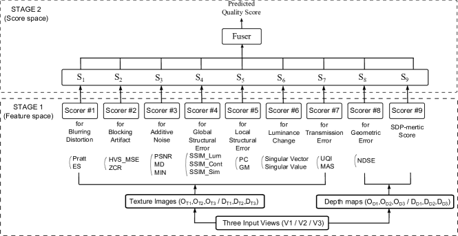
In this work, we adopt the second approach in the design of a SIQA system, which is built upon the parallel boosting (ParaBoost) idea. The proposed PBSIQA system consists of two stages. At Stage I, multiple learning-based scorers are designed, where each scorer handles a specific type of distortion such as the blocking artifact, blurring distortion, additive noise, and so on. The output of these scorers are a normilized objective score that has a value between 0 and 1. The output of these scorers is an obejctive score that only considers the target distortion. At Stage II, the fuser takes scores from all individual scorers to yield the final quality score. The prediction model in the fuser is also obtained from a learning process. The availability of multiple scorers at Stage I enables us to handle complex factors that influence human perceptual quality systematically. In particular, we will investigate the impacts of various distortions in texture and depth maps on the quality of rendered images and, then, take them into account in the design of participating scorers. The design of the PBSIQA system will be detailed in Section V.
Furthermore, we will show the superiority and the robustness of the proposed PBSIQA system by extensive experimental results over several databases consisting of the 2D-plus-depth format as well as the traditional stereoscopic format with symmetric and asymmetric distortions in Section VI. Along this line, we compare the performance of the proposed PBSIQA system against 17 other 2D/3D quality indices.
IV MCL-3D, IVC-A and LIVE-A Databases









The 2D-plus-depth format is adopted in the 3DVC standard due to its several advantages. For example, it allows the texture image and its corresponding depth map image at a few sampled viewpoints to be compressed and transmitted in a visual communication system. After decoding them at a receiver side, we can render several intermediate views between any two input views using depth image based rendering (DIBR) technique. However, very few 3D image quality database was built based on the 2D-plus-depth format. This is one of the main motivations in constructing the MCL-3D database [31]. The MCL-3D database is designed to investigate the impact of texture and/or depth map distortions on the perceived quality of the rendered image so as to develop a robust stereoscopic image quality metric. First, we carefully chose nine texture images and their associated depth maps from a set of 3DVC test seqeunces as references.
To capture the content variety, the Spatial Information (SI) defined by ITU-T recommendation [26] for each texture image and its depth map was calculated. Also, images were carefully extracted from an interval with slow motion to avoid motion blur. This reference set contains indoor/outdoor scenes, CG images, different depth perception, and so on. In Fig. 1, only texture images are shown. Fig. 2 shows the distortion design. There are three original views and each view consists of a texture image and its associated depth map (denoted by /, /, and /). Distortions with different types and levels were applied to original images and/or depth maps. Then, distorted texture images and depth maps were input to the view synthesis reference software (VSRS 3.5 [27]) along with the configuration file provided by the production group to render two intermediate views, and that an assessor will view in the subjective test. We applied six different distortions with four different levels to three input views symmetrically: Guassian blur, sampling blur, JPEG compression, JPEG-2000 compression, additive noise, and transmission error. Based on the recommendations of ITU [28], we consider five quality levels in subjective tests. The original reference stereoscopic images have excellent quality while the other 4-level distorted images were controlled by parameters associated with different distortion types.
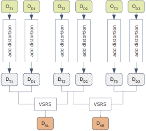
The MCL-3D database consists of the following three sub-databases.
-
•
Dataset A contains texture distortions only.
-
•
Dataset B contains depth map distortions only.
-
•
Dataset C contains both texture and depth map distortions.
The above design allows us to investigate the effect of texture distortions and depth map distortions independently. The test was performed in a controlled environment as recommended by ITU [28], including the display equipment, viewing distance, ambient light, etc. We performed pre-screening of subjects and conducted a training session before the actual test. The subjective test results were verified by a screening process according to Annex 2 of Recommendation BT.500 [29], and outliers were removed. A pairwise comparison was adopted and the comparison result was converted to the mean opinion score (MOS). The MCL-3D database can be downloaded from [31]. For further details, we refer to [30].
In our earlier work [21], we also constructed two new databases by expanding the IVC [32] and the LIVE [33] databases and call them IVC-A and LIVE-A, respectively. We took 12 stereoscopic image pairs from IVC and LIVE as references. While the distortions in IVC and LIVE are symmetric, we add asymmetric distortions in IVC-A and LIVE-A. That is, we add distortions of different levels but the same type to the left and right views of a stereo image pair. There are four distortion types. Each stereoscopic image pair has six combinations of distortion levels: three symmetric distortion levels () and three asymmetric distortion levels (). We conducted a subjective test to obtain MOS using the absolute category rating (ACR) [28]. A summary of the three SIQA databases used in our test is given in Table I.
V Proposed PBSIQA System
| MCL-3D | IVC-A | LIVE-A | ||
|---|---|---|---|---|
| Distortion | Reference Source | Nine texture/depth map images from 3DVC test sequences | Six stereoscopic image pairs from IVC [32] database | Six stereoscopic image pairs from LIVE [33] database |
| # of test images | 648 | 144 | ||
| Distortion type | 6 (gaussian blur / sampling blur / JPEG compression / JPEG2000 compression / additive noise / transmission error) | 4 (gaussian blur / JPEG compression / JPEG2000 compression / additive noise) | ||
| Distortion level | 4 | 4 | ||
| Data format | MVD (Multi-View plus Depthmaps) | Conventional stereoscopic image (only texure image) | ||
| Distortion design | Whole dataset can be divided into three sub-databases. - Dataset A: Distortions only in texture images - Dataset B: Distortions only in depth map images - Dataset C: The same distortion in both texture & depth map images | Each test stereoscopic pair has six combinations of distortion per each distortion type as follows: -[1,1], [1,2], [1,3], [2,2], [2,3] and [3,3] where [l, r] denotes the distortion levels of left and right images & [1]: the strongest, [2]: moderate, and [3]: the weakest distortion. | ||
| Remark | Rendering distortion (two intermediate views are rendered via VSRS3.5) | Contain both symmetric and asymmetric distortions | ||
| Subjective Test | methodology | Pair-wise comparison | ACR-HR (w/ 5 grading scales [1:Bad 5:Excellent]) | |
| participant | 270 people (men: 170, women:100 / ages: 21 - 42) | 20 people (men:19, women:1 / ages: 24 - 37) | ||
| Score type | MOS | MOS | ||
The impact of texture distortions and depth map distortions on rendering quality is different through a view synthesis process. In this section, we first design scorers tailored to texture distortions and depth map distortions in Sec. V-A and Sec. V-B, respectively. The design of these scorers and the score fuser is implemented by support vector regression (SVR) as detailed in Sec. V-C. Finally, the training and test procedures are described in Sec. V-D.
V-A Scorer Design for Texture Distortions
| Type | Feature | Ref | Type | Feature | Ref |
|---|---|---|---|---|---|
| Pixel difference | MD (Maximum Difference) | [35] | Structural Similarity | SSIM index | [36] |
| MAE (Mean Absolute Error) | [37] | SSIM Luminance | [36] | ||
| PSNR | - | SSIM Contrast | [36] | ||
| ABV (Average Block Variance) | - | SSIM Similarity | [36] | ||
| MIN (Modified Infinity Norm) | [37] | UQI (Universal Quality Index) | [40] | ||
| Blockiness | - | SVD related | Singular Value | [39] | |
| AADBIIS (Average Absolute Difference Between In-Block Samples) | [10] | Singular Vector | [39] | ||
| Edge related | ES (Edge Stability) | [37] | Spectral Difference | ZCR (Zero Crossing Rate) | [10] |
| AES (Average Edge Stability) | [10] | PC (Phase Congruency) | [38] | ||
| PRATT | [37] | Contrast measure | GM (Gradient Magnitude) | [38] | |
| Image Correlation | MAS (Mean Angle Similarity) | [37] | HVS | HVS-MSE | [34] |
| NCC (Normalized Cross Correlation) | [37] | View synthesis | NDSE (Noticeable Depth Synthesis Error) | [43] |
In Dataset A of the MCL-3D database, distortions are applied to the texture image while the depth map is kept untouched. In this case, we see a similar distortion in the rendered stereo image. For example, if the texture image is distorted by a transmission error, a similar distortion type is observed in the rendered view since pixel values of the input texture image are direct sources to the pixel intensity of the rendered view.
Furthermore, it is reported in [21] that the interaction between left and right views in perceived 3D image quality depends on the distortion type. For example, for blurring and JPEG-2000 coding distortions, the lost information of a low quality view tends to be compensated by a high quality view. Thus, the perceptual quality is closer to that of the high quality view. On the other hand, for additive noise and JPEG coding distortions, a high quality view is negatively influenced by a low quality view. For this reason, distortions should be carefully classified. We classify distortion types into multiple groups, and design good scorers for them. For each scorer at Stage I, proper features are extracted from input texture images and trained by a learning algorithm. Then, the scorer outputs an intermediate score for the target distortion group.
Based on previous studies on image quality assessment [34, 35, 37, 38, 39, 40] and our own experience, we select 24 candidate features for further examination as listed in Table II. Then, we calculated the Pearson correlation coefficient (PCC) to indicate the prediction performance between MOS and a single-feature-based quality scorer (with the exception that the singular value and the singular vector are integrated into one feature vector for the SVD scorer) over Datasets A and B, respectively. The PCC results of the 23 single-feature-based scorers are shown in one row of Table III. Based on these results, we exclude five features (namely, NCC, AADBIIS, ABV, AES, and blockiness) whose corresponding scorers have low PCC values for Datasets A and B. For the remaining ones, we investigate which features are suitable for which distortion type. For instance, ES and Pratt are useful features to be included in the learning-based scorer targeting at the blurring distortion. In a similar way, we assign candidate features to several scorers as described below.
| PCC | |||||
|---|---|---|---|---|---|
| Feature | Dataset A | Dataset B | Feature | Dataset A | Dataset B |
| ES | 0.83 | 0.44 | HVS_MSE | 0.60 | 0.36 |
| MAS | 0.60 | 0.15 | MAE | 0.68 | 0.63 |
| MD | 0.73 | 0.63 | MIN | 0.70 | 0.63 |
| NCC | 0.34 | 0.16 | PC | 0.78 | 0.32 |
| SMPE | 0.60 | 0.72 | PRATT | 0.78 | 0.56 |
| SSIM index | 0.64 | 0.67 | PSNR | 0.77 | 0.70 |
| UQI | 0.68 | 0.45 | SSIM_CON | 0.68 | 0.68 |
| AADBIIS | 0.27 | 0.52 | SSIM_LUM | 0.78 | 0.62 |
| ABV | -0.20 | 0.38 | SSIM_SIM | 0.58 | 0.49 |
| AES | 0.33 | 0.48 | ZCR | 0.64 | 0.17 |
| BLKNESS | 0.29 | -0.03 | SVD | 0.78 | N/A |
| GM | 0.78 | 0.69 | |||
Scorer #1 for Blurring Distortion: Blurring distortion is mostly caused by low pass filtering, down-sampling, and compression (e.g. JPEG2000) due to the loss of high frequencies. This kind of distortion is referred to as the information loss distortion (ILD) [20]. The perceptual quality of a blurred stereoscopic image pair is closer to that of the high quality view since the structural component of the high quality view is preserved against blurring of the low quality view. Blurring distortion can be observed around edges most obviously. Human are also sensitive to misalignments between the edges of left and right views. Thus, we use two edge-related features to measure blurriness in an image introduced below.
The first one is the edge stability mean squre error (ESMSE) [37], which characterizes the consistency of edges that are evident across multiple scales between the original and distorted images. To compute ESMSE, we first obtain edge maps with five different standard deviation parameters using the Canny operator. The output at scale m is decided by thresholding as
| (1) |
where is the output of the derivative of the Gaussian operator at the mth scale and the threshold is defined as , where and are the maximum and minimum values of the norm of the gradient output in that band, respectively. An edge stability map is obtained by the longest sequence of edge maps such that
| (2) |
where
| (3) |
The edge stability indices for the original and the distorted images at pixel location are denoted by and , respectively. Then, the ESMSE value is calculated by summing the edge stability indices over all edge pixel positions, , of the edge pixels of the original image as
| (4) |
The other one is Pratt’s measure [37] that considers the accuracy of detected edge locations, missing edges and false alarm edges. The quantity is defined as
| (5) |
where and are the number of the detected and the ground truth
edge points, respectively, and is the distance to the closest edge for
the th detected edge pixel. The ground truth of the edge image
is obtained from the uncompressed image, and the value of control parameter
was set to 0.8 experimentally.
Scorer #2 for Blocking Distortion: Blocking distortion is one of the most common distortions generated by block-based image/video coders, such as JPEG, H.264 and HEVC. When stereoscopic images with blocking distortion are shown, the average quality of both views or that of the lower quality is perceived [7, 21]. The high quality image is negatively influenced by the low quality image since blocking distortion introduces new visual artifacts that do not exist in the pristine original scene. Such artifacts are called the information additive distortion (IAD) [20]. As stated in [10, 34], there are two good features in detecting blockiness. They are the HVS-modified MSE (HVS_MSE) and the zero crossing rate (ZCR). Mathematically, the HVS_MSE [34] is given by
| (6) |
where is the image size, and denote original and distorted images, respectively, is the inverse discrete cosine transform (DCT) of , and where , , is an HVS-based band-pass filter and is the DCT of image . The ZCR along the horizontal direction is given by
| (7) |
and where , . The vertical zero crossing rate, , can be computed similarly. Finally, the overall ZCR is given by
| (8) |
Scorer #3 for Additive Noise: Additive noise is often caused by thermal noise during a scene acquisition process. If either view is distorted by additive noise, the perceived quality is degraded by the low quality image. A pixel-based difference is a good measure for additive noise. We select three such features to characterize additive noise: the peak-signal-to-noise ratio (PSNR), the maximum difference (MD) [35] and the modified infinity norm (MIN) [37]. They are defined as
| (9) |
where ;
| (10) |
and
| (11) |
where denotes the th largest deviation
among all pixels. In this work, we select the top deviations,
which means is one fourth of the total number of pixels.
Scorer #4 for Global Structural Error: We consider structural errors since the HVS is highly sensitive to the structural information of the visual stimuli. Structural errors can be captured by three components of the SSIM index [36], which are luminance, contrast and structural similarities between images and . They are defined as
| (12) | |||||
| (13) | |||||
| (14) |
where , , and denote the mean, the standard
deviation and the covariance, respectively.
Scorer #5 for Local Structural Error: The performance of
an image quality scorer can be improved by applying spatially varying
weights to structural errors. Salient low-level features such as edges
provide important information to scene analysis. Two features were
proposed in [38] at this end: phase congruency (PC) and
gradient magnitude (GM). Physiological studies show that PC provides a
good measure for the significance of a local structure. Readers are
referred to [38] for its detailed definition and
properties. While PC is invariant with respect to image contrast, GM
does take local contrast into account.
Scorer #6 for Object Structure and Luminance Change: We utilize singular vectors and singular values as features. Given an image , we can decompose it into the product of two singular vector matrices and and a diagonal matrix in form of
| (15) |
where and are column vectors, is a
singular value and . It was shown in
[39] that the first several singular vectors offer a
good set to represent the structural information of objects while
subsequent vectors account for finer details. Furthermore, singular
values are related to the luminance changes. They should be considered
since the luminance mismatch between left and right views results in
annoying viewing experience.
Scorer #7 for Transmission Error: Packet loss and bit errors occur during stereo image data transmission. It appreas in form of block errors since most image coding standards adopt the block-based approach. Based on the feature analysis, both the universal quality index (UQI) [40] and the mean angle similarity (MAS) [37] are useful in characterizing transmission error. The UQI is defined as
| (16) |
which is equal to the product of three terms representing the loss of correlation, the luminance distortion, and the contrast distortion between two images and , respectively. MAS is a feature that measures the statistical correlation between pixel vectors of the original and the distorted images since similar colors will result in vectors pointing to the same direction in the color space. The moments of the spectral chromatic vector are used to calculte the correlation as
| (17) |
where and indicate the multispectral pixel vectors at position for original and distorted images, respectively, and is the number of pixels that have a non-zero value for the inner product and the norm of and .
For each scorer, three feature values from three input views, denoted by , , and , are fed into the learning-based scorers. We entrust the task of seeking an optimal relation among these features to a learning algorithm, where the impact of the quality difference between left and right views on the perceptual quality highly depends on the distortion type.
V-B Scorer Design for Depth Distortions
Dataset B of the MCL-3D database contains depth map distortions only. Research on the effect of the depth distortion on rendered stereo image quality has been conducted recently by quite a few researchers, e.g., [41, 42]. Generally speaking, the depth value is inversely proportional to the horizontal disparity of rendered left and right views so that the horizontal disparity distortion appears in form of geometric errors.
Scorer #8 for Geometric (Horizontal Disparity) Error: Zhao et al. [43] proposed a Depth No-Synthesis-Error (D-NOSE) model by exploiting that the depth information is typically stored in 8-bit grayscale format while the disparity range for a visually comfortable stereo pair is often far less than 256 levels. Thus, multiple depth values do correspond to the same integer (or sub-pixel) disparity value in the view synthesis process. In other words, some depth distortion may not trigger geometric changes in the rendered view. Specifically, if a pixel distortion of the depth map falls into the range defined by the D-NOSE profile, it does not affect the rendered image quality in terms of MSE. Being motivated by the D-NOSE model, we define a noticeable depth synthesis error (NDSE) feature for geometric errors as
| (18) |
where and represent the original and the distorted depth maps, respectively, and is a pixel index out of the range of D-NOSE profile which is defined as
| (19) |
and where
| (20) | |||||
| (21) |
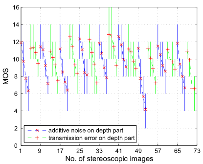
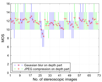
is a quantized depth value, is the disparity function of , is the offset error for the rounding operation, is the precision, and and denote the ceiling and floor operations, respectrively. For more details on the D-NOSE profile, we refer to [43]. Since NDSE only considers pixel distortions that change the original disparity value, it has the highest prediction accuracy (with PCC=0.73) among all features in Table III. However, as compared to those in Dataset A, most features have relatively low PCC values in Dataset B. To investigate further, we divide distorted images into two groups. The first group includes additive noise and transmission errors while the second group includes the Gaussian blur, sampling blur, JPEG compression, and JPEG 2000 compression. For the first group, as the distortion level becomes higher, the MOS decreases monotonically as shown in Fig. 3(a). However, we cannot observe such a coherent MOS movement trend for the second group in Fig. 3(b).
This phenomenon can be explained below. Differences among neighboring
pixels caused by the first group of distortions such as additive noise
or transmission errors are generally large, leading to scattered
geometric distortions in the rendered image especially around object
boundaries. They tend to get worse as the distortion level increases.
On the other hand, differences among neighboring pixels caused by the
second group of distortions are often small and changing gradually.
As a result, we may not be able to recognize them easily although geometric
errors exist in the rendered image.
Scorer #9 - Formula-based Metric:
Due to the weaker correlation between the MOS level and the distortion level as shown in Fig. 3(b), it is diffucult to obtain high prediction accuracy via a learning-based algorithm from features of the input depth map directly. To overcome this challenge, we exploit the auxiliary information from two rendered views. That is, we use the SDP index [21] that is computed based on three depth maps as a candidate scorer. It helps boost the prediction accuracy as presented in Section VI.
V-C Learning-based Scorers and Fuser Design
The proposed PBSIQA system composed by nine quality scorers is summarized in Fig. 4. To yield an intermediate score from scorers #1#8, we adopt the support vector regression (SVR) technique. Consider a set of training data , where is a feature vector and is the target value, e.g. the subjective quality score of the th image. In the -SVR [44], [45], the objective is to find a mapping function that has a deviation at most from the target value, , for all training data. The mapping function is in form of
| (22) |
where is a weighting vector, is a non-linear function, and b is a bias term. We should find and satisfying the following condition:
| (23) |
where is the number of training data.
Although there exist several kernels such as linear, polynomial and sigmoid, we use the radial basis function (RBF) in form of
| (24) |
where is the radius controlling parameter, since it provides good performance in applications [46]. Furthermore, it is not easy to determine a proper value. Thus, we use a different version of the regression algorithm called the -SVR [45], where is a control parameter to adjust the number of support vectors and the accuracy level. In other words, becomes a variable in an optimization problem, and we can obtain the same and more conveniently.
| Scorer # | Target Distortion | AWN sub-database | Gaussian Blur sub-database | JP2K Coding sub-database | JPEG Coding sub-database | Sampling Blur sub-database | Trans. Loss sub-database |
|---|---|---|---|---|---|---|---|
| 1 | Blurring Distortion | 3 (0.80) | 1 (0.89) | 2 (0.84) | 4 (0.77) | 5 (0.70) | 6 (0.57) |
| 2 | Blocking Artifact | 3 (0.81) | 6 (0.67) | 2 (0.82) | 1 (0.88) | 4 (0.80) | 5 (0.70) |
| 3 | Additive Noise | 1 (0.89) | 5 (0.72) | 2 (0.77) | 4 0.75) | 6 (0.66) | 3 (0.76) |
| 4 | Global Structural Error | 1 (0.90) | 4 (0.78) | 3 (0.79) | 2 (0.84) | 6 (0.65) | 5 (0.66) |
| 5 | Local Structural Error | 1 (0.91) | 4 (0.79) | 3 (0.81) | 2 (0.82) | 5 (0.72) | 6 (0.66) |
| 6 | Luminance Change & Scene Structural Error | 4 (0.73) | 5 (0.7) | 2 (0.84) | 1 (0.87) | 3 (0.76) | 6 (0.66) |
| 7 | Transmission Error | 2 (0.82) | 5 (0.64) | 6 (0.63) | 3 (0.68) | 3 (0.68) | 1 (0.84) |
| 8 | Geometric Error | 1 (0.92) | 6 (0.39) | 4 (0.60) | 2 (0.70) | 5 (0.40) | 2 (0.70) |
| Sub-database | Base Performance (#8: Geometric Error) | Blurring Distortion (#2) | Additive Noise (#3) | Blocking Artifact (#1) | Transmission Error (#7) | Structural Error (#4 #5) | Luminance Change (#6) | ||||||
|---|---|---|---|---|---|---|---|---|---|---|---|---|---|
| Perf. Inc. | Perf. Inc. | Perf. Inc. | Perf. Inc. | Perf. Inc. | Perf. Inc. | ||||||||
| AWN | 0.92 | 0.78 | -17.9% | 0.90 | 13.3% | 0.90 | 0.0% | 0.90 | 0.0% | 0.91 | 1.1% | 0.92 | 1.1% |
| Gaussian Blur | 0.35 | 0.86 | 59.3% | 0.89 | 3.4% | 0.93 | 4.3% | 0.93 | 0.0% | 0.94 | 1.1% | 0.95 | 1.1% |
| JP2K | 0.53 | 0.78 | 32.1% | 0.87 | 10.3% | 0.92 | 5.4% | 0.92 | 0.0% | 0.93 | 1.1% | 0.95 | 2.1% |
| JPEG | 0.81 | 0.79 | -2.5% | 0.83 | 4.8% | 0.93 | 10.8% | 0.94 | 1.1% | 0.95 | 1.1% | 0.97 | 2.1% |
| Sampling Blur | 0.45 | 0.84 | 46.4% | 0.78 | -7.7% | 0.87 | 10.3% | 0.90 | 3.3% | 0.91 | 1.1% | 0.93 | 2.2% |
| Trans. Loss | 0.66 | 0.84 | 21.4% | 0.79 | -6.3% | 0.72 | -9.7% | 0.83 | 13.3% | 0.87 | 4.6% | 0.91 | 4.4% |
| Whole Dataset C | 0.58 | 0.74 | 21.6% | 0.84 | 11.9% | 0.89 | 5.6% | 0.91 | 2.2% | 0.92 | 1.1% | 0.93 | 1.1% |
At Stage II of the PBSIQA system, we fuse all intermediate scores from the scorers at Stage I to determine the final quality score. We adopt the -SVR algorithm to implement the fuser. Suppose that there are scorers with training stereoscopic image pairs. For the th training pair, we compute the intermediate quality score , where is the stereoscopic image pair index and is the scorer index. Let be the intermediate score vector for the th image pair. We train the fuser using with all image pairs in the training set and determine the weighting vector and the bias parameter accordingly. Finally, the PBSIQA-predicted quality metric for a given stereoscopic image pair in the test set can be found via
| (25) |
V-D Training and Test Procedures
The -fold cross validation [47] is a common strategy to evaluate the performance of a learning-based algorithm to ensure reliable results and prevent over-fitting, where the data are split into chunks, and one chunk is used as the test data while the remaining chunks are used as training data. We ensured that the model is dominantly trained by the different distortion types from that of testing data since it may boost the prediction accuracy. The same experiment is repeated times by employing each of the chunks as the test data. Finally, the overall performance is determined over all the predicted scores. In the proposed framework, training data are used to generate a regression model of each scorer at Stage I. Then, a regression model of the fuser is obtained by training all intermediate scores from Stage I as input features with -fold cross validation at Stage II, where the number of samples is the same as the number of stereoscopic image pairs in the chunks. In all reported experiment results, we use the 10-fold cross validation. In addition, a feature scaling operation is performed before the training and test processes. It is conducted to avoid features of a larger numeric range dominating those of a smaller numeric range. For example, the PSNR value has a larger range of values than the other two features in scorer #3. We scale the feature values of each scorer to the unit range of [0,1] at Stage I.
At the training stage, our goal is to determine the optimal weighting vector and bias that minimize the error between MOS and the predicted score, i.e.,
| (26) |
Since we use RBF as a kernel function, two parameters and should be optimized to achieve the best regression accuracy. We conduct parameter search on and at the training stage using the cross validation scheme in [46]. Various pairs of are tried, and the one with the best cross validation accuracy is selected. After the best pair is found, the whole training set is used again to generate the final scorer.
At the test stage, we use the intermediate score vector in Eq. (25) to determine the quality score. The test can be quickly done since all model parameters are decided at the training stage.
VI Performance Evaluation
To evaluate the performance of the proposed PBSIQA metric, we follow the suggestions of ITU-T(P.1401) [48] and use three performance measures: 1) the Pearson correlation coefficient (PCC) to measure the linear relationship between a model’s performance and the subjective data , 2) the Spearman rank-order correlation coefficient (SROCC) for the prediction monotonicity, and 3) the root mean squared error (RMSE) for the prediction accuracy. Before calculating the performance measures, we apply the monotonic logistic function to the predicted quality scores so as to fit the subjective quality scores (MOS) and remove any nonlinearity via
| (27) |
where and are the predicted score and the fit predicted score, respectively, and () are the parameters to minimize the mean squared error between and MOS. In addition, this mapping function compensates for offsets, different biases, and other shifts between the scores, without changing the rank order.
VI-A Performance Comparison of Stage I Scorers
First, we compare the performance of eight learning-based scorers (Scorers #1-8) and show that each scorer truly offer good performance for its target distortion type. Here, we consider Datset C of the MLC-3D database only, and divide it into six sub-databases so that each contains one distortion type as described in Section IV. The six distortion types are listed in the top row of Table IV. We compute the PCC value of each scorer against each sub-database and rank its effectiveness in the descending order of PCC values individually. Table IV summarizes the results of scorers in Stage I only (namely, without fusion in Stage II). The performance of scorers #1, #2, and #3 matches well with their target design. First, scorer #1 has the highest correlation on the blurred and JPEG2000 compression sub-databases. This is reasonable since, besides the ringing artifect, the main distortion of the JPEG2000 compression sub-database is blurring. Scorer #2 is designed for the blocking artifact, and the JPEG compression database has the top rank. Scorer #3 has the best performance on additive noise database as designed.
Scorer #4 (for global structural error) and scorer #5 (for local structural error) share strong similarity in their rank orders. Specifically, they provide the first and second best performance in additive noise and JPEG compressed databases. As observed in [21], the information additive distortion (IAD) is more obvious than the information loss distortion (ILD) among all structural distortions. Additive noise and blockiness are typical exmaples of IAD. Our observation is consistent with that in [21]. Scorer #6 yields the best result for the JPEG compressed sub-database since we may see color/luminance chages if the compression ratio is too high, which can be captured by the singular value feature of Scorer #6. However, it has poor correlation with human subjective experience on the additive noise sub-database. This implies that, although scorers #4, #5 and #6 are designed for structural errors in common, they capture different aspects.
Scorer #7 offers the best result for transmission errors to meet the target design. Last, scorer #8, designed to capture geometric distortions, provides the best result in databases with additve noise and transmission errors, which was already explained in Section V-B.
| Dataset A | Dataset B | Dataset C | ||||||||
| Quality Indices | PCC | SROCC | RMSE | PCC | SROCC | RMSE | PCC | SROCC | RMSE | |
| Proposed PBSIQA | 0.921 | 0.913 | 0.703 | 0.848 | 0.775 | 0.580 | 0.933 | 0.920 | 0.741 | |
| 3D indices | BQPNR | 0.591 | 0.533 | 2.241 | 0.675 | 0.512 | 1.181 | 0.617 | 0.522 | 2.339 |
| CYCLOP | 0.742 | 0.730 | 1.758 | 0.805 | 0.730 | 0.981 | 0.791 | 0.772 | 1.513 | |
| RKS | 0.710 | 0.679 | 1.578 | 0.829 | 0.748 | 0.894 | 0.731 | 0.731 | 1.594 | |
| Benoit | 0.560 | 0.559 | 1.855 | 0.698 | 0.533 | 1.147 | 0.593 | 0.593 | 1.884 | |
| Campisi | 0.752 | 0.755 | 1.422 | 0.815 | 0.676 | 0.926 | 0.824 | 0.824 | 1.323 | |
| 2D indices | C4 | 0.788 | 0.796 | 1.402 | 0.818 | 0.676 | 0.921 | 0.824 | 0.833 | 1.323 |
| IFC | 0.639 | 0.593 | 1.722 | 0.662 | 0.160 | 0.199 | 0.671 | 0.609 | 1.733 | |
| MSE | 0.673 | 0.675 | 1.657 | 0.785 | 0.739 | 0.991 | 0.709 | 0.703 | 1.648 | |
| NQM | 0.754 | 0.787 | 1.470 | 0.766 | 0.672 | 1.030 | 0.836 | 0.836 | 1.282 | |
| PSNR_HVS | 0.749 | 0.795 | 1.484 | 0.811 | 0.753 | 0.936 | 0.815 | 0.807 | 1.354 | |
| PSNR | 0.720 | 0.678 | 1.555 | 0.798 | 0.737 | 0.965 | 0.725 | 0.705 | 1.609 | |
| SNR | 0.705 | 0.699 | 1.589 | 0.806 | 0.738 | 0.947 | 0.743 | 0.721 | 1.566 | |
| SSIM | 0.533 | 0.534 | 1.896 | 0.785 | 0.728 | 0.992 | 0.575 | 0.587 | 1.914 | |
| UQI | 0.475 | 0.502 | 1.971 | 0.769 | 0.659 | 1.022 | 0.548 | 0.545 | 1.956 | |
| VIF | 0.663 | 0.656 | 1.677 | 0.746 | 0.582 | 1.066 | 0.696 | 0.671 | 1.678 | |
| VIFP | 0.604 | 0.622 | 1.784 | 0.743 | 0.602 | 1.072 | 0.665 | 0.646 | 1.744 | |
| VSNR | 0.693 | 0.720 | 1.615 | 0.790 | 0.730 | 0.981 | 0.760 | 0.756 | 1.519 | |
VI-B Performance Improvement via Fusion
We show how the PBSIQA system can improve QA performance by fusing the results from scorers at Stage I progressively in this section. To illustrate the design methodology, without loss of generality, we use the performance of scorer #8 for the geometric error as the base, add one scorer at a time to account for the most challenging distortion type in the remaining set, and show how the added scorer improves the performance for six sub-databases and the entire MCL-3D database. The results conducted against Dataset C of the MCL-3D database are shown in Table V, where the base performance with scorer #8 is shown in the first column and the results from scorers #2, #3, #1, #7, #4, #5, and #6 are fused to its score one by one cumulatively. We see a substantial performance gain for each sub-database when its associated scorer is included in the fusion process. The whole database contains different distortion types so that it is beneficial to fuse all scorers to get robust and accurate predicted quality scores as shown in the last row of Table V. The design methodology (namely, the fusion order of scorers #2, #3, #1, #7, #4 and #5 and, finally, #6) is explained below. The performance gain for a given database is calculated in percentages as
| (28) |
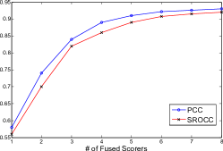
where is the value of PCC after adding a new scorer, while is the result of the previous stage. Since the error rate of base scorer #8 is highest in sub-databases with Gaussian/sampling blur, we fuse scorer #2 to scorer #8 to reduce erroneous prediction caused by blurring distortion. We show the performance improvement for each sub-database in the second column of Table V and see about 60% and 45% performance gains for sub-databases with the Gaussian and the sampling blur, respectively. Although the performance gain drops in some sub-databases, they are not as significant. As a result, we achieve a performance gain of 21.6% for the entire database. After the fusion of scorers #8 and #2, it is shown in Table V that the system does not perform well against additive noise. Thus, we fuse scorer #3 to the system in the next step. After the fusion of scorers #8, #2 and #3, we observe a significant performance boost (13%) for the additive noise sub-database, and a performance gain of 11.9% for the entire database. By following the same line of thought, we can fuse more scorers and obtain better performance for the entire database. Based on the above discussion, both PCC and SROCC values with respect to the whole MCL-3D database are plotted as a function of the number of fused scorers in Fig. 5. The performance of the proposed PBSIQA system may reach a saturation point if the number of fused scorers is sufficiently larger. It should also be emphasized that the proposed PBSIQA system can be extended systematically. That is, if new distortion types are introduced, we can design scorers to tailor to them and fuse new scorers into the system. In contrast, the traditional formula-based quality metric does not have such flexibility.
VI-C Performance Comparison with Other Quality Indices
In this section, we compare the performance of the proposed PBSIQA metric with other QA metrics against Datasets A, B, and C of MCL-3D, IVC-A and LIVE-A. The latter two are more challenging than their sources, IVC [32] and LIVE [33], by including asymmetric distortions. Futhermore, we conduct a cross-database learning procedure to demonstrate the robustness of the proposed PBSIQA metric. That is, the PBSIQA trained with the MCL-3D database is used to predict the quality of stereo image pairs in IVC-A and LIVE-A. For performance benchmarking, we consider both 3D and 2D quality indices in the literature. The 3D indices include those denoted by Benoit [12], Campisi [11], RKS [20] and BQPNR [23]. The 2D indices include: the Signal to Noise Ratio (SNR), the Peak Signal to Noise Ratio (PSNR), the Mean Square Error (MSE), the Noise Quality Measure [49] (NQM), the Universal Quality Index [40] (UQI), the Structural Similarity Index [36] (SSIM), the pixel-based VIF [50] (VIFP), the visual signal-to-noise ratio [51] (VSNR), the Peak Signal to Noise Ratio taking into account CSF [52] (PSNR-HVS), C4 [53], and the image fidelity criterion [54] (IFC). Since 2D metrics are only applied to a single image, we use the average score of left and right rendered views to yield the overall quality metric. We first focus on performance comparison against the MCL-3D database. The results are summarized in Table VI, where the best and second best metrics in each column of are shown in bold. We have the following observations.
-
•
Dataset A of MCL-3D (texture distortion only)
The PBSIQA system has the best performance in terms of PCC, SROCC and RMSE. It outperforms all other 2D and 3D indices by a significant margin. Among the 2D indices, those designed by considering HVS offer better performance such as C4, NQM, and PSNR_HVS. -
•
Dataset B of MCL-3D (depth map distortion only)
The PBSIQA system gives the best performance in PCC, SROCC and RMSE, yet its performance gain over the second best one narrows. Note that there are only two scorers (scorers #8 and #9) in the PBSIQA system dedicated to the depth map distortion. -
•
Dataset C of MCL-3D (both texture and depth map distortions)
The PCC and the SROCC values of the PBSIQA metric are 0.933 and 0.920, respectively. It outperforms all benchmarking indices by a significant margin.
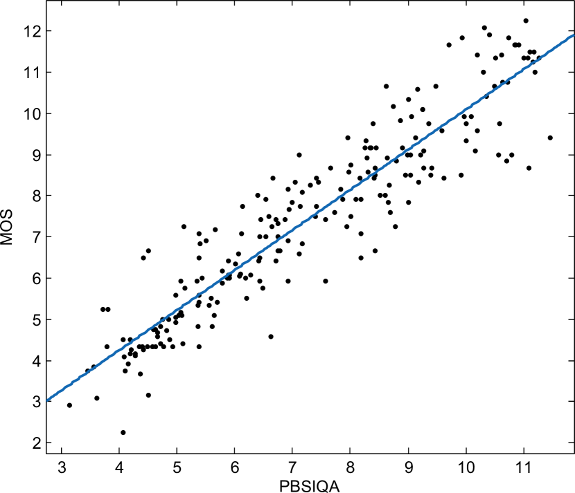
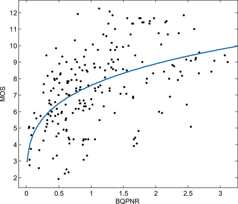
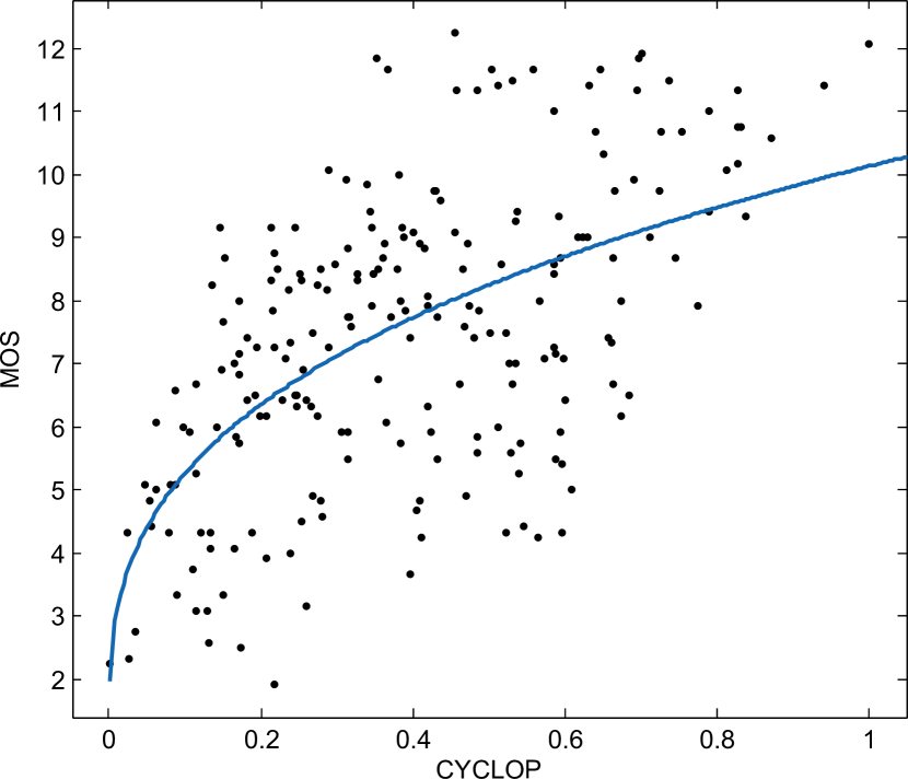
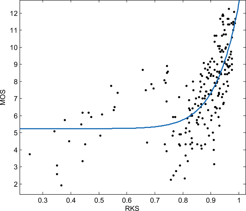
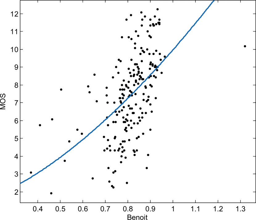
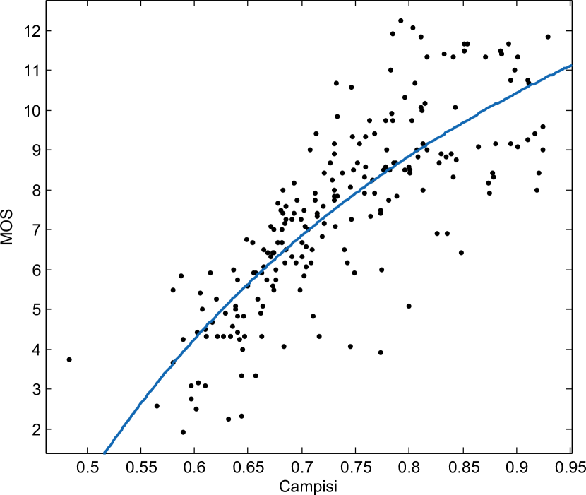
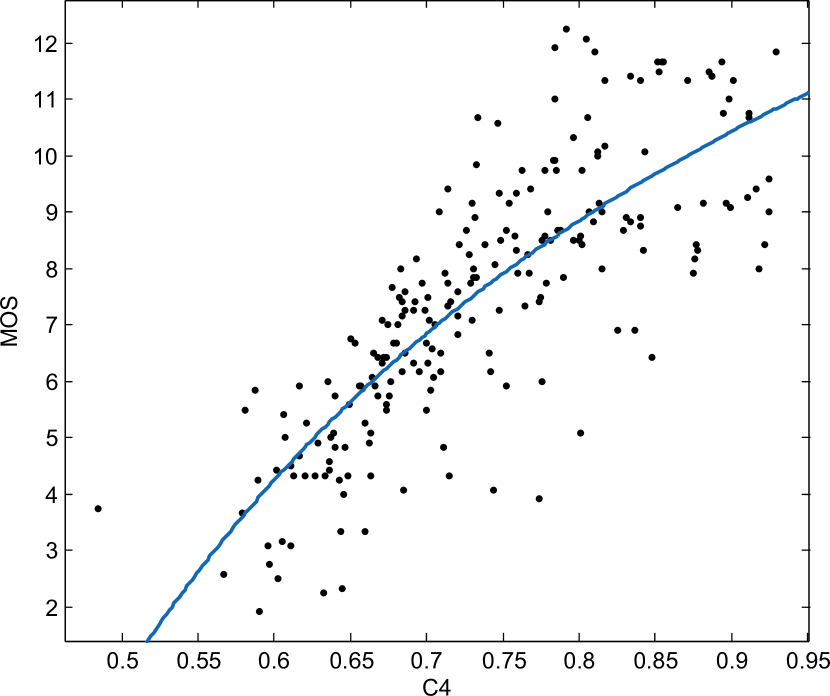
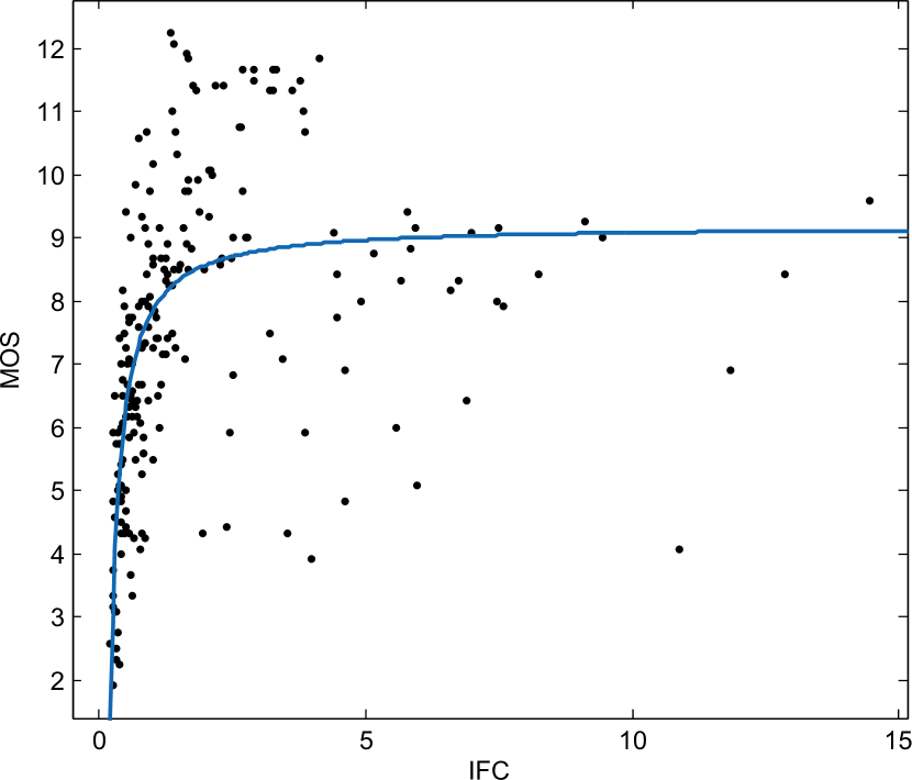
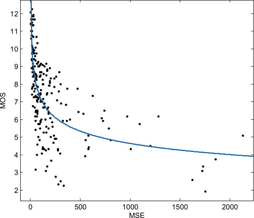
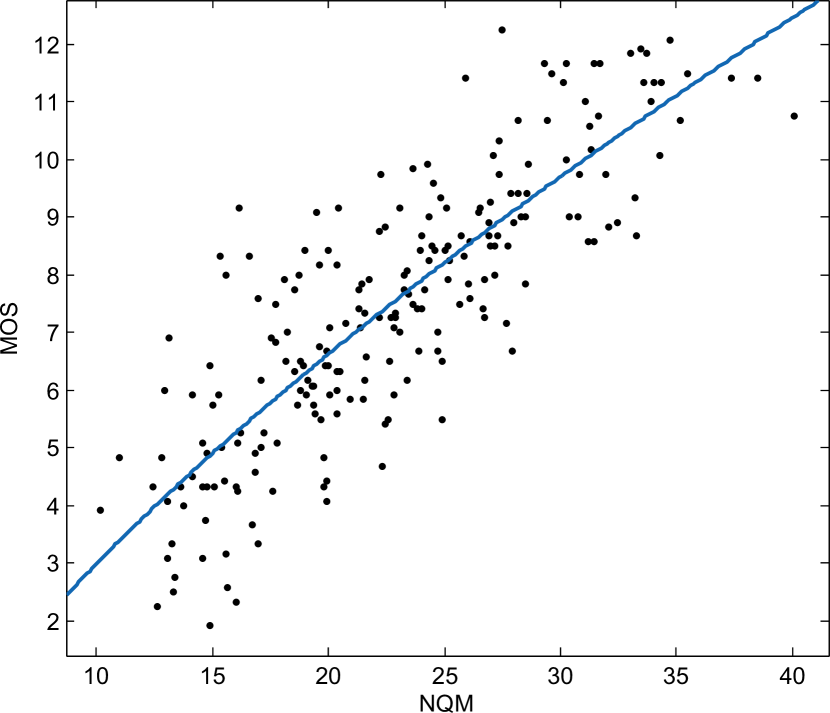
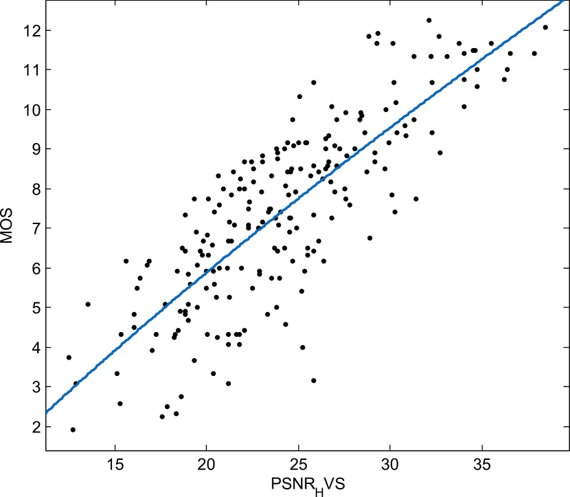
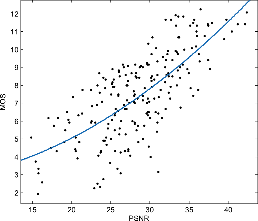
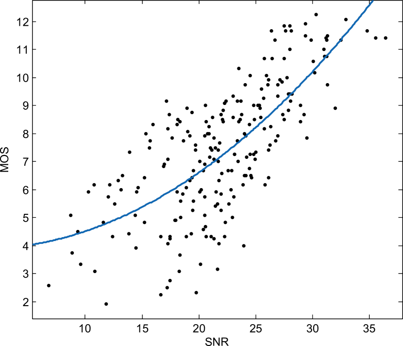
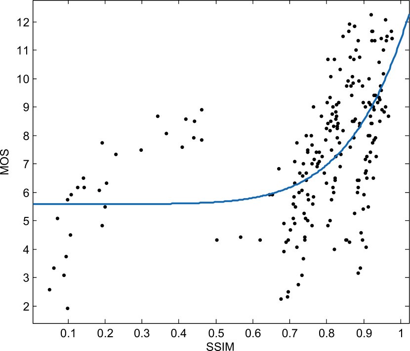
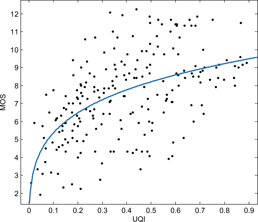
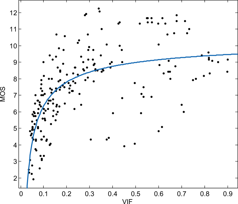
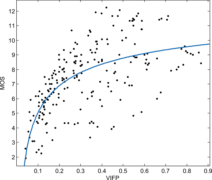
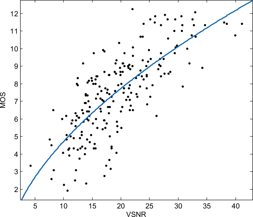
The scatter plots of predicted scores vs. MOS along with their fitting curves approximated by function with 95% confidence level for 18 objective quality metrics are shown in Fig. 6. These data are calculated based on Dataset C of MCL-3D. Each point on the plot represents one stereoscopic image pair. The horizontal axis gives the objective quality score while the vertical axis indicates the MOS value. The scatter plots confirm that the PBSIQA metric exhibits the best correlation with human perception. On the other hand, many of existing algorithms such as IFC, SSIM, UQI lose the monotonic property with respect to MOS as demonstrated in SROCC values of Table VI. Although the fitting curves of NQM and PSNR_HVS show trends similar to that PBSIQA, their variances are much larger.
| PCC | ||||
|---|---|---|---|---|
| Rank | IVC-A Database | LIVE-A Database | ||
| 1 | PBSIQA | 0.952 | PBSIQA | 0.924 |
| 2 | RKS | 0.884 | RKS | 0.841 |
| 3 | SSIM | 0.821 | SSIM | 0.841 |
| 4 | C4 | 0.811 | Campisi | 0.781 |
| 5 | Campisi | 0.746 | C4 | 0.776 |
| 6 | CYCLOP | 0.711 | PSNR | 0.733 |
| 7 | PSNR | 0.671 | VIFP | 0.654 |
| 8 | BQPNR | 0.614 | VSNR | 0.654 |
| 9 | UQI | 0.591 | CYCLOP | 0.652 |
| 10 | Benoit | 0.569 | VIF | 0.642 |
| 11 | VIF | 0.568 | BQPNR | 0.633 |
| 12 | NQM | 0.555 | UQI | 0.631 |
| 13 | VIFP | 0.545 | PSNR_HVS | 0.612 |
| 14 | SNR | 0.544 | Benoit | 0.607 |
| 15 | IFC | 0.532 | SNR | 0.598 |
| 16 | PSNR_HVS | 0.531 | NQM | 0.558 |
| 17 | MSE | 0.523 | MSE | 0.546 |
| 18 | VSNR | 0.407 | IFC | 0.524 |
| Database | PCC | SROCC | RMSE |
|---|---|---|---|
| IVC-A | 0.884 | 0.853 | 0.404 |
| LIVE-A | 0.893 | 0.844 | 0.433 |
Next, we show the performance comparison over IVC-A and LIVE-A databases in Table VII. We only fuse scorers #1#7 for texture distortions in the PBSIQA system since these two databases consist of the stereoscopic data format (i.e., the left and the right views without the depth map). As shown in Table VII, PBSIQA still outperforms existing metrics significantly. For example, the PCC values of PBSIQA for IVC-A and LIVE-A are 0.952 and 0.924, respectively while those of the second best metric (RSK) are 0.884 and 0.841. We see that the PCC values of PBSIQA for these two databases are higher than that for MCL-3D. This is due to the fact that the distortion types in IVC-A and LIVE-A are simpler than that of MCL-3D so that each scorer can generate more reliable scores for them.
Practically, it is not convenient to train learning-based quality assessment indices to tailor to a new database every time. It is desirable to develop a quality metric that offers consistent performance when it is trained by one database yet tested by a different database. This is called cross-database validation. To conduct this task, we train the PBSIQA system using the MCL-3D database and then use it to predict the quality score of stereoscopic images in IVC-A and LIVE-A. The results are shown in Table VIII. Although its performance degrades slightly, the PBSIQA system still offers good results. As the SIQA database size becomes larger, its prediction accuracy goes higher. Finally, it is worthwhile to point out that, since the PBSIQA system consists of multiple individual scorers, its complexity is roughly equal to the total complexity of all contributing scorers. Basically, it trades higher complexity for better performance.
VII Conclusion and Future work
In this work, we proposed a ParaBoost method to design a new stereoscopic image quality assessment system called PBSIQA, which includes a set of parallel quality scorers designed to address various distortions in Stage I and their scores are fused to yield the ultimate quality score in Stage II. The excellent performance of the PBSIQA system was collaborated by extensive experimental results. Our research has an impact to the 3D content delivery field since a reliable 3D quality assessment metric serves as a valuable objective function in optimizing the overall system performance.
As future extensions, it is interesting to incorporate the masking effect. For example, distortions in salient regions such as foreground objects have more negative impacts on perceptual quality. Also, textured regions are usually more robust to distortions, whereas distortions in homogeneous regions are more noticeable. We may further improve performance by considering content characteristics.
Another interesting extension is to consider the quality assessment of 3D video. On one hand, we believe that the ParaBoost methodology can be extended to the case of 3D video in principle. On the other hand, we do need sufficiently large 3D video quality assessment databases for the learning-based methodology to apply. The lack of publicly accessible 3D video quality assessment databases is the main barrier to this research and it is desired to develop such databases for the research community.
Acknowledgment
Computation for the work described in this paper was supported by the University of Southern California’s Center for High-Performance Computing (hpc.usc.edu).
References
- [1] ISO/IEC JTC1/SC29/WG11, “Text of ISO/IEC FDIS 23000-11 for Stereoscopic Video AF,” N10283, Busan, Korea, Oct. 2008.
- [2] A. Vetro, T. Wiegand, and G. J. Sullivan, “Overview of the Stereo and Multiview Video Coding Extensions of the H.264/ MPEG-4 AVC Standard,” in Proc. of the IEEE, vol. 99, no. 4, pp. 626-642, Apr. 2011.
- [3] K. Muller, P. Merkle, and T. Wiegand,“3-D Video Representation Using DepthMaps,” in Proc. of the IEEE, vol. 99, no. 4, pp. 643-656, Apr. 2011.
- [4] L. Yu-Hsun and JL. Wu, “Quality assessment of stereoscopic 3D image compression by binocular integration behaviors,” IEEE Transactions on Image Processing, vol. 23, pp. 1527-1542, Apr. 2014.
- [5] L. B. Stelmach, W. J. Tam, D. V. Meegan, A. Vincent, and P. Corriveau, “Human perception of mismatched stereoscopic 3D inputs”, in Proc. IEEE ICIP, vol. 1, pp. 5-8, 2000.
- [6] D. V. Meegan, L. B. Stelmach, and W. J. Tam, “Unequal weighting of monocular inputs in binocular combination: Implications for the compression of stereoscopic imagery”, Journal of Experimental Psychology: Applied, vol. 7, pp. 143, 2001.
- [7] P. Seuntiens, L. Meesters, and W. Ijsselsteijn, “Perceived quality of compressed stereoscopic images: Effects of symmetric and asymmetric JPEG coding and camera separation,” ACM Transactions on Applied Perception (TAP), vol. 3, pp. 95-109, Apr. 2006.
- [8] P. Kauff, N. Atzpadin, C. Fehn, M. Muller, O. Schreer, A. Smolic, and R. Tanger, “Depth map creation and image based rendering for advanced 3DTV services providing interoperability and scalability,” Signal Process., Image Commun., vol. 22, no. 2, pp. 217-234, Feb. 2007.
- [9] S. Winkler, “Digital video quality: vision models and metrics”, John Wiley & Sons, 2005.
- [10] T.-J. Liu, W. Lin, and C.-C. J. Kuo, “Image quality assessment using multi-method fusion,” IEEE Transactions on Image Processing, vol. 22, no. 5, pp. 1793-1807, May. 2013.
- [11] P. Campisi, P. Le Callet, and E. Marini, “Stereoscopic image quality assessment,” in Proc. 15th European Signal Processing Conference,, Sep. 2007
- [12] A. Benoit, P. Le Callet, P. Campisi, and R. Cousseau, “Using disparity for quality assessment of stereoscopic images,” in Proc. IEEE ICIP, pp. 389-392, Oct. 2008.
- [13] P.Hanhart and T. Ebrahimi, “Quality assessment of a stereo pair formed from decoded and synthesized views using objective metrics,” in Proc. 3DTV-CON, pp. 1-4, Oct. 2012.
- [14] P. Hanhart and T. Ebrahimi, “Quality assessment of a stereo pair formed from two synthesized views using objective metrics,” in 7th VPQM, Jan. 2013.
- [15] Z. M. P. Sazzad, R. Akhter, J. Baltes, and Y. Horita, “Objective No-Reference Stereoscopic Image Quality Prediction Based on 2D Image Features and Relative Disparity,” Advances in Multimedia, vol. 2012, Jan. 2012.
- [16] P. Gorley and N. Holliman, “Stereoscopic Image Quality Metrics and Compression,” in International Society for Optics and Photonics Electronic Imaging, pp. 680305-680305, 2008.
- [17] A. Maalouf and M.C. Larabi, “CYCLOP: A stereo color image quality assessment metric,” in IEEE International Conference on Acoustics, Speech and Signal Processing (ICASSP), pp. 1161-1164, May, 2011.
- [18] C.T. Hewage and M. G. Martini, “Reduced-reference quality assessment for 3D video compression and transmission,” IEEE Transactions on Consumer Electronics, vol. 57, no. 3, pp. 1185-1193, 2011.
- [19] T. Kim, J. Kang, S. Lee, and A. Bovik, “Multimodal interactive continuous scoring of subjective 3D video quality of experience,” IEEE Transactions on Multimedia, vol. 16, no. 2, pp. 387-402, 2014.
- [20] S. Ryu, D. Kim, and K. Sohn, “Stereoscopic image quality metric based on binocular perception model,” in Proc. IEEE ICIP, vol. 1, pp. 609-612, Sep. 2012.
- [21] H. Ko, C. Kim, S. Choi, and C.-C. J. Kuo, “3D image quality index using SDP-based binocular perception model,” in IEEE 11th IVMSP Workshop, pp. 1-4, Jun. 2013.
- [22] F. Shao, L. Weisi, G. Shanbo, J. Gangyi, and S. Thambipillai, “Perceptual full-reference quality assessment of stereoscopic images by considering binocular visual characteristics,” IEEE Transactions on Image Processing, vol. 22, no. 5, pp. 1940-1953, May, 2013.
- [23] S. Ryu, and K. Sohn, “No-Reference Quality Assessment for Stereoscopic Images Based on Binocular Quality Perception,” IEEE Transactions on Circuits and Systems for Video Technology, vol. 24, no. 4, pp. 591-602, Apr, 2014.
- [24] M. Park, L. Jiebo, and C. G. Andrew, “Toward Assessing and Improving the Quality of Stereo Images,” IEEE Journal of Selected Topics in Signal Processing,, vol. 6, no. 5, pp. 460-470, 2012.
- [25] J. Cheng and L. Sumei, “Objective Quality Assessment of Stereo Images Based on ICA and BT-SVM,” in IEEE 7th International Conference on Computer Science & Education (ICCSE), pp. 154-159, 2012.
- [26] ITU, “Recommendation ITU-T P.910, Subjective video quality assessment methods for multimedia applications,” tech. rep., ITU-T, Geneva, 1996.
- [27] View Synthesis Reference Software (VSRS 3.5) [Online]. Available: http://wg11.sc29.org/svn/repos/MPEG-4/test/tags/3D/view−synthesis /VSRS−3−5
- [28] ITU-R, “Recommendation ITU-R BT.2021: Subjective methods for the assessment of stereoscopic 3DTV systems,” in tehc.rep., 2012.
- [29] ITU-R, “BT.500-11: Methodology for the subjective assessment of the quality of television pictures,” in tech. rep., 2002.
- [30] R. Song, H. Ko, and C.-C. J. Kuo, “MCL-3D: a database for stereoscopic image quality assessment using 2D-image-plus-depth source,” accepted by Journal of Information Science and Engineering.
- [31] MCL-3D database is available online, “http://mcl.usc.edu/mcl-3d-database/”
- [32] A. Benoit, P. L. Callet, P. Campisi, and R. Cousseau, “IRCCyN/IVC 3D images database,” ACM Transactions on Applied Perception (TAP), IVC-Database [Online]. Available: “http://www.irccyn.ec-nantes.fr/spip.php?article876”, 2008
- [33] A. K. Moorthy, C. C. Su, A. Mittal, and A. C. Bovik, “Subjective evaluation of stereoscopic image quality,” Signal Processing: Image Communication, LIVE-Database [Online]. Available: “live.ece.utexas.edu/research/quality/live_3dimage_phase1.html”, 2012.
- [34] T. H. Falk, Y. Guo, and W. Y Chan, “Improving robustness of image quality measurement with degradation classification and machine learning,” in Proc. Conference Record of the Forty-First Asilomar Conference on Signals, Systems and Computers (ACSSC 2007), pp. 503-507, 2007.
- [35] A. M. Eskicioglu and P. S. Fisher, “Image quality measures and their performance,” IEEE Transaction on Communications, vol. 43, pp. 2959–2965, Dec. 1995
- [36] Z. Wang, A.C. Bovik, H.R. Sheikh, and E.P. Simoncelli, “Image quality assessment: From error visibility to structural similarity,” IEEE Transactions on Image Processing, vol. 13, pp. 600-612, Apr. 2004.
- [37] I. Avcibas, B. Sankur, and K. Sayood, “Statistical evaluation of image quality measures,” Journal of Electronic imaging, vol. 11, pp. 206-223, 2002.
- [38] L. Zhang, L. Zhang, X. Mou, and D. Zhang “FSIM: a feature similarity index for image quality assessment,” IEEE Transactions on Image Processing, vol. 20, pp. 2378-2386, Aug. 2011.
- [39] M. Narwaria and W. Lin, “SVD-based quality metric for image and video using machine learning,” IEEE Transactions on Systems, Man, and Cybernetics, Part B: Cybernetics, vol. 42, pp. 347-364, Apr. 2012.
- [40] Z. Wang and A. Bovik, “A Universal Image Quality Index,” IEEE Signal Processing Letter, vol. 9, no 3, Mar. 2002.
- [41] W. S. Kim, A. Ortega, P. L. Lai, D. Tian, and C. Gomila, “Depth map coding with distortion estimation of rendered view,” SPIE Vis. Inf. Process. Commun., 2010.
- [42] B. T. Oh, J. Lee, and D.-S. Park, “Depth map coding based on synthesized view distortion function,” IEEE J. Sel. Topics Signal Process., vol. 5, no. 7, pp. 1344–1352, Nov. 2011.
- [43] Y. Zhao, C. Zhu, Z. Chen, and L. Yu, “Depth no-synthesis-error model for view synthesis in 3-D video,” IEEE Trans. Image Process., vol. 20, no. 8, pp. 2221–2228, Aug. 2011.
- [44] B. Schölkopf, and A. J. Smola “Learning with kernels: support vector machines, regularization, optimization and beyond,” the MIT Press, 2002.
- [45] D. Basak, S. Pal, and D. C. Patranabis “Support vector regression,” Neural Information Processing-Letters and Reviews, vol. 11, no. 10, pp. 203-224, Oct, 2007.
- [46] C.-W. Hsu, C.-C. Chang, and C.-J Lin “A practical guide to support vector classification,” Dept. Comput.Sci., National Taiwan Univ., Taipei, Taiwan, Tech. Rep., Apr. 2010.
- [47] C. M. Bishop, “Pattern recognition and machine learning,” Vol. 1, New York: springer, 2006.
- [48] ITU-T, “P.1401: Statistical analysis, evaluation and reporting guidelines of quality measurements,” in tech. rep., 2012.
- [49] N. Damera-Venkata, T. D. Kite, W. S. Geisler, B. L. Evans, and A.C. Bovik, “Image quality assessment based on a degradation model,” IEEE Transactions on Image Processing, vol. 4, no. 4, pp. 636-650, Apr. 2000.
- [50] H. R. Sheikh, and A. C. Bovik, “Image information and visual quality,” IEEE Transactions on Image Processing, vol. 15, no. 2, pp. 430-444, Feb. 2006.
- [51] D. M. Chandler and S. S. Hemami, “VSNR: A wavelet-based visual signal-to-noise ratio for natural images,” IEEE Transactions on Image Processing, vol. 16, no. 9, pp. 2284-2298, Sep. 2007.
- [52] N. Ponomarenko, F. Silvestri, K. Egiazarian, M. Carli, J. Astola, and V. Lukin, “On between-coefficient contrast masking of dct basis functions,”in Proc. 3rd Int. Workshop Video Process. Quality Metrics Consum. Electron., Scottsdale, AZ, Jan. 2007.
- [53] M. Carnec, P. Le Callet, and D. Barba, “An image quality assessment method based on perception of structural information,” in Proc. IEEE ICIP, vol. 3, pp. III-185, Sep. 2003.
- [54] H. R. Sheikh, A. C. Bovik, and G. De Veciana “An information fidelity criterion for image quality assessment using natural scene statistics,” IEEE Transactions on Image Processing, vol. 14, no. 12, pp. 2117-2128, Dec. 2005.