Robust Uncalibrated Stereo Rectification with Constrained Geometric Distortions (USR-CGD)

Abstract

A novel algorithm for uncalibrated stereo image-pair rectification under the constraint of geometric distortion, called USR-CGD, is presented in this work. Although it is straightforward to define a rectifying transformation (or homography) given the epipolar geometry, many existing algorithms have unwanted geometric distortions as a side effect. To obtain rectified images with reduced geometric distortions while maintaining a small rectification error, we parameterize the homography by considering the influence of various kinds of geometric distortions. Next, we define several geometric measures and incorporate them into a new cost function for parameter optimization. Finally, we propose a constrained adaptive optimization scheme to allow a balanced performance between the rectification error and the geometric error. Extensive experimental results are provided to demonstrate the superb performance of the proposed USR-CGD method, which outperforms existing algorithms by a significant margin.

I Introduction

Stereo vision is used to reconstruct the 3D structure of a real world scene from two images taken from slightly different viewpoints. Recently, stereoscopic visual contents have been vastly used in entertainment, broadcasting, gaming, tele-operation, and so on. The cornerstone of stereo analysis is the solution to the correspondence problem, which is also known as stereo matching. It can be defined as locating a pair of image pixels from left and right images, where two pixels are the projections from the same scene element. A pair of corresponding points should satisfy the so-called epipolar constraint. That is, for a given point in one view, its corresponding point in the other view must lie on the epipolar line. However, in practice, it is difficult to obtain a rectified stereo pair from a stereo rig since it often contains parts of mechanical inaccuracy. Besides, thermal dilation affects the camera extrinsic parameters and some internal parameter. For example, the focal length can be changed during shooting with different zoom levels. For the above-mentioned reasons, epipolar lines are not parallel and not aligned with the coordinate axis and, therefore, we must search through the 2D window, which makes the matching process a time-consuming task.

The correspondence problem can however be simplified and performed efficiently if all epipolar lines in both images are in parallel with the line connecting the centers of the two projected views, which is called the baseline. Since the corresponding points have the same vertical coordinates, the search range is reduced to a 1D scan line. This can be embodied by applying 2D projective transforms, or homographies, to each image. This process is known as “image rectification” and most stereo matching algorithms assume that the left and the right images are perfectly rectified.

If intrinsic/extrinsic camera parameters are known from the calibration process, the rectification process is unique up to trivial transformations. However, such parameters are often not specified and there exists a considerable amount of uncertainty due to faulty calibration. On the other hand, there are more degrees of freedom to estimate the homography of uncalibrated cameras. The way to parameterize and optimize these parameteres is critical to the generation of rectified images without unwanted warping distortions.

As pioneering researchers on image rectification, Ayache and Francis [1] and Fusiello et al. [2] proposed rectification algorithms based on known camera parameters. The necessity of knowing calibration parameters is the major shortcoming of these early methods. To overcome it, several researchers proposed a technique called projective (or uncalibrated) rectification that rectifies images without knowing camera parameters but estimating homography using epipolar geometry under various constraints. Hartley and Andrew [3, 4] developed a theoretical foundation for this technique, where they derived a condition for one of two homographies to be close to a rigid transformation while estimated the other by minimizing the difference between the corresponding points. Loop and Zhang [5] estimated homographies by decomposing them into a projective transform and an affine transform.

There exist rectification algorithms that take geometric distortions into account to prevent them from being introduced in the rectified images. For example, Pollefeys et al. [6] proposed a simple and efficient algorithm for a stereo image pair using a polar parametrization of the image around the epipole while Gluckman and Nayar [7] presented a rectification method to minimize the resampling effect, which corresponds to the loss or creation of pixels due to under- or over-sampling, respectively. A similar approach was developed by Mallon and Whelan in [8], where perspective distortions are reduced by applying the singular vector decomposition (SVD) to the first order approximation of an orthogonal-like transfrom. Isgro and Trucco [9] proposed a new approach to estimate homographies without explicit computation of the fundamental matrix by minimizing the disparity as done in [3]. However, such a constraint on the disparity sometimes generates significantly distorted image. For further improvement, Wu and Yu [10] combined this approach with a shearing transform to reduce the distortion.

More recently, Fusiello and Luca [11] proposed a Quasi-Euclidean epipolar rectification method that approximates the Euclidean (calibrated) case by enforcing the rectifying transformation to be a collineation induced by the plane at the infinity, which does not demand a specific initialization step in the minimization process. Zilly et al. [12] proposed a technique to estimate the fundamental matrix with the appropriate rectification parameter jointly. However, their method is limited to the case with almost parallel stereo rigs and a narrow baseline. Georgiev et al. [13] developed a practical rectification algorithm of lower computational cost, yet it is only applicable in the probable stereo setup.

In this work, we propose a novel rectification algorithm for uncalibrated stereo images, which demands no prior knowledge of camera parameters. Although quite a few methods are proposed to reduce unwanted warping distortions in rectified images with different homography parameterization schemes, there is no clear winner among them. Additionally, only two geometric measures (namely, orthogonality and the aspect-ratio) are used as geometric distortion criteria while they are not sufficient in characterizing the subjective quality of all rectified images. Here, we analyze the effect of various geometric distortions on the quality of rectified images comprehensively, and take them into account in algorithmic design. The proposed USR-CGD algorithm minimizes the rectification error while keeping errors of various geometric distortion types below a certain level.

The main contributions of this work are summarized below.

• An uncalibrated stereo rectification algorithm is proposed to minimize the rectification error with constrained geometric distortions. A variety of geometric distortions such as the aspect-ratio, rotation, skewness and scale-variance are introduced and incorporated in the new cost function, then it is minimized by our novel optimization scheme.

• A parameterization scheme for rectifying transformation is developed. The parameters include the focal length difference between two cameras, the vertical displacement between optical centers, etc. This new scheme helps reduce the rectification error by adding more degrees of freedom to the previous Euclidean model [11].

• We provide a synthetic database that contains six geometric distortion types frequently observed in uncalibrated stereo image pairs. It allows a systematic way to analyze the effect of geometric distortions and parameterize the rectifying transformations accordingly. We also provide a real world stereo database with various indoor and outdoor scenes of full-HD resolution. The performance of several algorithms can be easily evaluated with these two databases.

The rest of this paper is organized as follows. The mathematical background on uncalibrated rectification is reviewed in Section II. The proposed USR-CGD algorithm is elaborated in Section III. Two existing and two new databases for unrectified stereo images are described in Section IV. Experimental results and discussions are provided in Section V. The superiority of the proposed USR-CGD algorithm are demonstrated by extensive experiments in the four above-mentioned databases. Finally, concluding remarks are given in Section VI.

II Uncalibrated Rectification

We briefly review the mathematical background on perspective projection and epipolar geometry for uncalibrated rectification in this section. As shown in Fig. 1, the pinhole camera model consists of optical center $C$, image plane $R$, object point $W$, and image point $M$ that is the intersection of $R$ and the line containing $C$ and $W$. The focal length is the distance between $C$ and $R$, and the optical axis is the line that is orthogonal to $R$ and contains $C$, where its intersection with $R$ is the principal point.

Figure 1: Illustration of a pinhole camera model.

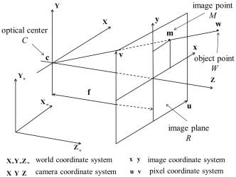
Let $\mathbf{w}$ and $\mathbf{m}$ be the coordinates of $W$ and $M$, respectively. They are related by a perspective projection matrix $\mathbf{P}$ of dimension $3\times 4$ as

$$\mathbf{m}=\left[\begin{array}[]{ccc}u\\ v\\ 1\end{array}\right] \simeq \left[\begin{array}[]{cccc}p_{11}&p_{12}&p_{13}&p_{14}\\ p_{21}&p_{22}&p_{23}&p_{24}\\ p_{31}&p_{32}&p_{33}&p_{34}\end{array}\right]\left[\begin{array}[]{cccc}x\\ y\\ z\\ 1\end{array}\right]$$ (11)

$$= \mathbf{P}\mathbf{w},$$ (12)

where $\simeq$ indicates the equal up to scale. Matrix $\mathbf{P}$ can be decomposed into

$$\mathbf{P}=\mathbf{K}\left[\mathbf{R}\mid\mathbf{t}\right],$$ (13)

where $\mathbf{K}$ and $\left[\mathbf{R}\mid\mathbf{t}\right]$ are called the camera intrinsic matrix and the camera extrinsic matrix, respectively. Matrix $\mathbf{K}$ is in form of

$$\mathbf{K}=\left[\begin{array}[]{ccc}\alpha_{u}&\gamma&u_{0}\\ 0&\alpha_{v}&v_{0}\\ 0&0&1\end{array}\right],$$ (14)

where $\alpha_{u}=s_{u}f$ and $\alpha_{v}=s_{v}f$ are focal lengths in the $u$ and $v$ axes, respectively ($f$ is the physical focal length of the camera in the unit of millimeters while $s_{u}$ and $s_{v}$ are the scale factors), and $(u_{0},v_{0})$ are the coordinates of the principal point, $\gamma$ is the skew factor when the $u$ and the $v$ axes of the model are not orthogonal. For simplicity, it is often assumed that the horizontal and vertical focal lengths are the same and there is no skew between $u$ and $v$ axes. Thus, we have

$$\mathbf{K}=\left[\begin{array}[]{ccc}\alpha&0&\frac{w}{2}\\ 0&\alpha&\frac{h}{2}\\ 0&0&1\end{array}\right],$$ (15)

where $w$ and $h$ are the width and the height of the image, respectively. The camera extrinsic matrix of dimension $3\times 4$ is concerned with camera’s position and orientation. It consists of two parts: a rotation matrix $\mathbf{R}$ of dimension $3\times 3$ and a displacement vector $\mathbf{t}$ of dimension $3\times 1$.

The plane that contains optical center $C$ and is parallel to the image plane is the focal plane. According to [14], the Cartesian coordinates $\mathbf{\tilde{c}}$ of $C$ is given by

$$\mathbf{\tilde{c}}=\mathbf{R}^{-1}\mathbf{t}.$$ (16)

Then, any optical ray that passes through $M$ and $C$ can be represented by the set of points $\mathbf{w}$:

$$\mathbf{\tilde{w}}=\mathbf{\tilde{c}}+\alpha\mathbf{R}^{-1}\mathbf{K}^{-1}\mathbf{m},$$ (17)

where $\alpha$ is a constant.

Figure 2: The epipolar geometry of a pair of stereo images.

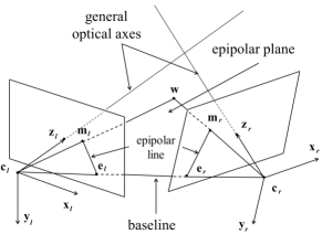
Next, we consider two stereo pinhole cameras as shown in Fig. 2. Let $\mathbf{m_{l}}$ and $\mathbf{m_{r}}$ be point correspondences that are the projections of the same 3D object point $\mathbf{w}$ on images $I_{l}$ and $I_{r}$, respectively. $\mathbf{e_{l}}$ and $\mathbf{e_{r}}$ are called epipoles that are intersection points of the baseline with the left and right image planes. The plane containing the baseline and object point $\mathbf{w}$ is called the epipolar plane, and the intersection lines between the epipolar plane and each of the two image planes are epipolar lines.

The intrinsic projective geometry between the corresponding points in the left and right images can be described by the epipolar constraint as

$$\mathbf{m}_{l}^{T}\mathbf{F}\mathbf{m}_{r}=\mathbf{m}_{r}^{T}\mathbf{F}^{T}\mathbf{m}_{l}=\mathbf{0},$$ (18)

where $\mathbf{F}$ is the fundamental matrix, which is a $3\times 3$ matrix with rank 2, and $\mathbf{0}=\left[0~{}0~{}0\right]^{T}$ is a zero column vector. The epipole, which is the null space of $\mathbf{F}$, satisfies the following condition:

$$\mathbf{F}\mathbf{e}_{l}=\mathbf{F}^{T}\mathbf{e}_{r}=\mathbf{0}.$$ (19)

Fundamental matrix $\mathbf{F}$ maps a point, $\mathbf{m_{l}}$, in one image to the corresponding epipolar line, $\mathbf{Fm_{l}=l_{r}}$, in the other image, upon which the corresponding point $\mathbf{m_{r}}$ should lie. Generally, all epipolar lines are not in parallel with each other and passing through the epipole (namely, $\mathbf{l_{l}^{T}}\mathbf{e}_{l}=\mathbf{l_{r}}^{T}\mathbf{e}_{r}=\mathbf{0}$).

Figure 3: Illustration of image rectification.

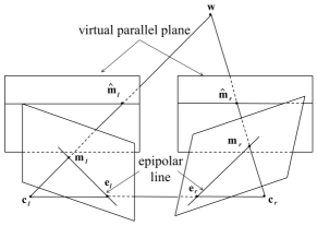
Image rectification as shown in Fig. 3 is the process of converting the epipolar geometry of a given stereo image pair into a canonical form that satisfies two conditions: 1) all epipolar lines are parallel to the baseline, 2) there is no vertical disparity between the corresponding epipolar lines in both images. This can be done by applying homographies to each of image planes or, equivalently, mapping the epipoles to a point at infinity as $\mathbf{e}_{\infty}=[1~{}0~{}0]^{T}$. Especially, the fundamental matrix of a pair of rectified images can be expressed in form of

$$\mathbf{F}_{\infty}=\left[\begin{array}[]{ccc}0&0&0\\ 0&0&-1\\ 0&1&0\end{array}\right].$$ (20)

Let $\mathbf{H_{l}}$ and $\mathbf{H_{r}}$ be two rectifying homographies of the left and right images, respectively, and $(\mathbf{\hat{m}_{l}},\mathbf{\hat{m}_{r}})$ be the corresponding points in the rectified images. Then, we have

$$\mathbf{\hat{m}_{l}}=\mathbf{H}_{l}\mathbf{m}_{l},\phantom{1111}\mathbf{\hat{m}_{r}}=\mathbf{H}_{r}\mathbf{m}_{r}.$$ (21)

According to Eq. (18),

$$\mathbf{\hat{m}_{l}}^{T}\mathbf{F}_{\infty}\mathbf{\hat{m}_{r}}=\mathbf{0}.$$ (22)

By incorporating Eq. (21) in Eq. (22), we obtain

$$\mathbf{m}_{l}^{T}\mathbf{H}_{l}^{T}\mathbf{F}_{\infty}\mathbf{H}_{r}\mathbf{m}_{r}=\mathbf{0}.$$ (23)

As a result, the fundamental matrix of the original stereo image pair can be specified as $\mathbf{F=\mathbf{H}_{l}^{T}\mathbf{F}_{\infty}\mathbf{H}_{r}}$. The fundamental matrix is used to calculate the rectification error in the process of parameter optimization. Thus, the way to parameterize $\mathbf{H_{l}}$ and $\mathbf{H_{r}}$ is critical to the generation of good rectified images.

III Proposed USR-CGD Rectification Algorithm

III-A Generalized Homographies

We begin with a brief review on the parameterization of the homography as proposed by Fusiello et al. [2, 11]. The rectification procedure is a process that defines new virtual cameras $\mathbf{P}_{n_{l}}$ and $\mathbf{P}_{n_{r}}$ given old cameras $\mathbf{P}_{ol}$ and $\mathbf{P}_{or}$. New virtual cameras are obtained by rotating old cameras around their optical centers until two focal planes contain the baseline and become coplanar. The rectifying transformation is used to map the image plane of $\mathbf{P}_{o}$ onto the image plane of $\mathbf{P}_{n}$. Without loss of generality, we use the left camera as the example in the following discussion. The same derivation applies to the right camera as well.

For the left camera, we have

$$\mathbf{H}_{l}=\mathbf{P}_{nl_{1:3}}\mathbf{P}^{-1}_{ol_{1:3}},$$ (24)

where the subscript denotes a range of columns. By Eq. (17), the optical rays of each images can be represented by

$$\mathbf{\hat{w}}_{l} = \mathbf{\hat{c}}_{ol}+\alpha_{ol}\mathbf{R}_{ol}^{-1}\mathbf{K}_{ol}^{-1}\mathbf{m}_{ol},$$ (25)

$$\mathbf{\hat{w}}_{l} = \mathbf{\hat{c}}_{nl}+\alpha_{nl}\mathbf{R}_{nl}^{-1}\mathbf{K}_{nl}^{-1}\mathbf{m}_{nl}.$$ (26)

Since it is assumed that the optical center does not move in old and new camera; namely, $\mathbf{\hat{c}_{ol}=\hat{c}_{nl}}$, in [11], the homography is expressed as

$$\mathbf{H}_{l}=\mathbf{K}_{nl}\mathbf{R}_{l}\mathbf{K}_{ol}^{-1},$$ (27)

where $\mathbf{K}_{ol}$ and $\mathbf{K}_{nl}$ are intrinsic matrices of the old and the new cameras, respectively, and $\mathbf{R}_{l}$ is the rotation matrix that transform the old camera to the new camera for rectification.

(a) Without parameter for y-translation

(b) With parameter for y-translation

Figure 4: The effect of introducing a parameter for the y-translation: the original and rectified stereo pairs are shown in the left and right of subfigures (a) and (b).

The homography model as described above has its limitations since it only allows the rotation around camera’s optical center during the rectification process. However, if there is only vertical disparity between two images, the camera would still be rotated to make focal planes coplanar, which inevitably introduces a warping distortion to the rotated rectified image as shown in Fig. 4(a). Better rectified images can be obtained by allowing an extended set of camera parameters such as the displacement between optical centers and different focal lengths. This is elaborated below.

First, we consider a new homography that includes the translation of the optical center. Based on Eqs. (25) and (26), we get

$$\mathbf{m}_{nl}=\mathbf{K}_{nl}\mathbf{R}_{nl}[\mathbf{c}_{tl}+\mathbf{R}_{ol}^{-1}\mathbf{K}_{ol}^{-1}\mathbf{m}_{ol}],$$ (28)

where $\mathbf{c_{tl}=c_{ol}-c_{nl}}$ denotes the movement between the optical centers of the old and the new cameras. Since the horizontal disparity does not affect the rectification performance, we focus on the case of camera’s vertical translation. The corresponding homography can be derived by simplifying Eq. (28) as

$$\mathbf{H_{l}}=\mathbf{K}_{nl}\mathbf{T_{l}}\mathbf{R_{l}}\mathbf{K}_{ol}^{-1}$$ (29)

where

$$\mathbf{T_{l}}=\left[\begin{array}[]{ccc}1&0&0\\ 0&1&t_{yl}\\ 0&0&1\end{array}\right]$$ (30)

denotes a vertical translation matrix, which compensates the displacement as shown in Fig. 4(b).

Next, we examine another generalization by allowing different focal lengths in two intrinsic matrices. In [11], intrinsic matrices $\mathbf{K}_{ol}$ and $\mathbf{K}_{or}$ are set to be the same, i.e.,

$$\mathbf{K}_{ol}=\mathbf{K}_{or}=\left[\begin{array}[]{ccc}\alpha&0&\frac{w}{2}\\ 0&\alpha&\frac{h}{2}\\ 0&0&1\end{array}\right],$$ (31)

where the same focal length $\alpha$ is adopted. However, if there exists an initial difference in the zoom level between the two cameras, the rectification performance will degrade since two cameras should be rotated on Z-axis to put both image planes to be coplanar as shown in Fig. 5(a), which reults in the up-scaled rectified images in horizontal direction.

(a) Without parameter for z-translation

(b) With parameter for z-translation

Figure 5: The effect of introducing a parameter for different zoom levels: the original and rectified stereo pairs are shown in the left and right of subfigures (a) and (b).

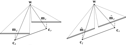
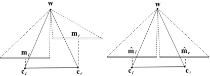
To compensate the initial zoom difference, the left and the right cameras are allowed to have different focal lengths. Thus, we have

$$\mathbf{K}_{ol}=\left[\begin{array}[]{ccc}\alpha_{l}&0&\frac{w}{2}\\ 0&\alpha_{l}&\frac{h}{2}\\ 0&0&1\end{array}\right],\quad\\ \mathbf{K}_{or}=\left[\begin{array}[]{ccc}\alpha_{r}&0&\frac{w}{2}\\ 0&\alpha_{r}&\frac{h}{2}\\ 0&0&1\end{array}\right].$$ (32)

Geometrically, the two image planes are brought to a normalized image plane without loss of perpendicularity with respect to the object point as shown in Fig. 5(b) so that the viewing angle of each camera is not changed.

To summarize, we derive a generalized rectification homograhpy model that consists of nine parameters in this section:

• five rotational parameters: $\theta_{yl}$, $\theta_{zl}$, $\theta_{xr}$, $\theta_{yr}$, and $\theta_{zr}$;

• two y-translational parameters: $t_{yl}$ and $t_{yr}$;

• two focal length parameters: $\alpha_{l}$ and $\alpha_{r}$.

The x-axis rotational parameter ($\theta_{xl}$), which affects the portion of the scene that is projected, is set to zero. Furthermore, since images are projected to the virtual camera plane, we can arbitrarily choose new intrinsic matrices as long as both cameras have the same vertical focal length and the same vertical coordinate of the principal point to meet the epipolar constraint in Eq. (18). Thus, we demand $\mathbf{K}_{nl}$ and $\mathbf{K}_{nr}$ to be the same as the old left one:

$$\mathbf{K}_{nl}=\mathbf{K}_{nr}=\mathbf{K}_{ol}.$$ (33)

III-B Geometric Distortions

The parameters of the rectification homography model are updated through an optimization process to generate a pair of rectified images. There are two measures on the quality of the rectified image: 1) the rectification error and 2) errors of various geometric distortions.

The rectification error is the average vertical disparity in pixels between two corresponding points in the left and right images. It is an objective (or quantitative) measure, and it should be less than 0.5 pixels for a stereo matching algorithm to be performed in the 1-D scanline. In the literature, the Samson error ($E_{s}$) [4, 15] is widely used. It is the approximated projection error defined by

$$E_{s}=\frac{1}{N}\sqrt{\sum_{j=1}^{N}(E_{s})_{j}^{2}},$$ (34)

where $N$ is the number of corresponding pairs and $(E_{s})_{j}$ is the $j$th component of normalized vector $E_{s}$, which is computed via

$$(E_{s})_{j}^{2}=\frac{({m_{r}^{j}}^{T}Fm_{l}^{j})^{2}}{(Fm_{l}^{j})_{1}^{2}+(Fm_{l}^{j})_{2}^{2}+({m_{r}^{j}}^{T}F)_{1}^{2}+({m_{r}^{j}}^{T}F)_{2}^{2}}.$$ (35)

In the image rectification process, we need to define a cost function that takes both the objective quality (as represented by the rectification error $E_{s}$) and the subjective quality (as represented by geometric distortions) into account. The latter is needed since we cannot avoid warping distortions in a perspective transformation. Here, the geometrical distortion is measured by the dissimilarity of a rectified image from its original unrectified one. Several rectification algorithms [5]-[10] have been proposed to control the perspective distortion in rectified images using auxiliary affine transforms (e.g., the Jacobian or SVD of $H$, etc.), yet none of them is clearly superior to others in reaching well-balanced rectification quality.

Mallon and Whelan [8] introduced two geometric measures for performance evaluation: 1) orthogonality and 2) aspect ratio. Let $a=(\frac{w}{2},0,1)^{T}$, $b=(w,\frac{h}{2},1)^{T}$, $c=(\frac{w}{2},h,1)^{T}$ and $d=(0,\frac{h}{2},1)^{T}$ be four mid points of an image before the transform, where $w$ and $h$ are the image width and height. After the transform, the new positions of $a$, $b$, $c$ and $d$ are denoted by $\hat{a}$, $\hat{b}$, $\hat{c}$ and $\hat{d}$, respectively. We examine vectors $\hat{x}=\hat{b}-\hat{d}$ and $\hat{y}=\hat{c}-\hat{a}$. The orthogonality measure is defined as the angle between $\hat{x}$ and $\hat{y}$:

$$E_{O}=\cos^{-1}{\frac{\hat{x}\hat{y}}{\lvert x\lvert\lvert y\rvert}}.$$ (36)

It is desired that the orthogonality measure is as close to $90\degree$ as possible. The aspect ratio is used to measure the ratio of image width to image height before and after the rectification transform. Let $a=(0,0,1)^{T}$, $b=(w,0,1)^{T}$, $c=(w,h,1)^{T}$ and $d=(0,h,1)^{T}$ be the four corner points. Again, we examine vectors $\hat{x}=\hat{b}-\hat{d}$ and $\hat{y}=\hat{c}-\hat{a}$ after the transform. The aspect ratio is defined as

$$E_{A}=(\frac{\hat{x}^{T}\hat{x}}{\hat{y}^{T}\hat{y}})^{1/2}.$$ (37)

The aspect ratio should be as close to unity as possible.

Figure 6: The original and rectified images used to define four new geometric measures.

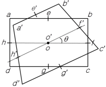
Although $E_{O}$ and $E_{A}$ are useful, they are still not sufficient to characterize all possible geometric distortions in rectified images. For example, $E_{A}$ is sometimes close to the unity in the presence of large skewness. For this reason, we propose four new geometric distortion measures, which includes a modified aspect ratio measure, and use them in the regularization term of the cost function in the optimization process.

We define four corner points ($a$, $b$, $c$ and $d$) and four mid points ($e$, $f$, $g$ and $h$) in the original image as shown in Fig. 6. The points in the rectified image are represented by adding a prime to their symbols. The four new measures are given below.

• Modified aspect ratio (ideally 1):
  

  $$E_{AR}=\frac{1}{2}(\frac{\overline{a^{\prime}o^{\prime}}}{\overline{c^{\prime}o^{\prime}}}+\frac{\overline{b^{\prime}o^{\prime}}}{\overline{d^{\prime}o^{\prime}}}).$$ (38)

  It gives a more accurate measure of the aspect ratio change.

• Skewness (ideally 0°):
  

  $$E_{Sk}=\frac{1}{4}\sum_{i=1}^{4}(\lvert 90\degree-\angle{CA_{i}}\rvert).$$ (39)

  It is used to measure how corner angles (denoted by $\angle CA_{i}$, $i=1,2,3,4$) deviate from 90°after rectification.

• Rotation angle (ideally 0°):
  

  $$E_{R}=\cos^{-1}(\frac{\overline{of}\cdot\overline{o^{\prime}f^{\prime}}}{\lvert\overline{of}\rvert\lvert\overline{o^{\prime}f^{\prime}}\rvert}).$$ (40)

  It is the angle between $\overline{of}$ and $\overline{\tilde{o}\tilde{f}}$, which is used to measure the rotation degree after rectification.

• Size Ratio (ideally 1):
  

  $$E_{SR}=\frac{Area_{rec}}{Area_{orig}}.$$ (41)

  It is used to measure to the size change of the input rectangle after rectification.

The usefulness of the above four geometric distortion measures will be shown in Section V based on extensive experiments.

Generally speaking, the cost function can be written as

$$C(\phi)=E_{s}+\rho_{AR}E_{AR}+\rho_{Sk}E_{Sk}+\rho_{R}E_{R}+\rho_{SR}E_{SR},$$ (42)

where $\phi$ denotes a set of rectification parameters to be selected in the optimization process, $E_{s}$ is the Samson error to characterize the rectification error, and $\rho_{AR}$, $\rho_{Sk}$, $\rho_{R}$ and $\rho_{SR}$ are weights for the modified aspect ratio distortion, the Skewness distortion, the rotation angle distortion and the size ratio distortion, respectively.

III-C Iterative Optimization

To find an optimal solution to Eq. (42) is actually a very challenging task. First, there is a tradeoff between the rectification error and geometric errors. That is, when we attempt to reduce the rectification error by adjusting the parameters of generalized rectification homograhpy $H$, the geometric error tends to increase, and vice versa. As a result, the cost is a non-convex function that has many local minima. Furthermore, the choice of proper weights $\rho_{AR}$, $\rho_{Sk}$, $\rho_{R}$ and $\rho_{SR}$ is an open issue remaining for future research. To proceed, we simply adopt equal weight solution. That is, each weight takes either 0 or 0.25 two values since there is one rectification error term and four geometric error terms in Eq. (42), respectively. For a specific type of geometric distortion, if its error is less than a preset threshold, its weight is set to 0. Otherwise, it is set to 0.25. Mathematically, we have

$$\rho_{X}=\left\{\begin{array}[]{ll}0.25,&\mbox{if }E_{X}\geq T_{X},\\ 0,&\mbox{if }E_{X}<T_{X},\\ \end{array}\right.$$ (43)

where $X$ can be $AR$, $Sk$, $R$ or $SR$ and $T_{X}$ is the corresponding preset threshold.

Figure 7: The block diagram of the proposed iterative optimization procedure.

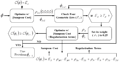
Based on this design, the cost is a dynamically changing function that always contains the rectification error. A geometric distortion term will be included in the cost function (or ”being turned-on”) only when it is larger than a threshold. Otherwise, it is turned off. To solve this problem, we propose an iterative optimization procedure as shown in Fig. 7. It consists of the following steps.

1. We begin with a cost function that contains the Sampson error ($E_{s}$) only. The optimization procedure offers the initial set of rectification parameters, which is denoted by $\phi_{init}$.

2. We update four weight $\rho=(\rho_{AR},\rho_{Sk},\rho_{R},\rho_{SV})$ from $\phi_{init}$, which is initially set to $\rho_{init}=(0,0,0,0)$.

3. Under the current set of rectification parameters, $\phi$, and the current set of weights, $\rho$, we solve the optimization problem with respect to Eq. (42). Then, both rectificatioin parameters and weights are updated accordingly. Step 3 is iterated until the the cost of the current round is greater than or equal to that of the previous round. Mathematically, if $C(\phi_{n})\geq C(\phi_{n-1})$, we choose $\phi_{n-1}$ as the converged rectification parameters.

When we compare the current cost $C(\phi_{n})$ with the cost in the previous round $C(\phi_{n-1})$ in Step 3, the number of geometric terms in Eq. (42) may change. If this occurs, we should compensate it for fair comparison. That is, the cost should be normalized by the sum of weight via $C_{normalized}(\phi_{n})=C(\phi_{n})/(1+\sum_{X}{\rho_{X}})$.

The choice of a proper threshold value for each geometric error is important in reaching balanced performance. In this work, we set threshold values of geometric errors to the following:

$$0.8\leq E_{AR}\leq 1.2, E_{Sk}\leq 5\degree,$$ (44)

$$0.8\leq E_{SV}\leq 1.2, \lvert E_{R}\rvert\leq 30\degree$$ (45)

Furthermore, we normalize four geometric errors by considering their value range. The normalizing factors are:

$$N_{AR}=1.5,\quad N_{Sk}=6.5,\quad N_{R}=18.5,\quad N_{SV}=2.5,$$ (46)

which can be absorbed in their respective weight; i.e. the new weight becomes $\rho_{X}=0.25/N_{X}$ when the term is on. Last, the minimization of the cost function is carried out using the nonlinear least square method, Trust Region [16], starting with all unknown variables set to zero.

Figure 8: The block-diagram of the proposed USR-CGD system.

(a) Interior

(b) Street

(c) Military

(d) Vehicle

Figure 9: The left images of 4 MCL-SS reference image pairs.

(a) Trans. Error on X-axis

(b) Trans. Error on Y-axis

(c) Trans. Error on Z-axis

(d) Compound Error 1

(e) Rot. Error on X-axis

(f) Rot. Error on Y-axis

(g) Rot. Error on Z-axis

(h) Compound Error 2

Figure 10: The 8 test image pairs of “Interior” with different geometric distortions, where left and right images are overlapped for the display purpose.

(a) Doheny

(b) Dog

(c) Dolls

(d) Drawer

(e) Fountain

(f) Keychain

(g) Step

(h) Tommy

Figure 11: The eight selected left images from 20 MCL-RS image pairs.

The block-diagram of the proposed USR-CGD system is shown in Fig. 8. This system is fully automatic since there is no need to estimate the fundamental matrix. To establish the point correspondence between the left and right images, we extract the SIFT feature [17] and find the initial putative matching points. We also apply RANSAC [18] to remove outliers. It is noteworthy that the number of the correspondences strongly affects the rectification performance because the homography is estimated based on their errors, and the optimal number varies with the image resolution. A special case of the USR-CGD algorithm is to turn off all geometric distortion terms, which is called the USR algorithm. We will study the performance of the USR and USR-CGS algorithms in Section V.

IV Databases of Uncalibrated Stereo Images

TABLE I: The databases of uncalibrated stereo images

	MCL databases		Existing databases
Name	MCL-SS	MCL-RS	SYNTIM [19]	VGS [8]
# of Test Images	32	20	8	6
	(8 different geometric distortions per each reference )
Resolution	1920x1080	1920x1080	512x512 or 768x576	640x480
Remark	- CG-images generated from OpenGL programming	- 5 indoor scenes	- 7 indoor scenes	- 2 indoor scenes
		- 15 outdoor scenes	- 1 outdoor scene	- 4 outdoor scenes

The number of publicly available databases of uncalibrated stereo images is small. The SYNTIM database [19] consists of eight stereo images (seven indoor scenes and one outdoor scene) of two resolutions, 512x512 and 768x576. The VSG database [8] consists of six stereo images (two indoor scenes and four outdoor scenes) of resolution 640x480. Although these two databases contain multiple unrectified stereo images taken by different camera poses, it is difficult to analyze the effect of each pose on the quality of rectified images. To allow in-depth analysis, we built two high quality databases of uncalibrated stereo images on our own in this research.

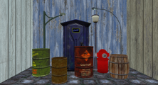
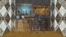
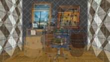
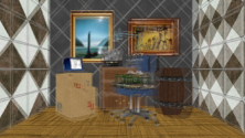
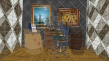
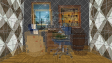
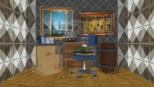
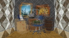
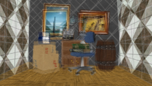
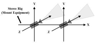
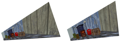
First, we built a synthetic stereo image database consisting of 32 image pairs using the OpenGL programming. The left images of 4 reference stereo pairs are shown in Fig. 9. The advantage of using a synthetic image is that it is easy to generate a specific geometric distortion. Given two cameras whose initial settings are shown in Fig. 12, we can translate or rotate each of cameras along the X-/Y-/Z-axis so as to mimic real world camera configurations such as a converged cameras, a wide baseline, vertical misalignment, and different zoom levels. For each of reference stereo image pairs, we generate 8 test stereo pairs, where 6 of them are obtained by applying a single geometric distortion while 2 are generated by applying all six geometric distortions together. For the latter, we move left and right cameras along the X and Y axes and the range of increased disparity is 0$\sim$185 pixels. The ratio of object’s sizes between left and right images due to cameras’ translation on the Z-axis is about 11.98$\sim$31.24%. Finally, the angle difference due to camera rotation is $10\degree$ on each axis. Eight such image pairs of image “Interior” are given in Fig. 10. More stereo image pairs can be found in  [20].

Figure 12: Camera configuration used to acquire synthetic stereo images.

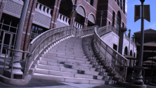
Next, we built a database of unrectified stereo images by capturing various scenes from the real world environment. It consists of 5 indoor scenes and 15 outdoor scenes. The left images of 8 selected scenes are shown in Fig. 11. The scenes were taken with different zoom levels and various poses using two Point Grey Flea3 cameras with an additional zoom lens. To meet the recommendation of the current broadcasting standard, all images were captured in full-HD resolution (1920x1080). For the rest of this paper, we call our synthetic database MCL-SS (synthetic stereo) and the real database MCL-RS (real stereo), where MCL is the acronym of the Media Communication Lab at the University of Southern California. The comparison with existing databases is summarized in Table I. The MCL-SS and MCL-RS databases are accessible to the public [20].

V Performance Evaluation

TABLE II: Performance comparison of six rectification algorithms in terms of the rectification error ($E_{v}$) and orthogonality ($E_{O}$) and Skewness ($E_{Sk}$) geometric distortions, where the best result is shown in bold. For the MCL-SS database, the results of four test sets (Interior, Street, Military, and Vehicle) are averaged.

DATABASE	TEST SET	RECTIFICATION ERROR ($E_{v}$ in pixels)						GEOMETRIC DISTORTIONS (Ideal Value)
								Othogonality (90°)						Skewness (0°˚)
		Hartley	Mallon	Wu	Fusiello	USR	USR-	Hartley	Mallon	Wu	Fusiello	USR	USR-	Hartley	Mallon	Wu	Fusiello	USR	USR-
							CGD						CGD						CGD
MCL-SS	X-translation	0.09	0.13	144.83	0.10	0.09	0.09	91.44	89.96	66.47	90.01	89.95	89.95	1.63	0.36	55.97	0.05	0.34	0.34
	Y-translation	0.09	0.17	1252.36	0.17	0.14	0.69	90.33	45.98	97.39	89.81	90.01	90.19	0.48	44.02	54.23	0.67	0.77	1.69
	Z-translation	0.15	77.26	960.16	0.94	0.24	0.79	100.38	133.94	116.78	92.58	97.74	90.95	27.73	61.14	48.30	5.80	16.56	1.67
	X-rotation	0.09	0.18	246.97	2.13	0.24	0.93	90.40	41.56	132.89	90.22	88.17	89.63	3.75	48.33	48.48	6.85	6.25	3.63
	Y-rotation	0.11	0.20	966.68	0.11	0.08	0.10	91.87	89.17	83.31	90.02	89.97	89.90	4.17	4.14	35.04	3.74	3.75	3.74
	Z-rotation	0.11	0.18	109.49	0.10	0.11	0.09	90.35	92.78	111.08	89.95	90.02	90.10	0.93	3.01	53.95	0.24	0.69	0.70
	compound1	37.52	6443.91	662.73	3.49	0.10	0.55	99.26	110.23	100.38	88.73	97.10	89.98	39.76	31.13	61.06	10.48	18.18	1.45
	compound2	0.10	4.10	101.37	1.32	0.12	0.94	88.36	118.46	95.07	87.47	88.06	89.23	22.32	44.67	52.01	11.97	10.39	2.61
	Mean	4.78	815.76	555.58	1.04	0.25	0.50	92.80	90.26	100.42	89.85	91.39	89.99	12.47	29.60	51.13	4.98	7.11	2.18
MCL-RS	Books	0.68	25.01	129.41	3.47	1.97	1.87	59.91	78.36	43.74	84.95	84.93	91.10	28.47	35.53	43.31	6.38	14.99	4.98
	Dogs	0.21	0.44	2403.43	5.67	0.16	0.17	93.50	93.33	48.66	93.57	89.18	90.21	4.68	5.57	67.57	11.72	2.34	0.99
	Doheny	0.10	0.42	1.75	0.09	0.09	0.08	83.80	80.84	83.45	90.02	88.01	88.96	15.22	11.85	68.85	0.38	4.98	2.56
	Dolls	0.17	1.25	36.09	0.21	0.16	0.20	92.54	100.68	156.50	89.30	93.00	89.69	7.86	10.27	60.14	1.59	8.77	0.92
	Drawer	0.21	0.03	18.50	0.47	0.45	0.20	104.35	134.93	83.80	88.83	92.99	90.04	34.33	43.71	76.14	3.08	27.02	0.14
	Fountain	1.72	36.32	354.99	0.35	0.20	0.91	88.99	87.31	105.04	90.40	90.55	90.32	2.74	2.85	52.19	0.49	1.34	0.86
	Fountain2	0.18	2.66	0.14	2.06	0.20	0.27	94.98	98.58	95.85	82.18	95.36	90.21	10.90	18.48	24.89	15.18	12.31	0.51
	Fountain3	0.27	5.21	169.22	0.14	0.11	0.13	93.45	95.26	133.98	90.16	93.21	90.65	8.32	12.58	53.26	0.32	10.39	1.88
	Fountain4	2.51	9.30	355.94	1.04	1.06	0.45	78.85	50.94	138.19	87.76	81.52	90.21	52.38	43.09	49.54	5.62	21.62	0.75
	Keychain	0.25	1.63	391.80	0.48	0.21	0.42	83.90	87.56	129.47	89.25	84.64	89.45	15.12	12.67	67.26	1.86	2.65	1.65
	Keychain2	0.38	0.57	0.63	12.36	0.23	0.31	88.83	98.50	70.75	77.29	88.90	89.00	2.55	11.76	70.16	13.67	4.17	2.30
	Leavey	0.20	1.37	6.72	0.19	0.11	0.19	90.48	98.29	63.40	89.85	88.37	90.47	2.28	8.40	71.24	0.48	4.55	0.06
	Mudhall	0.15	0.97	0.63	0.12	0.11	0.13	91.40	93.48	116.97	91.42	91.90	89.50	2.04	3.61	23.49	3.36	5.11	1.18
	RTCC	3.27	15.39	0.72	0.27	0.23	0.36	89.62	103.91	103.32	89.31	90.64	89.92	2.76	14.38	58.07	5.75	16.40	1.06
	Salvatory	1.53	7.82	1.30	0.60	0.20	0.56	87.73	87.36	103.62	87.97	85.65	90.47	11.20	9.44	72.15	6.18	5.26	1.11
	Step	1.07	2.98	82.35	0.20	0.78	0.74	94.67	81.95	148.84	96.08	93.40	89.53	9.47	14.84	72.25	9.51	4.46	1.38
	Tommy	0.17	1.41	452.77	0.13	0.11	0.12	89.22	96.86	90.07	89.92	88.03	90.06	1.97	8.66	0.00	0.28	7.65	1.07
	Tommy2	0.14	5.39	346.31	0.13	0.10	0.11	91.39	93.90	31.32	90.34	90.94	90.15	5.07	6.54	51.28	3.22	9.17	0.20
	Viterbi	0.12	0.33	0.59	0.12	0.37	0.11	93.23	86.30	64.80	89.98	86.17	90.15	17.93	27.96	40.49	0.39	0.56	1.64
	VKC	0.20	0.62	2527.03	0.17	0.17	0.15	84.99	81.27	37.77	90.00	89.73	89.31	9.27	9.97	49.77	0.16	4.19	1.58
	Mean	0.67	5.96	364.02	1.41	0.31	0.38	88.84	91.48	92.15	88.92	89.28	89.96	12.23	15.61	55.21	4.48	8.98	1.34
SYNTIM	Aout	0.33	2.67	11.43	4.32	0.53	1.44	99.68	110.98	88.99	86.70	92.94	91.09	21.47	26.12	65.47	14.92	11.49	7.41
	BalMire	0.46	3.21	256.49	0.45	0.22	0.34	90.77	96.39	133.71	91.20	91.24	89.66	11.10	14.24	52.66	3.87	11.17	2.95
	BalMouss	0.19	0.33	0.19	0.21	0.18	0.26	91.64	84.67	88.53	88.68	88.56	89.46	6.76	5.29	6.03	4.89	5.39	2.42
	BatInria	0.15	0.47	0.15	0.14	0.13	0.13	90.69	87.31	89.99	90.00	89.93	89.98	3.47	3.35	6.18	1.26	4.09	2.35
	Color	0.20	0.32	0.21	0.42	0.19	0.43	95.56	85.71	89.99	88.76	89.95	90.14	7.91	5.74	6.29	7.31	5.06	2.69
	Rubik	0.14	1.24	1.42	0.41	0.13	0.38	87.26	108.58	58.40	89.84	93.97	91.17	14.24	17.51	56.94	0.43	11.74	0.42
	Sport	0.13	0.94	0.56	0.06	0.07	0.08	73.58	79.25	135.17	90.84	87.50	90.00	49.88	27.26	64.71	3.18	9.56	0.10
	Tot	0.14	0.80	0.61	0.24	0.15	0.73	83.87	74.82	63.86	86.20	86.47	88.06	16.52	14.99	54.44	15.10	13.81	10.78
	Mean	0.22	1.25	33.88	0.78	0.20	0.47	89.06	90.96	93.58	89.03	90.07	89.82	16.42	14.31	39.09	6.37	9.04	3.64
VSG	Arch	0.18	0.55	67.15	0.17	0.15	0.17	88.63	85.59	76.44	90.63	87.94	90.42	20.28	13.77	28.67	2.08	6.88	1.01
	Drive	28.16	0.56	44.87	0.17	0.17	0.16	97.08	99.16	130.15	89.22	87.47	89.98	26.40	19.95	51.11	4.29	9.94	0.18
	Lab	0.11	0.27	1.22	0.09	0.08	0.10	86.19	101.45	86.21	91.34	91.39	91.14	6.81	11.38	78.11	4.84	4.84	4.15
	Roof	0.14	0.14	86.01	0.62	0.11	0.32	111.39	93.25	91.45	91.64	90.02	90.71	23.81	7.57	5.93	3.71	6.24	3.83
	Slate	0.20	0.15	2.21	0.11	0.11	0.18	88.76	83.66	88.43	88.92	88.28	89.98	7.01	6.30	76.09	4.33	6.89	0.42
	Yard	0.20	0.38	0.14	0.11	0.10	0.13	94.60	84.42	87.03	89.28	88.43	89.73	10.24	7.81	14.11	5.02	7.30	1.52
	Mean	5.12	0.34	33.60	0.21	0.12	0.18	94.44	91.26	93.28	90.17	88.92	90.33	15.76	11.13	42.34	4.04	7.01	1.85

TABLE III: Performance comparison of six rectification algorithms in terms of aspect-ratio ($E_{AR}$). rotation ($E_{R}$) and scale-variance ($E_{SR}$) geometic distortions, where the best result is shown in bold. For the MCL-SS database, the results of four test sets (Interior, Street, Military, and Vehicle) are averaged.

DATABASE	TEST SET	GEOMETRIC DISTORTIONs (Ideal Value)
		Aspect-Ratio (1)						Rotation (0°)						Scale-Variance (1)
		Hartley	Mallon	Wu	Fusiello	USR	USR-	Hartley	Mallon	Wu	Fusiello	USR	USR-	Hartley	Mallon	Wu	Fusiello	USR	USR-
							CGD						CGD						CGD
MCL-SS	X-translation	1.01	1.01	95.57	1.00	1.00	1.00	0.17	45.13	50.93	0.02	0.17	0.17	1.00	1.00	8.43	1.00	1.00	1.00
	Y-translation	1.01	1.01	248.66	1.01	1.02	1.03	54.17	93.47	87.24	53.13	56.87	42.76	1.01	1.25	288.82	1.02	1.03	1.02
	Z-translation	3.11	2.86	28.94	2.20	2.82	1.03	37.37	73.18	90.10	2.43	17.58	2.39	4.55	0.21	27.68	31.65	12.04	1.12
	X-rotation	1.16	1.21	1231.26	1.23	2.82	1.15	56.35	79.69	71.88	54.72	60.26	51.57	1.03	1.46	2.17	1.21	1.01	1.05
	Y-rotation	1.08	1.08	129.90	1.08	1.08	1.07	1.68	16.31	33.63	1.65	1.64	1.63	1.00	1.07	78.58	1.04	1.08	1.07
	Z-rotation	1.01	1.01	417.89	1.00	1.00	1.01	5.19	5.22	100.49	5.18	5.19	5.17	1.01	0.99	0.40	1.00	1.00	1.00
	compound1	5.12	2.63	400.24	1.38	1.58	1.03	64.19	57.39	87.66	16.91	23.01	15.87	1.36	5.98	219.74	1.28	2.47	1.06
	compound2	3.43	2.57	426.15	1.34	1.32	1.08	48.80	65.84	67.65	39.71	50.57	46.19	4.60	1.20	18.05	1.09	1.44	0.98
	Mean	2.11	1.67	372.33	1.28	1.38	1.05	33.49	54.53	73.70	22.47	26.91	21.12	1.94	1.65	80.48	4.91	2.01	1.03
MCL-RS	Books	6.21	10.51	20.05	1.11	2.94	1.08	81.76	89.62	70.90	14.34	86.06	38.32	0.92	80.26	7.06	1.26	10.41	1.14
	Dogs	1.05	1.05	3.32	2.14	1.04	1.02	8.99	7.51	90.79	4.72	8.89	8.88	1.19	0.97	0.93	2.13	0.83	0.84
	Doheny	1.31	1.31	56.69	1.01	1.10	1.05	7.25	86.51	16.47	7.36	6.69	7.16	0.66	1.52	0.67	1.00	1.00	0.98
	Dolls	1.19	1.19	4.40	1.03	1.24	1.03	8.32	9.43	148.80	7.22	8.21	3.26	1.34	0.75	0.43	1.01	1.57	0.95
	Drawer	15.93	7.48	29.39	1.13	11.79	1.00	22.66	67.89	82.86	0.80	64.30	0.05	81.95	0.16	1.68	2.99	12.54	0.85
	Fountain	1.05	1.06	63.33	1.04	1.03	1.03	4.83	34.04	73.16	61.09	99.08	20.80	0.94	1.09	4.24	1.03	1.04	1.02
	Fountain2	1.34	1.34	1.85	1.75	1.75	1.02	7.26	87.23	13.88	7.53	6.95	2.35	1.30	0.81	1.75	4.11	7.57	1.12
	Fountain3	1.30	1.29	896.51	1.01	2.26	1.04	5.44	60.61	46.86	6.32	8.73	5.66	1.44	0.80	3.93	1.00	11.96	1.07
	Fountain4	20.33	3.62	18.19	1.21	2.78	1.01	43.01	163.92	104.06	4.39	33.87	4.24	8.14	4.46	9.01	2.88	9.34	0.80
	Keychain	1.35	1.34	2589.48	1.04	1.33	1.09	4.78	4.34	115.30	7.53	4.52	7.42	0.81	1.63	101.40	0.99	1.32	0.98
	Keychain2	1.05	1.05	138.23	1.17	1.05	1.04	9.68	36.37	81.10	2.13	9.68	9.62	0.77	1.24	0.84	4.30	1.41	1.41
	Leavey	1.05	1.06	35.07	1.01	1.10	1.00	13.26	45.83	57.89	18.73	26.34	5.70	1.04	0.96	1.91	1.00	1.03	1.00
	Mudhall	1.04	1.04	141.11	1.08	1.10	1.06	4.76	4.98	10.76	4.02	5.43	3.91	1.02	0.96	0.66	1.13	1.27	1.04
	RTCC	1.05	1.06	352.77	1.13	1.13	1.07	16.40	38.97	87.48	27.42	29.73	25.09	1.02	0.96	0.00	1.09	1.24	0.98
	Salvatory	1.27	1.27	135.96	1.20	1.60	1.05	6.98	35.86	97.01	11.34	8.60	13.00	0.85	1.41	5.03	1.19	1.56	1.00
	Step	1.24	1.24	1311.56	1.31	1.12	1.03	12.60	84.80	133.00	37.01	38.13	11.94	1.36	0.75	419.14	1.43	1.33	1.01
	Tommy	1.04	1.04	1.00	1.01	1.09	1.04	13.87	39.54	0.00	15.59	13.63	15.06	1.01	1.07	1.00	1.00	0.96	0.98
	Tommy2	1.11	1.11	700.69	1.09	1.18	1.02	6.52	7.03	5.39	7.17	7.70	6.52	1.07	0.95	2.77	1.22	1.38	1.00
	Viterbi	30.28	28.85	2.06	1.03	31.69	1.03	14.20	80.41	42.90	56.21	0.22	1.96	32.15	0.85	1.76	1.00	19.25	1.02
	VKC	1.20	1.20	124.81	1.02	1.08	1.04	9.87	35.51	70.13	8.56	8.04	8.39	0.86	1.28	0.19	1.00	0.98	0.98
	Mean	4.57	3.46	348.02	1.17	3.47	1.04	15.00	51.02	69.14	12.77	26.53	9.97	6.99	5.14	29.28	1.64	12.03	1.01
SYNTIM	Aout	5.32	2.31	1114.30	3.64	2.19	1.65	27.80	86.77	125.85	22.89	33.56	25.99	2.54	1.20	0.02	1.25	2.01	1.08
	BalMire	1.40	1.40	3.59	1.12	1.77	1.08	6.93	53.02	63.67	2.83	8.02	3.24	1.12	0.99	1.50	1.37	4.97	1.08
	BalMouss	1.16	1.16	1.17	1.15	1.16	1.06	5.67	48.26	4.88	4.16	4.40	3.03	0.95	1.23	1.09	1.12	1.07	0.93
	BatInria	1.14	1.14	1.25	1.05	1.16	1.09	0.95	45.93	1.31	1.70	1.38	1.26	1.06	1.22	1.28	1.01	1.18	1.07
	Color	1.24	1.24	1.26	1.42	1.24	1.10	5.15	47.16	5.05	3.84	4.75	4.85	1.09	1.37	1.23	1.57	1.31	1.01
	Rubik	1.47	1.51	14.07	1.01	1.51	1.01	17.53	89.82	87.59	7.70	13.73	8.07	1.25	0.55	2.48	1.01	2.16	1.00
	Sport	5.86	4.42	21.63	1.09	1.34	1.00	13.84	47.74	120.32	1.52	6.21	0.03	1.67	13.77	7.16	1.03	1.70	1.00
	Tot	1.66	1.77	22.56	1.65	1.67	1.45	21.75	91.28	67.78	19.37	17.26	16.99	0.79	2.71	46.42	1.04	1.47	1.32
	Mean	2.41	1.87	147.48	1.52	1.50	1.18	12.45	63.75	59.55	8.00	11.16	7.93	1.31	2.88	7.65	1.18	1.98	1.06
VSG	Arch	10.88	3.70	1.52	1.06	1.24	1.03	6.62	32.15	57.21	3.52	2.87	3.46	3.08	13.50	1.07	1.02	1.30	1.02
	Drive	11.66	1.60	34.84	1.16	1.45	1.00	32.70	46.59	93.17	3.86	5.85	1.62	3.01	1.53	7.18	1.42	2.72	1.00
	Lab	1.13	1.14	134.37	1.14	1.14	1.11	16.57	19.62	86.08	16.86	16.71	16.44	1.11	0.86	26.94	1.06	1.16	1.14
	Roof	1.20	1.20	1.18	1.12	1.19	1.15	1.27	89.40	1.01	1.09	1.16	1.38	1.15	0.75	0.85	1.60	1.31	1.14
	Slate	1.20	1.20	25.26	1.12	1.21	1.01	10.86	36.13	89.51	10.12	6.12	5.69	0.89	1.32	2.28	0.99	1.16	0.98
	Yard	1.27	1.27	1.42	1.26	1.03	1.04	2.72	30.94	3.28	2.30	2.42	2.49	0.92	1.46	1.46	1.09	1.40	1.01
	Mean	4.56	1.68	33.10	1.25	1.06	1.05	11.76	42.47	55.04	6.29	6.51	5.18	1.69	3.24	6.64	1.20	1.51	1.05

To evaluate the performance of the proposed USR and USR-CGD algorithms, we compare them with four rectification algorithms over the four databases described in Section IV. The four benchmark algorithms are Hartley [4], Mallon and Whelan [8], Wu and Yu [10] and Fusiello and Luca [11]. We adopt the following vertical disparity error

$$E_{v}=\frac{1}{N}\sum_{j=1}^{N}(E_{v})_{j},$$ (47)

where

$$(E_{v})_{j}=|(H_{l}m_{l}^{j})_{2}-(H_{r}m_{r}^{j})_{2}|,$$ (48)

as the objective error measure while orthogonality ($E_{O}$), aspect-ratio ($E_{AR}$), skewness ($E_{Sk}$), rotation ($E_{R}$), and scale-variance ($E_{SV}$) are used as subjective error measures. For the number of correspondences, different numbers of matching points are adopted for different image resolutions; namely, 300 for the MCL-SS and the MCL-RS databases (1920x1080), 80 for the SYNTIM database (512x512 or 768x576), and 50 for the VSG database (640x480), respectively. Note that the number of correspondences may decrease after outlier removal.

To obtain more reliable results, we conduct experiments on each test set with three random seeds for RANSAC, which results in different distributions of correspondences. Then, these results are averaged for the final performance measure. Each geometric error is the averaged value of left and right rectified images. Extensive experimental results are shown in Tables II and III, where the best algorithm is marked in bold. Note that these two tables contain the same horizontal entries but different vertical entries. The rectification error, the orthogonality and skewness distortions are shown in Table II while the aspect ration, rotation and scale variance distortions are shown in Table III.

We first examine the advantages of the generalized homography model without considering the geometric distortion constraints (namely, the USR algorithm). At the bottom of each test set in Table  II, we show the mean performance for that particular set. As far as the rectificatoin error is concerned, we see that the USR algorithm provides the smallest error for all four databases.

The results of the MCL-SS database allow us to analyze the performance improvement. To give an example, the vertical disparity is often caused by translational distortion in the Y-axis, rotational distortion in the X-axis and different zoom levels in the Z-axis (emulated by translational distortion). By comparing our generalized homography model with that of Fuesillo and Luca [11], our model provides smaller errors in all three cases since it includes additional degrees of freedom to compensate geometric errors. Furthermore, two stereo paris with compound distortions are challenging to existing algorithms while the USR algorithm offers a stable and robust performance across all test pairs since the generalized homography model is able to cope with combined geometric distortions.

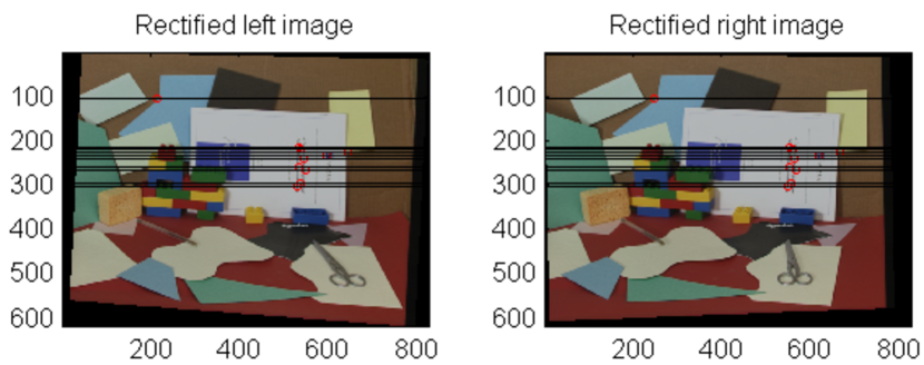
On the other hand, the USR algorithm does not offer the best performance in geometric distortions since it does not take them into consideration. As shown in Tables II and III, the USR-CGD algorithm has the lowest geometric distortions in most cases. For subjective quality comparison, we show a rectified image pair using the USR and USR-CGD algorithms in Fig. 13. Although the rectification error ($E_{v}$) of the USR-CGD algorithm increases slightly (from 0.12 to 0.34 pixel), its resulting image pair look much more natural since all geometric errors are reduced significantly.

Generally speaking, the rectification error of the USR-CGD algorithm is comparable with that of the USR algorithm, and the increase of $E_{v}$ in the USR-CGD algorithm is around $0.06\sim 0.27$ pixels. Among the six benchmarking algorithms, only USR and USR-CGD achieve a mean rectification error ($E_{v}$) less than 0.5 pixel, which is the minimum requirement for stereo matching to be performed along the 1D scanline.

(a) The rectified image pair using the USR algorithm ($E_{v}$=0.12)

(b) The rectified image pair using the USR-CGD algorithm ($E_{v}$=0.34)

Figure 13: Subjective quality comparison of rectified image pair using (a) the USR algorithm and (b) the USR-CGD algorithm.

TABLE IV: Performance comparison based on 100 and 300 correspondences as the input.

Database		MCL-SS						MCL-RS
Algorithm	# of	$E_{v}$	Geometric Errors					$E_{v}$	Geometric Errors
	Correspondences		$E_{O}$	$E_{Sk}$	$E_{AR}$	$E_{R}$	$E_{SR}$		$E_{O}$	$E_{Sk}$	$E_{AR}$	$E_{R}$	$E_{SR}$
Hartley	300	4.78	92.80	12.47	2.11	33.49	1.94	0.67	88.84	12.23	4.57	15.00	6.99
	100	2202.55	93.12	15.24	8.90	38.42	18.59	110.13	86.55	16.75	3.07	24.96	3.24
Mallon	300	815.76	90.26	29.60	1.67	54.53	1.65	5.96	91.48	15.61	3.46	51.02	5.14
	100	13266.94	87.72	31.39	2.30	59.87	1.94	19.72	88.98	19.97	2.27	51.77	2.23
Wu	300	555.58	100.42	51.13	372.33	73.70	80.48	364.02	92.15	55.21	348.02	69.14	29.28
	100	1039.03	94.99	48.54	1070.51	82.34	9.47	1231.28	83.41	60.53	400.13	74.88	150.88
Fusiello	300	1.04	89.85	4.98	1.28	21.47	4.91	1.41	88.92	4.48	1.17	12.77	1.64
	100	119.49	89.19	5.72	1.40	20.38	5.56	1.13	89.17	3.34	1.11	13.60	1.56
USR-CGD	300	0.50	89.99	2.18	1.05	24.12	1.03	0.38	89.96	1.34	1.04	9.97	1.01
	100	0.52	90.01	2.88	1.01	23.28	1.04	0.26	90.00	1.36	1.04	10.17	1.03

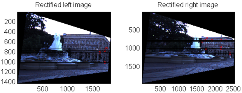
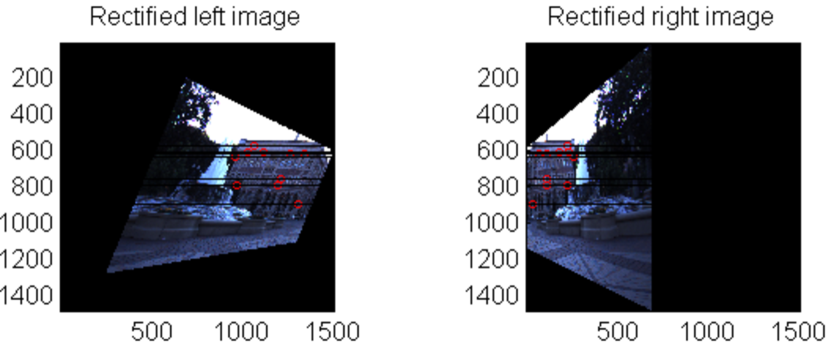
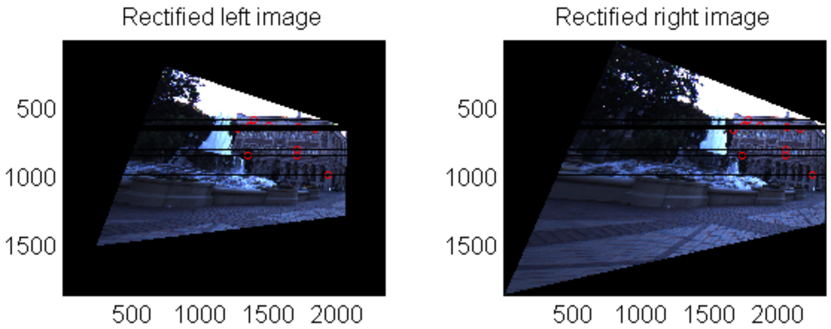
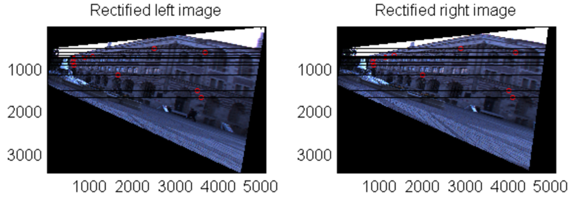
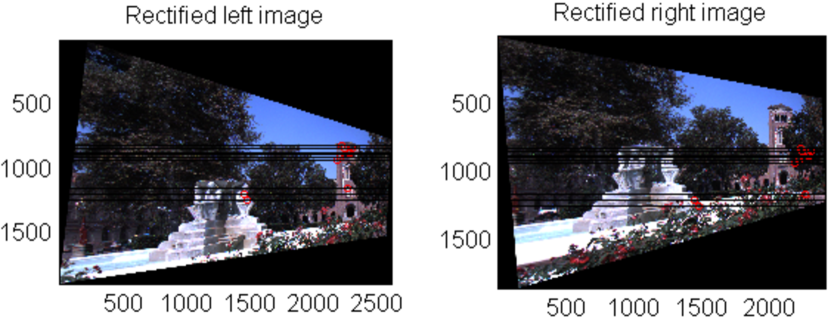
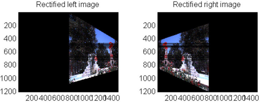
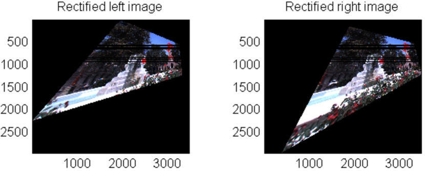
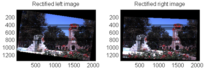
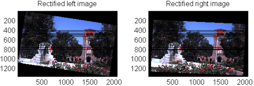
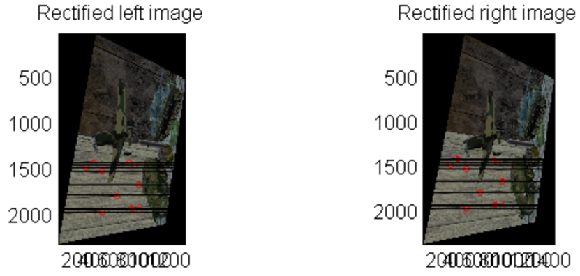
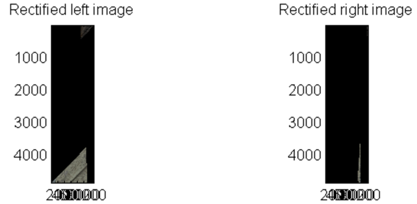
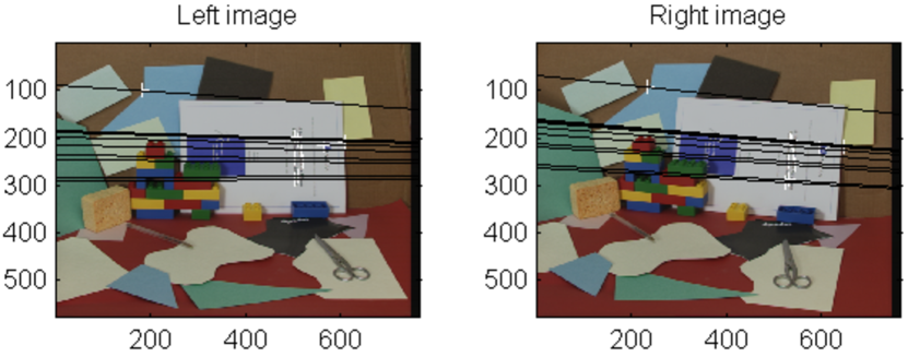
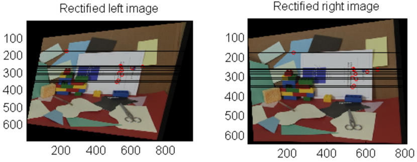
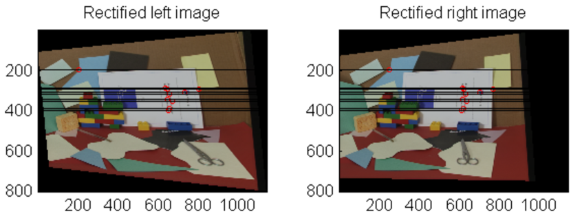
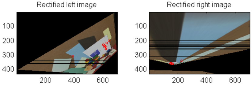
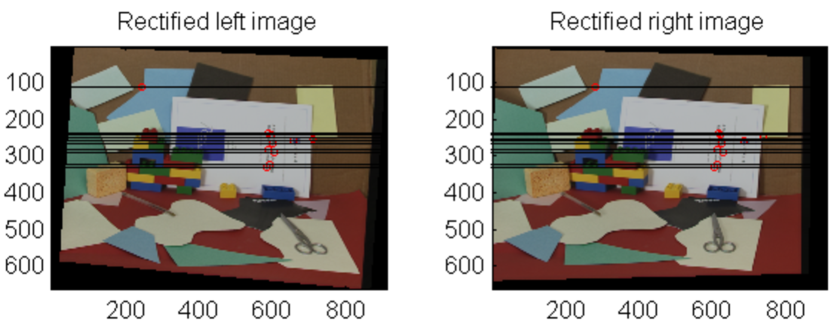
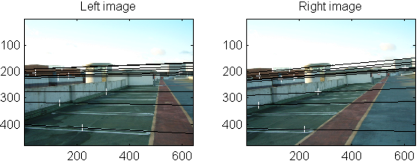
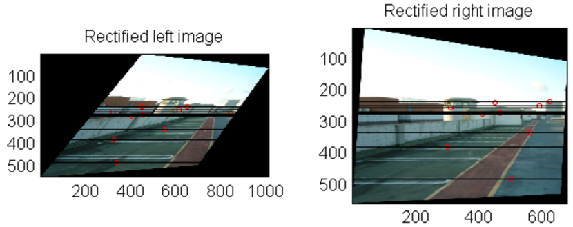
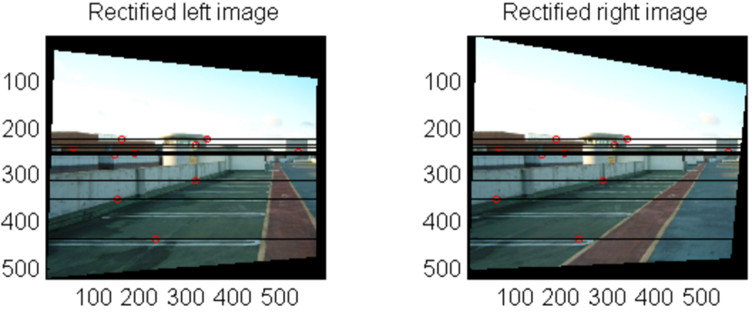
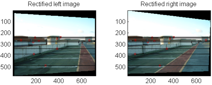
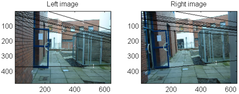
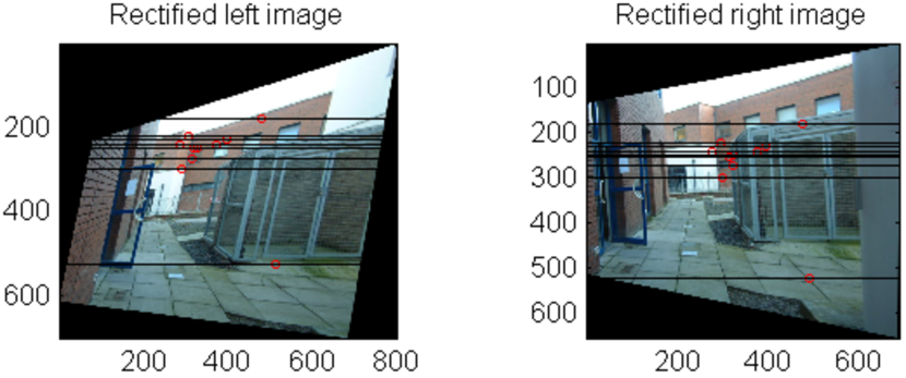
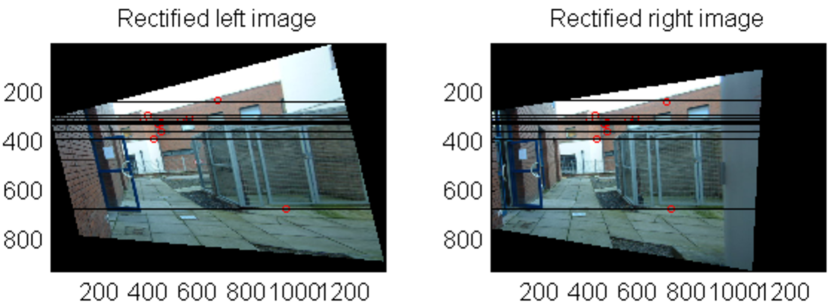
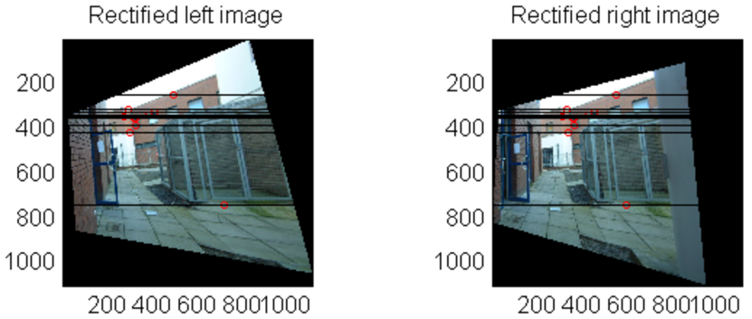
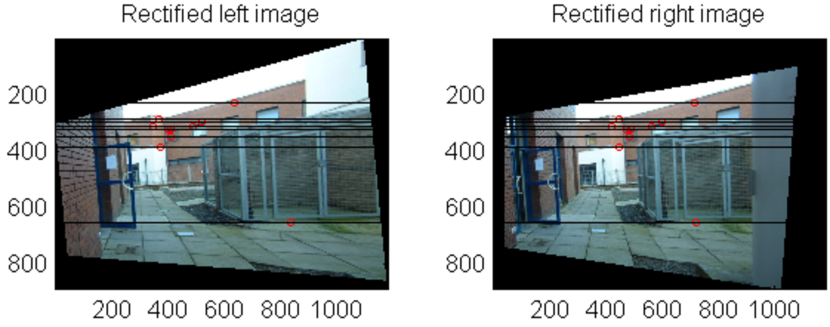
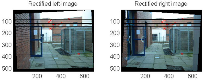
For the subjective quality evaluation of rectified stereo image pairs of the proposed USR-CGD algorithm and four benchmarking algorithms, we select six representative images pairs and show their rectified results in Figs. 14$\sim$19. The vertical disparity error $E_{v}$ is also listed for each subfigure. For the purpose of displaying $E_{v}$, we choose ten sample matching points, which are evenly distributed along the vertical direction and draw corresponding epipolar lines. It is apparent that the proposed USR-CGD algorithm have the best visual quality with minimal warping distortion at the cost of slightly higher rectification errors in some cases.

There is another advantage of the USR-CGD algorithm. That is, it is able to provide robust performance when the number of correspondences is smaller. To demonstrate this, we conduct the same test with 100 correspondences for the MCL-SS and MCL-RS databases. The performance comparison of using 300 and 100 correspondences is shown in Table IV. The rectification errors of all four benchmarking algorithms increase a lot since their reliability in point matching is more sensitive to the number of correspondences. In contrast, the USR-CGD algorithm still maintains the rectification error at a similar level. This is because that the USR-CGD algorithm can adaptively optimize the homographies to meet pre-set conditions. A similar behavior is also observed in the degree of geometric distortions.

Based on the above discussion, we conclude that the USR-CGD algorithm achieves the best overall performance in finding a proper balance between the rectification error and geometric distortions since it includes all of them in its objective function for optimization.

(a) Original unrectified image pair

(b) Hartley ($E_{v}$=0.146)

(c) Mallon ($E_{v}$=1.504)

(d) Wu ($E_{v}$=0.193)

(e) Fuesillo ($E_{v}$=2.109)

(f) USR-CGD ($E_{v}$=0.199)

Figure 14: Comparison of subjective quality and rectification errors for Fountain2 in the MCL-RS database.

(a) Original unrectified image pair

(b) Hartley ($E_{v}$=0.214)

(c) Mallon ($E_{v}$=5.484)

(d) Wu ($E_{v}$=4.520)

(e) Fuesillo ($E_{v}$=0.120)

(f) USR-CGD ($E_{v}$=0.101)

Figure 15: Comparison of subjective quality and rectification errors for for Fountain3 in the MCL-RS database.

(a) Original unrectified image pair

(b) Hartley ($E_{v}$=0.061)

(c) Mallon ($E_{v}$=625.942)

(d) Wu ($E_{v}$=99.432)

(e) Fuesillo ($E_{v}$=0.133)

(f) USR-CGD ($E_{v}$=0.127)

Figure 16: Comparison of subjective quality and rectification errors for Military in the MCL-SS database.

(a) Original unrectified image pair

(b) Hartley ($E_{v}$=0.141)

(c) Mallon ($E_{v}$=0.796)

(d) Wu ($E_{v}$=0.607)

(e) Fuesillo ($E_{v}$=0.240)

(f) USR-CGD ($E_{v}$=0.308)

Figure 17: Comparison of subjective quality and rectification errors for Tot in the SYNTIM database.

(a) Original unrectified image pair

(b) Hartley ($E_{v}$=0.108)

(c) Mallon ($E_{v}$=0.127)

(d) Wu ($E_{v}$=0.091)

(e) Fuesillo ($E_{v}$=1.068)

(f) USR-CGD ($E_{v}$=0.282)

Figure 18: Comparison of subjective quality and rectification errors for Root in the VSG database.

(a) Original unrectified image pair

(b) Hartley ($E_{v}$=0.098)

(c) Mallon ($E_{v}$=0.385)

(d) Wu ($E_{v}$=0.125)

(e) Fuesillo ($E_{v}$=0.128)

(f) USR-CGD ($E_{v}$=0.119)

Figure 19: Comparison of subjective quality and rectification errors for Yard of in the VSG database.

VI Conclusion and Future Work

A new rectification algorithm, called USR-CGD, was proposed for uncalibrated stereo images in this work. It adopts a generalized homography model to reduce the rectification error and incorporates several practical geometric distortions in the cost function as regularization terms, which prevent severe perspective distortions in rectified images. It was shown by experimental results that the proposed USR-CGD algorithm outperforms existing algorithms in both objective and subjective quality measures. In the future, we would like to study the stereo matching problem for depth estimation based on the current work on uncalibrated stero image rectification.

VII Acknowledgements

This work was funded by SAIT (Samsung Advanced Institute of Technology) and supported in part by the University of Southern California Center for High-Performance Computing and Communications. The use of Matlab functions by Dr. A. Fusiello, SYNTIM (INRIA, Rocquencourt) images (http://www-rocq.inria.fr/$\sim$tarel/syntim/paires.html) and VSG (Vision Systems Group, Dublin CityUniversity) images (http://www.vsg.dcu.ie/code.html) is gratefully appreciated.

References

- [1] N. Ayache, and L. Francis, “Trinocular stereo vision for robotics.” in IEEE Transactions on Pattern Analysis and Machine Intelligence, vol. 13, no. 1, pp 73-85, 1991.
- [2] A. Fusiello, T. Emanuele, and V. Alessandro, “A compact algorithm for rectification of stereo pairs.” in Machine Vision and Applications, vol.12, no. 1, pp. 16-22, 2000.
- [3] R. Hartley, “Theory and practice of projective rectification.” in Internat. J. Comput. Vision, vol. 35, no. 2, pp. 115-127, 1999.
- [4] R. Hartley, and Z. Andrew, “Multiple view geometry in computer vision.” in Cambridge university press, 2003.
- [5] C. Loop, and Z. Zhang, “Computing rectifying homographies for stereo vision.” in Proceedings of the IEEE Conference on Computer Vision and Pattern Recognition, vol. 1, pp. 125–131, Jun, 1999.
- [6] M. Pollefeys, K. Reinhard, and G. Luc, “A simple and efficient rectification method for general motion.” in Proceedings of the IEEE Conference on Computer Vision and Pattern Recognition, Vol. 1. pp. 496-501, 1999.
- [7] J. Gluckman, and S. Nayar. “Rectifying transformations that minimize resampling effects” in Proceedings of the IEEE Conference on Computer Vision and Pattern Recognition, vol. 1, pp. 111–117, Dec, 2001.
- [8] J. Mallon, and P. Whelan, “Projective rectification from the fundamental matrix.” in Image and Vision Computing, vol. 23, no.7, pp. 643-650, 2005. (VSG images can be downloadable at: http://www.vsg.dcu.ie/code.html)
- [9] F. Isgrò, and T. Emanuele, “On robust rectification for uncalibrated images.” in IEEE International Conference on Image Analysis and Processing, pp. 297-302, 1999.
- [10] H. Wu, and Y. Yu. “Projective rectification with reduced geometric distortion for stereo vision and stereoscopic video.”, in Journal of Intelligent and Robotic Systems, vol. 42, no. 1, pp. 71-94, 2005.
- [11] A. Fusiello, and I. Luca, “Quasi-Euclidean epipolar rectification of uncalibrated images.” in Machine Vision and Applications, vol. 22, no. 4, pp. 663-670, 2011.
- [12] F. Zilly, M. Müller, P. Eisert, and P. Kauff, “Joint estimation of epipolar geometry and rectification parameters using point correspondences for stereoscopic TV sequences.” in Proceedings of 3DPVT, Paris, France, 2010.
- [13] M. Georgiev, G. Atanas, and H. Miska, “A fast and accurate re-calibration technique for misaligned stereo cameras.” in IEEE International conference on Image Processing, pp. 24-28, 2013.
- [14] O. Faugeras, “Three-dimensional computer vision: a geometric viewpoint”, MIT press, Cambrigde, MA, 1993.
- [15] Q. Luong, and D. Olivier, “The fundamental matrix: Theory, algorithms, and stability analysis.” in International Journal of Computer Vision Vol. 17, No. 1, pp. 43-75, 1996.
- [16] Y. Yuan, “A review of trust region algorithms for optimization.” in ICIAM, Vol. 99, 2000.
- [17] G. Lowe, “Distinctive image features from scale-invariant keypoints.” in International journal of computer vision. Vol. 60, no. 2, pp. 91-110, 2004.
- [18] M. Fischler, and R. Bolles, “Random sample consensus: a paradigm for model fitting with applications to image analysis and automated cartography.” in Communications of the ACM, Vol. 24, no. 6, pp. 381-395, 1881.
- [19] SYNTIM images can be downloadable at: “http://perso.lcpc.fr/tarel.jean-philippe/syntim/paires.html”
- [20] MCL-SS & MCL-RS databases can be downloadable at : http://mcl.usc.edu/mcl-ss-database/ and http://mcl.usc.edu/mcl-rs-database/