Generalized ridge estimator and model selection criterion in multivariate linear regression

Yuichi Mori111Department of Mathematical and Computing Sciences Graduate School of Information Science and Engineering Tokyo Institute of Technology, Taiji Suzukiβˆ—222PRESTO,JST
Abstract

We propose new model selection criteria based on generalized ridge estimators dominating the maximum likelihood estimator under the squared risk and the Kullback-Leibler risk in multivariate linear regression. Our model selection criteria have the following favorite properties: consistency, unbiasedness, uniformly minimum variance. Consistency is proven under an asymptotic structure pnβ†’c→𝑝𝑛𝑐\frac{p}{n}\to c where n𝑛n is the sample size and p𝑝p is the parameter dimension of the response variables. In particular, our proposed class of estimators dominates the maximum likelihood estimator under the squared risk even when the model does not include the true model. Experimental results show that the risks of our model selection criteria are smaller than the ones based on the maximum likelihood estimator and that our proposed criteria specify the true model under some conditions.

1 Introduction

Model selection criteria such as AIC (Akaike, (1971)) and Cp (Mallows, (1973)) have been used in various applications and their theoretical properties have been extensively studied. We consider a model selection problem in a multivariate linear regression based on a kind of generalized ridge estimators. The multivariate linear regression considered in this paper has p𝑝p response variables on a subset of kπ‘˜k explanatory variables, and the response is contaminated by a multivariate normal noise. This model, in which the response is multivariate, is thus an extension of multiple linear regression, where the response is univariate. Applications of multivariate linear regression include genetic data analysis, (e.g., Gharagheizi, (2008)) and multiple brain scans (e.g., Basser and Pierpaoli, (1998)). Multivariate linear regression is written as

YβˆΌπ’©nΓ—p​(A​B,Ξ£βŠ—In),similar-toπ‘Œsubscript𝒩𝑛𝑝𝐴𝐡tensor-productΞ£subscriptI𝑛\displaystyle Y\sim{\cal N}_{n\times p}(AB,\Sigma\otimes\mathrm{I}_{n}),

where Yπ‘ŒY is an nΓ—p𝑛𝑝n\times p observation matrix of p𝑝p response variables, A𝐴A is an nΓ—kπ‘›π‘˜n\times k observation matrix of kπ‘˜k explanatory variables, B𝐡B is a kΓ—pπ‘˜π‘k\times p unknown matrix of regression coefficients, ΣΣ\Sigma is a pΓ—p𝑝𝑝p\times p unknown covariance matrix, kπ‘˜k is a nonstochastic number, and n𝑛n is the sample size. We assume that, for all nβ‰₯kπ‘›π‘˜n\geq k, nβˆ’pβˆ’kβˆ’1>0π‘›π‘π‘˜10n-p-k-1>0 and that rank​(A)=krankπ΄π‘˜\mathrm{rank}(A)=k.

The purpose of the model selection problem is to select an appropriate subset of regression coefficients. Suppose that J𝐽J denotes a subset of the index set of coefficients F={1,…,k}𝐹1β€¦π‘˜F=\{1,...,k\}. π’₯π’₯{\cal J} denotes the power set of F𝐹F, and kJsubscriptπ‘˜π½k_{J} denotes the number of elements that J𝐽J contains, that is, kJ=|J|subscriptπ‘˜π½π½k_{J}=|J|. Then, the candidate model corresponding to the subset J𝐽J can be expressed as

YβˆΌπ’©nΓ—p​(AJ​BJ,Ξ£βŠ—In),similar-toπ‘Œsubscript𝒩𝑛𝑝subscript𝐴𝐽subscript𝐡𝐽tensor-productΞ£subscriptI𝑛\displaystyle Y\sim{\cal N}_{n\times p}(A_{J}B_{J},\Sigma\otimes\mathrm{I}_{n}),

where AJsubscript𝐴𝐽A_{J} is an nΓ—kJ𝑛subscriptπ‘˜π½n\times k_{J} matrix consisting of the columns of A𝐴A indexed by the elements of J𝐽J, and BJsubscript𝐡𝐽B_{J} is a kJΓ—psubscriptπ‘˜π½π‘k_{J}\times p unknown matrix of regression coefficients. We assume that the candidate model corresponding to Jβˆ—βˆˆπ’₯subscript𝐽π’₯J_{*}\in{\cal J} is the true model.

One way to perform model selection in multivariate linear regression is to apply the well known model selection criteria such as AIC (Akaike, (1971)), AICc (Bedrick and Tsai, (1994)), Cp (Mallows, (1973)), and MCp (Fujikoshi and Satoh, (1997)). These criteria are unbiased or asymptotic unbiased estimators of the squared risk and the Kullback Leibler risk that are defined as follows:

RS​(B,Ξ£,Ξ¦)subscript𝑅S𝐡ΣΦ\displaystyle R_{\mathrm{S}}(B,\Sigma,\Phi) =\displaystyle= E​[tr(Ξ£βˆ’1​(Bβˆ’Ξ¦)βŠ€β€‹AβŠ€β€‹A​(Bβˆ’Ξ¦))],Edelimited-[]trsuperscriptΞ£1superscript𝐡Φtopsuperscript𝐴top𝐴𝐡Φ\displaystyle\mathrm{E}\left[\mathop{\rm tr}\nolimits\left(\Sigma^{-1}(B-\Phi)^{\top}A^{\top}A(B-\Phi)\right)\right],
RKL​(B,Ξ£,f^)subscript𝑅KL𝐡Σ^𝑓\displaystyle R_{\mathrm{KL}}(B,\Sigma,\hat{f}) =\displaystyle= EY~,Y​[log⁑(f​(Y~|B,Ξ£)f^​(Y~|Y))],subscriptE~π‘Œπ‘Œdelimited-[]𝑓conditional~π‘Œπ΅Ξ£^𝑓conditional~π‘Œπ‘Œ\displaystyle\mathrm{E}_{\tilde{Y},Y}\left[\log\left(\frac{f(\tilde{Y}|B,\Sigma)}{\hat{f}(\tilde{Y}|Y)}\right)\right],

where ΦΦ\Phi is an estimator of B𝐡B, f𝑓f is the true probability density of Yπ‘ŒY, and f^^𝑓\hat{f} is a predictive density of Y~~π‘Œ\tilde{Y} conditional to Yπ‘ŒY where Y~~π‘Œ\tilde{Y} is the independent copy of Yπ‘ŒY. Cp and MCp are unbiased estimators of the squared risk of the maximum likelihood estimator, and AIC and AICc are asymptotic unbiased and unbiased estimators, respectively, of the Kullback-Leibler risk of the maximum likelihood estimator. In particular, it is shown that MCp and AICc are uniformly minimum variance unbiased estimators of their corresponding risks (Davies etΒ al., (2006)). One important property of a model selection criterion is consistency, that is, it selects the true model asymptotically in probability. Fujikoshi etΒ al., (2014) showed consistency of AIC, AICc , Cp and MCp under an asymptotic structure pnβ†’c→𝑝𝑛𝑐\frac{p}{n}\rightarrow cΒ and some conditions in multivariate linear regression, although they are not consistent in usual univariate settings.

Besides model selection criteria corresponding to the maximum likelihood estimator as introduced above, some authors have studied those corresponding to other estimators that might dominate the maximum likelihood estimator. Yanagihara and Satoh, (2010) investigated an unbiased estimator of the squared risk of the ridge estimator. They developed a model selection criterion to select the model candidate and the parameter of the ridge estimator simultaneously. Furthermore, although Nagai etΒ al., (2012) proposed the model selection criterion of this type, it is not based on estimators that are rigorously proven to dominate the maximum likelihood estimator.

In this paper, we propose new model selection criteria for multivariate linear regression based on new shrinkage estimators dominating the maximum likelihood estimator under the given risks. In particular, even when the model does not include the true model, our proposed estimator dominates the maximum likelihood estimator under the squared risk. Moreover, our model selection criteria have the following favorite properties: consistency, unbiasedness, and uniformly minimum variance. Furthermore, our model selection criteria have closed forms that are given by modifying AICcAICc\mathrm{AICc} and MCpMCp\mathrm{MCp}.

We construct a class of Bayes estimators that dominate the maximum likelihood estimator under the risks and have a form of the generalized ridge estimator. The generalized ridge estimator of multivariate linear regression is a class of estimators that can be written as

(AJβŠ€β€‹AJ+PJ​KJ​PJ⊀)βˆ’1​AJβŠ€β€‹Y,superscriptsuperscriptsubscript𝐴𝐽topsubscript𝐴𝐽subscript𝑃𝐽subscript𝐾𝐽superscriptsubscript𝑃𝐽top1superscriptsubscript𝐴𝐽topπ‘Œ\displaystyle(A_{J}^{\top}A_{J}+P_{J}K_{J}P_{J}^{\top})^{-1}A_{J}^{\top}Y,

where KJsubscript𝐾𝐽K_{J} is a kJΓ—kJsubscriptπ‘˜π½subscriptπ‘˜π½k_{J}\times k_{J} diagonal matrix and PJsubscript𝑃𝐽P_{J} is the kJΓ—kJsubscriptπ‘˜π½subscriptπ‘˜π½k_{J}\times k_{J} orthogonal matrix of eigenvectors of (AJβŠ€β€‹AJ)βˆ’1superscriptsuperscriptsubscript𝐴𝐽topsubscript𝐴𝐽1(A_{J}^{\top}A_{J})^{-1}. In other words,

PJβŠ€β€‹(AJβŠ€β€‹AJ)βˆ’1​PJ=DJ,PJβŠ€β€‹PJ=IkJ,formulae-sequencesuperscriptsubscript𝑃𝐽topsuperscriptsuperscriptsubscript𝐴𝐽topsubscript𝐴𝐽1subscript𝑃𝐽subscript𝐷𝐽superscriptsubscript𝑃𝐽topsubscript𝑃𝐽subscriptIsubscriptπ‘˜π½\displaystyle P_{J}^{\top}(A_{J}^{\top}A_{J})^{-1}P_{J}=D_{J},\quad\quad P_{J}^{\top}P_{J}=\mathrm{I}_{k_{J}},

where DJ=diag(dJ,1,dJ,2,…,dJ,kJ)subscript𝐷𝐽diagsubscript𝑑𝐽1subscript𝑑𝐽2…subscript𝑑𝐽subscriptπ‘˜π½D_{J}=\mathop{\rm diag}\nolimits(d_{J,1},d_{J,2},...,d_{J,k_{J}}) and dJ,1β‰₯dJ,2β‰₯β‹―β‰₯dJ,kJsubscript𝑑𝐽1subscript𝑑𝐽2β‹―subscript𝑑𝐽subscriptπ‘˜π½d_{J,1}\geq d_{J,2}\geq\cdots\geq d_{J,k_{J}}. Our estimator is related to the generalized Bayes estimator proposed by Maruyama and Strawderman, (2005) for linear regression, the Stein type estimator proposed by Konno, (1991) for multivariate linear regression, and the generalized Bayes estimator proposed by Tsukuma, (2009) for multivariate linear regression. In contrast to these estimators, our estimators enable us to construct closed-form model selection criteria based on them. Moreover, as stated above, it is shown that the criteria have several favorable statistical properties. Since our model selection criteria are based on the generalized ridge estimators dominating the maximum likelihood estimator, it is expected that the risks of our estimators on the models selected by our model selection criteria are smaller than the risks of the maximum likelihood estimator on the models selected by MCp and AICc. We carry out numerical experiments to show the properties of our method.

The contents of this paper are summarized as follows. In Section 2, we list the classes of estimators dominating the maximum likelihood estimator under the squared risk and the Kullback-Leibler risk. Our estimator is given as a Bayes estimator, and eventually, it is shown that it has the same form as a generalized ridge estimator. By setting the hyper parameters of our Bayes estimator appropriately, we derive the class of estimators dominating the maximum likelihood estimator under the squared risk and the Kullback-Leibler risk. In Section 3, we construct model selection criteria based on the estimators in the classes proposed in Section 2. It is also shown that our model selection criteria are uniformly minimum variance unbiased estimators of the two risks respectively and have consistency. In Section 4, we give numerical comparisons between our model selection criteria with AIC, AICc and MCp. In Section 5, we provide the discussion and conclusions.

2 Generalized ridge estimator

In this section, we construct a class of Bayes estimators that have the form of the generalized ridge estimator and dominate the maximum likelihood estimator under the squared risk and the Kullback-Leibler risk. To derive the estimator, we rotate the coordinate and construct the Bayes estimator that can be considered as a generalized ridge estimator on the coordinate. It is shown that the Bayes estimator with tuned hyper parameters dominates the maximum likelihood estimator under the squared risk and the Kullback-Leibler risk. Then, the Bayes estimator is minimax because the maximum likelihood estimator is minimax optimal with constant risk. In particular, in the case of the squared risk, it is not necessary that the candidate model includes the true model. However, in the case of the Kullback-Leibler risk, this property is shown only on models that include the true model.

First, we give a coordinate transformation on Yπ‘ŒY to derive the estimator. Let QJsubscript𝑄𝐽Q_{J} be an nΓ—n𝑛𝑛n\times n orthogonal matrix such that

QJ​AJ=(DJβˆ’1/2​PJ⊀0).subscript𝑄𝐽subscript𝐴𝐽superscriptsubscript𝐷𝐽12superscriptsubscript𝑃𝐽topmissing-subexpressionmissing-subexpression0missing-subexpressionmissing-subexpression\displaystyle Q_{J}A_{J}=\left(\begin{array}[]{ccc}D_{J}^{-1/2}P_{J}^{\top}\\ 0\end{array}\right).

and let Dβˆ—Jsubscript𝐷absent𝐽D_{*J} be an nΓ—n𝑛𝑛n\times n diagonal matrix diag(dJ,1,dJ,2,…,dJ,kJ,1,…,1)diagsubscript𝑑𝐽1subscript𝑑𝐽2…subscript𝑑𝐽subscriptπ‘˜π½1…1\mathop{\rm diag}\nolimits(d_{J,1},d_{J,2},...,d_{J,k_{J}},1,...,1). We define random matrices XJ=(xJ,1,…,xJ,kJ)⊀∈RkJΓ—psubscript𝑋𝐽superscriptsubscriptπ‘₯𝐽1…subscriptπ‘₯𝐽subscriptπ‘˜π½topsuperscript𝑅subscriptπ‘˜π½π‘X_{J}=(x_{J,1},...,x_{J,k_{J}})^{\top}\in R^{k_{J}\times p} and
ZJ=(zJ,1,…,zJ,nβˆ’kJ)⊀∈R(nβˆ’kJ)Γ—psubscript𝑍𝐽superscriptsubscript𝑧𝐽1…subscript𝑧𝐽𝑛subscriptπ‘˜π½topsuperscript𝑅𝑛subscriptπ‘˜π½π‘Z_{J}=(z_{J,1},...,z_{J,n-k_{J}})^{\top}\in R^{(n-k_{J})\times p} such that

(XJZJ)=Dβˆ—J12​QJ​Y.subscript𝑋𝐽missing-subexpressionmissing-subexpressionsubscript𝑍𝐽missing-subexpressionmissing-subexpressionsuperscriptsubscript𝐷absent𝐽12subscriptπ‘„π½π‘Œ\displaystyle\left(\begin{array}[]{ccc}X_{J}\\ Z_{J}\end{array}\right)=D_{*J}^{\frac{1}{2}}Q_{J}Y.

Then (XJ,ZJ)subscript𝑋𝐽subscript𝑍𝐽(X_{J},Z_{J}) has the joint density given by

(2​π)βˆ’kJ​p​|Ξ£|βˆ’kJβ€‹βˆikJdJ,iβˆ’p​exp⁑{βˆ’12​tr[Ξ£βˆ’1​(XJβˆ’Ξ˜J)βŠ€β€‹DJβˆ’1​(XJβˆ’Ξ˜J)]}superscript2πœ‹subscriptπ‘˜π½π‘superscriptΞ£subscriptπ‘˜π½superscriptsubscriptproduct𝑖subscriptπ‘˜π½superscriptsubscript𝑑𝐽𝑖𝑝12trdelimited-[]superscriptΞ£1superscriptsubscript𝑋𝐽subscriptΘ𝐽topsuperscriptsubscript𝐷𝐽1subscript𝑋𝐽subscriptΘ𝐽\displaystyle(2\pi)^{-k_{J}p}|\Sigma|^{-k_{J}}\prod_{i}^{k_{J}}d_{J,i}^{-p}\exp\left\{-\frac{1}{2}\mathop{\rm tr}\nolimits[\Sigma^{-1}(X_{J}-\Theta_{J})^{\top}D_{J}^{-1}(X_{J}-\Theta_{J})]\right\}
Γ—(2​π)(nβˆ’kJ)​p​|Ξ£|βˆ’(nβˆ’kJ)​exp⁑{βˆ’12​tr[Ξ£βˆ’1​SJ]}.absentsuperscript2πœ‹π‘›subscriptπ‘˜π½π‘superscriptΣ𝑛subscriptπ‘˜π½12trdelimited-[]superscriptΞ£1subscript𝑆𝐽\displaystyle\times(2\pi)^{(n-k_{J})p}|\Sigma|^{-(n-k_{J})}\exp\left\{-\frac{1}{2}\mathop{\rm tr}\nolimits[\Sigma^{-1}S_{J}]\right\}.

where ΘJ=PJβŠ€β€‹BJ=(ΞΈJ,1,…,ΞΈJ,kJ)⊀subscriptΘ𝐽superscriptsubscript𝑃𝐽topsubscript𝐡𝐽superscriptsubscriptπœƒπ½1…subscriptπœƒπ½subscriptπ‘˜π½top\Theta_{J}=P_{J}^{\top}B_{J}=(\theta_{J,1},...,\theta_{J,k_{J}})^{\top} and SJ=ZJβŠ€β€‹ZJsubscript𝑆𝐽superscriptsubscript𝑍𝐽topsubscript𝑍𝐽S_{J}=Z_{J}^{\top}Z_{J}. With this transformation, the squared risk can be rewritten as

E​[trΞ£βˆ’1​(Ξ¦Jβˆ’Ξ˜J)βŠ€β€‹DJ​(Ξ¦Jβˆ’Ξ˜J)],Edelimited-[]trsuperscriptΞ£1superscriptsubscriptΦ𝐽subscriptΘ𝐽topsubscript𝐷𝐽subscriptΦ𝐽subscriptΘ𝐽\displaystyle\mathrm{E}\left[\mathop{\rm tr}\nolimits\Sigma^{-1}(\Phi_{J}-\Theta_{J})^{\top}D_{J}(\Phi_{J}-\Theta_{J})\right],

where Ξ¦JsubscriptΦ𝐽\Phi_{J} is an estimator of ΘJsubscriptΘ𝐽\Theta_{J}. Note that the maximum likelihood estimator of ΘJsubscriptΘ𝐽\Theta_{J} is given by XJsubscript𝑋𝐽X_{J}, and thus XJsubscript𝑋𝐽X_{J} is minimax optimal. We construct the Bayes estimator of ΘJsubscriptΘ𝐽\Theta_{J} so that it dominates the maximum likelihood estimator under the squared risk and the Kullback-Leibler risk.

2.1 Derivation of the estimator

In this subsection, we derive a Bayes estimator that is based on the following prior distribution:

ΘJ|Ξ£conditionalsubscriptΘ𝐽Σ\displaystyle\Theta_{J}|\Sigma ∼similar-to\displaystyle\sim 𝒩kJΓ—p​(0,Ξ£βŠ—DJ​(Ξ›Jβˆ’1​CJβˆ’IkJ))=π​(ΘJ|Ξ£),subscript𝒩subscriptπ‘˜π½π‘0tensor-productΞ£subscript𝐷𝐽superscriptsubscriptΛ𝐽1subscript𝐢𝐽subscriptIsubscriptπ‘˜π½πœ‹conditionalsubscriptΘ𝐽Σ\displaystyle{\cal N}_{k_{J}\times p}(0,\Sigma\otimes D_{J}(\Lambda_{J}^{-1}C_{J}-\mathrm{I}_{k_{J}}))=\pi(\Theta_{J}|\Sigma), (3)
ΣΣ\displaystyle\Sigma ∼similar-to\displaystyle\sim π​(Ξ£),πœ‹Ξ£\displaystyle\pi(\Sigma), (4)

where Ξ›JsubscriptΛ𝐽\Lambda_{J} and CJsubscript𝐢𝐽C_{J} are diagonal matrices: Ξ›J=diag(Ξ»J,1,…,Ξ»J,kJ)subscriptΛ𝐽diagsubscriptπœ†π½1…subscriptπœ†π½subscriptπ‘˜π½\Lambda_{J}=\mathop{\rm diag}\nolimits(\lambda_{J,1},...,\lambda_{J,k_{J}}), CJ=diag(cJ,1,…,cJ,kJ)​(Ξ»J,i>0,cJ,i>0,i=1,…,kJ)subscript𝐢𝐽diagsubscript𝑐𝐽1…subscript𝑐𝐽subscriptπ‘˜π½formulae-sequencesubscriptπœ†π½π‘–0formulae-sequencesubscript𝑐𝐽𝑖0𝑖1…subscriptπ‘˜π½C_{J}=\mathop{\rm diag}\nolimits(c_{J,1},...,c_{J,k_{J}})~{}(\lambda_{J,i}>0,~{}c_{J,i}>0~{},i=1,...,k_{J}), and π​(Ξ£)πœ‹Ξ£\pi(\Sigma) is any distribution on the positive definite matrices such that E​[Ξ£βˆ’1|XJ,SJ]Edelimited-[]conditionalsuperscriptΞ£1subscript𝑋𝐽subscript𝑆𝐽\mathrm{E}\left[\Sigma^{-1}|X_{J},S_{J}\right] and
E​[Ξ£βˆ’1|XJ,SJ]βˆ’1Esuperscriptdelimited-[]conditionalsuperscriptΞ£1subscript𝑋𝐽subscript𝑆𝐽1\mathrm{E}\left[\Sigma^{-1}|X_{J},S_{J}\right]^{-1} exist.

Theorem 1

The Bayes estimator based on the prior (1)1(1) and (2)2(2) is given by

B^J,B=PJβ€‹Ξ˜^J,B=PJ​(IkJβˆ’Ξ›J​CJβˆ’1)​DJ​PJβŠ€β€‹AJβŠ€β€‹Ysubscript^𝐡𝐽Bsubscript𝑃𝐽subscript^Θ𝐽Bsubscript𝑃𝐽subscriptIsubscriptπ‘˜π½subscriptΛ𝐽superscriptsubscript𝐢𝐽1subscript𝐷𝐽superscriptsubscript𝑃𝐽topsuperscriptsubscript𝐴𝐽topπ‘Œ\displaystyle\hat{B}_{J,\mathrm{B}}=P_{J}\hat{\Theta}_{J,\mathrm{B}}=P_{J}(\mathrm{I}_{k_{J}}-\Lambda_{J}C_{J}^{-1})D_{J}P_{J}^{\top}A_{J}^{\top}Y

and is a generalized ridge estimator.

Proof. To derive the Bayes estimator based on this prior, we calculate a part of exponential of the joint density of (XJ,ZJ,ΘJ,Ξ£)subscript𝑋𝐽subscript𝑍𝐽subscriptΘ𝐽Σ(X_{J},Z_{J},\Theta_{J},\Sigma). Let FJ=(Ξ›Jβˆ’1​CJβˆ’IkJ)βˆ’1subscript𝐹𝐽superscriptsuperscriptsubscriptΛ𝐽1subscript𝐢𝐽subscriptIsubscriptπ‘˜π½1F_{J}=(\Lambda_{J}^{-1}C_{J}-\mathrm{I}_{k_{J}})^{-1}. Then,

tr{Ξ£βˆ’1​(XJβˆ’Ξ˜J)βŠ€β€‹DJβˆ’1​(XJβˆ’Ξ˜J)}+tr{Ξ£βˆ’1β€‹Ξ˜JβŠ€β€‹(Ξ›Jβˆ’1​CJβˆ’I)βˆ’1​DJβˆ’1β€‹Ξ˜J}trsuperscriptΞ£1superscriptsubscript𝑋𝐽subscriptΘ𝐽topsuperscriptsubscript𝐷𝐽1subscript𝑋𝐽subscriptΘ𝐽trsuperscriptΞ£1superscriptsubscriptΘ𝐽topsuperscriptsuperscriptsubscriptΛ𝐽1subscript𝐢𝐽I1superscriptsubscript𝐷𝐽1subscriptΘ𝐽\displaystyle\mathop{\rm tr}\nolimits\{\Sigma^{-1}(X_{J}-\Theta_{J})^{\top}D_{J}^{-1}(X_{J}-\Theta_{J})\}+\mathop{\rm tr}\nolimits\{\Sigma^{-1}\Theta_{J}^{\top}(\Lambda_{J}^{-1}C_{J}-\mathrm{I})^{-1}D_{J}^{-1}\Theta_{J}\}
=\displaystyle= tr{Ξ£βˆ’1​[(XJβˆ’Ξ˜J)βŠ€β€‹DJβˆ’1​(XJβˆ’Ξ˜J)+ΘJβŠ€β€‹(Ξ›Jβˆ’1​CJβˆ’I)βˆ’1​DJβˆ’1β€‹Ξ˜J]}trsuperscriptΞ£1delimited-[]superscriptsubscript𝑋𝐽subscriptΘ𝐽topsuperscriptsubscript𝐷𝐽1subscript𝑋𝐽subscriptΘ𝐽superscriptsubscriptΘ𝐽topsuperscriptsuperscriptsubscriptΛ𝐽1subscript𝐢𝐽I1superscriptsubscript𝐷𝐽1subscriptΘ𝐽\displaystyle\mathop{\rm tr}\nolimits\{\Sigma^{-1}[(X_{J}-\Theta_{J})^{\top}D_{J}^{-1}(X_{J}-\Theta_{J})+\Theta_{J}^{\top}(\Lambda_{J}^{-1}C_{J}-\mathrm{I})^{-1}D_{J}^{-1}\Theta_{J}]\}
=\displaystyle= tr{Ξ£βˆ’1​[XJβŠ€β€‹DJβˆ’1​XJβˆ’XJβŠ€β€‹DJβˆ’1β€‹Ξ˜Jβˆ’Ξ˜JβŠ€β€‹DJβˆ’1​XJ+ΘJβŠ€β€‹(I+FJ)​DJβˆ’1β€‹Ξ˜J]}trsuperscriptΞ£1delimited-[]superscriptsubscript𝑋𝐽topsuperscriptsubscript𝐷𝐽1subscript𝑋𝐽superscriptsubscript𝑋𝐽topsuperscriptsubscript𝐷𝐽1subscriptΘ𝐽superscriptsubscriptΘ𝐽topsuperscriptsubscript𝐷𝐽1subscript𝑋𝐽superscriptsubscriptΘ𝐽topIsubscript𝐹𝐽superscriptsubscript𝐷𝐽1subscriptΘ𝐽\displaystyle\mathop{\rm tr}\nolimits\{\Sigma^{-1}[X_{J}^{\top}D_{J}^{-1}X_{J}-X_{J}^{\top}D_{J}^{-1}\Theta_{J}-\Theta_{J}^{\top}D_{J}^{-1}X_{J}+\Theta_{J}^{\top}(\mathrm{I}+F_{J})D_{J}^{-1}\Theta_{J}]\}
=\displaystyle= tr{Ξ£βˆ’1[(ΘJβˆ’(I+FJ)βˆ’1XJ)⊀(I+FJ)DJβˆ’1(ΘJβˆ’(I+FJ)βˆ’1XJ)\displaystyle\mathop{\rm tr}\nolimits\left\{\Sigma^{-1}\left[\left(\Theta_{J}-(\mathrm{I}+F_{J})^{-1}X_{J}\right)^{\top}(\mathrm{I}+F_{J})D_{J}^{-1}\left(\Theta_{J}-(\mathrm{I}+F_{J})^{-1}X_{J}\right)\right.\right.
+XJ⊀DJβˆ’1(Iβˆ’(I+FJ)βˆ’1)XJ]},\displaystyle\left.\left.~{}~{}~{}~{}~{}~{}~{}~{}~{}~{}~{}~{}~{}~{}~{}~{}~{}~{}~{}~{}~{}~{}+X_{J}^{\top}D_{J}^{-1}\left(\mathrm{I}-(\mathrm{I}+F_{J})^{-1}\right)X_{J}\right]\right\},

and (IkJ+FJ)βˆ’1superscriptsubscriptIsubscriptπ‘˜π½subscript𝐹𝐽1(\mathrm{I}_{k_{J}}+F_{J})^{-1} is given by

(IkJ+FJ)βˆ’1superscriptsubscriptIsubscriptπ‘˜π½subscript𝐹𝐽1\displaystyle(\mathrm{I}_{k_{J}}+F_{J})^{-1} =\displaystyle= (IkJ+(CJ​ΛJβˆ’1βˆ’Ik​j)βˆ’1)βˆ’1superscriptsubscriptIsubscriptπ‘˜π½superscriptsubscript𝐢𝐽superscriptsubscriptΛ𝐽1subscriptIπ‘˜π‘—11\displaystyle\left(\mathrm{I}_{k_{J}}+\left(C_{J}\Lambda_{J}^{-1}-\mathrm{I}_{kj}\right)^{-1}\right)^{-1}
=\displaystyle= (IkJ+Ξ›J​(CJβˆ’Ξ›J)βˆ’1)βˆ’1superscriptsubscriptIsubscriptπ‘˜π½subscriptΛ𝐽superscriptsubscript𝐢𝐽subscriptΛ𝐽11\displaystyle\left(\mathrm{I}_{k_{J}}+\Lambda_{J}\left(C_{J}-\Lambda_{J}\right)^{-1}\right)^{-1}
=\displaystyle= (CJ​(CJβˆ’Ξ›J)βˆ’1)βˆ’1superscriptsubscript𝐢𝐽superscriptsubscript𝐢𝐽subscriptΛ𝐽11\displaystyle(C_{J}(C_{J}-\Lambda_{J})^{-1})^{-1}
=\displaystyle= IkJβˆ’Ξ›J​CJβˆ’1.subscriptIsubscriptπ‘˜π½subscriptΛ𝐽superscriptsubscript𝐢𝐽1\displaystyle\mathrm{I}_{k_{J}}-\Lambda_{J}C_{J}^{-1}.

Therefore, the joint density of (XJ,ZJ,ΘJ,Ξ£)subscript𝑋𝐽subscript𝑍𝐽subscriptΘ𝐽Σ(X_{J},Z_{J},\Theta_{J},\Sigma) is proportional to

|Ξ£|βˆ’n2βˆ’p2exp{βˆ’12tr{Ξ£βˆ’1[(ΘJβˆ’(Iβˆ’Ξ›JCJβˆ’1)XJ)⊀(Iβˆ’Ξ›JCJβˆ’1)βˆ’1DJβˆ’1\displaystyle|\Sigma|^{-\frac{n}{2}-\frac{p}{2}}\mathrm{exp}\left\{-\frac{1}{2}\mathop{\rm tr}\nolimits\left\{\Sigma^{-1}\left[\left(\Theta_{J}-(I-\Lambda_{J}C_{J}^{-1})X_{J}\right)^{\top}(I-\Lambda_{J}C_{J}^{-1})^{-1}D_{J}^{-1}\right.\right.\right.
Γ—(ΘJβˆ’(Iβˆ’Ξ›JCJβˆ’1)XJ)+XJ⊀DJβˆ’1(Iβˆ’(Iβˆ’Ξ›JCJβˆ’1))XJ]}\displaystyle\quad\quad\quad\quad\times\left.\left.\left.\left(\Theta_{J}-(I-\Lambda_{J}C_{J}^{-1})X_{J}\right)+X_{J}^{\top}D_{J}^{-1}\left(I-(I-\Lambda_{J}C_{J}^{-1})\right)X_{J}\right]\right\}\right.
βˆ’12tr[Ξ£βˆ’1SJ]}Ο€(Ξ£).\displaystyle\quad\quad\quad\quad-\left.\frac{1}{2}\mathop{\rm tr}\nolimits[\Sigma^{-1}S_{J}]\right\}\pi(\Sigma).

The Bayes estimator of ΘΘ\Theta under the squared risk is obtained by

βˆ‚βˆ‚Ξ¦J​E​[tr{Ξ£βˆ’1​(ΘJβˆ’Ξ¦J)βŠ€β€‹DJβˆ’a​(ΘJβˆ’Ξ¦J)}|XJ,SJ]=0subscriptΦ𝐽Edelimited-[]conditionaltrsuperscriptΞ£1superscriptsubscriptΘ𝐽subscriptΦ𝐽topsuperscriptsubscriptπ·π½π‘ŽsubscriptΘ𝐽subscriptΦ𝐽subscript𝑋𝐽subscript𝑆𝐽0\displaystyle\frac{\partial}{\partial\Phi_{J}}\mathrm{E}\left[\mathop{\rm tr}\nolimits\{\Sigma^{-1}(\Theta_{J}-\Phi_{J})^{\top}D_{J}^{-a}(\Theta_{J}-\Phi_{J})\}|X_{J},S_{J}\right]=0
β‡’β‡’\displaystyle\Rightarrow E​[2​DJβˆ’a​(ΘJβˆ’Ξ¦J)β€‹Ξ£βˆ’1|XJ,SJ]=0Edelimited-[]conditional2superscriptsubscriptπ·π½π‘ŽsubscriptΘ𝐽subscriptΦ𝐽superscriptΞ£1subscript𝑋𝐽subscript𝑆𝐽0\displaystyle\mathrm{E}\left[2D_{J}^{-a}(\Theta_{J}-\Phi_{J})\Sigma^{-1}|X_{J},S_{J}\right]=0
β‡’β‡’\displaystyle\Rightarrow E​[DJβˆ’aβ€‹Ξ˜Jβ€‹Ξ£βˆ’1|XJ,SJ]=E​[DJβˆ’a​ΦJβ€‹Ξ£βˆ’1|XJ,SJ]Edelimited-[]conditionalsuperscriptsubscriptπ·π½π‘ŽsubscriptΘ𝐽superscriptΞ£1subscript𝑋𝐽subscript𝑆𝐽Edelimited-[]conditionalsuperscriptsubscriptπ·π½π‘ŽsubscriptΦ𝐽superscriptΞ£1subscript𝑋𝐽subscript𝑆𝐽\displaystyle\mathrm{E}\left[D_{J}^{-a}\Theta_{J}\Sigma^{-1}|X_{J},S_{J}\right]=\mathrm{E}\left[D_{J}^{-a}\Phi_{J}\Sigma^{-1}|X_{J},S_{J}\right]
β‡’β‡’\displaystyle\Rightarrow E​[ΘJβ€‹Ξ£βˆ’1|XJ,SJ]=Ξ¦J​E​[Ξ£βˆ’1|XJ,SJ]Edelimited-[]conditionalsubscriptΘ𝐽superscriptΞ£1subscript𝑋𝐽subscript𝑆𝐽subscriptΦ𝐽Edelimited-[]conditionalsuperscriptΞ£1subscript𝑋𝐽subscript𝑆𝐽\displaystyle\mathrm{E}\left[\Theta_{J}\Sigma^{-1}|X_{J},S_{J}\right]=\Phi_{J}\mathrm{E}\left[\Sigma^{-1}|X_{J},S_{J}\right]
β‡’β‡’\displaystyle\Rightarrow Ξ¦J=E​[ΘJβ€‹Ξ£βˆ’1|XJ,SJ]​{E​[Ξ£βˆ’1|XJ,SJ]}βˆ’1subscriptΦ𝐽Edelimited-[]conditionalsubscriptΘ𝐽superscriptΞ£1subscript𝑋𝐽subscript𝑆𝐽superscriptEdelimited-[]conditionalsuperscriptΞ£1subscript𝑋𝐽subscript𝑆𝐽1\displaystyle\Phi_{J}=\mathrm{E}\left[\Theta_{J}\Sigma^{-1}|X_{J},S_{J}\right]\{\mathrm{E}\left[\Sigma^{-1}|X_{J},S_{J}\right]\}^{-1}
β‡’β‡’\displaystyle\Rightarrow Ξ¦J=E​[ΘJ|XJ,SJ].subscriptΦ𝐽Edelimited-[]conditionalsubscriptΘ𝐽subscript𝑋𝐽subscript𝑆𝐽\displaystyle\Phi_{J}=\mathrm{E}\left[\Theta_{J}|X_{J},S_{J}\right].

Therefore, the Bayes estimator Θ^J,Bsubscript^Θ𝐽B\hat{\Theta}_{J,\mathrm{B}} based on this prior is E​[ΘJ|XJ,SJ]Edelimited-[]conditionalsubscriptΘ𝐽subscript𝑋𝐽subscript𝑆𝐽\mathrm{E}\left[\Theta_{J}|X_{J},S_{J}\right]. From the joint density of (XJ,ZJ,ΘJ,Ξ£)subscript𝑋𝐽subscript𝑍𝐽subscriptΘ𝐽Σ(X_{J},Z_{J},\Theta_{J},\Sigma),

Θ^J,B=(IkJβˆ’Ξ›J​CJβˆ’1)​XJ.subscript^Θ𝐽BsubscriptIsubscriptπ‘˜π½subscriptΛ𝐽superscriptsubscript𝐢𝐽1subscript𝑋𝐽\displaystyle\hat{\Theta}_{J,\mathrm{B}}=(\mathrm{I}_{k_{J}}-\Lambda_{J}C_{J}^{-1})X_{J}.

Moreover, the Bayes estimator B^J,Bsubscript^𝐡𝐽B\hat{B}_{J,\mathrm{B}} of BJsubscript𝐡𝐽B_{J} based on this prior can be written as

B^J,Bsubscript^𝐡𝐽B\displaystyle\hat{B}_{J,\mathrm{B}} =\displaystyle= PJβ€‹Ξ˜^J,B=PJ​(IkJβˆ’Ξ›J​CJβˆ’1)​DJ​PJβŠ€β€‹AJβŠ€β€‹Ysubscript𝑃𝐽subscript^Θ𝐽Bsubscript𝑃𝐽subscriptIsubscriptπ‘˜π½subscriptΛ𝐽superscriptsubscript𝐢𝐽1subscript𝐷𝐽superscriptsubscript𝑃𝐽topsuperscriptsubscript𝐴𝐽topπ‘Œ\displaystyle P_{J}\hat{\Theta}_{J,\mathrm{B}}=P_{J}(\mathrm{I}_{k_{J}}-\Lambda_{J}C_{J}^{-1})D_{J}P_{J}^{\top}A_{J}^{\top}Y
=\displaystyle= PJ​(DJβˆ’1​(IkJβˆ’Ξ›J​CJβˆ’1)βˆ’1)βˆ’1​PJβŠ€β€‹AJβŠ€β€‹Ysubscript𝑃𝐽superscriptsuperscriptsubscript𝐷𝐽1superscriptsubscriptIsubscriptπ‘˜π½subscriptΛ𝐽superscriptsubscript𝐢𝐽111superscriptsubscript𝑃𝐽topsuperscriptsubscript𝐴𝐽topπ‘Œ\displaystyle P_{J}(D_{J}^{-1}(\mathrm{I}_{k_{J}}-\Lambda_{J}C_{J}^{-1})^{-1})^{-1}P_{J}^{\top}A_{J}^{\top}Y
=\displaystyle= PJ(DJβˆ’1(IkJ+Ξ›J(CJβˆ’Ξ›J)βˆ’1)βˆ’1PJ⊀AJ⊀Y\displaystyle P_{J}(D_{J}^{-1}(\mathrm{I}_{k_{J}}+\Lambda_{J}(C_{J}-\Lambda_{J})^{-1})^{-1}P_{J}^{\top}A_{J}^{\top}Y
=\displaystyle= PJ​(DJβˆ’1+DJβˆ’1​ΛJ​(CJβˆ’Ξ›J)βˆ’1)βˆ’1​PJβŠ€β€‹AJβŠ€β€‹Y.subscript𝑃𝐽superscriptsuperscriptsubscript𝐷𝐽1superscriptsubscript𝐷𝐽1subscriptΛ𝐽superscriptsubscript𝐢𝐽subscriptΛ𝐽11superscriptsubscript𝑃𝐽topsuperscriptsubscript𝐴𝐽topπ‘Œ\displaystyle P_{J}(D_{J}^{-1}+D_{J}^{-1}\Lambda_{J}(C_{J}-\Lambda_{J})^{-1})^{-1}P_{J}^{\top}A_{J}^{\top}Y.

Furthermore, let KJ=DJβˆ’1​ΛJ​(CJβˆ’Ξ›J)βˆ’1subscript𝐾𝐽superscriptsubscript𝐷𝐽1subscriptΛ𝐽superscriptsubscript𝐢𝐽subscriptΛ𝐽1K_{J}=D_{J}^{-1}\Lambda_{J}(C_{J}-\Lambda_{J})^{-1}. Then B^J,Bsubscript^𝐡𝐽B\hat{B}_{J,\mathrm{B}} is regarded as the generalized ridge estimator. β–‘β–‘\Box

The Bayes estimator is close to the multivariate form of Maruyama (2005). While he defined a prior of Ξ›JsubscriptΛ𝐽\Lambda_{J} as univariate, in this paper, Ξ›JsubscriptΛ𝐽\Lambda_{J} is a hyper parameter. Since his estimator does not have a closed form, we change the prior to construct the Bayes estimator expressed in a closed form. We consider a plug-in predictive density by using this Bayes estimator even for the Kullback-Leibler risk because it is easy to handle.

2.2 Generalized ridge estimator under the squared risk

In this subsection, we set the parameters of the generalized ridge estimator and show that it dominates the maximum likelihood estimator under the squared risk for any candidate model. In many studies, although several generalized ridge estimators have been examined, they assume that the candidate model includes the true model. However, this paper does not make this assumption.

In the following theorem, we give sufficient conditions of the parameters so that the Bayes estimator B^J,Bsubscript^𝐡𝐽B\hat{B}_{J,\mathrm{B}} dominates the maximum likelihood estimator B^Jsubscript^𝐡𝐽\hat{B}_{J} under the squared risk.

Theorem 2

Let CJ=diag(xJ,1βŠ€β€‹SFβˆ’1​xJ,1,…,xJ,kJβŠ€β€‹SFβˆ’1​xJ,kJ)subscript𝐢𝐽diagsuperscriptsubscriptπ‘₯𝐽1topsuperscriptsubscript𝑆𝐹1subscriptπ‘₯𝐽1…superscriptsubscriptπ‘₯𝐽subscriptπ‘˜π½topsuperscriptsubscript𝑆𝐹1subscriptπ‘₯𝐽subscriptπ‘˜π½C_{J}=\mathop{\rm diag}\nolimits(x_{J,1}^{\top}S_{F}^{-1}x_{J,1},...,x_{J,k_{J}}^{\top}S_{F}^{-1}x_{J,k_{J}}) and assume that

(i)𝑖(i)

0<Ξ»J,i<2​dJ,i​(pβˆ’2)nβˆ’pβˆ’kF+3​(i=1,…,kJ),0subscriptπœ†π½π‘–2subscript𝑑𝐽𝑖𝑝2𝑛𝑝subscriptπ‘˜πΉ3𝑖1…subscriptπ‘˜π½0<\lambda_{J,i}<\frac{2d_{J,i}(p-2)}{n-p-k_{F}+3}~{}(i=1,...,k_{J}),

(i​i)𝑖𝑖(ii)

pβ‰₯3𝑝3p\geq 3 and nβˆ’pβˆ’kF+3>0,𝑛𝑝subscriptπ‘˜πΉ30n-p-k_{F}+3>0,

(i​i​i)𝑖𝑖𝑖(iii)

Jβˆ—βˆˆπ’₯.subscript𝐽π’₯J_{*}\in{\cal J}.

Then,

RS​(BJβˆ—,Ξ£,B^J​B)<RS​(BJβˆ—,Ξ£,B^J)(Jβˆ€βˆˆπ’₯).subscript𝑅Ssubscript𝐡subscript𝐽Σsubscript^𝐡𝐽Bsubscript𝑅Ssubscript𝐡subscript𝐽Σsubscript^𝐡𝐽superscript𝐽for-allπ’₯\displaystyle R_{\mathrm{S}}(B_{J_{*}},\Sigma,\hat{B}_{J\mathrm{B}})<R_{\mathrm{S}}(B_{J_{*}},\Sigma,\hat{B}_{J})\quad({}^{\forall}J\in{\cal J}).

Moreover RS​(BJβˆ—,Ξ£,B^J​B)subscript𝑅Ssubscript𝐡subscript𝐽Σsubscript^𝐡𝐽BR_{\mathrm{S}}(B_{J_{*}},\Sigma,\hat{B}_{J\mathrm{B}}) is minimum at Ξ»J,i=dJ,i​(pβˆ’2)nβˆ’pβˆ’kF+3​(i=1,…,kJ)subscriptπœ†π½π‘–subscript𝑑𝐽𝑖𝑝2𝑛𝑝subscriptπ‘˜πΉ3𝑖1…subscriptπ‘˜π½\lambda_{J,i}=\frac{d_{J,i}(p-2)}{n-p-k_{F}+3}~{}(i=1,...,k_{J}).

We employed cJ,i=xJ,iβŠ€β€‹SFβˆ’1​xJ,i​(i=1,2,…,kJ)subscript𝑐𝐽𝑖superscriptsubscriptπ‘₯𝐽𝑖topsuperscriptsubscript𝑆𝐹1subscriptπ‘₯𝐽𝑖𝑖12…subscriptπ‘˜π½c_{J,i}=x_{J,i}^{\top}S_{F}^{-1}x_{J,i}~{}(i=1,2,...,k_{J}) instead of xJ,iβŠ€β€‹SJβˆ’1​xJ,isuperscriptsubscriptπ‘₯𝐽𝑖topsuperscriptsubscript𝑆𝐽1subscriptπ‘₯𝐽𝑖x_{J,i}^{\top}S_{J}^{-1}x_{J,i} because of the following reason. If we use SJsubscript𝑆𝐽S_{J} and not SFsubscript𝑆𝐹S_{F}, we need to assume that the candidate model J𝐽J includes the true model to show that B^J,Bsubscript^𝐡𝐽𝐡\hat{B}_{J,B} dominates B^Jsubscript^𝐡𝐽\hat{B}_{J}. Moreover, in this case, we do not obtain a closed form of the model selection criterion. However, by employing our definition of CJsubscript𝐢𝐽C_{J}, we obtain an unbiased estimator of the risk by slightly modifying MCpMCp\mathrm{MCp}.

While the assumption (i)𝑖(i) of this theorem gives the condition of Ξ›JsubscriptΛ𝐽\Lambda_{J}, we may simply set Ξ»J,i=dJ,i​(pβˆ’2)/(nβˆ’kJβˆ’p+3)​(i=1,2,…,kJ)subscriptπœ†π½π‘–subscript𝑑𝐽𝑖𝑝2𝑛subscriptπ‘˜π½π‘3𝑖12…subscriptπ‘˜π½\lambda_{J,i}=d_{J,i}(p-2)/(n-k_{J}-p+3)~{}(i=1,2,...,k_{J}). The assumption (i​i)𝑖𝑖(ii) of this theorem means a restriction of the dimension. In particular, pβ‰₯3𝑝3p\geq 3 is the same condition as that under which Stein’s estimator dominates the maximum likelihood estimator with respect to the squared risk. The assumption (i​i​i)𝑖𝑖𝑖(iii) is to ensure that the candidate models contain the true model.

Each row of B^J,Bsubscript^𝐡𝐽B\hat{B}_{J,\mathrm{B}} is similar to the Stein’s estimator. Furthermore, B^J,Bsubscript^𝐡𝐽B\hat{B}_{J,\mathrm{B}} dominates B^Jsubscript^𝐡𝐽\hat{B}_{J} under the squared risk when the model J𝐽J includes the true model. However, this is not obvious when the model J𝐽J does not include the true model. Furthermore, from the form of lows of B^J,Bsubscript^𝐡𝐽B\hat{B}_{J,\mathrm{B}} and the fact that Stein’s estimator is not admissible, B^J,Bsubscript^𝐡𝐽B\hat{B}_{J,\mathrm{B}} is not admissible. However, we employ this form rather than pursuing a statistically optimal one because of its computational efficiency. In fact, the model selection criteria based on the estimator can be analytically computed as shown later.

Proof. From the assumption (i​i​i)𝑖𝑖𝑖(iii), without loss of generality, we may regard Jβˆ—subscript𝐽J_{*} as F𝐹F. Therefore, let BJβˆ—subscript𝐡subscript𝐽B_{J_{*}} be BFsubscript𝐡𝐹B_{F} and AJβˆ—subscript𝐴subscript𝐽A_{J_{*}} be AFsubscript𝐴𝐹A_{F}. For Jβˆ€βˆˆπ’₯superscript𝐽for-allπ’₯{}^{\forall}J\in{\cal J},

RS​(BJβˆ—,Ξ£,B^J,B)subscript𝑅Ssubscript𝐡subscript𝐽Σsubscript^𝐡𝐽B\displaystyle R_{\mathrm{S}}(B_{J_{*}},\Sigma,\hat{B}_{J,\mathrm{B}}) =\displaystyle= E​[tr[Ξ£βˆ’1​(B^J,Bβˆ’BJβˆ—)βŠ€β€‹(AFβŠ€β€‹AF)​(B^J,Bβˆ’BJβˆ—)]]Edelimited-[]trdelimited-[]superscriptΞ£1superscriptsubscript^𝐡𝐽Bsubscript𝐡subscript𝐽topsuperscriptsubscript𝐴𝐹topsubscript𝐴𝐹subscript^𝐡𝐽Bsubscript𝐡subscript𝐽\displaystyle\mathrm{E}\left[\mathop{\rm tr}\nolimits\left[\Sigma^{-1}(\hat{B}_{J,\mathrm{B}}-B_{J_{*}})^{\top}(A_{F}^{\top}A_{F})(\hat{B}_{J,\mathrm{B}}-B_{J_{*}})\right]\right]
=\displaystyle= E​[tr[Ξ£βˆ’1​(AJ​B^J,Bβˆ’AF​BJβˆ—)βŠ€β€‹(AJ​B^J,Bβˆ’AF​BJβˆ—)]]Edelimited-[]trdelimited-[]superscriptΞ£1superscriptsubscript𝐴𝐽subscript^𝐡𝐽Bsubscript𝐴𝐹subscript𝐡subscript𝐽topsubscript𝐴𝐽subscript^𝐡𝐽Bsubscript𝐴𝐹subscript𝐡subscript𝐽\displaystyle\mathrm{E}\left[\mathop{\rm tr}\nolimits\left[\Sigma^{-1}(A_{J}\hat{B}_{J,\mathrm{B}}-A_{F}B_{J_{*}})^{\top}(A_{J}\hat{B}_{J,\mathrm{B}}-A_{F}B_{J_{*}})\right]\right]
=\displaystyle= RS​(BJβˆ—,Ξ£,B^J)subscript𝑅Ssubscript𝐡subscript𝐽Σsubscript^𝐡𝐽\displaystyle R_{\mathrm{S}}(B_{J_{*}},\Sigma,\hat{B}_{J})
βˆ’2​E​[tr[Ξ£βˆ’1​(AJ​B^Jβˆ’AF​BJβˆ—)βŠ€β€‹AJ​PJ​ΛJ​CJβˆ’1​PJβŠ€β€‹B^J]]2Edelimited-[]trdelimited-[]superscriptΞ£1superscriptsubscript𝐴𝐽subscript^𝐡𝐽subscript𝐴𝐹subscript𝐡subscript𝐽topsubscript𝐴𝐽subscript𝑃𝐽subscriptΛ𝐽superscriptsubscript𝐢𝐽1superscriptsubscript𝑃𝐽topsubscript^𝐡𝐽\displaystyle-2\mathrm{E}\left[\mathop{\rm tr}\nolimits\left[\Sigma^{-1}(A_{J}\hat{B}_{J}-A_{F}B_{J_{*}})^{\top}A_{J}P_{J}\Lambda_{J}C_{J}^{-1}P_{J}^{\top}\hat{B}_{J}\right]\right]
+E​[tr[Ξ£βˆ’1​B^JβŠ€β€‹PJ​ΛJ​CJβˆ’1​PJβŠ€β€‹AJβŠ€β€‹AJ​PJ​ΛJ​CJβˆ’1​PJβŠ€β€‹B^J]].Edelimited-[]trdelimited-[]superscriptΞ£1superscriptsubscript^𝐡𝐽topsubscript𝑃𝐽subscriptΛ𝐽superscriptsubscript𝐢𝐽1superscriptsubscript𝑃𝐽topsuperscriptsubscript𝐴𝐽topsubscript𝐴𝐽subscript𝑃𝐽subscriptΛ𝐽superscriptsubscript𝐢𝐽1superscriptsubscript𝑃𝐽topsubscript^𝐡𝐽\displaystyle+\mathrm{E}\left[\mathop{\rm tr}\nolimits\left[\Sigma^{-1}\hat{B}_{J}^{\top}P_{J}\Lambda_{J}C_{J}^{-1}P_{J}^{\top}A_{J}^{\top}A_{J}P_{J}\Lambda_{J}C_{J}^{-1}P_{J}^{\top}\hat{B}_{J}\right]\right].

Therefore it is sufficient to show that the sum of the second and third terms is non-positive. From the definitions of XJsubscript𝑋𝐽X_{J} and SFsubscript𝑆𝐹S_{F},

XJβˆΌπ’©kJΓ—p​(DJ​PJβŠ€β€‹AJβŠ€β€‹AF​BJβˆ—,Ξ£βŠ—DJ),SF∼Wp​(nβˆ’kF,IkJ).formulae-sequencesimilar-tosubscript𝑋𝐽subscript𝒩subscriptπ‘˜π½π‘subscript𝐷𝐽superscriptsubscript𝑃𝐽topsuperscriptsubscript𝐴𝐽topsubscript𝐴𝐹subscript𝐡subscript𝐽tensor-productΞ£subscript𝐷𝐽similar-tosubscript𝑆𝐹subscriptπ‘Šπ‘π‘›subscriptπ‘˜πΉsubscriptIsubscriptπ‘˜π½\displaystyle X_{J}\sim{\cal N}_{k_{J}\times p}(D_{J}P_{J}^{\top}A_{J}^{\top}A_{F}B_{J_{*}},\Sigma\otimes D_{J}),~{}~{}~{}~{}S_{F}\sim W_{p}(n-k_{F},\mathrm{I}_{k_{J}}).

Let WJ=DJβˆ’12​XJ=(wJ,1,…,wJ,kJ)⊀subscriptπ‘Šπ½superscriptsubscript𝐷𝐽12subscript𝑋𝐽superscriptsubscript𝑀𝐽1…subscript𝑀𝐽subscriptπ‘˜π½topW_{J}=D_{J}^{-\frac{1}{2}}X_{J}=(w_{J,1},...,w_{J,k_{J}})^{\top}. Then

WJsubscriptπ‘Šπ½\displaystyle W_{J} =\displaystyle= PJβŠ€β€‹(AJβŠ€β€‹AJ)12​B^JβˆΌπ’©kJΓ—p​(Ξ¨J,Ξ£βŠ—I),similar-tosuperscriptsubscript𝑃𝐽topsuperscriptsuperscriptsubscript𝐴𝐽topsubscript𝐴𝐽12subscript^𝐡𝐽subscript𝒩subscriptπ‘˜π½π‘subscriptΨ𝐽tensor-productΣ𝐼\displaystyle P_{J}^{\top}(A_{J}^{\top}A_{J})^{\frac{1}{2}}\hat{B}_{J}\sim{\cal N}_{k_{J}\times p}(\Psi_{J},\Sigma\otimes I),
xJ,iβŠ€β€‹SFβˆ’1​xJ,isuperscriptsubscriptπ‘₯𝐽𝑖topsuperscriptsubscript𝑆𝐹1subscriptπ‘₯𝐽𝑖\displaystyle x_{J,i}^{\top}S_{F}^{-1}x_{J,i} =\displaystyle= dJ,i​wJ,iβŠ€β€‹SFβˆ’1​wJ,i,subscript𝑑𝐽𝑖superscriptsubscript𝑀𝐽𝑖topsuperscriptsubscript𝑆𝐹1subscript𝑀𝐽𝑖\displaystyle d_{J,i}w_{J,i}^{\top}S_{F}^{-1}w_{J,i},

where Ξ¨J=PJβŠ€β€‹(AJβŠ€β€‹AJ)βˆ’12​AJ​AF​BJβˆ—=(ψJ,1,…,ψJ,kJ)⊀subscriptΨ𝐽superscriptsubscript𝑃𝐽topsuperscriptsuperscriptsubscript𝐴𝐽topsubscript𝐴𝐽12subscript𝐴𝐽subscript𝐴𝐹subscript𝐡subscript𝐽superscriptsubscriptπœ“π½1…subscriptπœ“π½subscriptπ‘˜π½top\Psi_{J}=P_{J}^{\top}(A_{J}^{\top}A_{J})^{-\frac{1}{2}}A_{J}A_{F}B_{J_{*}}=(\psi_{J,1},...,\psi_{J,k_{J}})^{\top}. From the definition of WJsubscriptπ‘Šπ½W_{J} and the joint density of (XJ,SJ)subscript𝑋𝐽subscript𝑆𝐽(X_{J},S_{J}), the joint density of
wJ,1,wJ,2,…,wJ,kJ,ZFsubscript𝑀𝐽1subscript𝑀𝐽2…subscript𝑀𝐽subscriptπ‘˜π½subscript𝑍𝐹w_{J,1},w_{J,2},...,w_{J,k_{J}},Z_{F}, and Y⊀(AF(AF⊀AF)βˆ’1AFβŠ€βˆ’AJ(AJ⊀AJ)βˆ’1AJ⊀)Y)Y^{\top}(A_{F}(A_{F}^{\top}A_{F})^{-1}A_{F}^{\top}-A_{J}(A_{J}^{\top}A_{J})^{-1}A_{J}^{\top})Y) is given by

(2​π)βˆ’kJ​p​|Ξ£|βˆ’kJβ€‹βˆi=1kJexp⁑{βˆ’12​(wJ,iβˆ’ΟˆJ,i)βŠ€β€‹Ξ£βˆ’1​(wJ,iβˆ’ΟˆJ,i)}superscript2πœ‹subscriptπ‘˜π½π‘superscriptΞ£subscriptπ‘˜π½superscriptsubscriptproduct𝑖1subscriptπ‘˜π½12superscriptsubscript𝑀𝐽𝑖subscriptπœ“π½π‘–topsuperscriptΞ£1subscript𝑀𝐽𝑖subscriptπœ“π½π‘–\displaystyle(2\pi)^{-k_{J}p}|\Sigma|^{-k_{J}}\prod_{i=1}^{k_{J}}\exp\left\{-\frac{1}{2}(w_{J,i}-\psi_{J,i})^{\top}\Sigma^{-1}(w_{J,i}-\psi_{J,i})\right\}
Γ—(2Ο€)(nβˆ’kJ)​p|Ξ£|βˆ’(nβˆ’kJ)exp{βˆ’12tr[Ξ£βˆ’1SF]\displaystyle\times(2\pi)^{(n-k_{J})p}|\Sigma|^{-(n-k_{J})}\exp\left\{-\frac{1}{2}\mathop{\rm tr}\nolimits[\Sigma^{-1}S_{F}]\right.
βˆ’12tr[Ξ£βˆ’1Y⊀(AF(AF⊀AF)βˆ’1AFβŠ€βˆ’AJ(AJ⊀AJ)βˆ’1AJ⊀)Y]}.\displaystyle\quad\quad\quad\quad\quad\quad\quad-\left.\frac{1}{2}\mathop{\rm tr}\nolimits[\Sigma^{-1}Y^{\top}(A_{F}(A_{F}^{\top}A_{F})^{-1}A_{F}^{\top}-A_{J}(A_{J}^{\top}A_{J})^{-1}A_{J}^{\top})Y]\right\}.

From the Fisher-Cochran theorem and the definitions of WJsubscriptπ‘Šπ½W_{J} and SFsubscript𝑆𝐹S_{F}, wJ,i​(i=1,2,…,kJ)subscript𝑀𝐽𝑖𝑖12…subscriptπ‘˜π½w_{J,i}~{}(i=1,2,...,k_{J}), SFsubscript𝑆𝐹S_{F}, and YβŠ€β€‹(AF​(AFβŠ€β€‹AF)βˆ’1​AFβŠ€βˆ’AJ​(AJβŠ€β€‹AJ)βˆ’1​AJ⊀)​Ysuperscriptπ‘Œtopsubscript𝐴𝐹superscriptsuperscriptsubscript𝐴𝐹topsubscript𝐴𝐹1superscriptsubscript𝐴𝐹topsubscript𝐴𝐽superscriptsuperscriptsubscript𝐴𝐽topsubscript𝐴𝐽1superscriptsubscript𝐴𝐽topπ‘ŒY^{\top}(A_{F}(A_{F}^{\top}A_{F})^{-1}A_{F}^{\top}-A_{J}(A_{J}^{\top}A_{J})^{-1}A_{J}^{\top})Y are independent for a fixed model J𝐽J. Therefore, from Lemma 2.1 of Kubokawa and Srivastava, (2001), the second term is given by

βˆ’2​E​[tr[Ξ£βˆ’1​(AJ​B^Jβˆ’AF​BJβˆ—)βŠ€β€‹AJ​PJ​ΛJ​CJβˆ’1​PJβŠ€β€‹B^J]]2Edelimited-[]trdelimited-[]superscriptΞ£1superscriptsubscript𝐴𝐽subscript^𝐡𝐽subscript𝐴𝐹subscript𝐡subscript𝐽topsubscript𝐴𝐽subscript𝑃𝐽subscriptΛ𝐽superscriptsubscript𝐢𝐽1superscriptsubscript𝑃𝐽topsubscript^𝐡𝐽\displaystyle-2\mathrm{E}\left[\mathop{\rm tr}\nolimits\left[\Sigma^{-1}\left(A_{J}\hat{B}_{J}-A_{F}B_{J_{*}}\right)^{\top}A_{J}P_{J}\Lambda_{J}C_{J}^{-1}P_{J}^{\top}\hat{B}_{J}\right]\right]
=\displaystyle= βˆ’2​E​[tr[Ξ£βˆ’1​(AJβŠ€β€‹AJ​B^Jβˆ’AJβŠ€β€‹AF​BJβˆ—)βŠ€β€‹PJ​ΛJ​CJβˆ’1​PJβŠ€β€‹B^J]]2Edelimited-[]trdelimited-[]superscriptΞ£1superscriptsuperscriptsubscript𝐴𝐽topsubscript𝐴𝐽subscript^𝐡𝐽superscriptsubscript𝐴𝐽topsubscript𝐴𝐹subscript𝐡subscript𝐽topsubscript𝑃𝐽subscriptΛ𝐽superscriptsubscript𝐢𝐽1superscriptsubscript𝑃𝐽topsubscript^𝐡𝐽\displaystyle-2\mathrm{E}\left[\mathop{\rm tr}\nolimits\left[\Sigma^{-1}\left(A_{J}^{\top}A_{J}\hat{B}_{J}-A_{J}^{\top}A_{F}B_{J_{*}}\right)^{\top}P_{J}\Lambda_{J}C_{J}^{-1}P_{J}^{\top}\hat{B}_{J}\right]\right]
=\displaystyle= βˆ’2E[tr[Ξ£βˆ’1((AJ⊀AJ)12B^Jβˆ’(AJ⊀AJ)βˆ’12AJAFBJβˆ—)⊀(AJ⊀AJ)12\displaystyle-2\mathrm{E}\left[\mathop{\rm tr}\nolimits\left[\Sigma^{-1}\left(\left(A_{J}^{\top}A_{J}\right)^{\frac{1}{2}}\hat{B}_{J}-\left(A_{J}^{\top}A_{J}\right)^{-\frac{1}{2}}A_{J}A_{F}B_{J_{*}}\right)^{\top}\left(A_{J}^{\top}A_{J}\right)^{\frac{1}{2}}\right.\right.
Γ—PJΞ›JCJβˆ’1PJ⊀(AJ⊀AJ)βˆ’12(AJ⊀AJ)12B^J]]\displaystyle~{}~{}~{}~{}~{}~{}~{}~{}\times\left.\left.P_{J}\Lambda_{J}C_{J}^{-1}P_{J}^{\top}\left(A_{J}^{\top}A_{J}\right)^{-\frac{1}{2}}\left(A_{J}^{\top}A_{J}\right)^{\frac{1}{2}}\hat{B}_{J}\right]\right]
=\displaystyle= βˆ’2​E​[tr[Ξ£βˆ’1​(WJβˆ’PJβŠ€β€‹(AJβŠ€β€‹AJ)βˆ’12​AJ​AF​BJβˆ—)βŠ€β€‹DJβˆ’12​ΛJ​CJβˆ’1​DJ12​WJ]]2Edelimited-[]trdelimited-[]superscriptΞ£1superscriptsubscriptπ‘Šπ½superscriptsubscript𝑃𝐽topsuperscriptsuperscriptsubscript𝐴𝐽topsubscript𝐴𝐽12subscript𝐴𝐽subscript𝐴𝐹subscript𝐡subscript𝐽topsuperscriptsubscript𝐷𝐽12subscriptΛ𝐽superscriptsubscript𝐢𝐽1superscriptsubscript𝐷𝐽12subscriptπ‘Šπ½\displaystyle-2\mathrm{E}\left[\mathop{\rm tr}\nolimits\left[\Sigma^{-1}\left(W_{J}-P_{J}^{\top}\left(A_{J}^{\top}A_{J}\right)^{-\frac{1}{2}}A_{J}A_{F}B_{J_{*}}\right)^{\top}D_{J}^{-\frac{1}{2}}\Lambda_{J}C_{J}^{-1}D_{J}^{\frac{1}{2}}W_{J}\right]\right]
=\displaystyle= βˆ’2​E​[tr[Ξ£βˆ’1​(WJβˆ’PJβŠ€β€‹(AJβŠ€β€‹AJ)βˆ’12​AJ​AF​BJβˆ—)βŠ€β€‹Ξ›J​CJβˆ’1​WJ]]2Edelimited-[]trdelimited-[]superscriptΞ£1superscriptsubscriptπ‘Šπ½superscriptsubscript𝑃𝐽topsuperscriptsuperscriptsubscript𝐴𝐽topsubscript𝐴𝐽12subscript𝐴𝐽subscript𝐴𝐹subscript𝐡subscript𝐽topsubscriptΛ𝐽superscriptsubscript𝐢𝐽1subscriptπ‘Šπ½\displaystyle-2\mathrm{E}\left[\mathop{\rm tr}\nolimits\left[\Sigma^{-1}\left(W_{J}-P_{J}^{\top}\left(A_{J}^{\top}A_{J}\right)^{-\frac{1}{2}}A_{J}A_{F}B_{J_{*}}\right)^{\top}\Lambda_{J}C_{J}^{-1}W_{J}\right]\right]
=\displaystyle= βˆ’2β€‹βˆ‘i=1kJE​[Ξ»J,i​cJ,iβˆ’1​(WJβˆ’PJβŠ€β€‹(AJβŠ€β€‹AJ)βˆ’12​AJ​AF​BJβˆ—)iβ£β‹…βŠ€β€‹Ξ£βˆ’1​wJ,i]2superscriptsubscript𝑖1subscriptπ‘˜π½Edelimited-[]subscriptπœ†π½π‘–superscriptsubscript𝑐𝐽𝑖1subscriptsuperscriptsubscriptπ‘Šπ½superscriptsubscript𝑃𝐽topsuperscriptsuperscriptsubscript𝐴𝐽topsubscript𝐴𝐽12subscript𝐴𝐽subscript𝐴𝐹subscript𝐡subscript𝐽top𝑖⋅superscriptΞ£1subscript𝑀𝐽𝑖\displaystyle-2\sum_{i=1}^{k_{J}}\mathrm{E}\left[\lambda_{J,i}c_{J,i}^{-1}\left(W_{J}-P_{J}^{\top}\left(A_{J}^{\top}A_{J}\right)^{-\frac{1}{2}}A_{J}A_{F}B_{J_{*}}\right)^{\top}_{i\cdot}\Sigma^{-1}w_{J,i}\right]
=\displaystyle= βˆ’2β€‹βˆ‘i=1kJΞ»J,i​dJ,iβˆ’12superscriptsubscript𝑖1subscriptπ‘˜π½subscriptπœ†π½π‘–superscriptsubscript𝑑𝐽𝑖1\displaystyle-2\sum_{i=1}^{k_{J}}\lambda_{J,i}d_{J,i}^{-1}
Γ—E​[(wJ,iβŠ€β€‹SFβˆ’1​wJ,i)βˆ’1​(WJβˆ’PJβŠ€β€‹(AJβŠ€β€‹AJ)βˆ’12​AJ​AF​BJβˆ—)iβ£β‹…βŠ€β€‹Ξ£βˆ’1​wJ,i]absentEdelimited-[]superscriptsubscriptsuperscript𝑀top𝐽𝑖subscriptsuperscript𝑆1𝐹subscript𝑀𝐽𝑖1subscriptsuperscriptsubscriptπ‘Šπ½superscriptsubscript𝑃𝐽topsuperscriptsuperscriptsubscript𝐴𝐽topsubscript𝐴𝐽12subscript𝐴𝐽subscript𝐴𝐹subscript𝐡subscript𝐽top𝑖⋅superscriptΞ£1subscript𝑀𝐽𝑖\displaystyle\quad\times\mathrm{E}\left[(w^{\top}_{J,i}S^{-1}_{F}w_{J,i})^{-1}\left(W_{J}-P_{J}^{\top}\left(A_{J}^{\top}A_{J}\right)^{-\frac{1}{2}}A_{J}A_{F}B_{J_{*}}\right)^{\top}_{i\cdot}\Sigma^{-1}w_{J,i}\right]
=\displaystyle= βˆ’2βˆ‘i=1kJΞ»J,idJ,iβˆ’1E[tr(βˆ‡i⁣⋅(wJ,i⊀SFβˆ’1wJ,i)βˆ’1wJ,i)]\displaystyle-2\sum_{i=1}^{k_{J}}\lambda_{J,i}d_{J,i}^{-1}\mathrm{E}\left[\mathop{\rm tr}\nolimits\left(\nabla_{i\cdot}(w^{\top}_{J,i}S^{-1}_{F}w_{J,i})^{-1}w_{J,i}\right)\right]
=\displaystyle= βˆ’2β€‹βˆ‘i=1kJβˆ‘j=1pΞ»J,i​dJ,iβˆ’1​E​[βˆ‚βˆ‚WJ,i​j​(wJ,iβŠ€β€‹SFβˆ’1​wJ,i)βˆ’1​WJ,i​j]2superscriptsubscript𝑖1subscriptπ‘˜π½superscriptsubscript𝑗1𝑝subscriptπœ†π½π‘–superscriptsubscript𝑑𝐽𝑖1Edelimited-[]subscriptπ‘Šπ½π‘–π‘—superscriptsubscriptsuperscript𝑀top𝐽𝑖subscriptsuperscript𝑆1𝐹subscript𝑀𝐽𝑖1subscriptπ‘Šπ½π‘–π‘—\displaystyle-2\sum_{i=1}^{k_{J}}\sum_{j=1}^{p}\lambda_{J,i}d_{J,i}^{-1}\mathrm{E}\left[\frac{\partial}{\partial W_{J,ij}}(w^{\top}_{J,i}S^{-1}_{F}w_{J,i})^{-1}W_{J,ij}\right]
=\displaystyle= βˆ’2​pβ€‹βˆ‘i=1kJΞ»J,i​dJ,iβˆ’1​E​[(wJ,iβŠ€β€‹SFβˆ’1​wJ,i)βˆ’1]2𝑝superscriptsubscript𝑖1subscriptπ‘˜π½subscriptπœ†π½π‘–superscriptsubscript𝑑𝐽𝑖1Edelimited-[]superscriptsubscriptsuperscript𝑀top𝐽𝑖subscriptsuperscript𝑆1𝐹subscript𝑀𝐽𝑖1\displaystyle-2p\sum_{i=1}^{k_{J}}\lambda_{J,i}d_{J,i}^{-1}\mathrm{E}\left[(w^{\top}_{J,i}S^{-1}_{F}w_{J,i})^{-1}\right]
+4β€‹βˆ‘i=1kJβˆ‘j=1pΞ»J,i​dJ,iβˆ’1​E​[(wJ,iβŠ€β€‹SFβˆ’1​wJ,i)βˆ’2​(wJ,iβŠ€β€‹SFβˆ’1)j​WJ,i​j]4superscriptsubscript𝑖1subscriptπ‘˜π½superscriptsubscript𝑗1𝑝subscriptπœ†π½π‘–superscriptsubscript𝑑𝐽𝑖1Edelimited-[]superscriptsubscriptsuperscript𝑀top𝐽𝑖subscriptsuperscript𝑆1𝐹subscript𝑀𝐽𝑖2subscriptsuperscriptsubscript𝑀𝐽𝑖topsuperscriptsubscript𝑆𝐹1𝑗subscriptπ‘Šπ½π‘–π‘—\displaystyle+4\sum_{i=1}^{k_{J}}\sum_{j=1}^{p}\lambda_{J,i}d_{J,i}^{-1}\mathrm{E}\left[(w^{\top}_{J,i}S^{-1}_{F}w_{J,i})^{-2}\left(w_{J,i}^{\top}S_{F}^{-1}\right)_{j}W_{J,ij}\right]
=\displaystyle= βˆ’2​pβ€‹βˆ‘i=1kJE​[Ξ»J,i​cJ,iβˆ’1]+4β€‹βˆ‘i=1kJE​[Ξ»J,i​cJ,iβˆ’1]2𝑝superscriptsubscript𝑖1subscriptπ‘˜π½Edelimited-[]subscriptπœ†π½π‘–superscriptsubscript𝑐𝐽𝑖14superscriptsubscript𝑖1subscriptπ‘˜π½Edelimited-[]subscriptπœ†π½π‘–superscriptsubscript𝑐𝐽𝑖1\displaystyle-2p\sum_{i=1}^{k_{J}}\mathrm{E}\left[\lambda_{J,i}c_{J,i}^{-1}\right]+4\sum_{i=1}^{k_{J}}\mathrm{E}\left[\lambda_{J,i}c_{J,i}^{-1}\right]
=\displaystyle= βˆ’2​(pβˆ’2)β€‹βˆ‘i=1kJE​[Ξ»J,i​cJ,iβˆ’1].2𝑝2superscriptsubscript𝑖1subscriptπ‘˜π½Edelimited-[]subscriptπœ†π½π‘–superscriptsubscript𝑐𝐽𝑖1\displaystyle-2\left(p-2\right)\sum_{i=1}^{k_{J}}\mathrm{E}\left[\lambda_{J,i}c_{J,i}^{-1}\right].

Similarly, from the proof of Proposition 2.1 of Kubokawa and Srivastava, (2001), the third term is given by

E​[tr(Ξ£βˆ’1​B^JβŠ€β€‹PJ​ΛJ​CJβˆ’1​PJβŠ€β€‹AJβŠ€β€‹AJ​PJ​ΛJ​CJβˆ’1​PJβŠ€β€‹B^J)]Edelimited-[]trsuperscriptΞ£1superscriptsubscript^𝐡𝐽topsubscript𝑃𝐽subscriptΛ𝐽superscriptsubscript𝐢𝐽1superscriptsubscript𝑃𝐽topsuperscriptsubscript𝐴𝐽topsubscript𝐴𝐽subscript𝑃𝐽subscriptΛ𝐽superscriptsubscript𝐢𝐽1superscriptsubscript𝑃𝐽topsubscript^𝐡𝐽\displaystyle\mathrm{E}\left[\mathop{\rm tr}\nolimits\left(\Sigma^{-1}\hat{B}_{J}^{\top}P_{J}\Lambda_{J}C_{J}^{-1}P_{J}^{\top}A_{J}^{\top}A_{J}P_{J}\Lambda_{J}C_{J}^{-1}P_{J}^{\top}\hat{B}_{J}\right)\right]
=\displaystyle= E​[tr(Ξ£βˆ’1​XJβŠ€β€‹Ξ›J​CJβˆ’1​DJβˆ’1​ΛJ​CJβˆ’1​XJ)]Edelimited-[]trsuperscriptΞ£1superscriptsubscript𝑋𝐽topsubscriptΛ𝐽superscriptsubscript𝐢𝐽1superscriptsubscript𝐷𝐽1subscriptΛ𝐽superscriptsubscript𝐢𝐽1subscript𝑋𝐽\displaystyle\mathrm{E}\left[\mathop{\rm tr}\nolimits\left(\Sigma^{-1}X_{J}^{\top}\Lambda_{J}C_{J}^{-1}D_{J}^{-1}\Lambda_{J}C_{J}^{-1}X_{J}\right)\right]
=\displaystyle= E​[tr(Ξ£βˆ’1​WJβŠ€β€‹Ξ›J2​CJβˆ’2​WJ)]Edelimited-[]trsuperscriptΞ£1superscriptsubscriptπ‘Šπ½topsuperscriptsubscriptΛ𝐽2superscriptsubscript𝐢𝐽2subscriptπ‘Šπ½\displaystyle\mathrm{E}\left[\mathop{\rm tr}\nolimits\left(\Sigma^{-1}W_{J}^{\top}\Lambda_{J}^{2}C_{J}^{-2}W_{J}\right)\right]
=\displaystyle= βˆ‘i=1kJΞ»J,i2​dJ,iβˆ’2​E​[(wJ,iβŠ€β€‹SFβˆ’1​wJ,i)βˆ’2​wJ,iβŠ€β€‹Ξ£βˆ’1​wJ,i]superscriptsubscript𝑖1subscriptπ‘˜π½superscriptsubscriptπœ†π½π‘–2superscriptsubscript𝑑𝐽𝑖2Edelimited-[]superscriptsubscriptsuperscript𝑀top𝐽𝑖subscriptsuperscript𝑆1𝐹subscript𝑀𝐽𝑖2superscriptsubscript𝑀𝐽𝑖topsuperscriptΞ£1subscript𝑀𝐽𝑖\displaystyle\sum_{i=1}^{k_{J}}\lambda_{J,i}^{2}d_{J,i}^{-2}\mathrm{E}\left[(w^{\top}_{J,i}S^{-1}_{F}w_{J,i})^{-2}w_{J,i}^{\top}\Sigma^{-1}w_{J,i}\right]
=\displaystyle= βˆ‘i=1kJΞ»J,i2​dJ,iβˆ’2​E​[(wJ,iβŠ€β€‹SFβˆ’1​wJ,i)βˆ’1]superscriptsubscript𝑖1subscriptπ‘˜π½superscriptsubscriptπœ†π½π‘–2superscriptsubscript𝑑𝐽𝑖2Edelimited-[]superscriptsubscriptsuperscript𝑀top𝐽𝑖subscriptsuperscript𝑆1𝐹subscript𝑀𝐽𝑖1\displaystyle\sum_{i=1}^{k_{J}}\lambda_{J,i}^{2}d_{J,i}^{-2}\mathrm{E}\left[(w^{\top}_{J,i}S^{-1}_{F}w_{J,i})^{-1}\right]
=\displaystyle= (nβˆ’kFβˆ’p+3)β€‹βˆ‘i=1kJE​[dJ,iβˆ’1​λJ,i2​cJ,iβˆ’1].𝑛subscriptπ‘˜πΉπ‘3superscriptsubscript𝑖1subscriptπ‘˜π½Edelimited-[]superscriptsubscript𝑑𝐽𝑖1superscriptsubscriptπœ†π½π‘–2superscriptsubscript𝑐𝐽𝑖1\displaystyle(n-k_{F}-p+3)\sum_{i=1}^{k_{J}}\mathrm{E}\left[d_{J,i}^{-1}\lambda_{J,i}^{2}c_{J,i}^{-1}\right].

Therefore, from the assumptions (i)𝑖(i) and (i​i)𝑖𝑖(ii), the sum of the second and third terms is given by

βˆ’2​(Tβˆ’2)β€‹βˆ‘i=1kJE​[Ξ»J,i2​cJ,iβˆ’1]+(nβˆ’kFβˆ’T+3)β€‹βˆ‘i=1kJE​[dJ,iβˆ’1​λJ,i2​cJ,iβˆ’1]2𝑇2superscriptsubscript𝑖1subscriptπ‘˜π½Edelimited-[]superscriptsubscriptπœ†π½π‘–2superscriptsubscript𝑐𝐽𝑖1𝑛subscriptπ‘˜πΉπ‘‡3superscriptsubscript𝑖1subscriptπ‘˜π½Edelimited-[]superscriptsubscript𝑑𝐽𝑖1superscriptsubscriptπœ†π½π‘–2superscriptsubscript𝑐𝐽𝑖1\displaystyle-2\left(T-2\right)\sum_{i=1}^{k_{J}}\mathrm{E}\left[\lambda_{J,i}^{2}c_{J,i}^{-1}\right]+(n-k_{F}-T+3)\sum_{i=1}^{k_{J}}\mathrm{E}\left[d_{J,i}^{-1}\lambda_{J,i}^{2}c_{J,i}^{-1}\right]
=\displaystyle= βˆ‘i=1kJΞ»J,i​E​[cJ,iβˆ’1]​{βˆ’2​(Tβˆ’2)+(nβˆ’kFβˆ’T+3)​λJ,i​dJ,iβˆ’1}superscriptsubscript𝑖1subscriptπ‘˜π½subscriptπœ†π½π‘–Edelimited-[]superscriptsubscript𝑐𝐽𝑖12𝑇2𝑛subscriptπ‘˜πΉπ‘‡3subscriptπœ†π½π‘–superscriptsubscript𝑑𝐽𝑖1\displaystyle\sum_{i=1}^{k_{J}}\lambda_{J,i}\mathrm{E}\left[c_{J,i}^{-1}\right]\left\{-2(T-2)+(n-k_{F}-T+3)\lambda_{J,i}d_{J,i}^{-1}\right\}
<\displaystyle< 0.0\displaystyle 0.

Therefore, RS​(BJβˆ—,Ξ£,B^J,B)subscript𝑅Ssubscript𝐡subscript𝐽Σsubscript^𝐡𝐽BR_{\mathrm{S}}(B_{J_{*}},\Sigma,\hat{B}_{J,\mathrm{B}}) is smaller than RS​(BJβˆ—,Ξ£,B^J)subscript𝑅Ssubscript𝐡subscript𝐽Σsubscript^𝐡𝐽R_{\mathrm{S}}(B_{J_{*}},\Sigma,\hat{B}_{J}). Moreover,
RS​(BJβˆ—,Ξ£,B^J,B)subscript𝑅Ssubscript𝐡subscript𝐽Σsubscript^𝐡𝐽BR_{\mathrm{S}}(B_{J_{*}},\Sigma,\hat{B}_{J,\mathrm{B}}) is minimum at Ξ»J,i=dJ,i​(pβˆ’2)(nβˆ’kJβˆ’p+3)​(i=1,2,…,kJ)subscriptπœ†π½π‘–subscript𝑑𝐽𝑖𝑝2𝑛subscriptπ‘˜π½π‘3𝑖12…subscriptπ‘˜π½\lambda_{J,i}=\frac{d_{J,i}(p-2)}{(n-k_{J}-p+3)}~{}(i=1,2,...,k_{J}) because RS​(BJβˆ—,Ξ£,B^J)subscript𝑅Ssubscript𝐡subscript𝐽Σsubscript^𝐡𝐽R_{\mathrm{S}}(B_{J_{*}},\Sigma,\hat{B}_{J}) is constant. β–‘β–‘\Box

2.3 Generalized ridge estimator under the Kullback-Leibler risk

In this subsection, we set the parameters of the generalized ridge estimator and show that it dominates the maximum likelihood estimator under the Kullback-Leibler risk when the candidate model includes the true model. We consider a plug-in predictive density that is obtained by plugging-in estimators to BJsubscript𝐡𝐽B_{J} and ΣΣ\Sigma to construct a model selection criterion which is given in a closed form.

Let Σ^Jsubscript^Σ𝐽\hat{\Sigma}_{J} be the maximum likelihood estimator of ΣΣ\Sigma on the model J𝐽J. Then we obtain the condition of the parameters under which the plug-in predictive density with B^J,Bsubscript^𝐡𝐽B\hat{B}_{J,\mathrm{B}} and Σ^Jsubscript^Σ𝐽\hat{\Sigma}_{J} dominates the plug-in predictive density with B^Jsubscript^𝐡𝐽\hat{B}_{J} and Σ^Jsubscript^Σ𝐽\hat{\Sigma}_{J} under the Kulback-Leibler risk.

Theorem 3

Let CJ=diag(xJ,1β£β‹…βŠ€β€‹SJβˆ’1​xJ,1⁣⋅,…,xJ,kJβ£β‹…βŠ€β€‹SJβˆ’1​xJ,kJ⁣⋅)subscript𝐢𝐽diagsuperscriptsubscriptπ‘₯𝐽1β‹…topsuperscriptsubscript𝑆𝐽1subscriptπ‘₯𝐽1⋅…superscriptsubscriptπ‘₯𝐽subscriptπ‘˜π½β‹…topsuperscriptsubscript𝑆𝐽1subscriptπ‘₯𝐽subscriptπ‘˜π½β‹…C_{J}=\mathop{\rm diag}\nolimits(x_{J,1\cdot}^{\top}S_{J}^{-1}x_{J,1\cdot},...,x_{J,k_{J}\cdot}^{\top}S_{J}^{-1}x_{J,k_{J}\cdot}) and assume that

(i)𝑖(i)

0<Ξ»J,i<2​dJ,i​(pβˆ’2)nβˆ’kJβˆ’p+1,0subscriptπœ†π½π‘–2subscript𝑑𝐽𝑖𝑝2𝑛subscriptπ‘˜π½π‘10<\lambda_{J,i}<\frac{2d_{J,i}(p-2)}{n-k_{J}-p+1},

(i​i)𝑖𝑖(ii)

pβ‰₯3𝑝3p\geq 3 and nβˆ’pβˆ’kJβˆ’1>0,𝑛𝑝subscriptπ‘˜π½10n-p-k_{J}-1>0,

(i​i​i)𝑖𝑖𝑖(iii)

Jβˆ—βŠ‚J.subscript𝐽𝐽J_{*}\subset J.

Then,

RKL(BJβˆ—,Ξ£,f(β‹…|B^J,B,Ξ£^J))<RKL(BJβˆ—,Ξ£,f(β‹…|B^J,Ξ£^J)).\displaystyle R_{\mathrm{KL}}(B_{J_{*}},\Sigma,f(\cdot|\hat{B}_{J,\mathrm{B}},\hat{\Sigma}_{J}))<R_{\mathrm{KL}}(B_{J_{*}},\Sigma,f(\cdot|\hat{B}_{J},\hat{\Sigma}_{J})).

Moreover, RK​L(BJβˆ—,Ξ£,f(β‹…|B^J,B,Ξ£^J))R_{KL}(B_{J_{*}},\Sigma,f(\cdot|\hat{B}_{J,\mathrm{B}},\hat{\Sigma}_{J})) is minimum at Ξ»J,i=dJ,i​(pβˆ’2)nβˆ’kJβˆ’T+1​(i=1,…,kJ)subscriptπœ†π½π‘–subscript𝑑𝐽𝑖𝑝2𝑛subscriptπ‘˜π½π‘‡1𝑖1…subscriptπ‘˜π½\lambda_{J,i}=\frac{d_{J,i}(p-2)}{n-k_{J}-T+1}~{}(i=1,...,k_{J}).

In the case of the Kullback-Leibler risk, we exclude the case where the candidate model does not include the true model. The reason is as follows. Our estimator is not of the covariance but the mean. However, the plug-in predictive density depends on not only the mean but also the covariance and thus the predictive performance is affected by the estimation performance of covariance. This makes it difficult to analyze whether the plug-in predictive density dominates the maximum likelihood estimator in the case where Jβˆ—βŠ„Jnot-subset-ofsubscript𝐽𝐽J_{*}\not\subset J. Even for this situation, it might be possible to construct a plug-in predictive density that dominates the plug-in predictive density with the maximum likelihood estimator. However, our main purpose is to construct a model selection criterion, and thus, we do not pursue this problem in this paper.

Proof. From the assumption (i​i​i)𝑖𝑖𝑖(iii), without loss of generality, we regard Jβˆ—subscript𝐽J_{*} as J𝐽J. The Kullback-Leibler risk of the plug-in predictive density based on B^J,Bsubscript^𝐡𝐽B\hat{B}_{J,\mathrm{B}} and Ξ£^Jsubscript^Σ𝐽\hat{\Sigma}_{J} is given by

RKL(BJ,Ξ£,f(β‹…|B^J,B,Ξ£^J))=EY~,Y[logf(Y~|BJ,Ξ£)]βˆ’EY~,Y[logf(Y~|B^J,B,Ξ£^J)].\displaystyle R_{\mathrm{KL}}(B_{J},\Sigma,f(\cdot|\hat{B}_{J,\mathrm{B}},\hat{\Sigma}_{J}))=\mathrm{E}_{\tilde{Y},Y}\left[\log{f(\tilde{Y}|B_{J},\Sigma)}\right]-\mathrm{E}_{\tilde{Y},Y}\left[\log{f(\tilde{Y}|\hat{B}_{J,\mathrm{B}},\hat{\Sigma}_{J})}\right].

Thus, the first terms depends on only the true distribution and not on the plug-in predictive density. The integrand of the second term can be written as

βˆ’n2​log⁑|Ξ£^J|βˆ’n​p2​log⁑2β€‹Ο€βˆ’12​tr{Ξ£^Jβˆ’1​(Y~βˆ’AJ​B^J,B)βŠ€β€‹(Y~βˆ’AJ​B^J,B)}.𝑛2subscript^Σ𝐽𝑛𝑝22πœ‹12trsuperscriptsubscript^Σ𝐽1superscript~π‘Œsubscript𝐴𝐽subscript^𝐡𝐽Btop~π‘Œsubscript𝐴𝐽subscript^𝐡𝐽B\displaystyle-\frac{n}{2}\log{|\hat{\Sigma}_{J}|}-\frac{np}{2}\log{2\pi}-\frac{1}{2}\mathop{\rm tr}\nolimits\left\{\hat{\Sigma}_{J}^{-1}(\tilde{Y}-A_{J}\hat{B}_{J,\mathrm{B}})^{\top}(\tilde{Y}-A_{J}\hat{B}_{J,\mathrm{B}})\right\}.

The third term of this expression can be written as

tr{Ξ£^Jβˆ’1​(Y~βˆ’AJ​B^J)βŠ€β€‹(Y~βˆ’AJ​B^J)}trsuperscriptsubscript^Σ𝐽1superscript~π‘Œsubscript𝐴𝐽subscript^𝐡𝐽top~π‘Œsubscript𝐴𝐽subscript^𝐡𝐽\displaystyle\mathop{\rm tr}\nolimits\left\{\hat{\Sigma}_{J}^{-1}(\tilde{Y}-A_{J}\hat{B}_{J})^{\top}(\tilde{Y}-A_{J}\hat{B}_{J})\right\}
+\displaystyle+ 2​tr{Ξ£^Jβˆ’1​(Y~βˆ’AJ​B^J)βŠ€β€‹(AJ​B^Jβˆ’AJ​B^J,B)}2trsuperscriptsubscript^Σ𝐽1superscript~π‘Œsubscript𝐴𝐽subscript^𝐡𝐽topsubscript𝐴𝐽subscript^𝐡𝐽subscript𝐴𝐽subscript^𝐡𝐽B\displaystyle 2\mathop{\rm tr}\nolimits\left\{\hat{\Sigma}_{J}^{-1}(\tilde{Y}-A_{J}\hat{B}_{J})^{\top}(A_{J}\hat{B}_{J}-A_{J}\hat{B}_{J,\mathrm{B}})\right\}
+\displaystyle+ tr{Ξ£^Jβˆ’1​(AJ​B^J,Bβˆ’AJ​B^J)βŠ€β€‹(AJ​B^J,Bβˆ’AJ​B^J)}.trsuperscriptsubscript^Σ𝐽1superscriptsubscript𝐴𝐽subscript^𝐡𝐽Bsubscript𝐴𝐽subscript^𝐡𝐽topsubscript𝐴𝐽subscript^𝐡𝐽Bsubscript𝐴𝐽subscript^𝐡𝐽\displaystyle\mathop{\rm tr}\nolimits\left\{\hat{\Sigma}_{J}^{-1}(A_{J}\hat{B}_{J,\mathrm{B}}-A_{J}\hat{B}_{J})^{\top}(A_{J}\hat{B}_{J,\mathrm{B}}-A_{J}\hat{B}_{J})\right\}.

Similarly, log⁑f​(Y~|B^J,Ξ£^J)𝑓conditional~π‘Œsubscript^𝐡𝐽subscript^Σ𝐽\log{f(\tilde{Y}|\hat{B}_{J},\hat{\Sigma}_{J})} can be written as

βˆ’n2​log⁑|Ξ£^J|βˆ’n​p2​log⁑2β€‹Ο€βˆ’12​tr{Ξ£^Jβˆ’1​(Y~βˆ’AJ​B^J)βŠ€β€‹(Y~βˆ’AJ​B^J)}.𝑛2subscript^Σ𝐽𝑛𝑝22πœ‹12trsuperscriptsubscript^Σ𝐽1superscript~π‘Œsubscript𝐴𝐽subscript^𝐡𝐽top~π‘Œsubscript𝐴𝐽subscript^𝐡𝐽\displaystyle-\frac{n}{2}\log{|\hat{\Sigma}_{J}|}-\frac{np}{2}\log{2\pi}-\frac{1}{2}\mathop{\rm tr}\nolimits\left\{\hat{\Sigma}_{J}^{-1}(\tilde{Y}-A_{J}\hat{B}_{J})^{\top}(\tilde{Y}-A_{J}\hat{B}_{J})\right\}.

Therefore,

2RKL(BJ,Ξ£,f(β‹…|B^J,B,Ξ£^J))βˆ’2RKL(BJ,Ξ£,f(β‹…|B^J,Ξ£^J))\displaystyle 2R_{\mathrm{KL}}(B_{J},\Sigma,f(\cdot|\hat{B}_{J,\mathrm{B}},\hat{\Sigma}_{J}))-2R_{\mathrm{KL}}(B_{J},\Sigma,f(\cdot|\hat{B}_{J},\hat{\Sigma}_{J}))
=\displaystyle= 2​EY~,Y​[log⁑f​(Y~|B^J,Ξ£^J)βˆ’log⁑f​(Y~|B^J,B,Ξ£^J)]2subscriptE~π‘Œπ‘Œdelimited-[]𝑓conditional~π‘Œsubscript^𝐡𝐽subscript^Σ𝐽𝑓conditional~π‘Œsubscript^𝐡𝐽Bsubscript^Σ𝐽\displaystyle 2\mathrm{E}_{\tilde{Y},Y}\left[\log{f(\tilde{Y}|\hat{B}_{J},\hat{\Sigma}_{J})}-\log{f(\tilde{Y}|\hat{B}_{J,\mathrm{B}},\hat{\Sigma}_{J})}\right]
=\displaystyle= 2​EY~,Y​[tr(Ξ£^Jβˆ’1​(Y~βˆ’AJ​B^J)βŠ€β€‹(AJ​B^Jβˆ’AJ​B^J,B))]2subscriptE~π‘Œπ‘Œdelimited-[]trsuperscriptsubscript^Σ𝐽1superscript~π‘Œsubscript𝐴𝐽subscript^𝐡𝐽topsubscript𝐴𝐽subscript^𝐡𝐽subscript𝐴𝐽subscript^𝐡𝐽B\displaystyle 2\mathrm{E}_{\tilde{Y},Y}\left[\mathop{\rm tr}\nolimits\left(\hat{\Sigma}_{J}^{-1}(\tilde{Y}-A_{J}\hat{B}_{J})^{\top}(A_{J}\hat{B}_{J}-A_{J}\hat{B}_{J,\mathrm{B}})\right)\right]
+EY~,Y​[tr(Ξ£^Jβˆ’1​(AJ​B^J,Bβˆ’AJ​B^J)βŠ€β€‹(AJ​B^J,Bβˆ’AJ​B^J))].subscriptE~π‘Œπ‘Œdelimited-[]trsuperscriptsubscript^Σ𝐽1superscriptsubscript𝐴𝐽subscript^𝐡𝐽Bsubscript𝐴𝐽subscript^𝐡𝐽topsubscript𝐴𝐽subscript^𝐡𝐽Bsubscript𝐴𝐽subscript^𝐡𝐽\displaystyle\quad+\mathrm{E}_{\tilde{Y},Y}\left[\mathop{\rm tr}\nolimits\left(\hat{\Sigma}_{J}^{-1}(A_{J}\hat{B}_{J,\mathrm{B}}-A_{J}\hat{B}_{J})^{\top}(A_{J}\hat{B}_{J,\mathrm{B}}-A_{J}\hat{B}_{J})\right)\right].

The second term of the last expression above is evaluated by

tr{Ξ£^βˆ’1​(AJ​B^J,Bβˆ’AJ​BJ)βŠ€β€‹(AJ​B^J,Bβˆ’AJ​BJ)}trsuperscript^Ξ£1superscriptsubscript𝐴𝐽subscript^𝐡𝐽Bsubscript𝐴𝐽subscript𝐡𝐽topsubscript𝐴𝐽subscript^𝐡𝐽Bsubscript𝐴𝐽subscript𝐡𝐽\displaystyle\mathop{\rm tr}\nolimits\left\{\hat{\Sigma}^{-1}(A_{J}\hat{B}_{J,\mathrm{B}}-A_{J}B_{J})^{\top}(A_{J}\hat{B}_{J,\mathrm{B}}-A_{J}B_{J})\right\}
=\displaystyle= n​E​[tr(SJβˆ’1​XJβŠ€β€‹Ξ›J2​CJβˆ’2​DJβˆ’1​XJ)]𝑛Edelimited-[]trsuperscriptsubscript𝑆𝐽1superscriptsubscript𝑋𝐽topsuperscriptsubscriptΛ𝐽2superscriptsubscript𝐢𝐽2superscriptsubscript𝐷𝐽1subscript𝑋𝐽\displaystyle n\mathrm{E}\left[\mathop{\rm tr}\nolimits(S_{J}^{-1}X_{J}^{\top}\Lambda_{J}^{2}C_{J}^{-2}D_{J}^{-1}X_{J})\right]
=\displaystyle= nβ€‹βˆ‘i=1kJΞ»J,i2​dJ,iβˆ’1​E​[(xJ,iβŠ€β€‹SJβˆ’1​xJ,i)βˆ’1].𝑛superscriptsubscript𝑖1subscriptπ‘˜π½superscriptsubscriptπœ†π½π‘–2superscriptsubscript𝑑𝐽𝑖1Edelimited-[]superscriptsubscriptsuperscriptπ‘₯top𝐽𝑖subscriptsuperscript𝑆1𝐽subscriptπ‘₯𝐽𝑖1\displaystyle n\sum_{i=1}^{k_{J}}\lambda_{J,i}^{2}d_{J,i}^{-1}\mathrm{E}\left[(x^{\top}_{J,i}S^{-1}_{J}x_{J,i})^{-1}\right].

Let WJ=DJβˆ’12​XJ=(wJ,1,…,wJ,kJ)βŠ€βˆΌπ’©kJΓ—p​(DJβˆ’12β€‹Ξ˜J,Ξ£βŠ—IkJ)subscriptπ‘Šπ½superscriptsubscript𝐷𝐽12subscript𝑋𝐽superscriptsubscript𝑀𝐽1…subscript𝑀𝐽subscriptπ‘˜π½topsimilar-tosubscript𝒩subscriptπ‘˜π½π‘superscriptsubscript𝐷𝐽12subscriptΘ𝐽tensor-productΞ£subscriptIsubscriptπ‘˜π½W_{J}=D_{J}^{-\frac{1}{2}}X_{J}=(w_{J,1},...,w_{J,k_{J}})^{\top}\sim{\cal N}_{k_{J}\times p}(D_{J}^{-\frac{1}{2}}\Theta_{J},\Sigma\otimes\mathrm{I}_{k_{J}}). Then from Lemma 2.1 of Kubokawa and Srivastava, (2001), the first term is given by

2​EY~,Y​[tr(Ξ£^Jβˆ’1​(Y~βˆ’AJ​B^J)βŠ€β€‹(AJ​B^Jβˆ’AJ​B^J,B))]2subscriptE~π‘Œπ‘Œdelimited-[]trsuperscriptsubscript^Σ𝐽1superscript~π‘Œsubscript𝐴𝐽subscript^𝐡𝐽topsubscript𝐴𝐽subscript^𝐡𝐽subscript𝐴𝐽subscript^𝐡𝐽B\displaystyle 2\mathrm{E}_{\tilde{Y},Y}\left[\mathop{\rm tr}\nolimits\left(\hat{\Sigma}_{J}^{-1}(\tilde{Y}-A_{J}\hat{B}_{J})^{\top}(A_{J}\hat{B}_{J}-A_{J}\hat{B}_{J,\mathrm{B}})\right)\right]
=\displaystyle= 2​EY​[tr(Ξ£^Jβˆ’1​(AJ​BJβˆ’AJ​B^J)βŠ€β€‹(AJ​B^Jβˆ’AJ​B^J,B))]2subscriptEπ‘Œdelimited-[]trsuperscriptsubscript^Σ𝐽1superscriptsubscript𝐴𝐽subscript𝐡𝐽subscript𝐴𝐽subscript^𝐡𝐽topsubscript𝐴𝐽subscript^𝐡𝐽subscript𝐴𝐽subscript^𝐡𝐽B\displaystyle 2\mathrm{E}_{Y}\left[\mathop{\rm tr}\nolimits\left(\hat{\Sigma}_{J}^{-1}(A_{J}B_{J}-A_{J}\hat{B}_{J})^{\top}(A_{J}\hat{B}_{J}-A_{J}\hat{B}_{J,\mathrm{B}})\right)\right]
=\displaystyle= 2​EY​[n​tr(SJβˆ’1​(DJβˆ’12β€‹Ξ˜Jβˆ’WJ)βŠ€β€‹Ξ›J​CJβˆ’1​WJ)]2subscriptEπ‘Œdelimited-[]𝑛trsuperscriptsubscript𝑆𝐽1superscriptsuperscriptsubscript𝐷𝐽12subscriptΘ𝐽subscriptπ‘Šπ½topsubscriptΛ𝐽superscriptsubscript𝐢𝐽1subscriptπ‘Šπ½\displaystyle 2\mathrm{E}_{Y}\left[n\mathop{\rm tr}\nolimits\left(S_{J}^{-1}(D_{J}^{-\frac{1}{2}}\Theta_{J}-W_{J})^{\top}\Lambda_{J}C_{J}^{-1}W_{J}\right)\right]
=\displaystyle= βˆ’2​EY​[nβ€‹βˆ‘i=1kJΞ»J,i​cJ,iβˆ’1​(wJ,iβˆ’dJ,iβˆ’12β€‹Ξ˜J,i⁣⋅)βŠ€β€‹SJβˆ’1​wJ,i]2subscriptEπ‘Œdelimited-[]𝑛superscriptsubscript𝑖1subscriptπ‘˜π½subscriptπœ†π½π‘–superscriptsubscript𝑐𝐽𝑖1superscriptsubscript𝑀𝐽𝑖superscriptsubscript𝑑𝐽𝑖12subscriptΞ˜π½π‘–β‹…topsuperscriptsubscript𝑆𝐽1subscript𝑀𝐽𝑖\displaystyle-2\mathrm{E}_{Y}\left[n\sum_{i=1}^{k_{J}}\lambda_{J,i}c_{J,i}^{-1}(w_{J,i}-d_{J,i}^{-\frac{1}{2}}\Theta_{J,i\cdot})^{\top}S_{J}^{-1}w_{J,i}\right]
=\displaystyle= βˆ’2​nβ€‹βˆ‘i=1kJΞ»J,i​tr{EY​[cJ,iβˆ’1​SJβˆ’1​wJ,i​(wJ,iβˆ’dJ,iβˆ’12β€‹Ξ˜J,i⁣⋅)⊀]}2𝑛superscriptsubscript𝑖1subscriptπ‘˜π½subscriptπœ†π½π‘–trsubscriptEπ‘Œdelimited-[]superscriptsubscript𝑐𝐽𝑖1superscriptsubscript𝑆𝐽1subscript𝑀𝐽𝑖superscriptsubscript𝑀𝐽𝑖superscriptsubscript𝑑𝐽𝑖12subscriptΞ˜π½π‘–β‹…top\displaystyle-2n\sum_{i=1}^{k_{J}}\lambda_{J,i}\mathop{\rm tr}\nolimits\left\{\mathrm{E}_{Y}\left[c_{J,i}^{-1}S_{J}^{-1}w_{J,i}(w_{J,i}-d_{J,i}^{-\frac{1}{2}}\Theta_{J,i\cdot})^{\top}\right]\right\}
=\displaystyle= βˆ’2​nβ€‹βˆ‘i=1kJΞ»J,i​dJ,iβˆ’1​EY​[tr(βˆ‡i((wJ,iβŠ€β€‹SJβˆ’1​wJ,i)βˆ’1​SJβˆ’1​wJ,i)⁑Σ)]2𝑛superscriptsubscript𝑖1subscriptπ‘˜π½subscriptπœ†π½π‘–superscriptsubscript𝑑𝐽𝑖1subscriptEπ‘Œdelimited-[]trsubscriptβˆ‡π‘–superscriptsubscriptsuperscript𝑀top𝐽𝑖subscriptsuperscript𝑆1𝐽subscript𝑀𝐽𝑖1superscriptsubscript𝑆𝐽1subscript𝑀𝐽𝑖Σ\displaystyle-2n\sum_{i=1}^{k_{J}}\lambda_{J,i}d_{J,i}^{-1}\mathrm{E}_{Y}\left[\mathop{\rm tr}\nolimits\left(\nabla_{i}\left((w^{\top}_{J,i}S^{-1}_{J}w_{J,i})^{-1}S_{J}^{-1}w_{J,i}\right)\Sigma\right)\right]
=\displaystyle= βˆ’2​nβ€‹βˆ‘i=1kJΞ»J,i​dJ,iβˆ’1​EY​[βˆ‘j=1pβˆ‘k=1pβˆ‚βˆ‚WJ,i​j​((wJ,iβŠ€β€‹SJβˆ’1​wJ,i)βˆ’1​(SJβˆ’1​wJ,i)k)​Σj​k]2𝑛superscriptsubscript𝑖1subscriptπ‘˜π½subscriptπœ†π½π‘–superscriptsubscript𝑑𝐽𝑖1subscriptEπ‘Œdelimited-[]superscriptsubscript𝑗1𝑝superscriptsubscriptπ‘˜1𝑝subscriptπ‘Šπ½π‘–π‘—superscriptsubscriptsuperscript𝑀top𝐽𝑖subscriptsuperscript𝑆1𝐽subscript𝑀𝐽𝑖1subscriptsuperscriptsubscript𝑆𝐽1subscriptπ‘€π½π‘–π‘˜subscriptΞ£π‘—π‘˜\displaystyle-2n\sum_{i=1}^{k_{J}}\lambda_{J,i}d_{J,i}^{-1}\mathrm{E}_{Y}\left[\sum_{j=1}^{p}\sum_{k=1}^{p}\frac{\partial}{\partial W_{J,ij}}\left((w^{\top}_{J,i}S^{-1}_{J}w_{J,i})^{-1}(S_{J}^{-1}w_{J,i})_{k}\right)\Sigma_{jk}\right]
=\displaystyle= βˆ’2nβˆ‘i=1kJΞ»J,idJ,iβˆ’1EY[βˆ‘j=1pβˆ‘k=1p(βˆ’2(wJ,i⊀SJβˆ’1wJ,i)βˆ’2(wJ,iSJβˆ’1)jΞ£j​k(SJβˆ’1wJ,i)k\displaystyle-2n\sum_{i=1}^{k_{J}}\lambda_{J,i}d_{J,i}^{-1}\mathrm{E}_{Y}\left[\sum_{j=1}^{p}\sum_{k=1}^{p}\left(-2(w^{\top}_{J,i}S^{-1}_{J}w_{J,i})^{-2}(w_{J,i}S_{J}^{-1})_{j}\Sigma_{jk}(S_{J}^{-1}w_{J,i})_{k}\right.\right.
+(wJ,i⊀SJβˆ’1wJ,i)βˆ’1(SJβˆ’1)k​jΞ£j​k)]\displaystyle\quad\quad\quad\quad\quad\quad\quad\quad\quad\quad\quad\quad\quad+\left.\left.(w^{\top}_{J,i}S^{-1}_{J}w_{J,i})^{-1}(S_{J}^{-1})_{kj}\Sigma_{jk}\right)\right]
=\displaystyle= βˆ’2nβˆ‘i=1kJΞ»J,idJ,iβˆ’1EY[βˆ’2(wJ,i⊀SJβˆ’1wJ,i)βˆ’2wJ,i⊀SJβˆ’1Ξ£SJβˆ’1wJ,i\displaystyle-2n\sum_{i=1}^{k_{J}}\lambda_{J,i}d_{J,i}^{-1}\mathrm{E}_{Y}\left[-2(w^{\top}_{J,i}S^{-1}_{J}w_{J,i})^{-2}w_{J,i}^{\top}S_{J}^{-1}\Sigma S_{J}^{-1}w_{J,i}\right.
+(wJ,i⊀SJβˆ’1wJ,i)βˆ’1tr(SJβˆ’1Ξ£)].\displaystyle\left.\quad\quad\quad\quad\quad\quad\quad\quad\quad\quad\quad\quad\quad+(w^{\top}_{J,i}S^{-1}_{J}w_{J,i})^{-1}\mathop{\rm tr}\nolimits(S_{J}^{-1}\Sigma)\right].

Let wJ,iβ€²=Ξ£βˆ’12​wJ,isuperscriptsubscript𝑀𝐽𝑖′superscriptΞ£12subscript𝑀𝐽𝑖w_{J,i}^{\prime}=\Sigma^{-\frac{1}{2}}w_{J,i}, ZJβ€²=ZJβ€‹Ξ£βˆ’12superscriptsubscript𝑍𝐽′subscript𝑍𝐽superscriptΞ£12Z_{J}^{\prime}=Z_{J}\Sigma^{-\frac{1}{2}} and SJβ€²=ZJβ€²β£βŠ€β€‹ZJβ€²superscriptsubscript𝑆𝐽′superscriptsubscript𝑍𝐽′topsuperscriptsubscript𝑍𝐽′S_{J}^{\prime}=Z_{J}^{\prime\top}Z_{J}^{\prime}. Then
wJ,iβ€²βˆΌπ’©T​(dJ,iβˆ’12β€‹Ξ£βˆ’12β€‹Ξ˜J,i⁣⋅,I)similar-tosuperscriptsubscript𝑀𝐽𝑖′subscript𝒩𝑇superscriptsubscript𝑑𝐽𝑖12superscriptΞ£12subscriptΞ˜π½π‘–β‹…Iw_{J,i}^{\prime}\sim{\cal N}_{T}(d_{J,i}^{-\frac{1}{2}}\Sigma^{-\frac{1}{2}}\Theta_{J,i\cdot},\mathrm{I}), ZJβ€²βˆΌπ’©(nβˆ’kJ)Γ—psimilar-tosuperscriptsubscript𝑍𝐽′subscript𝒩𝑛subscriptπ‘˜π½π‘Z_{J}^{\prime}\sim{\cal N}_{(n-k_{J})\times p}, and SJβ€²βˆΌπ’²p​(nβˆ’kJ,I)similar-tosuperscriptsubscript𝑆𝐽′subscript𝒲𝑝𝑛subscriptπ‘˜π½IS_{J}^{\prime}\sim{\cal W}_{p}(n-k_{J},\mathrm{I}) where 𝒲p​(k,Ξ£)subscriptπ’²π‘π‘˜Ξ£{\cal W}_{p}(k,\Sigma) is the Wishart distribution that has degree of freedom kπ‘˜k and scale matrix ΣΣ\Sigma. Let RJ,i(1)superscriptsubscript𝑅𝐽𝑖1R_{J,i}^{(1)} be a pΓ—p𝑝𝑝p\times p orthogonal matrix such that
RJ,i(1)​wJ,iβ€²=(wJ,iβ€²β£βŠ€β€‹wJ,iβ€²,0,…,0)⊀superscriptsubscript𝑅𝐽𝑖1superscriptsubscript𝑀𝐽𝑖′superscriptsuperscriptsubscript𝑀𝐽𝑖′topsuperscriptsubscript𝑀𝐽𝑖′0…0topR_{J,i}^{(1)}w_{J,i}^{\prime}=(\sqrt{w_{J,i}^{\prime\top}w_{J,i}^{\prime}},0,...,0)^{\top}, and let RJ,i(1)​ZJ⊀=(vJ,i,1,vJ,i,2)⊀superscriptsubscript𝑅𝐽𝑖1superscriptsubscript𝑍𝐽topsuperscriptsubscript𝑣𝐽𝑖1subscript𝑣𝐽𝑖2topR_{J,i}^{(1)}Z_{J}^{\top}=(v_{J,i,1},v_{J,i,2})^{\top} where vJ,i,1subscript𝑣𝐽𝑖1v_{J,i,1} is an (nβˆ’kJ)Γ—1𝑛subscriptπ‘˜π½1(n-k_{J})\times 1 vector and vJ,i,2subscript𝑣𝐽𝑖2v_{J,i,2} is an (nβˆ’kJ)Γ—(pβˆ’1)𝑛subscriptπ‘˜π½π‘1(n-k_{J})\times(p-1) matrix. Furthermore, let RJ,i(2)superscriptsubscript𝑅𝐽𝑖2R_{J,i}^{(2)} be an (nβˆ’kJ)Γ—(nβˆ’kJ)𝑛subscriptπ‘˜π½π‘›subscriptπ‘˜π½(n-k_{J})\times(n-k_{J}) orthogonal matrix such that RJ,i(2)​vJ,i,2=(0,(vJ,i,2βŠ€β€‹vJ,i,2)12)superscriptsubscript𝑅𝐽𝑖2subscript𝑣𝐽𝑖20superscriptsuperscriptsubscript𝑣𝐽𝑖2topsubscript𝑣𝐽𝑖212R_{J,i}^{(2)}v_{J,i,2}=(0,(v_{J,i,2}^{\top}v_{J,i,2})^{\frac{1}{2}}), and let RJ,i(2)​vJ,i,1=(uJ,i,1⊀,uJ,i,2⊀)⊀superscriptsubscript𝑅𝐽𝑖2subscript𝑣𝐽𝑖1superscriptsuperscriptsubscript𝑒𝐽𝑖1topsuperscriptsubscript𝑒𝐽𝑖2toptopR_{J,i}^{(2)}v_{J,i,1}=(u_{J,i,1}^{\top},u_{J,i,2}^{\top})^{\top} where uJ,i,1subscript𝑒𝐽𝑖1u_{J,i,1} is a (nβˆ’pβˆ’kJ+1)Γ—1𝑛𝑝subscriptπ‘˜π½11(n-p-k_{J}+1)\times 1 vector and uJ,i,2subscript𝑒𝐽𝑖2u_{J,i,2} is a (pβˆ’1)Γ—1𝑝11(p-1)\times 1 vector. Then

wJ,i′​SJβ€²β£βˆ’1​wJ,iβ€²superscriptsubscript𝑀𝐽𝑖′superscriptsubscript𝑆𝐽′1superscriptsubscript𝑀𝐽𝑖′\displaystyle w_{J,i}^{\prime}S_{J}^{\prime-1}w_{J,i}^{\prime} =\displaystyle= wJ,iβ€²β£βŠ€β€‹wJ,iβ€²vJ,i,1βŠ€β€‹(Inβˆ’kJβˆ’vJ,i,2​(vJ,i,2βŠ€β€‹vJ,i,2)βˆ’1​vJ,i,2⊀)​vJ,i,1superscriptsubscript𝑀𝐽𝑖′topsuperscriptsubscript𝑀𝐽𝑖′superscriptsubscript𝑣𝐽𝑖1topsubscriptI𝑛subscriptπ‘˜π½subscript𝑣𝐽𝑖2superscriptsuperscriptsubscript𝑣𝐽𝑖2topsubscript𝑣𝐽𝑖21superscriptsubscript𝑣𝐽𝑖2topsubscript𝑣𝐽𝑖1\displaystyle\frac{w_{J,i}^{\prime\top}{w_{J,i}^{\prime}}}{v_{J,i,1}^{\top}(\mathrm{I}_{n-k_{J}}-v_{J,i,2}(v_{J,i,2}^{\top}v_{J,i,2})^{-1}v_{J,i,2}^{\top})v_{J,i,1}}
=\displaystyle= wJ,iβ€²β£βŠ€β€‹wJ,iβ€²uJ,i,1βŠ€β€‹uJ,i,1superscriptsubscript𝑀𝐽𝑖′topsuperscriptsubscript𝑀𝐽𝑖′superscriptsubscript𝑒𝐽𝑖1topsubscript𝑒𝐽𝑖1\displaystyle\frac{w_{J,i}^{\prime\top}{w_{J,i}^{\prime}}}{u_{J,i,1}^{\top}u_{J,i,1}}

and let

VJ,isubscript𝑉𝐽𝑖\displaystyle V_{J,i} =\displaystyle= RJ,i(1)​ZJβŠ€β€‹ZJβŠ€β€‹RJ,i(1)=RJ,i(1)​SJ​RJ,i(1)superscriptsubscript𝑅𝐽𝑖1superscriptsubscript𝑍𝐽topsuperscriptsubscript𝑍𝐽topsuperscriptsubscript𝑅𝐽𝑖1superscriptsubscript𝑅𝐽𝑖1subscript𝑆𝐽superscriptsubscript𝑅𝐽𝑖1\displaystyle R_{J,i}^{(1)}Z_{J}^{\top}Z_{J}^{\top}R_{J,i}^{(1)}=R_{J,i}^{(1)}S_{J}R_{J,i}^{(1)}
=\displaystyle= (VJ,i,11VJ,i,12VJ,i,21VJ,i,22)=(vJ,i,1βŠ€β€‹vJ,i,1vJ,i,1βŠ€β€‹vJ,i,2vJ,i,2βŠ€β€‹vJ,i,1vJ,i,2βŠ€β€‹vJ,i,2).subscript𝑉𝐽𝑖11subscript𝑉𝐽𝑖12missing-subexpressionsubscript𝑉𝐽𝑖21subscript𝑉𝐽𝑖22missing-subexpressionsuperscriptsubscript𝑣𝐽𝑖1topsubscript𝑣𝐽𝑖1superscriptsubscript𝑣𝐽𝑖1topsubscript𝑣𝐽𝑖2missing-subexpressionsuperscriptsubscript𝑣𝐽𝑖2topsubscript𝑣𝐽𝑖1superscriptsubscript𝑣𝐽𝑖2topsubscript𝑣𝐽𝑖2missing-subexpression\displaystyle\left(\begin{array}[]{ccc}V_{J,i,11}&V_{J,i,12}\\ V_{J,i,21}&V_{J,i,22}\end{array}\right)=\left(\begin{array}[]{ccc}v_{J,i,1}^{\top}v_{J,i,1}&v_{J,i,1}^{\top}v_{J,i,2}\\ v_{J,i,2}^{\top}v_{J,i,1}&v_{J,i,2}^{\top}v_{J,i,2}\end{array}\right).

Then

wJ,i′​SJβ€²β£βˆ’2​wJ,iβ€²superscriptsubscript𝑀𝐽𝑖′superscriptsubscript𝑆𝐽′2superscriptsubscript𝑀𝐽𝑖′\displaystyle w_{J,i}^{\prime}S_{J}^{\prime-2}w_{J,i}^{\prime}
=\displaystyle= wJ,iβ€²β£βŠ€β€‹wJ,i′​(1,0,…,0)​VJ,i,βˆ’2​(1,0,…,0)⊀superscriptsubscript𝑀𝐽𝑖′topsuperscriptsubscript𝑀𝐽𝑖′10…0superscriptsubscript𝑉𝐽𝑖2superscript10…0top\displaystyle w_{J,i}^{\prime\top}w_{J,i}^{\prime}(1,0,...,0)V_{J,i,}^{-2}(1,0,...,0)^{\top}
=\displaystyle= wJ,iβ€²β£βŠ€β€‹wJ,i′​((VJ,i,βˆ’1)112+(VJ,i,βˆ’1)12​(VJ,i,21βˆ’1))superscriptsubscript𝑀𝐽𝑖′topsuperscriptsubscript𝑀𝐽𝑖′superscriptsubscriptsuperscriptsubscript𝑉𝐽𝑖1112subscriptsuperscriptsubscript𝑉𝐽𝑖112superscriptsubscript𝑉𝐽𝑖211\displaystyle w_{J,i}^{\prime\top}w_{J,i}^{\prime}((V_{J,i,}^{-1})_{11}^{2}+(V_{J,i,}^{-1})_{12}(V_{J,i,21}^{-1}))
=\displaystyle= wJ,iβ€²β£βŠ€β€‹wJ,i′​(VJ,i,11β‹…2βˆ’2+VJ,i,11β‹…2βˆ’2​VJ,i,12​VJ,i,22βˆ’2​VJ,i,21)superscriptsubscript𝑀𝐽𝑖′topsuperscriptsubscript𝑀𝐽𝑖′superscriptsubscript𝑉𝐽𝑖⋅1122superscriptsubscript𝑉𝐽𝑖⋅1122subscript𝑉𝐽𝑖12superscriptsubscript𝑉𝐽𝑖222subscript𝑉𝐽𝑖21\displaystyle w_{J,i}^{\prime\top}w_{J,i}^{\prime}(V_{J,i,11\cdot 2}^{-2}+V_{J,i,11\cdot 2}^{-2}V_{J,i,12}V_{J,i,22}^{-2}V_{J,i,21})
=\displaystyle= wJ,iβ€²β£βŠ€β€‹wJ,iβ€²(uJ,i,1βŠ€β€‹uJ,i,1)2​(1+vJ,i,1βŠ€β€‹vJ,i,2​(vJ,i,2βŠ€β€‹vJ,i,2)βˆ’2​vJ,i,2βŠ€β€‹vJ,i,1)superscriptsubscript𝑀𝐽𝑖′topsuperscriptsubscript𝑀𝐽𝑖′superscriptsuperscriptsubscript𝑒𝐽𝑖1topsubscript𝑒𝐽𝑖121superscriptsubscript𝑣𝐽𝑖1topsubscript𝑣𝐽𝑖2superscriptsuperscriptsubscript𝑣𝐽𝑖2topsubscript𝑣𝐽𝑖22superscriptsubscript𝑣𝐽𝑖2topsubscript𝑣𝐽𝑖1\displaystyle\frac{w_{J,i}^{\prime\top}w_{J,i}^{\prime}}{(u_{J,i,1}^{\top}u_{J,i,1})^{2}}(1+v_{J,i,1}^{\top}v_{J,i,2}(v_{J,i,2}^{\top}v_{J,i,2})^{-2}v_{J,i,2}^{\top}v_{J,i,1})
=\displaystyle= wJ,iβ€²β£βŠ€β€‹wJ,iβ€²(uJ,i,1βŠ€β€‹uJ,i,1)2​(1+uJ,i,2βŠ€β€‹(vJ,i,2βŠ€β€‹vJ,i,2)βˆ’1​uJ,i,2),superscriptsubscript𝑀𝐽𝑖′topsuperscriptsubscript𝑀𝐽𝑖′superscriptsuperscriptsubscript𝑒𝐽𝑖1topsubscript𝑒𝐽𝑖121superscriptsubscript𝑒𝐽𝑖2topsuperscriptsuperscriptsubscript𝑣𝐽𝑖2topsubscript𝑣𝐽𝑖21subscript𝑒𝐽𝑖2\displaystyle\frac{w_{J,i}^{\prime\top}w_{J,i}^{\prime}}{(u_{J,i,1}^{\top}u_{J,i,1})^{2}}(1+u_{J,i,2}^{\top}(v_{J,i,2}^{\top}v_{J,i,2})^{-1}u_{J,i,2}),

where VJ,i,11β‹…2=VJ,i,11βˆ’VJ,i,12​VJ,i,22βˆ’1​VJ,i,21subscript𝑉𝐽𝑖⋅112subscript𝑉𝐽𝑖11subscript𝑉𝐽𝑖12superscriptsubscript𝑉𝐽𝑖221subscript𝑉𝐽𝑖21V_{J,i,11\cdot 2}=V_{J,i,11}-V_{J,i,12}V_{J,i,22}^{-1}V_{J,i,21}. From the definitions of wJ,isubscript𝑀𝐽𝑖w_{J,i}, uJ,i,1subscript𝑒𝐽𝑖1u_{J,i,1}, uJ,i,2subscript𝑒𝐽𝑖2u_{J,i,2} and vJ,i,2subscript𝑣𝐽𝑖2v_{J,i,2}, they are independent. Therefore,

βˆ’2nβˆ‘i=1kJΞ»J,idJ,iβˆ’1E[βˆ’2(wJ,i⊀SJβˆ’1wJ,i)βˆ’2wJ,i⊀SJβˆ’1Ξ£SJβˆ’1wJ,i\displaystyle-2n\sum_{i=1}^{k_{J}}\lambda_{J,i}d_{J,i}^{-1}\mathrm{E}\left[-2(w^{\top}_{J,i}S^{-1}_{J}w_{J,i})^{-2}w_{J,i}^{\top}S_{J}^{-1}\Sigma S_{J}^{-1}w_{J,i}\right.
+(wJ,i⊀SJβˆ’1wJ,i)βˆ’1tr(SJβˆ’1Ξ£)]\displaystyle\left.\quad\quad\quad\quad\quad\quad\quad\quad\quad+(w^{\top}_{J,i}S^{-1}_{J}w_{J,i})^{-1}\mathop{\rm tr}\nolimits(S_{J}^{-1}\Sigma)\right]
=\displaystyle= βˆ’2​nβ€‹βˆ‘i=1kJΞ»J,i​dJ,iβˆ’1​E​[βˆ’2​(wJ,i′​SJβ€²β£βˆ’1​wJ,iβ€²)βˆ’2​wJ,iβ€²β£βŠ€β€‹SJβ€²β£βˆ’2​wJ,iβ€²+wJ,i′​SJβ€²β£βˆ’1​wJ,iβ€²β£βˆ’1​trSJβ€²β£βˆ’1]2𝑛superscriptsubscript𝑖1subscriptπ‘˜π½subscriptπœ†π½π‘–superscriptsubscript𝑑𝐽𝑖1Edelimited-[]2superscriptsuperscriptsubscript𝑀𝐽𝑖′superscriptsubscript𝑆𝐽′1superscriptsubscript𝑀𝐽𝑖′2superscriptsubscript𝑀𝐽𝑖′topsuperscriptsubscript𝑆𝐽′2superscriptsubscript𝑀𝐽𝑖′superscriptsubscript𝑀𝐽𝑖′superscriptsubscript𝑆𝐽′1superscriptsubscript𝑀𝐽𝑖′1trsuperscriptsubscript𝑆𝐽′1\displaystyle-2n\sum_{i=1}^{k_{J}}\lambda_{J,i}d_{J,i}^{-1}\mathrm{E}\left[-2(w_{J,i}^{\prime}S_{J}^{\prime-1}w_{J,i}^{\prime})^{-2}w_{J,i}^{\prime\top}S_{J}^{\prime-2}w_{J,i}^{\prime}+w_{J,i}^{\prime}S_{J}^{\prime-1}w_{J,i}^{\prime-1}\mathop{\rm tr}\nolimits S_{J}^{\prime-1}\right]
=\displaystyle= βˆ’2nβˆ‘i=1kJΞ»J,idJ,iβˆ’1E[βˆ’21wJ,iβ€²β£βŠ€β€‹wJ,iβ€²(1+uJ,i,2⊀(vJ,i,2⊀vJ,i,2)βˆ’1uJ,i,2)\displaystyle-2n\sum_{i=1}^{k_{J}}\lambda_{J,i}d_{J,i}^{-1}\mathrm{E}\left[-2\frac{1}{w_{J,i}^{\prime\top}w_{J,i}^{\prime}}(1+u_{J,i,2}^{\top}(v_{J,i,2}^{\top}v_{J,i,2})^{-1}u_{J,i,2})\right.
+uJ,i,1βŠ€β€‹uJ,i,1wJ,iβ€²β£βŠ€β€‹wJ,iβ€²((uJ,i,1⊀uJ,i,1)βˆ’1+tr(VJ,i,βˆ’1)22)]\displaystyle\quad\quad\quad\quad\quad\quad\quad\quad\quad\quad\quad+\left.\frac{u_{J,i,1}^{\top}u_{J,i,1}}{w_{J,i}^{\prime\top}w_{J,i}^{\prime}}((u_{J,i,1}^{\top}u_{J,i,1})^{-1}+\mathop{\rm tr}\nolimits(V_{J,i,}^{-1})_{22})\right]
=\displaystyle= βˆ’2​nβ€‹βˆ‘i=1kJΞ»J,i​dJ,iβˆ’1​E​[1wJ,iβ€²β£βŠ€β€‹wJ,iβ€²]2𝑛superscriptsubscript𝑖1subscriptπ‘˜π½subscriptπœ†π½π‘–superscriptsubscript𝑑𝐽𝑖1Edelimited-[]1superscriptsubscript𝑀𝐽𝑖′topsuperscriptsubscript𝑀𝐽𝑖′\displaystyle-2n\sum_{i=1}^{k_{J}}\lambda_{J,i}d_{J,i}^{-1}\mathrm{E}\left[\frac{1}{w_{J,i}^{\prime\top}w_{J,i}^{\prime}}\right]
Γ—{βˆ’1+E​[uJ,i,1βŠ€β€‹uJ,i,1]​E​[tr(VJ,i,βˆ’1)22]βˆ’2​E​[uJ,i,2βŠ€β€‹(vJ,i,2βŠ€β€‹vJ,i,2)βˆ’1​uJ,i,2]}absent1Edelimited-[]superscriptsubscript𝑒𝐽𝑖1topsubscript𝑒𝐽𝑖1Edelimited-[]trsubscriptsuperscriptsubscript𝑉𝐽𝑖1222Edelimited-[]superscriptsubscript𝑒𝐽𝑖2topsuperscriptsuperscriptsubscript𝑣𝐽𝑖2topsubscript𝑣𝐽𝑖21subscript𝑒𝐽𝑖2\displaystyle\quad\times\left\{-1+\mathrm{E}\left[u_{J,i,1}^{\top}u_{J,i,1}\right]\mathrm{E}\left[\mathop{\rm tr}\nolimits(V_{J,i,}^{-1})_{22}\right]-2\mathrm{E}\left[u_{J,i,2}^{\top}(v_{J,i,2}^{\top}v_{J,i,2})^{-1}u_{J,i,2}\right]\right\}
=\displaystyle= βˆ’2​nβ€‹βˆ‘i=1kJΞ»J,i​dJ,iβˆ’1nβˆ’kJβˆ’p+1​E​[uJ,i,1βŠ€β€‹uJ,i,1wJ,iβ€²β£βŠ€β€‹wJ,iβ€²]2𝑛superscriptsubscript𝑖1subscriptπ‘˜π½subscriptπœ†π½π‘–superscriptsubscript𝑑𝐽𝑖1𝑛subscriptπ‘˜π½π‘1Edelimited-[]superscriptsubscript𝑒𝐽𝑖1topsubscript𝑒𝐽𝑖1superscriptsubscript𝑀𝐽𝑖′topsuperscriptsubscript𝑀𝐽𝑖′\displaystyle-2n\sum_{i=1}^{k_{J}}\frac{\lambda_{J,i}d_{J,i}^{-1}}{n-k_{J}-p+1}\mathrm{E}\left[\frac{u_{J,i,1}^{\top}u_{J,i,1}}{w_{J,i}^{\prime\top}w_{J,i}^{\prime}}\right]
Γ—{βˆ’1+(nβˆ’kJβˆ’p+1)​(pβˆ’1)nβˆ’kJβˆ’pβˆ’1βˆ’2​(pβˆ’1)nβˆ’kJβˆ’pβˆ’1}absent1𝑛subscriptπ‘˜π½π‘1𝑝1𝑛subscriptπ‘˜π½π‘12𝑝1𝑛subscriptπ‘˜π½π‘1\displaystyle\quad\quad\quad\quad\quad\quad\times\left\{-1+\frac{(n-k_{J}-p+1)(p-1)}{n-k_{J}-p-1}-\frac{2(p-1)}{n-k_{J}-p-1}\right\}
=\displaystyle= βˆ’2​nβ€‹βˆ‘i=1kJΞ»J,i​dJ,iβˆ’1​(pβˆ’2)nβˆ’kJβˆ’p+1​E​[(wJ,iβŠ€β€‹SJβˆ’1​wJ,i)βˆ’1]2𝑛superscriptsubscript𝑖1subscriptπ‘˜π½subscriptπœ†π½π‘–superscriptsubscript𝑑𝐽𝑖1𝑝2𝑛subscriptπ‘˜π½π‘1Edelimited-[]superscriptsubscriptsuperscript𝑀top𝐽𝑖subscriptsuperscript𝑆1𝐽subscript𝑀𝐽𝑖1\displaystyle-2n\sum_{i=1}^{k_{J}}\frac{\lambda_{J,i}d_{J,i}^{-1}(p-2)}{n-k_{J}-p+1}\mathrm{E}\left[(w^{\top}_{J,i}S^{-1}_{J}w_{J,i})^{-1}\right]
=\displaystyle= βˆ’2nβˆ‘i=1kJΞ»J,i​(pβˆ’2)nβˆ’kJβˆ’p+1E[cJ,iβˆ’1.]\displaystyle-2n\sum_{i=1}^{k_{J}}\frac{\lambda_{J,i}(p-2)}{n-k_{J}-p+1}\mathrm{E}\left[c_{J,i}^{-1}.\right]

Therefore from the assumptions (i)𝑖(i) and (i​i)𝑖𝑖(ii), this implies that

2RKL(BJ,Ξ£,f(β‹…|B^J,B,Ξ£^J))βˆ’2RKL(BJ,Ξ£,f(β‹…|B^J,Ξ£^J))\displaystyle 2R_{\mathrm{KL}}(B_{J},\Sigma,f(\cdot|\hat{B}_{J,\mathrm{B}},\hat{\Sigma}_{J}))-2R_{\mathrm{KL}}(B_{J},\Sigma,f(\cdot|\hat{B}_{J},\hat{\Sigma}_{J}))
=\displaystyle= nβ€‹βˆ‘i=1kJΞ»J,i​E​[cJ,iβˆ’1]​(βˆ’2​(pβˆ’2)nβˆ’kJβˆ’p+1+dJ,iβˆ’1​λJ,i)𝑛superscriptsubscript𝑖1subscriptπ‘˜π½subscriptπœ†π½π‘–Edelimited-[]superscriptsubscript𝑐𝐽𝑖12𝑝2𝑛subscriptπ‘˜π½π‘1superscriptsubscript𝑑𝐽𝑖1subscriptπœ†π½π‘–\displaystyle n\sum_{i=1}^{k_{J}}\lambda_{J,i}\mathrm{E}\left[c_{J,i}^{-1}\right]\left(-\frac{2(p-2)}{n-k_{J}-p+1}+d_{J,i}^{-1}\lambda_{J,i}\right)
<\displaystyle< 0.0\displaystyle 0.

Furthermore, it is obvious that RKL(BJ,Ξ£,f(β‹…|B^J,B,Ξ£^J))R_{\mathrm{KL}}(B_{J},\Sigma,f(\cdot|\hat{B}_{J,\mathrm{B}},\hat{\Sigma}_{J})) is minimum at
Ξ»J,i=dJ,i​(pβˆ’2)nβˆ’kJβˆ’p+1​(i=1,…,kJ)subscriptπœ†π½π‘–subscript𝑑𝐽𝑖𝑝2𝑛subscriptπ‘˜π½π‘1𝑖1…subscriptπ‘˜π½\lambda_{J,i}=\frac{d_{J,i}(p-2)}{n-k_{J}-p+1}~{}(i=1,...,k_{J}). β–‘β–‘\Box

3 Model selection criterion

In this section, we construct model selection criteria based on the generalized ridge estimators that are proposed in Section 2. We show that the model selection criteria are unbiased estimators of the risks of the generalized ridge estimators. Moreover, we show that they are uniformly minimum variance unbiased estimators and have consistency.

We consider a noncentrality matrix to show consistency. Let rJ=kFβˆ’kJsubscriptπ‘Ÿπ½subscriptπ‘˜πΉsubscriptπ‘˜π½r_{J}=k_{F}-k_{J} and

Ξ©~J=Ξ£βˆ’12​(AJβˆ—β€‹BJβˆ—)βŠ€β€‹(AF​(AFβŠ€β€‹AF)βˆ’1​AFβŠ€βˆ’AJ​(AJβŠ€β€‹AJ)βˆ’1​AJ⊀)​AJβˆ—β€‹BJβˆ—β€‹Ξ£βˆ’12.subscript~Ω𝐽superscriptΞ£12superscriptsubscript𝐴subscript𝐽subscript𝐡subscript𝐽topsubscript𝐴𝐹superscriptsuperscriptsubscript𝐴𝐹topsubscript𝐴𝐹1superscriptsubscript𝐴𝐹topsubscript𝐴𝐽superscriptsuperscriptsubscript𝐴𝐽topsubscript𝐴𝐽1superscriptsubscript𝐴𝐽topsubscript𝐴subscript𝐽subscript𝐡subscript𝐽superscriptΞ£12\displaystyle\tilde{\Omega}_{J}=\Sigma^{-\frac{1}{2}}(A_{J_{*}}B_{J_{*}})^{\top}(A_{F}(A_{F}^{\top}A_{F})^{-1}A_{F}^{\top}-A_{J}(A_{J}^{\top}A_{J})^{-1}A_{J}^{\top})A_{J_{*}}B_{J_{*}}\Sigma^{-\frac{1}{2}}.

Then, we can express Ξ©~J=Ξ“JβŠ€β€‹Ξ“Jsubscript~Ω𝐽subscriptsuperscriptΞ“top𝐽subscriptΓ𝐽\tilde{\Omega}_{J}=\Gamma^{\top}_{J}\Gamma_{J} where Ξ“JsubscriptΓ𝐽\Gamma_{J} is an rJΓ—psubscriptπ‘Ÿπ½π‘r_{J}\times p matrix because the rank of Ξ©~Jsubscript~Ω𝐽\tilde{\Omega}_{J} is at most rJsubscriptπ‘Ÿπ½r_{J}. Moreover, let

Ξ©JsubscriptΩ𝐽\displaystyle\Omega_{J} :=assign\displaystyle:= Ξ“J​ΓJ⊀,subscriptΓ𝐽subscriptsuperscriptΞ“top𝐽\displaystyle\Gamma_{J}\Gamma^{\top}_{J},
ΞJsubscriptΞ𝐽\displaystyle\Xi_{J} :=assign\displaystyle:= 1n​p​ΩJ,1𝑛𝑝subscriptΩ𝐽\displaystyle\frac{1}{np}\Omega_{J},

where Ξ©JsubscriptΩ𝐽\Omega_{J} and ΞJsubscriptΞ𝐽\Xi_{J} are rJΓ—rJsubscriptπ‘Ÿπ½subscriptπ‘Ÿπ½r_{J}\times r_{J} matrices. We call Ξ©JsubscriptΩ𝐽\Omega_{J} the noncentrality matrix of Yπ‘ŒY on J𝐽J and let the rank of Ξ©JsubscriptΩ𝐽\Omega_{J} be denoted by Ξ³Jsubscript𝛾𝐽\gamma_{J}. We assume that Ξ³Jsubscript𝛾𝐽\gamma_{J} is independent of n𝑛n and p𝑝p. Intuitively, Ξ©JsubscriptΩ𝐽\Omega_{J} represents β€œmagnitude” of model misspecification. Indeed, it holds that

Ξ©J=0​(βˆ€JβŠƒJβˆ—)subscriptΩ𝐽0subscript𝐽for-all𝐽\displaystyle\Omega_{J}=0~{}~{}~{}(\forall J\supset J_{*}) (6)

because AF​(AFβŠ€β€‹AF)βˆ’1​AF⊀subscript𝐴𝐹superscriptsuperscriptsubscript𝐴𝐹topsubscript𝐴𝐹1superscriptsubscript𝐴𝐹topA_{F}(A_{F}^{\top}A_{F})^{-1}A_{F}^{\top} and AJ​(AJβŠ€β€‹AJ)βˆ’1​AJ⊀subscript𝐴𝐽superscriptsuperscriptsubscript𝐴𝐽topsubscript𝐴𝐽1superscriptsubscript𝐴𝐽topA_{J}(A_{J}^{\top}A_{J})^{-1}A_{J}^{\top} are projection matrices where the range of AF​(AFβŠ€β€‹AF)βˆ’1​AFβŠ€βˆ’AJ​(AJβŠ€β€‹AJ)βˆ’1​AJ⊀subscript𝐴𝐹superscriptsuperscriptsubscript𝐴𝐹topsubscript𝐴𝐹1superscriptsubscript𝐴𝐹topsubscript𝐴𝐽superscriptsuperscriptsubscript𝐴𝐽topsubscript𝐴𝐽1superscriptsubscript𝐴𝐽topA_{F}(A_{F}^{\top}A_{F})^{-1}A_{F}^{\top}-A_{J}(A_{J}^{\top}A_{J})^{-1}A_{J}^{\top} is perpendicular to the range of AJβˆ—subscript𝐴subscript𝐽A_{J_{*}}.

3.1 Modified MCp

In this subsection, we propose a model selection criterion that is a modification of MCpMCp\mathrm{MCp} under the squared risk. MCpMCp\mathrm{MCp} is the estimator of the squared risk with the maximum likelihood estimator and given by

MCp​(J)=(nβˆ’kFβˆ’pβˆ’1)​tr(SFβˆ’1​SJ)+p​(2​kJ+p+1βˆ’n),MCp𝐽𝑛subscriptπ‘˜πΉπ‘1trsuperscriptsubscript𝑆𝐹1subscript𝑆𝐽𝑝2subscriptπ‘˜π½π‘1𝑛\displaystyle\mathrm{MCp}(J)=(n-k_{F}-p-1)\mathop{\rm tr}\nolimits(S_{F}^{-1}S_{J})+p(2k_{J}+p+1-n),

where MCp​(J)MCp𝐽\mathrm{MCp}(J) is MCpMCp\mathrm{MCp} under a model J𝐽J. We construct a model selection criterion based on the generalized ridge estimator dominating the maximum likelihood estimator. Let Ξ›J=diag(dJ,1​(pβˆ’2)nβˆ’kFβˆ’p+3,…,dJ,kJ​(pβˆ’2)nβˆ’kFβˆ’p+3)subscriptΛ𝐽diagsubscript𝑑𝐽1𝑝2𝑛subscriptπ‘˜πΉπ‘3…subscript𝑑𝐽subscriptπ‘˜π½π‘2𝑛subscriptπ‘˜πΉπ‘3\Lambda_{J}=\mathop{\rm diag}\nolimits\left(\frac{d_{J,1}(p-2)}{n-k_{F}-p+3},...,\frac{d_{J,k_{J}}(p-2)}{n-k_{F}-p+3}\right) and CJ=diag(xJ,1βŠ€β€‹SFβˆ’1​xJ,1,…,xJ,kJβŠ€β€‹SFβˆ’1​xJ,kJ)subscript𝐢𝐽diagsuperscriptsubscriptπ‘₯𝐽1topsuperscriptsubscript𝑆𝐹1subscriptπ‘₯𝐽1…superscriptsubscriptπ‘₯𝐽subscriptπ‘˜π½topsuperscriptsubscript𝑆𝐹1subscriptπ‘₯𝐽subscriptπ‘˜π½C_{J}=\mathop{\rm diag}\nolimits\left(x_{J,1}^{\top}S_{F}^{-1}x_{J,1},...,x_{J,k_{J}}^{\top}S_{F}^{-1}x_{J,k_{J}}\right). The risk is minimum with this setting. Then

RS​(BJβˆ—,Ξ£,B^J,B)=RS​(BJβˆ—,Ξ£,B^J)βˆ’(pβˆ’2)​E​[tr(Ξ›J​CJβˆ’1)]subscript𝑅Ssubscript𝐡subscript𝐽Σsubscript^𝐡𝐽Bsubscript𝑅Ssubscript𝐡subscript𝐽Σsubscript^𝐡𝐽𝑝2Edelimited-[]trsubscriptΛ𝐽superscriptsubscript𝐢𝐽1\displaystyle R_{\mathrm{S}}(B_{J_{*}},\Sigma,\hat{B}_{J,\mathrm{B}})=R_{\mathrm{S}}(B_{J_{*}},\Sigma,\hat{B}_{J})-(p-2)\mathrm{E}\left[\mathop{\rm tr}\nolimits(\Lambda_{J}C_{J}^{-1})\right]

by the proof of Theorem 2. Based on this observation, we propose to use ZMCpZMCp\mathrm{ZMCp} as an unbiased estimator of RS​(BJβˆ—,Ξ£,B^J,B)subscript𝑅Ssubscript𝐡subscript𝐽Σsubscript^𝐡𝐽BR_{\mathrm{S}}(B_{J_{*}},\Sigma,\hat{B}_{J,\mathrm{B}}) under a model J𝐽J, which is defined as

ZMCp​(J)ZMCp𝐽\displaystyle\mathrm{ZMCp}(J)
=\displaystyle= MCp​(J)βˆ’(pβˆ’2)​tr(Ξ›J​CJβˆ’1)MCp𝐽𝑝2trsubscriptΛ𝐽superscriptsubscript𝐢𝐽1\displaystyle\mathrm{MCp}(J)-(p-2)\mathop{\rm tr}\nolimits(\Lambda_{J}C_{J}^{-1})
=\displaystyle= (nβˆ’kFβˆ’pβˆ’1)​tr(SFβˆ’1​SJ)+p​(2​kJ+p+1βˆ’n)βˆ’(pβˆ’2)​tr(Ξ›J​CJβˆ’1).𝑛subscriptπ‘˜πΉπ‘1trsuperscriptsubscript𝑆𝐹1subscript𝑆𝐽𝑝2subscriptπ‘˜π½π‘1𝑛𝑝2trsubscriptΛ𝐽superscriptsubscript𝐢𝐽1\displaystyle(n-k_{F}-p-1)\mathop{\rm tr}\nolimits(S_{F}^{-1}S_{J})+p(2k_{J}+p+1-n)-(p-2)\mathop{\rm tr}\nolimits(\Lambda_{J}C_{J}^{-1}).

The model selection criterion has the following properties.

Theorem 4

ZMCpZMCp\mathrm{ZMCp} is a uniformly minimum variance unbiased estimator of the squared risk when Jβˆ—βˆˆπ’₯subscript𝐽π’₯J_{*}\in\cal{J}.

Theorem 5

Assume that

(i)𝑖(i)

Jβˆ—βˆˆπ’₯,subscript𝐽π’₯J_{*}\in\cal{J},

(i​i)𝑖𝑖(ii)

pβ†’βˆž,nβ†’βˆž,pnβ†’c∈(0,1),formulae-sequence→𝑝formulae-sequence→𝑛→𝑝𝑛𝑐01p\rightarrow\infty,~{}n\rightarrow\infty,~{}\frac{p}{n}\rightarrow c\in(0,1),

(i​i​i)𝑖𝑖𝑖(iii)

If Jβˆ€βˆˆπ’₯βˆ’superscript𝐽for-allsubscriptπ’₯{}^{\forall}J\in\cal{J}_{-} then Ξ©J=n​pβ€‹ΞžJ=Op​(n​p)subscriptΩ𝐽𝑛𝑝subscriptΞ𝐽subscript𝑂𝑝𝑛𝑝\Omega_{J}=np\Xi_{J}=O_{p}(np), limpnβ†’cΞJ=ΞJβˆ—subscript→𝑝𝑛𝑐subscriptΞ𝐽superscriptsubscriptΞ𝐽\lim_{\frac{p}{n}\rightarrow c}\Xi_{J}=\Xi_{J}^{*}, and ΞJβˆ—superscriptsubscriptΞ𝐽\Xi_{J}^{*} is positive definite,

(i​v)𝑖𝑣(iv)

Jβˆ€βˆˆπ’₯superscript𝐽for-allπ’₯{}^{\forall}J\in\cal{J} Ciβˆƒ,j∈Jβˆ—,limpnβ†’cΘJ,iβ£β‹…βŠ€β€‹Ξ£βˆ’1β€‹Ξ˜J,i⁣⋅=∞,formulae-sequencesuperscript𝑖𝑗subscript𝐽subscript→𝑝𝑛𝑐superscriptsubscriptΞ˜π½π‘–β‹…topsuperscriptΞ£1subscriptΞ˜π½π‘–β‹…{}^{\exists}i,j\in J_{*},~{}~{}\lim_{\frac{p}{n}\rightarrow c}\Theta_{J,i\cdot}^{\top}\Sigma^{-1}\Theta_{J,i\cdot}=\infty,

then

limpnβ†’cP​(arg​minJ∈π’₯ZMCp​(J)=Jβˆ—)=1.subscript→𝑝𝑛𝑐Psubscriptargmin𝐽π’₯ZMCp𝐽subscript𝐽1\displaystyle\lim_{\frac{p}{n}\rightarrow c}\mathrm{P}\left(\mathop{\rm arg~{}min}\limits_{J\in{\cal J}}\mathrm{ZMCp}(J)=J_{*}\right)=1.

The fact of Theorem 4 is obvious by Section 4 of Davies etΒ al., (2006) because ZMCpZMCp\mathrm{ZMCp} is described by complete sufficient statistics. The theorem means that ZMCpZMCp\mathrm{ZMCp} is the best unbiased estimator of the squared risk of the generalized ridge estimator.

Theorem 5 is seen as an extension of Fujikoshi etΒ al., (2014). He showed that MCpMCp\mathrm{MCp} has consistency under similar conditions to Theorem 5.2 of his paper. The difference between the conditions of our result and his is fourth condition. The assumption (i​v)𝑖𝑣(iv) is to ensure that the regression coefficients do not have strong correlation, and hence, we can distinguish the candidate models. His conditions do not contain the assumption (i​v)𝑖𝑣(iv). The assumption (i​v)𝑖𝑣(iv) is necessary for the consistency of ZMCpZMCp\mathrm{ZMCp} because ZMCpZMCp\mathrm{ZMCp} cannot select the true model when the true model has strong correlation of regression coefficients.

Proof. From Fujikoshi etΒ al., (2014), we can express the differences between MCp​(J)MCp𝐽\mathrm{MCp}(J) and MCp​(Jβˆ—)MCpsubscript𝐽\mathrm{MCp}(J_{*}) as

MCp​(J)βˆ’MCp​(Jβˆ—)MCp𝐽MCpsubscript𝐽\displaystyle\mathrm{MCp}(J)-\mathrm{MCp}(J_{*})
=\displaystyle= (1βˆ’p+1nβˆ’k)​((nβˆ’k)​(tr(LJ​MJβˆ’1)βˆ’tr(LJβˆ—β€‹MJβˆ—βˆ’1))+2​p​(kJβˆ’kJβ£βˆ—))1𝑝1π‘›π‘˜π‘›π‘˜trsubscript𝐿𝐽superscriptsubscript𝑀𝐽1trsubscript𝐿subscript𝐽superscriptsubscript𝑀subscript𝐽12𝑝subscriptπ‘˜π½subscriptπ‘˜π½\displaystyle\left(1-\frac{p+1}{n-k}\right)\left((n-k)\left(\mathop{\rm tr}\nolimits\left(L_{J}M_{J}^{-1}\right)-\mathop{\rm tr}\nolimits\left(L_{J_{*}}M_{J_{*}}^{-1}\right)\right)+2p(k_{J}-k_{J*})\right)
+p​(p+1)​(2​(kJβˆ’kJβ£βˆ—)nβˆ’k),𝑝𝑝12subscriptπ‘˜π½subscriptπ‘˜π½π‘›π‘˜\displaystyle+p(p+1)\left(\frac{2(k_{J}-k_{J*})}{n-k}\right),

where

LJsubscript𝐿𝐽\displaystyle L_{J} ∼similar-to\displaystyle\sim 𝒲rJ​(p,IrJ;Ξ©J),subscript𝒲subscriptπ‘Ÿπ½π‘subscriptIsubscriptπ‘Ÿπ½subscriptΩ𝐽\displaystyle{\cal W}_{r_{J}}(p,\mathrm{I}_{r_{J}};\Omega_{J}),
MJsubscript𝑀𝐽\displaystyle M_{J} ∼similar-to\displaystyle\sim 𝒲rJ​(nβˆ’kJβˆ’p,IrJ),subscript𝒲subscriptπ‘Ÿπ½π‘›subscriptπ‘˜π½π‘subscriptIsubscriptπ‘Ÿπ½\displaystyle{\cal W}_{r_{J}}(n-k_{J}-p,\mathrm{I}_{r_{J}}),

𝒲p​(k,Ξ£;Ξ©)subscriptπ’²π‘π‘˜Ξ£Ξ©{\cal W}_{p}(k,\Sigma;\Omega) is the noncentral Wishart distribution that has degree of freedom kπ‘˜k, scale matrix ΣΣ\Sigma and noncentral matrix ΩΩ\Omega. Moreover, LJsubscript𝐿𝐽L_{J} and MJsubscript𝑀𝐽M_{J} are independently distributed for a fixed model J𝐽J (but LJsubscript𝐿𝐽L_{J} and LJβ€²subscript𝐿superscript𝐽′L_{J^{\prime}} (or MJsubscript𝑀𝐽M_{J} and MJβ€²subscript𝑀superscript𝐽′M_{J^{\prime}}) for different J,Jβ€²βˆˆπ’₯𝐽superscript𝐽′π’₯J,~{}J^{\prime}\in{\cal J} could be depended.). Based on a well-known asymptotic method on Wishart distributions, we can see that under assumptions (i​i)𝑖𝑖(ii) and (i​i​i)𝑖𝑖𝑖(iii)

limpnβ†’c1n​p​LJ=ΞJβˆ—,limpnβ†’c1n​MJ=(1βˆ’c)​IrJ.formulae-sequencesubscript→𝑝𝑛𝑐1𝑛𝑝subscript𝐿𝐽superscriptsubscriptΞ𝐽subscript→𝑝𝑛𝑐1𝑛subscript𝑀𝐽1𝑐subscriptIsubscriptπ‘Ÿπ½\displaystyle\lim_{\frac{p}{n}\rightarrow c}\frac{1}{np}L_{J}=\Xi_{J}^{*},~{}~{}\lim_{\frac{p}{n}\rightarrow c}\frac{1}{n}M_{J}=(1-c)\mathrm{I}_{r_{J}}. (7)

In the case of Jβˆ—βŠ‚Jsubscript𝐽𝐽J_{*}\subset J, from (3)3(3),

limpnβ†’c1n​LJ=c​IrJ.subscript→𝑝𝑛𝑐1𝑛subscript𝐿𝐽𝑐subscriptIsubscriptπ‘Ÿπ½\displaystyle\lim_{\frac{p}{n}\rightarrow c}\frac{1}{n}L_{J}=c\mathrm{I}_{r_{J}}.

Therefore, from (4)4(4),

limpnβ†’c1n​{MCp​(J)βˆ’MCp​(Jβˆ—)}subscript→𝑝𝑛𝑐1𝑛MCp𝐽MCpsubscript𝐽\displaystyle\lim_{\frac{p}{n}\rightarrow c}\frac{1}{n}\left\{\mathrm{MCp}(J)-\mathrm{MCp}(J_{*})\right\}
=\displaystyle= (1βˆ’c)​(c1βˆ’c+2​c)​(kJβˆ’kJβ£βˆ—)+2​c2​(kJβˆ’kJβ£βˆ—)1𝑐𝑐1𝑐2𝑐subscriptπ‘˜π½subscriptπ‘˜π½2superscript𝑐2subscriptπ‘˜π½subscriptπ‘˜π½\displaystyle(1-c)\left(\frac{c}{1-c}+2c\right)(k_{J}-k_{J*})+2c^{2}(k_{J}-k_{J*})
=\displaystyle= c​(kJβˆ’kJβ£βˆ—)>0𝑐subscriptπ‘˜π½subscriptπ‘˜π½0\displaystyle c(k_{J}-k_{J*})>0

in probability.

Similarly, in the case of Jβˆ—βŠ„Jnot-subset-ofsubscript𝐽𝐽J_{*}\not\subset J, from (3)3(3),

limpnβ†’c1n​p​{MCp​(J)βˆ’MCp​(Jβˆ—)}subscript→𝑝𝑛𝑐1𝑛𝑝MCp𝐽MCpsubscript𝐽\displaystyle\lim_{\frac{p}{n}\rightarrow c}\frac{1}{np}\left\{\mathrm{MCp}(J)-\mathrm{MCp}(J_{*})\right\}
=\displaystyle= (1βˆ’c)​11βˆ’c​trΞJβˆ—=trΞJβˆ—>01𝑐11𝑐trsubscriptsuperscriptΞ𝐽trsubscriptsuperscriptΞ𝐽0\displaystyle(1-c)\frac{1}{1-c}\mathop{\rm tr}\nolimits\Xi^{*}_{J}=\mathop{\rm tr}\nolimits\Xi^{*}_{J}>0

in probability.

Therefore, it is sufficient to show that

limpnβ†’cpβˆ’2n​tr(Ξ›J​CJβˆ’1)=0,Jβˆ€βˆˆπ’₯formulae-sequencesubscript→𝑝𝑛𝑐𝑝2𝑛trsubscriptΛ𝐽superscriptsubscript𝐢𝐽10superscript𝐽for-allπ’₯\displaystyle\lim_{\frac{p}{n}\rightarrow c}\frac{p-2}{n}\mathop{\rm tr}\nolimits(\Lambda_{J}C_{J}^{-1})=0,~{}{}^{\forall}J\in{\cal J}

in probability because

ZMCp​(J)βˆ’ZMCp​(Jβˆ—)ZMCp𝐽ZMCpsubscript𝐽\displaystyle\mathrm{ZMCp}(J)-\mathrm{ZMCp}(J_{*})
=\displaystyle= MCp​(J)βˆ’MCp​(Jβˆ—)+(pβˆ’2)​{tr(Ξ›Jβˆ—β€‹CJβˆ—βˆ’1)βˆ’tr(Ξ›J​CJβˆ’1)}.MCp𝐽MCpsubscript𝐽𝑝2trsubscriptΞ›subscript𝐽superscriptsubscript𝐢subscript𝐽1trsubscriptΛ𝐽superscriptsubscript𝐢𝐽1\displaystyle\mathrm{MCp}(J)-\mathrm{MCp}(J_{*})+(p-2)\left\{\mathop{\rm tr}\nolimits(\Lambda_{J_{*}}C_{J_{*}}^{-1})-\mathop{\rm tr}\nolimits(\Lambda_{J}C_{J}^{-1})\right\}.

From the definitions of xJ,isubscriptπ‘₯𝐽𝑖x_{J,i} and ZFsubscript𝑍𝐹Z_{F}, letting Ξ·J,i=(DJ​PJβŠ€β€‹AJβŠ€β€‹AJβˆ—β€‹PJβˆ—β€‹Ξ˜Jβˆ—)i,:subscriptπœ‚π½π‘–subscriptsubscript𝐷𝐽superscriptsubscript𝑃𝐽topsuperscriptsubscript𝐴𝐽topsubscript𝐴subscript𝐽subscript𝑃subscript𝐽subscriptΘsubscript𝐽𝑖:\eta_{J,i}=(D_{J}P_{J}^{\top}A_{J}^{\top}A_{J_{*}}P_{J_{*}}\Theta_{J_{*}})_{i,:}, where Ai,:subscript𝐴𝑖:A_{i,:} is the i𝑖i-th row of A𝐴A, we have

dJ,iβˆ’12β€‹Ξ£βˆ’12​xJ,i∼NT​(dJ,iβˆ’12β€‹Ξ£βˆ’12​ηJ,i,I),ZFβ€‹Ξ£βˆ’12∼N(nβˆ’kF)Γ—T​(0,IβŠ—I),formulae-sequencesimilar-tosuperscriptsubscript𝑑𝐽𝑖12superscriptΞ£12subscriptπ‘₯𝐽𝑖subscript𝑁𝑇superscriptsubscript𝑑𝐽𝑖12superscriptΞ£12subscriptπœ‚π½π‘–Isimilar-tosubscript𝑍𝐹superscriptΞ£12subscript𝑁𝑛subscriptπ‘˜πΉπ‘‡0tensor-productII\displaystyle d_{J,i}^{-\frac{1}{2}}\Sigma^{-\frac{1}{2}}x_{J,i}\sim N_{T}(d_{J,i}^{-\frac{1}{2}}\Sigma^{-\frac{1}{2}}\eta_{J,i},\mathrm{I}),~{}~{}~{}~{}~{}Z_{F}\Sigma^{-\frac{1}{2}}\sim N_{(n-k_{F})\times T}(0,\mathrm{I}\otimes\mathrm{I}),
Ξ£βˆ’12​SFβ€‹Ξ£βˆ’12∼WT​(nβˆ’kF,I).similar-tosuperscriptΞ£12subscript𝑆𝐹superscriptΞ£12subscriptπ‘Šπ‘‡π‘›subscriptπ‘˜πΉI\displaystyle\Sigma^{-\frac{1}{2}}S_{F}\Sigma^{-\frac{1}{2}}\sim W_{T}(n-k_{F},\mathrm{I}).

Therefore we can bound the magnitude of Ξ»J,i​cJ,iβˆ’1subscriptπœ†π½π‘–superscriptsubscript𝑐𝐽𝑖1\lambda_{J,i}c_{J,i}^{-1} as

Ξ»J,i​cJ,iβˆ’1subscriptπœ†π½π‘–superscriptsubscript𝑐𝐽𝑖1\displaystyle\lambda_{J,i}c_{J,i}^{-1}
=\displaystyle= dJ,i​(pβˆ’2)nβˆ’kJβˆ’p+3​(xJ,iβŠ€β€‹SFβˆ’1​xJ,i)βˆ’1subscript𝑑𝐽𝑖𝑝2𝑛subscriptπ‘˜π½π‘3superscriptsuperscriptsubscriptπ‘₯𝐽𝑖topsuperscriptsubscript𝑆𝐹1subscriptπ‘₯𝐽𝑖1\displaystyle\frac{d_{J,i}(p-2)}{n-k_{J}-p+3}(x_{J,i}^{\top}S_{F}^{-1}x_{J,i})^{-1}
=\displaystyle= pβˆ’2nβˆ’kJβˆ’p+3​nβˆ’kFβˆ’pβˆ’1p​(dJ,iβˆ’1​(nβˆ’kFβˆ’pβˆ’1)p​xJ,iβŠ€β€‹SFβˆ’1​xJ,i)βˆ’1𝑝2𝑛subscriptπ‘˜π½π‘3𝑛subscriptπ‘˜πΉπ‘1𝑝superscriptsuperscriptsubscript𝑑𝐽𝑖1𝑛subscriptπ‘˜πΉπ‘1𝑝superscriptsubscriptπ‘₯𝐽𝑖topsuperscriptsubscript𝑆𝐹1subscriptπ‘₯𝐽𝑖1\displaystyle\frac{p-2}{n-k_{J}-p+3}\frac{n-k_{F}-p-1}{p}\left(\frac{d_{J,i}^{-1}(n-k_{F}-p-1)}{p}x_{J,i}^{\top}S_{F}^{-1}x_{J,i}\right)^{-1}
=\displaystyle= pβˆ’2nβˆ’kJβˆ’p+3​nβˆ’kFβˆ’pβˆ’1p​χ(nβˆ’kFβˆ’pβˆ’1)2nβˆ’kFβˆ’pβˆ’1​pΟ‡p2​(dJ,iβˆ’1​ηJ,iβŠ€β€‹Ξ£βˆ’1​ηJ,i)𝑝2𝑛subscriptπ‘˜π½π‘3𝑛subscriptπ‘˜πΉπ‘1𝑝subscriptsuperscriptπœ’2𝑛subscriptπ‘˜πΉπ‘1𝑛subscriptπ‘˜πΉπ‘1𝑝subscriptsuperscriptπœ’2𝑝superscriptsubscript𝑑𝐽𝑖1superscriptsubscriptπœ‚π½π‘–topsuperscriptΞ£1subscriptπœ‚π½π‘–\displaystyle\frac{p-2}{n-k_{J}-p+3}\frac{n-k_{F}-p-1}{p}\frac{\chi^{2}_{(n-k_{F}-p-1)}}{n-k_{F}-p-1}\frac{p}{\chi^{2}_{p}(d_{J,i}^{-1}\eta_{J,i}^{\top}\Sigma^{-1}\eta_{J,i})}
=\displaystyle= pβˆ’2nβˆ’kJβˆ’p+3​nβˆ’kFβˆ’pβˆ’1dJ,iβˆ’1​ηJ,iβŠ€β€‹Ξ£βˆ’1​ηJ,i+p​χ(nβˆ’kFβˆ’pβˆ’1)2nβˆ’kFβˆ’pβˆ’1​p+dJ,iβˆ’1​ηJ,iβŠ€β€‹Ξ£βˆ’1​ηJ,iΟ‡p2​(dJ,iβˆ’1​ηJ,iβŠ€β€‹Ξ£βˆ’1​ηJ,i)𝑝2𝑛subscriptπ‘˜π½π‘3𝑛subscriptπ‘˜πΉπ‘1superscriptsubscript𝑑𝐽𝑖1superscriptsubscriptπœ‚π½π‘–topsuperscriptΞ£1subscriptπœ‚π½π‘–π‘subscriptsuperscriptπœ’2𝑛subscriptπ‘˜πΉπ‘1𝑛subscriptπ‘˜πΉπ‘1𝑝superscriptsubscript𝑑𝐽𝑖1superscriptsubscriptπœ‚π½π‘–topsuperscriptΞ£1subscriptπœ‚π½π‘–subscriptsuperscriptπœ’2𝑝superscriptsubscript𝑑𝐽𝑖1superscriptsubscriptπœ‚π½π‘–topsuperscriptΞ£1subscriptπœ‚π½π‘–\displaystyle\frac{p-2}{n-k_{J}-p+3}\frac{n-k_{F}-p-1}{d_{J,i}^{-1}\eta_{J,i}^{\top}\Sigma^{-1}\eta_{J,i}+p}\frac{\chi^{2}_{(n-k_{F}-p-1)}}{n-k_{F}-p-1}\frac{p+d_{J,i}^{-1}\eta_{J,i}^{\top}\Sigma^{-1}\eta_{J,i}}{\chi^{2}_{p}(d_{J,i}^{-1}\eta_{J,i}^{\top}\Sigma^{-1}\eta_{J,i})}
=\displaystyle= Op​(pdJ,iβˆ’1​ηJ,iβŠ€β€‹Ξ£βˆ’1​ηJ,i+p)subscript𝑂𝑝𝑝superscriptsubscript𝑑𝐽𝑖1superscriptsubscriptπœ‚π½π‘–topsuperscriptΞ£1subscriptπœ‚π½π‘–π‘\displaystyle O_{p}\left(\frac{p}{d_{J,i}^{-1}\eta_{J,i}^{\top}\Sigma^{-1}\eta_{J,i}+p}\right)
=\displaystyle= Op​(pn​ηJ,iβŠ€β€‹Ξ£βˆ’1​ηJ,i+p)subscript𝑂𝑝𝑝𝑛superscriptsubscriptπœ‚π½π‘–topsuperscriptΞ£1subscriptπœ‚π½π‘–π‘\displaystyle O_{p}\left(\frac{p}{n\eta_{J,i}^{\top}\Sigma^{-1}\eta_{J,i}+p}\right)

because

(dJ,iβˆ’1​(nβˆ’kFβˆ’pβˆ’1)T​xJ,iβŠ€β€‹SFβˆ’1​xJ,i)βˆ’1superscriptsuperscriptsubscript𝑑𝐽𝑖1𝑛subscriptπ‘˜πΉπ‘1𝑇superscriptsubscriptπ‘₯𝐽𝑖topsuperscriptsubscript𝑆𝐹1subscriptπ‘₯𝐽𝑖1\displaystyle\left(\frac{d_{J,i}^{-1}(n-k_{F}-p-1)}{T}x_{J,i}^{\top}S_{F}^{-1}x_{J,i}\right)^{-1}
∼similar-to\displaystyle\sim F′′​(nβˆ’kFβˆ’Tβˆ’1,T,0,dJ,iβˆ’1​ηJ,iβŠ€β€‹Ξ£βˆ’1​ηJ,i),superscript𝐹′′𝑛subscriptπ‘˜πΉπ‘‡1𝑇0superscriptsubscript𝑑𝐽𝑖1superscriptsubscriptπœ‚π½π‘–topsuperscriptΞ£1subscriptπœ‚π½π‘–\displaystyle F^{\prime\prime}(n-k_{F}-T-1,T,0,d_{J,i}^{-1}\eta_{J,i}^{\top}\Sigma^{-1}\eta_{J,i}),

where Ο‡k2​(Ξ΄)subscriptsuperscriptπœ’2π‘˜π›Ώ\chi^{2}_{k}(\delta) is the noncentral chi-squared distribution that has degree of freedom kπ‘˜k and non-central parameter δ𝛿\delta, in particular, we simply write Ο‡k2subscriptsuperscriptπœ’2π‘˜\chi^{2}_{k} for Ο‡k2​(0)subscriptsuperscriptπœ’2π‘˜0\chi^{2}_{k}(0) and call Ο‡k2subscriptsuperscriptπœ’2π‘˜\chi^{2}_{k} the chi-squared distribution, and F′′​(n1,n2,Ξ³1,Ξ³2)superscript𝐹′′subscript𝑛1subscript𝑛2subscript𝛾1subscript𝛾2F^{\prime\prime}(n_{1},n_{2},\gamma_{1},\gamma_{2}) is the doubly noncentral F𝐹F distribution that has degree of freedom (n1,n2)subscript𝑛1subscript𝑛2(n_{1},n_{2}) and non-central parameters (Ξ³1,Ξ³2)subscript𝛾1subscript𝛾2(\gamma_{1},\gamma_{2}). From the assumption (i​v)𝑖𝑣(iv) and Ξ·J,iβŠ€β€‹Ξ£βˆ’1​ηJ,i=O​(1)Γ—(βˆ‘i=1kJβˆ‘j=1kJΘJ,iβ£β‹…βŠ€β€‹Ξ£βˆ’1β€‹Ξ˜J,i⁣⋅)superscriptsubscriptπœ‚π½π‘–topsuperscriptΞ£1subscriptπœ‚π½π‘–π‘‚1superscriptsubscript𝑖1subscriptπ‘˜π½superscriptsubscript𝑗1subscriptπ‘˜π½superscriptsubscriptΞ˜π½π‘–β‹…topsuperscriptΞ£1subscriptΞ˜π½π‘–β‹…\eta_{J,i}^{\top}\Sigma^{-1}\eta_{J,i}=O(1)\times\left(\sum_{i=1}^{k_{J}}\sum_{j=1}^{k_{J}}\Theta_{J,i\cdot}^{\top}\Sigma^{-1}\Theta_{J,i\cdot}\right),

limpnβ†’cpβˆ’2n​tr(Ξ›J​CJβˆ’1)=limpnβ†’cpβˆ’2nβ€‹βˆ‘i=1kJΞ»J,i​cJ,iβˆ’1=0subscript→𝑝𝑛𝑐𝑝2𝑛trsubscriptΛ𝐽superscriptsubscript𝐢𝐽1subscript→𝑝𝑛𝑐𝑝2𝑛superscriptsubscript𝑖1subscriptπ‘˜π½subscriptπœ†π½π‘–superscriptsubscript𝑐𝐽𝑖10\displaystyle\lim_{\frac{p}{n}\rightarrow c}\frac{p-2}{n}\mathop{\rm tr}\nolimits(\Lambda_{J}C_{J}^{-1})=\lim_{\frac{p}{n}\rightarrow c}\frac{p-2}{n}\sum_{i=1}^{k_{J}}\lambda_{J,i}c_{J,i}^{-1}=0

in probability. β–‘β–‘\Box

3.2 Modified AICc

In this subsection, we propose a model selection criterion that is a modification of AICcAICc\mathrm{AICc} under the Kullback-Leibler risk. AICcAICc\mathrm{AICc} is the estimator of the Kullback-Leibler risk with the maximum likelihood estimator and given by

AICc​(J)=n​log⁑|1n​SJ|+n​p​log⁑2​π+n​p​(n+kJ)nβˆ’kJβˆ’pβˆ’1,AICc𝐽𝑛1𝑛subscript𝑆𝐽𝑛𝑝2πœ‹π‘›π‘π‘›subscriptπ‘˜π½π‘›subscriptπ‘˜π½π‘1\displaystyle\mathrm{AICc}(J)=n\log\left|\frac{1}{n}S_{J}\right|+np\log 2\pi+\frac{np(n+k_{J})}{n-k_{J}-p-1},

where AICc​(J)AICc𝐽\mathrm{AICc}(J) is AICcAICc\mathrm{AICc} under a model J𝐽J. As in MCpMCp\mathrm{MCp}, we consider the generalized ridge estimator and construct an unbiased estimator of the Kullback-Leibler risk corresponding to that. RKL(BJβˆ—,Ξ£,f^(β‹…|B^J,B,Ξ£J))R_{\mathrm{KL}}(B_{J_{*}},\Sigma,\hat{f}(\cdot|\hat{B}_{J,\mathrm{B}},\Sigma_{J})) is given by

2RKL(BJβˆ—,Ξ£,f^(β‹…|B^J,B,Ξ£J))\displaystyle 2R_{\mathrm{KL}}(B_{J_{*}},\Sigma,\hat{f}(\cdot|\hat{B}_{J,\mathrm{B}},\Sigma_{J}))
=\displaystyle= 2RKL(BJβˆ—,Ξ£,f^(β‹…|B^J,Ξ£J))βˆ’npβˆ’2nβˆ’kJβˆ’p+1E[tr(Ξ›JCJβˆ’1)]\displaystyle 2R_{\mathrm{KL}}(B_{J_{*}},\Sigma,\hat{f}(\cdot|\hat{B}_{J},\Sigma_{J}))-n\frac{p-2}{n-k_{J}-p+1}\mathrm{E}\left[\mathop{\rm tr}\nolimits(\Lambda_{J}C_{J}^{-1})\right]

by the proof of Theorem 3. In contrast to AICcAICc\mathrm{AICc} which is the unbiased estimator of RKL(BJβˆ—,Ξ£,f^(β‹…|B^J,Ξ£J))R_{\mathrm{KL}}(B_{J_{*}},\Sigma,\hat{f}(\cdot|\hat{B}_{J},\Sigma_{J})), we denote by ZKLICZKLIC\mathrm{ZKLIC} an unbiased estimator of RKL(BJβˆ—,Ξ£,f^(β‹…|B^J,B,Ξ£J))R_{\mathrm{KL}}(B_{J_{*}},\Sigma,\hat{f}(\cdot|\hat{B}_{J,\mathrm{B}},\Sigma_{J})) under a model J𝐽J which is given by

ZKLIC​(J)ZKLIC𝐽\displaystyle\mathrm{ZKLIC}(J)
=\displaystyle= AICc​(J)βˆ’n​pβˆ’2nβˆ’kJβˆ’p+1​tr(Ξ›J​CJβˆ’1)AICc𝐽𝑛𝑝2𝑛subscriptπ‘˜π½π‘1trsubscriptΛ𝐽superscriptsubscript𝐢𝐽1\displaystyle\mathrm{AICc}(J)-n\frac{p-2}{n-k_{J}-p+1}\mathop{\rm tr}\nolimits(\Lambda_{J}C_{J}^{-1})
=\displaystyle= n​log⁑|1n​SJ|+n​p​log⁑2​π+n​p​(n+kJ)nβˆ’kJβˆ’pβˆ’1βˆ’n​pβˆ’2nβˆ’kJβˆ’p+1​tr(Ξ›J​CJβˆ’1).𝑛1𝑛subscript𝑆𝐽𝑛𝑝2πœ‹π‘›π‘π‘›subscriptπ‘˜π½π‘›subscriptπ‘˜π½π‘1𝑛𝑝2𝑛subscriptπ‘˜π½π‘1trsubscriptΛ𝐽superscriptsubscript𝐢𝐽1\displaystyle n\log\left|\frac{1}{n}S_{J}\right|+np\log 2\pi+\frac{np(n+k_{J})}{n-k_{J}-p-1}-n\frac{p-2}{n-k_{J}-p+1}\mathop{\rm tr}\nolimits(\Lambda_{J}C_{J}^{-1}).

The model selection criterion has the following properties.

Theorem 6

ZKLICZKLIC\mathrm{ZKLIC} is a uniformly minimum variance unbiased estimator of the Kullback-Leibler risk when Jβˆ—βŠ‚Jsubscript𝐽𝐽J_{*}\subset J.

Theorem 7

Assume that

(i)𝑖(i)

Jβˆ—βˆˆπ’₯,subscript𝐽π’₯J_{*}\in\cal{J},

(i​i)𝑖𝑖(ii)

pβ†’βˆž,nβ†’βˆž,pnβ†’c∈(0,1),formulae-sequence→𝑝formulae-sequence→𝑛→𝑝𝑛𝑐01p\rightarrow\infty,~{}n\rightarrow\infty,~{}\frac{p}{n}\rightarrow c\in(0,1),

(i​i​i)𝑖𝑖𝑖(iii)

If Jβˆ—βŠ„Jnot-subset-ofsubscript𝐽𝐽J_{*}\not\subset J then Ξ©J=n​pβ€‹ΞžJ=Op​(n​p)subscriptΩ𝐽𝑛𝑝subscriptΞ𝐽subscript𝑂𝑝𝑛𝑝\Omega_{J}=np\Xi_{J}=O_{p}(np), limpnβ†’cΞJ=ΞJβˆ—subscript→𝑝𝑛𝑐subscriptΞ𝐽superscriptsubscriptΞ𝐽\lim_{\frac{p}{n}\rightarrow c}\Xi_{J}=\Xi_{J}^{*} and ΞJβˆ—superscriptsubscriptΞ𝐽\Xi_{J}^{*} is positive definite,

(i​v)𝑖𝑣(iv)

Jβˆ€βˆˆπ’₯superscript𝐽for-allπ’₯{}^{\forall}J\in{\cal J} Ciβˆƒ,j∈Jβˆ—,limpnβ†’cΘJ,iβ£β‹…βŠ€β€‹Ξ£βˆ’1β€‹Ξ˜J,i⁣⋅=∞,formulae-sequencesuperscript𝑖𝑗subscript𝐽subscript→𝑝𝑛𝑐superscriptsubscriptΞ˜π½π‘–β‹…topsuperscriptΞ£1subscriptΞ˜π½π‘–β‹…{}^{\exists}i,j\in J_{*},~{}~{}\lim_{\frac{p}{n}\rightarrow c}\Theta_{J,i\cdot}^{\top}\Sigma^{-1}\Theta_{J,i\cdot}=\infty,

then

limpnβ†’cP​(arg​minJ∈π’₯ZKLIC​(J)=Jβˆ—)=1.subscript→𝑝𝑛𝑐Psubscriptargmin𝐽π’₯ZKLIC𝐽subscript𝐽1\displaystyle\lim_{\frac{p}{n}\rightarrow c}\mathrm{P}\left(\mathop{\rm arg~{}min}\limits_{J\in{\cal J}}\mathrm{ZKLIC}(J)=J_{*}\right)=1.

The assumption (i​v)𝑖𝑣(iv) is made for the same reason as discussed in Theorem 5. We again observe that ZKLICZKLIC\mathrm{ZKLIC} has consistency like ZMCpZMCp\mathrm{ZMCp}.

Proof. From the proof of Theorem 2 of Fujikoshi etΒ al., (2012),

limpnβ†’c1n​log⁑p​{AICc​(J)βˆ’AICc​(Jβˆ—)}=Ξ³J>0,Jβˆ—βŠ„J,formulae-sequencesubscript→𝑝𝑛𝑐1𝑛𝑝AICc𝐽AICcsubscript𝐽subscript𝛾𝐽0not-subset-ofsubscript𝐽𝐽\displaystyle\lim_{\frac{p}{n}\rightarrow c}\frac{1}{n\log{p}}\left\{\mathrm{AICc}(J)-\mathrm{AICc}(J_{*})\right\}=\gamma_{J}>0,~{}J_{*}\not\subset J,
limpnβ†’c1p​{AICc​(J)βˆ’AICc​(Jβˆ—)}=rJ​{1c​log⁑(1βˆ’c)+2}>0,Jβˆ—βŠ‚J,Jβ‰ Jβˆ—.formulae-sequencesubscript→𝑝𝑛𝑐1𝑝AICc𝐽AICcsubscript𝐽subscriptπ‘Ÿπ½1𝑐1𝑐20formulae-sequencesubscript𝐽𝐽𝐽subscript𝐽\displaystyle\lim_{\frac{p}{n}\rightarrow c}\frac{1}{p}\left\{\mathrm{AICc}(J)-\mathrm{AICc}(J_{*})\right\}=r_{J}\left\{\frac{1}{c}\log(1-c)+2\right\}>0,~{}J_{*}\subset J,~{}J\not=J_{*}.

Therefore, it is sufficient to show that

limpnβ†’c1n​log⁑p​n​(pβˆ’2)nβˆ’kJβˆ’T+1​tr(Ξ›J​CJβˆ’1)=0,Jβˆ—βŠ„J,formulae-sequencesubscript→𝑝𝑛𝑐1𝑛𝑝𝑛𝑝2𝑛subscriptπ‘˜π½π‘‡1trsubscriptΛ𝐽superscriptsubscript𝐢𝐽10not-subset-ofsubscript𝐽𝐽\displaystyle\lim_{\frac{p}{n}\rightarrow c}\frac{1}{n\log p}\frac{n(p-2)}{n-k_{J}-T+1}\mathop{\rm tr}\nolimits(\Lambda_{J}C_{J}^{-1})=0,J_{*}\not\subset J,
limpnβ†’c1p​n​(pβˆ’2)nβˆ’kJβˆ’T+1​tr(Ξ›J​CJβˆ’1)=0,Jβˆ—βŠ‚J,Jβ‰ Jβˆ—formulae-sequencesubscript→𝑝𝑛𝑐1𝑝𝑛𝑝2𝑛subscriptπ‘˜π½π‘‡1trsubscriptΛ𝐽superscriptsubscript𝐢𝐽10formulae-sequencesubscript𝐽𝐽𝐽subscript𝐽\displaystyle\lim_{\frac{p}{n}\rightarrow c}\frac{1}{p}\frac{n(p-2)}{n-k_{J}-T+1}\mathop{\rm tr}\nolimits(\Lambda_{J}C_{J}^{-1})=0,~{}J_{*}\subset J,~{}J\not=J_{*} (8)

in probability because

ZKLIC=AICcβˆ’n​(pβˆ’2)nβˆ’kJβˆ’p+1​tr(Ξ›J​CJβˆ’1).ZKLICAICc𝑛𝑝2𝑛subscriptπ‘˜π½π‘1trsubscriptΛ𝐽superscriptsubscript𝐢𝐽1\displaystyle\mathrm{ZKLIC}=\mathrm{AICc}-\frac{n(p-2)}{n-k_{J}-p+1}\mathop{\rm tr}\nolimits(\Lambda_{J}C_{J}^{-1}).

In the case of Jβˆ—βŠ‚Jsubscript𝐽𝐽J_{*}\subset J, Jβ‰ Jβˆ—π½subscript𝐽J\not=J_{*}, (5)5(5) can be easily shown by the assumption (i​v)𝑖𝑣(iv) and the proof of Theorem 5.

Let Jβˆ—βŠ„Jnot-subset-ofsubscript𝐽𝐽J_{*}\not\subset J then

(dJ,iβˆ’1​(nβˆ’kJβˆ’pβˆ’1)p​xJ,iβŠ€β€‹SJβˆ’1​xJ,i)βˆ’1∼F′′​(nβˆ’kJβˆ’pβˆ’1,p,0,dJ,iβˆ’1​ηJ,iβŠ€β€‹Ξ£βˆ’1​ηJ,i)similar-tosuperscriptsuperscriptsubscript𝑑𝐽𝑖1𝑛subscriptπ‘˜π½π‘1𝑝superscriptsubscriptπ‘₯𝐽𝑖topsuperscriptsubscript𝑆𝐽1subscriptπ‘₯𝐽𝑖1superscript𝐹′′𝑛subscriptπ‘˜π½π‘1𝑝0superscriptsubscript𝑑𝐽𝑖1superscriptsubscriptπœ‚π½π‘–topsuperscriptΞ£1subscriptπœ‚π½π‘–\displaystyle\left(\frac{d_{J,i}^{-1}(n-k_{J}-p-1)}{p}x_{J,i}^{\top}S_{J}^{-1}x_{J,i}\right)^{-1}\sim F^{\prime\prime}(n-k_{J}-p-1,p,0,d_{J,i}^{-1}\eta_{J,i}^{\top}\Sigma^{-1}\eta_{J,i})

because

dJ,iβˆ’12β€‹Ξ£βˆ’12​xJ,i∼Np​(dJ,iβˆ’12β€‹Ξ£βˆ’12​ηJ,i,I),Ξ£βˆ’12​SJβ€‹Ξ£βˆ’12∼Wp​(nβˆ’kJ,I,Ξ©J).formulae-sequencesimilar-tosuperscriptsubscript𝑑𝐽𝑖12superscriptΞ£12subscriptπ‘₯𝐽𝑖subscript𝑁𝑝superscriptsubscript𝑑𝐽𝑖12superscriptΞ£12subscriptπœ‚π½π‘–Isimilar-tosuperscriptΞ£12subscript𝑆𝐽superscriptΞ£12subscriptπ‘Šπ‘π‘›subscriptπ‘˜π½IsubscriptΩ𝐽\displaystyle d_{J,i}^{-\frac{1}{2}}\Sigma^{-\frac{1}{2}}x_{J,i}\sim N_{p}(d_{J,i}^{-\frac{1}{2}}\Sigma^{-\frac{1}{2}}\eta_{J,i},\mathrm{I}),~{}~{}~{}~{}~{}\Sigma^{-\frac{1}{2}}S_{J}\Sigma^{-\frac{1}{2}}\sim W_{p}(n-k_{J},\mathrm{I},\Omega_{J}).

Therefore, from the assumption (i​v)𝑖𝑣(iv)

limpnβ†’cnn​log⁑p​pβˆ’2nβˆ’kJβˆ’p+1​tr(Ξ›J​CJβˆ’1)=0subscript→𝑝𝑛𝑐𝑛𝑛𝑝𝑝2𝑛subscriptπ‘˜π½π‘1trsubscriptΛ𝐽superscriptsubscript𝐢𝐽10\displaystyle\lim_{\frac{p}{n}\rightarrow c}\frac{n}{n\log p}\frac{p-2}{n-k_{J}-p+1}\mathop{\rm tr}\nolimits(\Lambda_{J}C_{J}^{-1})=0

in probability. β–‘β–‘\Box

4 Numerical study

In this section, we numerically examine the validity of our propositions. The risk of a selected model and the probability of selecting the true model by MCpMCp\mathrm{MCp}, ZMCpZMCp\mathrm{ZMCp}, AICAIC\mathrm{AIC}, AICcAICc\mathrm{AICc}, and ZKLICZKLIC\mathrm{ZKLIC} were evaluated by Monte Carlo simulations with 1,000 iterations. The ten candidate models JΞ±={1,…,Ξ±}​(Ξ±=1,…,10)subscript𝐽𝛼1…𝛼𝛼1…10J_{\alpha}=\{1,...,\alpha\}~{}(\alpha=1,...,10) were evaluated. In the experiment to evaluate the risks of the selected models, we employed n=100,200𝑛100200n=100,200 and p/n=0.04,0.06,…,0.8𝑝𝑛0.040.06…0.8p/n=0.04,0.06,...,0.8. In the experiment to evaluate the probability of selecting the true model, we employed n=100,200,400,600𝑛100200400600n=100,200,400,600 and p/n=0.04,0.06,…,0.8𝑝𝑛0.040.06…0.8p/n=0.04,0.06,...,0.8. The true model was determined by BJβˆ—=(1,βˆ’2,3,βˆ’4,5)βŠ€β€‹1p⊀subscript𝐡subscript𝐽superscript12345topsuperscriptsubscript1𝑝topB_{J_{*}}=(1,-2,3,-4,5)^{\top}1_{p}^{\top}, Jβˆ—={1,2,3,4,5}subscript𝐽12345J_{*}=\{1,2,3,4,5\}, and the (a,b)π‘Žπ‘(a,b)-th element of ΣΣ\Sigma was defined by (0.8)|aβˆ’b|​(a=1,…,p;b=1,…,p)superscript0.8π‘Žπ‘formulae-sequenceπ‘Ž1…𝑝𝑏1…𝑝(0.8)^{|a-b|}~{}(a=1,...,p;b=1,...,p). Here, 1psubscript1𝑝1_{p} is the p𝑝p-dimensional vector of ones. Thus, J1,J2,J3subscript𝐽1subscript𝐽2subscript𝐽3J_{1},J_{2},J_{3}, and J4subscript𝐽4J_{4} are underspecified models, and J6,J7,J8,J9subscript𝐽6subscript𝐽7subscript𝐽8subscript𝐽9J_{6},J_{7},J_{8},J_{9}, and J10subscript𝐽10J_{10} are overspecified models. Explanatory variables A𝐴A is generated in two different ways: in Case 1, Aa,b=ua(bβˆ’1)​(a=1,…,n;b=1,…,10)subscriptπ΄π‘Žπ‘superscriptsubscriptπ‘’π‘Žπ‘1formulae-sequenceπ‘Ž1…𝑛𝑏1…10A_{a,b}=u_{a}^{(b-1)}~{}(a=1,...,n;b=1,...,10), where u1,…,un∼U​(βˆ’1,1)similar-tosubscript𝑒1…subscriptπ‘’π‘›π‘ˆ11u_{1},\dots,u_{n}\sim U(-1,1) i.i.d, and in Case 2, Aa,b∼N​(0,1)similar-tosubscriptπ΄π‘Žπ‘π‘01A_{a,b}\sim N(0,1) i.i.d..

Refer to caption
Figure  1: Comparison between MCpMCp\mathrm{MCp} and ZMCpZMCp\mathrm{ZMCp} under the squared risk in
          case 1.
Refer to caption
Figure  2: Comparison between MCpMCp\mathrm{MCp} and ZMCpZMCp\mathrm{ZMCp} under the squared risk in
          case 2.

Figure 1 and Figure 2 show the squared risks of the selected models by MCpMCp\mathrm{MCp} and ZMCpZMCp\mathrm{ZMCp}. While Figure 3 and Figure 4 show the Kullback-Leibler risks of the selected models by AICAIC\mathrm{AIC}, AICcAICc\mathrm{AICc}, and ZKLICZKLIC\mathrm{ZKLIC}, the constant part depending on the true distribution was subtracted. In Case 1, it is seen that ZMCpZMCp\mathrm{ZMCp} largely improves MCpMCp\mathrm{MCp}. On the other hand, in Case 2, the difference between the squared risks of the selected models is not as much as that in Case 1. The reason is that the explanatory variables have larger correlation in Case 1 than in Case 2, and the generalized ridge estimator is more robust against the correlation.
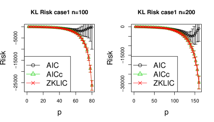
Refer to caption
Figure  3: Comparison between AICAIC\mathrm{AIC}, AICcAICc\mathrm{AICc} and ZKLICZKLIC\mathrm{ZKLIC} under the
          Kullback-Leibler risk in case 1.
Refer to caption
Figure  4: Comparison between AICAIC\mathrm{AIC}, AICcAICc\mathrm{AICc} and ZKLICZKLIC\mathrm{ZKLIC} under the
          Kullback-Leibler risk in case 2.

Figure 5 and Figure 6 show the probability of selecting the true model by each model selection criterion. In Figure 6, the probability of selecting the true model by our model selection criteria is large when the sample size is large. However, in Figure 5, this probability is small; the matrix of regression coefficient has large correlation. Furthermore, the probabilities of selecting the true model by our model selection criteria are smaller than those of existing ones in each case. The reason for this is that the variance of our model selection criteria is bigger than those of the existing ones.
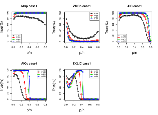
Refer to caption
Figure  5: Comparison between MCp,ZMCp,AIC,AICc,MCpZMCpAICAICc\mathrm{MCp},~{}\mathrm{ZMCp},~{}\mathrm{AIC},~{}\mathrm{AICc}, and ZKLICZKLIC\mathrm{ZKLIC} of
          the probability of selecting the true model in case 1
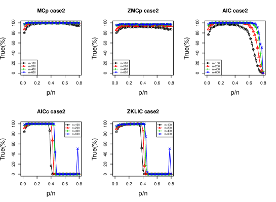
Refer to caption
Figure  6: Comparison between MCp,ZMCp,AIC,AICc,MCpZMCpAICAICc\mathrm{MCp},~{}\mathrm{ZMCp},~{}\mathrm{AIC},~{}\mathrm{AICc}, and ZKLICZKLIC\mathrm{ZKLIC} of
          the probability of selecting the true model in case 2

Although the risks of our model selection criteria are smaller than the ones based on the maximum likelihood estimator, the probability of selecting the true model by our criteria is worse than their probabilities. This is because predictive efficiency and consistency are not compatible (Yang, (2005)) and our criteria are specialized in making the risk smaller.

5 Conclusion

In this paper, we proposed model selection criteria based on the generalized ridge estimator, which improves the maximum likelihood estimator under the squared risk and the Kullback-Leibler risk, in multivariate linear regression. Moreover, we showed that our model selection criteria have the same properties as MCpMCp\mathrm{MCp}, AICAIC\mathrm{AIC}, and AICcAICc\mathrm{AICc} in a high-dimensional asymptotic framework. We demonstrated through the numerical experiments that our model selection criteria have better performances in terms of the risks than the ones based on the maximum likelihood estimators, especially when the matrix of regression coefficients has strong correlation.

Acknowledgement

This work was partially supported by MEXT kakenhi (25730013, 25120012, 26280009, 15H01678 and 15H05707), JST-PRESTO and JST-CREST.

References

  • Akaike, (1971) Akaike, H. (1971). Information theory and an extension of the maximum likelihood principle; 1973. Tsahkadsor, Armenian SSR, pages 267–281.
  • Basser and Pierpaoli, (1998) Basser, P.Β J. and Pierpaoli, C. (1998). A simplified method to measure the diffusion tensor from seven MR images. Magnetic resonance in medicine, 39(6):928–934.
  • Bedrick and Tsai, (1994) Bedrick, E.Β J. and Tsai, C.-L. (1994). Model selection for multivariate regression in small samples. Biometrics, pages 226–231.
  • Davies etΒ al., (2006) Davies, S.Β L., Neath, A.Β A., and Cavanaugh, J.Β E. (2006). Estimation optimality of corrected AIC and modified Cp in linear regression. International statistical review, 74(2):161–168.
  • Fujikoshi etΒ al., (2012) Fujikoshi, Y., Sakurai, T., and Yanagihara, H. (2012). High-dimensional AIC and consistency properties of several criteria in multivariate linear regression. Technical report, TR.
  • Fujikoshi etΒ al., (2014) Fujikoshi, Y., Sakurai, T., and Yanagihara, H. (2014). Consistency of high-dimensional AIC-type and Cp-type criteria in multivariate linear regression. Journal of Multivariate Analysis, 123:184–200.
  • Fujikoshi and Satoh, (1997) Fujikoshi, Y. and Satoh, K. (1997). Modified AIC and Cp in multivariate linear regression. Biometrika, 84(3):707–716.
  • Gharagheizi, (2008) Gharagheizi, F. (2008). Qspr studies for solubility parameter by means of genetic algorithm-based multivariate linear regression and generalized regression neural network. QSAR & Combinatorial Science, 27(2):165–170.
  • Konno, (1991) Konno, Y. (1991). On estimation of a matrix of normal means with unknown covariance matrix. Journal of Multivariate Analysis, 36(1):44–55.
  • Kubokawa and Srivastava, (2001) Kubokawa, T. and Srivastava, M.Β S. (2001). Robust improvement in estimation of a mean matrix in an elliptically contoured distribution. Journal of multivariate analysis, 76(1):138–152.
  • Mallows, (1973) Mallows, C.Β L. (1973). Some comments on Cp. Technometrics, 15(4):661–675.
  • Maruyama and Strawderman, (2005) Maruyama, Y. and Strawderman, W.Β E. (2005). A new class of generalized Bayes minimax ridge regression estimators. The Annals of Statistics, 33(4):1753–1770.
  • Nagai etΒ al., (2012) Nagai, I., Yanagihara, H., Satoh, K., etΒ al. (2012). Optimization of ridge parameters in multivariate generalized ridge regression by plug-in methods. Hiroshima Mathematical Journal, 42(3):301–324.
  • Tsukuma, (2009) Tsukuma, H. (2009). Generalized Bayes minimax estimation of the normal mean matrix with unknown covariance matrix. Journal of Multivariate Analysis, 100(10):2296–2304.
  • Yanagihara and Satoh, (2010) Yanagihara, H. and Satoh, K. (2010). An unbiased Cp criterion for multivariate ridge regression. Journal of Multivariate Analysis, 101(5):1226–1238.
  • Yang, (2005) Yang, Y. (2005). Can the strengths of aic and bic be shared? a conflict between model indentification and regression estimation. Biometrika, 92(4):937–950.