Magneto-hydrodynamical Numerical simulation of wind production from black hole hot accretion flows at very large radii

Abstract

Numerical simulations of black hole hot accretion flows have shown the existence of strong wind. Those works focus only on the region close to black hole thus it is unknown whether or where the wind production stops at large radii. To address this question, Bu et al. (2016) have performed hydrodynamic (HD) simulations by taking into account the gravitational potential of both the black hole and the nuclear star clusters. The latter is assumed to be $\propto\sigma^{2}\ln(r)$, with $\sigma$ being the velocity dispersion of stars and $r$ be the distance from the center of the galaxy. It was found that when the gravity is dominated by nuclear stars, i.e., outside of radius $R_{A}\equiv GM_{\rm BH}/\sigma^{2}$, winds can no longer be produced. That work, however, neglects the magnetic field, which is believed to play a crucial dynamical role in the accretion and thus must be taken into account. In this paper, we revisit this problem by performing magneto-hydrodynamical (MHD) simulations. We confirm the result of Bu et al. (2016), namely wind can’t be produced at the region of $R>R_{A}$. Our result, combined with the results of Yuan et al. (2015), indicates that the formula describing the mass flux of wind $\dot{M}_{\rm wind}=\dot{M}_{\rm BH}(r/20r_{s})$ can only be applied to the region where the black hole potential is dominant. Here $\dot{M}_{\rm BH}$ is the mass accretion rate at the black hole horizon and the value of $R_{A}$ is similar to the Bondi radius.

1. INTRODUCTION

Hot accretion flows are very common in the universe, ranging from low-luminosity active galactic nuclei, which is the majority of nearby galaxies, to the quiescent and hard states of black hole X-ray binaries (see Yuan & Narayan 2014 for a review of our current theoretical understanding of hot accretion flow and its astrophysical applications). One of the most important progresses in our understanding of hot accretion flows in recent years is the finding of strong wind (Yuan et al. 2012b, hereafter YBW12; Narayan et al. 2012; Li et al. 2013; Yuan et al. 2015; Gu 2015). This is an important topic since wind is not only an important ingredient of accretion physics but also plays an important role in AGN feedback (e.g., Ostriker et al. 2010). Because of the mass loss via wind, the mass inflow rate decreases inwards $\dot{M}_{\rm{in}}(r)\propto r^{s}$ with $s\sim 0.5-1$ (see a short review of various numerical simulations in Yuan et al. 2012a). This theoretical prediction was confirmed by the 3 million seconds Chandra observation to the supermassive black hole in our Galactic center, Sgr A* (Wang et al. 2013).

The detailed properties of winds such as the mass flux and terminal velocity are calculated by Yuan et al. (2015). This is achieved by performing trajectory analysis of virtual test particles based on three dimensional general relativistic magneto-hydrodynamic (GRMHD) simulation data. Among others, they find that the mass flux of wind can be described by $\dot{M}_{\rm{wind}}\approx\dot{M}_{\rm{BH}}(r/20r_{s})$, with $\dot{M}_{\rm{BH}}$ is the mass accretion rate at the black hole horizon and $r_{s}$ is the Schwarzschild radius. From this equation, most of the wind comes from the region of large radius. Then a question is how large the value of $r$ can be. To investigate this question, Bu et al. (2016, hereafter Paper I) have performed HD simulations to study the accretion flow at very large radii. We take into account the gravity of both the central black hole and the nuclear star clusters. The velocity dispersion of stars is assumed to be a constant and the gravitational potential of the nuclear star cluster $\propto\sigma^{2}\ln(r)$, where $\sigma$ is the velocity dispersion of stars. We find that there is very few wind launched from the accretion flow in the region where the gravity is dominated by the star cluster.

In Paper I, we introduce an anomalous stress to transfer the angular momentum. In reality, it is the MHD turbulence associated with the magneto-rotational instability (MRI; Balbus & Hawley 1991, 1998) that is responsible for the angular momentum transfer. So MHD simulation is more realistic. Therefore in this paper, we continue our study by performing MHD simulations. As in Paper I, we define a radius $R_{A}$ at which the gravitational force due to the central black hole is equal to that due to the nuclear star cluster. We call $R_{A}$ to be the boundary of the accretion flow or active galactic nuclei (AGNs). This is partly because the value of $R_{A}$ is in reality roughly equal to that of the Bondi radius (Paper I). Hereafter, we use BHAF to refer the hot accretion flow close to the black hole. We use CAAF (circum-AGN accretion flow) to refer the hot accretion flow at larger radii beyond $R_{A}$.

The structure of the paper is as follows. In §2, we describe the basic equations and the set up of the initial conditions. The results of simulations will be given in §3. We discuss and summarize our results in §4.

2. method

2.1. Equations

In a spherical coordinate $(r,\theta,\phi)$, we solve the following magnetohydrodynamical equations describing accretion:

$$\frac{d\rho}{dt}+\rho\nabla\cdot\mathbf{v}=0,$$ (1)

$$\rho\frac{d\mathbf{v}}{dt}=-\nabla p-\rho\nabla\psi+\frac{1}{4\pi}(\nabla\times\mathbf{B})\times\mathbf{B},$$ (2)

$$\rho\frac{d(e/\rho)}{dt}=-p\nabla\cdot\mathbf{v}+\eta\mathbf{J}^{2},$$ (3)

$$\frac{\partial\mathbf{B}}{\partial t}=\nabla\times(\mathbf{v}\times\mathbf{B}-\eta\mathbf{J}).$$ (4)

Here, $\rho$, $p$, $\mathbf{v}$, $\psi$, $e$, $\mathbf{B}$ and $\mathbf{J}(=(c/4\pi)\nabla\times\mathbf{B})$ are density, pressure, velocity , gravitational potential, internal energy, magnetic field and the current density, respectively. $d/dt(\equiv\partial/\partial t+\mathbf{v}\cdot\nabla)$ denotes the Lagrangian time derivative. We adopt an equation of state of ideal gas $p=(\gamma-1)e$, and set $\gamma=5/3$.

The gravitational potential $\psi$ can be expressed as

$$\psi=\psi_{BH}+\psi_{star}.$$ (5)

The black hole potential $\psi_{BH}=-GM_{BH}/(r-r_{s})$, where $G$ is the gravitational constant, $M_{BH}$ is the mass of the black hole and $r_{s}$ is the Schwarzschild radius. As in Paper I, in this paper, we assume that the velocity dispersion of nuclear stars is a constant of radius. This seems to be the case of many AGNs. So the potential of the star cluster is $\psi_{star}=\sigma^{2}\ln(r)+C$, where $\sigma$ is the velocity dispersion of stars and $C$ is a constant. So we have

$$R_{A}=GM_{\rm{BH}}/\sigma^{2}.$$ (6)

We set $\sigma^{2}=10$ and $G=M_{\rm BH}=1$ to define our units in the present work. Under this units we have $R_{A}=0.1$. For a typical physical value of $\sigma\sim(100-400){\rm km~{}s^{-1}}$ (e.g., Kormendy & Ho 2013), $R_{A}\sim(10^{5}-10^{6})r_{s}$. Figure 1 in Paper I shows the gravitational force distribution.

In the above equations, the final terms in Equations (3) and (4) are the magnetic heating and dissipation rate mediated by a finite resistivity $\eta$. The exact form of $\eta$ is same as that used in Stone & Pringle (2001). In the code we adopt, the energy equation is an internal energy equation, numerical reconnection inevitably results in loss of energy from the system. By adding the anomalous resistivity $\eta$, the energy loss can be captured in the form of heating in the current sheet (Stone & Pringle 2001).

In this paper, time is expressed in unit of the orbital time at the torus center.

2.2. Initial conditions

As for the initial condition, we assume a rotating equilibrium torus embedded in a non-rotating, low-density medium. We assume that the torus has constant specific angular momentum $L$ and assume a polytropic equation of state, $p=A\rho^{\gamma}$, where $A$ is a constant. The density distribution of torus is

$$\rho=\rho_{c}\left\{\frac{\max[\Psi(R_{0},\pi/2)-\psi(r,\theta)-L^{2}/(2(r\sin\theta)^{2}),0]}{A[\gamma/(\gamma-1)]}\right\}^{1/(\gamma-1)},$$ (7)

where $R_{0}$ is the density maximum (center) of the torus (Nishikori et al. 2006), $\rho_{c}$ is the density at the torus center. In this paper, we assume $\rho_{c}=1$ and $A=0.4$.

The ambient medium in which the torus is embedded has density $\rho_{0}$ and pressure $\rho_{0}/r$. The mass and pressure of the ambient medius are negligibly small, we choose $\rho_{0}=10^{-4}$.

2.3. Models

The initial magnetic field is generated by a vector potential, i.e. $\mathbf{B}=\nabla\times\mathbf{A}$. In models A1 and A2, the initial magnetic field has a dipolar configuration (same as that in Stone & Pringle 2001). We take $\mathbf{A}$ to be purely azimuthal with $A_{\phi}=\rho^{2}/\beta$, with $\beta=200$. The only difference between models A1 and A2 is that the resolution of model A1 is two times of that of model A2. We find that, the results for models A1 and A2 are almost same. So the resolution in model A2 is enough for our problem. In order to study the dependence of results on initial magnetic field configuration, we carry out model A3. In this model, the initial magnetic field has a quadrapolar configuration with $A_{\phi}=\rho^{2}/\beta r\cos\theta$, and $\beta=100$. Table 1 summarizes the models.

For the initial condition in models A1, A3 and A4, over most of the central regions of the initial torus, we have $6$ grids for one wavelength of the fastest growing mode. Therefore, the fastest growing model of MRI is marginally resolved in our simulations.

In this paper, the simulations are two-dimensional (hereafter 2D). According to the antidynamo theorem (Cowling 1933; Sadowski et al. 2015), the turbulence induced by MRI can not be self-sustaining. Therefore there can not be a true steady state and the quasi-steady state of the simulations is only transient. In this paper, we still preform 2D simulation because on one hand we can simulate a larger radial dynamical range, and on the other hand previous works have indicated that for many problems the results from 2D and 3D simulations are often quite similar (e.g., see the short review in Yuan et al. 2012a in the case of radial profile of inflow and outflow rates). Still, for our present study of wind from accretion flows, it is necessary to carefully examine whether the results from 2D simulation are consistent with those from 3D simulation.

In order to answer this question, we have carried out a 2D MHD simulation of accretion flows close to a black hole. The domain of the simulation is $2r_{s}$-$400r_{s}$. In this simulation, only the black hole gravity is taken into account. Using the trajectory approach as described in Yuan et al. (2015), we have calculated the mass flux of wind, which is $\sim 52\%$ of the total outflow rate calculated by Equation (9). As comparison, the mass flux of wind calculated in Yuan et al. (2015), which is based on 3D MHD simulation data of accretion flow, is $\sim 60\%$ of the total outflow rate calculated by Equation (9). Such a good consistency suggests that the present 2D study should be a good approximation.

Table 1models in this paper

Models	Initial magnetic field	Resolution	Computational domain
A1	dipolar	$294\times 160$	0.03-4
A2	dipolar	$147\times 80$	0.03-4
A3	quadrapolar	$294\times 160$	0.02-4
A4	dipolar	$294\times 160$	0.002-0.4

2.4. Numerical Method

We use the ZEUS-2D code (Stone & Norman 1992a, 1992b) to solve Equations (1)-(4). The polar range is $0\leq\theta\leq\pi$. We adopt non-uniform grid in the radial direction $(\bigtriangleup r)_{i+1}/(\bigtriangleup r)_{i}=1.037$. The distributions of grids in $\theta$ direction in the northern and southern hemispheres are symmetric about the equatorial plane. The resolution at $\theta$ in the northern hemisphere is same as that at $\pi-\theta$ in the southern hemisphere. In order to well resolve the accretion disk around the equatorial plane, the resolution is increased from the north and south rotational axis to the equatorial plane with $(\bigtriangleup\theta)_{j+1}/(\bigtriangleup\theta)_{j}=0.9826$ for $0\leq\theta\leq\pi/2$ and $(\bigtriangleup\theta)_{j+1}/(\bigtriangleup\theta)_{j}=1.0177$ for $\pi/2\leq\theta\leq\pi$. At the poles, we use axisymmetric boundary conditions. At the inner and outer radial boundary, we use outflow boundary conditions.

3. RESULTS

3.1. Mass inflow rate

Following Stone et al. (1999), we define the mass inflow and outflow rates, $\dot{M}_{in}$ and $\dot{M}_{out}$ as follows,

$$\dot{M}_{\rm in}(r)=2\pi r^{2}\int_{0}^{\pi}\rho\min(v_{r},0)\sin\theta d\theta,$$ (8)

$$\dot{M}_{\rm out}(r)=2\pi r^{2}\int_{0}^{\pi}\rho\max(v_{r},0)\sin\theta d\theta.$$ (9)

The net mass accretion rate is,

$$\dot{M}_{\rm acc}(r)=\dot{M}_{\rm in}(r)+\dot{M}_{\rm out}(r).$$ (10)

Note that the above rates are obtained by time-averaging the integrals rather than integrating the time averages.

Figure 1 shows the time-averaged (from 130-136 orbits) and angle-integrated mass rates of model A1. Both the mass inflow and outflow rates decrease inward. This is consistent with that found in the HD simulations in Paper I. We note that the mass inflow and outflow rates are not good power-law function of radius, just like the case of a BHAF (Stone & Pringle 2001). This is likely because the radial distribution of the strength of magnetic field is not very smooth. Because of the accumulation of magnetic flux during the simulation, the magnetic field in the inner region of the accretion flow is much stronger than the other region. We will see in §3.4 that, in model A3 there is no such accumulation of magnetic flux due to the initial quadrapolar configuration, the radial profiles become smoother.

To reach a steady state at a certain radius, the simulation time should be at least equal to the accretion timescale at that radius. According to this criterion, our simulation of model A1 has reached a steady state within $r\sim 0.6$. We note that the flow in model A1 is convectively unstable (see section 3.3). The accretion timescale is roughly equal to one turnover time of local convective eddies. It may require many turnover times for the convection to reach a steady state. Thus it will be interesting to run our simulations for several times longer in the future to check whether the results will change.

Figure 1.— The radial profile of the time-averaged (from $t=130$ to 136 orbits) and angle integrated mass inflow rate $\dot{M}_{\rm in}$ (solid line), outflow rate $\dot{M}_{\rm out}$ (dashed line), and the net rate $\dot{M}_{\rm acc}$ (dotted line) in model A1. They are defined in Equations (8), (9), and (10), respectively.

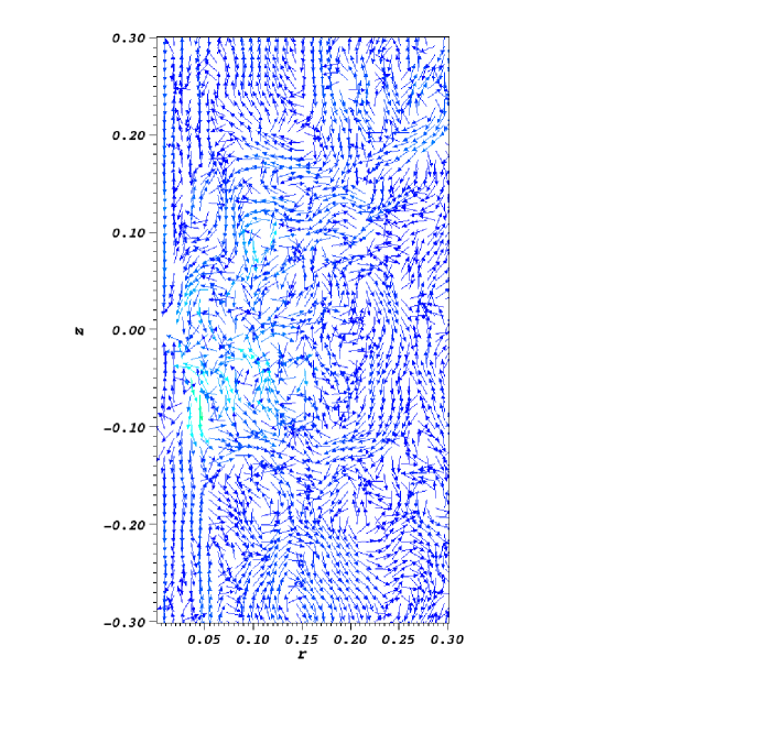
Figure 2.— Snapshot of velocity vector of model A1 at $t=130$ orbits. Clearly, turbulent eddies occupy the whole domain and it is hard to find winds.

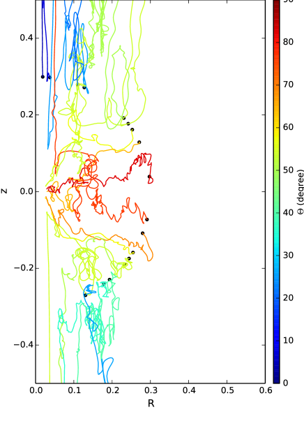
Figure 3.— Trajectory of gas for model A1. The black dots located at $r=0.3$ are starting points of the “test particle”. Different colors denote trajectory of “test particle” starting from different $\theta$ angle. It is clear that the “test particle” crosses the starting radius for many times. From this figure we can see that the real wind trajectories, i.e., the trajectories which extend from $r=0.3$ to large radius and never come across $r=0.3$ again are very few. Winds are very weak.

3.2. Does strong wind exist in a CAAF ?

The significant mass outflow rate shown in Figure 1 does not mean the existence of strong real outflow (wind) because it may be due to the turbulent motion. To study whether wind exists, let us first directly look at the velocity field shown in Figure 2. We see that turbulent eddies occupy the whole domain and it is hard to find systematic winds.

To investigate this problem precisely, following Yuan et al. (2015), we use the trajectory method to study the motion of the virtual particles. The details of this approach can be found in Yuan et al. (2015). To get the trajectory, we first need to choose some virtual “test particle” in the simulation domain. They are of course not real particles, but some grids representing fluid elements. Their locations and velocities at a certain time $t$ are obtained directly from the simulation data. We can then obtain their location at time $t+\delta t$ from the velocity vector and $\delta t$. Trajectory is more loyal than streamline to reflect the motion of particles which is crucial for us to investigate whether real wind exists. Trajectory is only equivalent to the streamline for strictly steady motion, which is not the case for accretion flow since it is always turbulent.

Trajectory approach can easily tell us which particles are real outflows (i.e., winds) and which are doing turbulent motions. Combining with the density and velocity field information from the simulation data we can then obtain the various properties of wind such as the mass flux, angular distribution, and velocity (see Yuan et al. 2015 for details). Figure 3 shows the trajectory of some gas particles starting from $r=0.3$ in model A1. From this figure we can see that the real wind trajectories, i.e., the trajectories which extend from $r=0.3$ to large radius and never come across $r=0.3$ again, are very few. This implies that the mass flux of wind is very small. Our quantitative calculation confirms this result. For example, we find at $r=0.4$ the ratio of mass flux of winds to the total outflow rate calculated by Equation (9) is only $0.2\%$. This result means that there is almost no wind. This result is consistent with that found in Paper I. As a comparison, in the case of BHAF, Yuan et al. (2015) find that this ratio is $60\%$.

3.3. Why the inflow rate decreases inward in a CAAF?

If wind is absent, what is the reason for the inward decrease of inflow rate? To answer this question, we need to examine the convective stability of the accretion flow. Hydrodynamical simulation of BHAFs (e.g., Stone et al. 1999; Igumenshchev & Abramowicz 1999, 2000; Yuan & Bu 2010) have found that the flows are convectively unstable, consistent with what has been suggested by the one-dimensional analytical study of BHAFs (Narayan & Yi 1994). The physical reason is that the entropy of the flow increases inward, which is resulted by the viscous heating and negligible radiative loss. However, in the presence of magnetic field, numerical simulations have found that a BHAF becomes convectively stable (Narayan et al. 2012; YBW12). In the case of a CAAF, Paper I has found that the flow is convectively unstable, same as the case of a BHAF.

We now study whether a CAAF is convectively stable or not in the presence of magnetic field. We use the Høiland criteria (e.g., Tassoul 1978; Begelman & Meier 1982):

$$(\nabla s\cdot\mathbf{dr})(\mathbf{g}\cdot\mathbf{dr})-\frac{2\gamma v_{\phi}}{R^{2}}[\nabla(v_{\phi}R)\cdot\mathbf{dr}]dR<0.$$ (11)

In Equation (11), $R=r\sin\theta$ is the cylindrical radius, ${\bf dr}=dr\hat{r}+rd\theta\hat{\theta}$ is the displacement vector, $s=\ln(p)-\gamma\ln(\rho)$ is $(\gamma-1)$ times the entropy, ${\bf g}=-\nabla\psi+\hat{R}v_{\phi}^{2}/R$ is the effective gravity, and $v_{\phi}$ is the rotational velocities. For a non-rotating flow, this condition is equivalent to an inward increase of entropy, which is the well-known Schwarzschild criteria.

Taking model A1 as an example, Figure 4 shows the result. The result is obtained according to Equation (11) based on the simulation data at t=132 orbits at the initial torus center $r=1$. At $t=132$ orbits, the flow has achieved a steady state since the net accretion rate averaged between $t=130$ to 136 orbits is a constant of radius (see figure 1, the dotted line). The red regions are convectively unstable. We can see from the figure that a CAAF is mostly convectively unstable. This is different from the case of a BHAF with magnetic field. The reason should be due to the change of the gravitational potential but the detail remains unclear. This result strongly implies that the inward decrease of inflow rate is because of convection and it reminds us the scenario of convection-dominated accretion flow (CDAF) proposed by Narayan et al. (2000) and Quauaert & Gruzinov (2000), although that model was proposed to explain the dynamics of BHAFs rather than CAAFs.

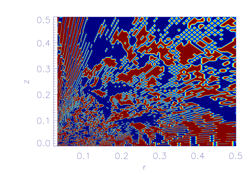
Figure 4.— Convective stability analysis of Model A1. The result is obtained according to Equation (11) based on the simulation data at t=132 orbits at the initial torus center $r=1$. The red region is unstable.

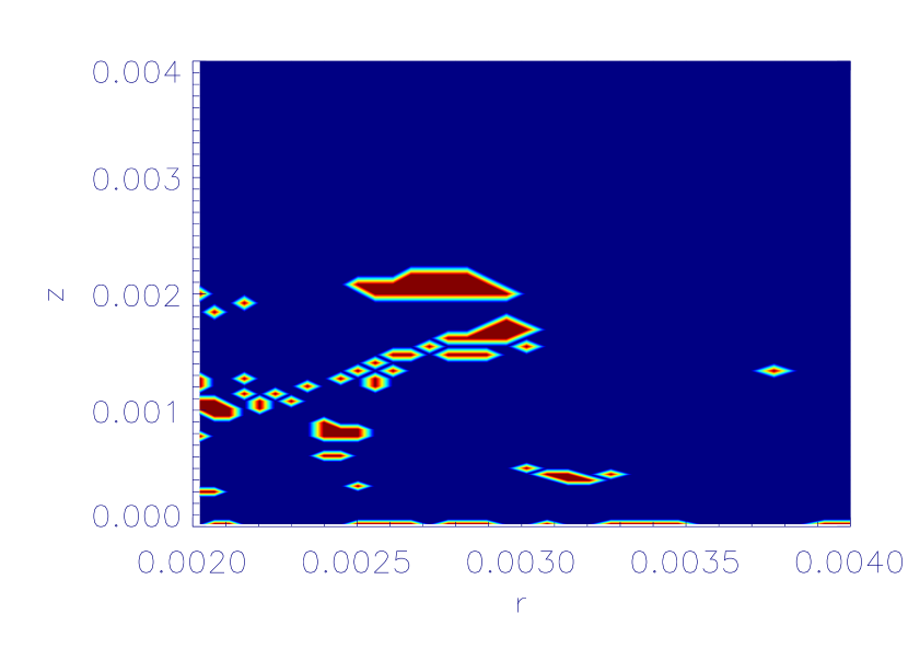
Figure 5.— Convective stability analysis of Model A4. The result is obtained according to Equation (11) based on the simulation data at t=100 orbits at the initial torus center $r=0.1$. The red region is unstable.

From Figure 4, it seems that the region $r<0.1$ is convectively unstable. Our previous work with only black hole gravity does show that the flow is convectively stable (YBW12). We think the apparent discrepancy is because of the contamination of the gravitational potential by the star cluster. In model A1, in the region $r<0.1$, it is true that the black hole gravity is bigger than that of the star cluster, but the gravity of the stars is not negligible. In fact, in the region $0.03<r<0.1$, the black hole gravity is bigger than that of star cluster at most by a factor of 4. To further investigate this point, we have analyzed the convective stability of model A4. Figure 5 shows the results of the region very close to the black hole where the black hole gravity is strongly dominant. We can clearly see that the flow is convectively stable.

3.4. Varying the initial configuration of magnetic field

Figure 6.— Same as Figure 1, but for model A3. The time-average is taken from $t=127$ to 130 orbits.

In order to study whether the results depend on the initial configuration of the magnetic field, we carry out model A3. In this model, the initial configuration of magnetic field is quadrapolar. Figure 6 shows the inflow, outflow, and net rates. The inflow rate is smoother than that in Figure 1, as we have explained in §3.1. In addition to that, we find that all results are almost same with those of model A1, namely the flow is convectively unstable, and wind is absent. Quantitatively, using the trajectory method, we find at $r=0.4$ , the ratio of mass flux of winds to the total outflow rate calculated by Equation (9) is $0.1\%$.

3.5. Moving the computational domain inward

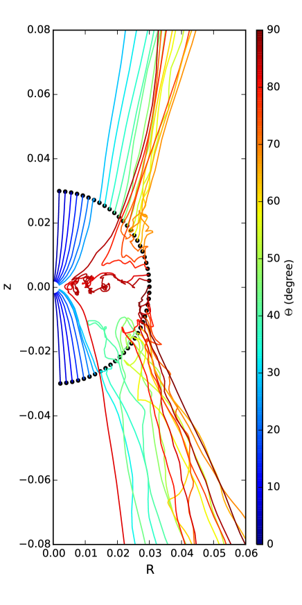
Figure 7.— Trajectory of gas for model A4. The black dots located at $r=0.03$ are starting points of the “test particle”. Different colors denote trajectory of “test particle” starting from different $\theta$ angle. It is clear that wind is present when the black gravity dominates.

From Figures 1 and 6, in the region $r<0.1$, the outflow rate is very small. This region is dominated by the gravity of black hole. Previous works (Yuan et al. 2012b; Yuan et al. 2015) have shown that in this case outflow (wind) should be strong. The apparent discrepancy between this work and our previous works is due to the fact that the region $r<0.1$ is too close to the inner boundary where a somewhat “unphysical” boundary condition (i.e., outflow condition) is adopted. This condition means that the gas entering into the inner boundary is assumed to disappear and the gradient of physical variables at the boundary is zero. However, in reality, there should be some flow entering into the inner boundary and the flows inside and outside of the boundary can interact with each other. This will significantly affect the properties of the flows around the inner boundary.

In order to illustrate this point, we have carried out model A4. In this model, our computational domain is $0.002<r<0.4$. The gravitational potential from both the black hole and the nuclear star cluster are included but obviously the former dominates. The initial condition of the magnetic field is dipolar. Figure 7 shows the trajectory of some gas particles starting from $r=0.03$. From this figure, it is clear that strong wind is present in this case. Combined with the results presented in previous sections, this result indicates that the disappearance of wind is because of the changes of the gravitational potential.

In models A1 and A4, the setup of the model, the equations, and the potential formula we use are exactly same. The only difference between them is that the black hole potential is more dominates in A4 while the stellar cluster potential is more dominates in A1. Therefore, the disappearance of wind is because of the changes of the gravitational potential.

4. CONCLUSION AND DISCUSSION

Numerical simulations show that strong winds exist in black hole hot accretion flow (e.g., YBW12). The mass flux of wind follows $\dot{M}_{\rm wind}=\dot{M}_{\rm BH}(r/20r_{s})$ (Yuan et al. 2015). A question is then what the value of $r$ can be, i.e., whether or where the wind production stops. In order to answer this question, in Paper I, we have performed HD simulations and take into account the gravity of both the black hole and nuclear stars cluster. We find that the mass inflow rate decreases inward. However, our trajectory analysis indicates that there is no wind when the potential of star cluster dominates, i.e., beyond a certain radius $R_{A}\equiv GM_{\rm BH}/\sigma^{2}$, with $\sigma$ being the velocity dispersion of stars. The inward decrease of inflow rate is not because of strong wind, as in the case of accretion flow in which the black hole potential dominates, but because of the convective instability of the accretion flow. In this paper, we revisit the same problem by performing more realistic MHD simulations. We find again that the conclusion remains unchanged, i.e., there is no wind beyond $R_{A}$. Our stability analysis again indicates that the MHD accretion flow beyond $R_{A}$ is convectively unstable. This is different from the case of accretion flow when the black hole potential dominates (YBW12; Narayan et al. 2012). So the inward decrease of inflow rate is likely because of the convective motion of the flow.

This result indicates that the mass flux of wind found by Yuan et al. (2015):

$$\dot{M}_{\rm wind}=\dot{M}_{\rm BH}(r/20r_{s}),$$ (12)

can only be applied to the region where the black hole gravitational force dominates. In the star cluster potential dominates region, i.e., beyond $R_{A}$, no wind will be produced. In practice, the value of $R_{A}$ is close to the Bondi radius $R_{B}\equiv GM_{\rm BH}/c_{s}^{2}$ (Paper I).

What is the reason for the absence of wind beyond $R_{A}$? We speculate that it may be related with the change of the slope of the gravitational potential. Such a change would change the shear of the accretion flow and then the turbulent stress in the accretion flow. Analytical models of accretion disk (e.g., Shakura & Sunyaev 1973) usually assume that viscous stress is proportional to the shear of the accretion disk,

$$T_{r\phi}=\rho\nu r\frac{d\Omega}{dr}$$ (13)

with $\nu=\alpha c_{s}^{2}/\Omega_{k}$. $c_{s}$, $\Omega$ and $\Omega_{k}$ are sound speed, angular velocity and Keplerian angular velocity, respectively. Recent 3D MHD numerical simulations show that the turbulent stress is not linearly proportional to the shear, but the dependence is stronger than that predicted by Equation (13) (Pessah et al. 2008; Penna et al. 2013). This implies that the change of the potential changes some properties of turbulence which then change the wind production.

References

- (1) Balbus S. A., Hawley J. F., 1991, ApJ, 376, 214
- (2) Balbus S. A., Hawley J. F., 1998, Rev. Mod. Phys., 70,1
- (3) Bu D. F., Yuan F., Gan Z. M., Yang X. H., 2016, ApJ, 818, 83
- (4) Begelman, M. C. & Meier, D. L. 1982, ApJ, 253, 873
- (5) Cowling T. G. 1933, MNRAS, 94, 39
- (6) Gu W. M., 2015, ApJ, 799, 71
- (7) Igumenshchev I. V., Abramowicz M. A., 1999, MNRAS, 303, 309
- (8) Igumenshchev I. V., Abramowicz M. A., 2000, ApJS, 130, 463
- (9) Kormendy J., Ho L. C., 2013, ARA&A, 51, 511
- (10) Li J., Ostriker J., Sunyaev R., 2013, ApJ, 767,105
- (11) Narayan R., Yi I., 1994, ApJ, 428, L13
- (12) Narayan R., Igumenshchev I. V., Abramowicz M. A., 2000, ApJ, 539, 798
- (13) Narayan R., Sadowski A., Penna R. F., Kulkarni A. K., 2012, MNRAS, 426, 3241
- (14) Nishikori H., Machida M., Matsumoto R., 2006, ApJ, 641, 862
- (15) Ostriker J. P., Choi E., Ciotti L., Novak G. S., Proga D., 2010, ApJ, 722, 642
- (16) Pessah M. E., Chan C. K., Psaltis D., 2008, MNRAS, 383, 683
- (17) Penna R. F., Sadowski A., Kulkarni, A. K., Narayan R., 2013, MNRAS, 428, 2255
- (18) Quataert E., Gruzinov A., 2000, ApJ, 539, 809
- (19) Sadowski A., Narayan R., Tchekhovskoy A., Abarca D., Zhu Y., McKinney J. C., 2015, MNRAS, 447, 49
- (20) Shakura N. I., Sunyaev R. A., 1973, A&A, 24, 337
- (21) Stone J. M., Norman M. L., 1992a, ApJS, 80, 753
- (22) Stone J. M., Norman M. L., 1992b, ApJS, 80, 791
- (23) Stone J. M., & Pringle J. E., 2001, MNRAS, 322, 461
- (24) Stone J. M., Pringle J. E., & Begelman M. C. 1999, MNRAS, 310, 1002
- (25) Tassoul, J.-L. 1978, Theory of Rotating Stars (Princeton: Princeton Univ. Press)
- (26) Wang Q. D., Nowak M. A., Markoff S. B., et al. 2013, Sci, 341, 981
- (27) Yuan F., Bu D., 2010, MNRAS, 408, 1051
- (28) Yuan F., Bu D., Wu M., 2012b, ApJ, 761, 130
- (29) Yuan F., Wu M., Bu D., 2012a, ApJ, 761, 129
- (30) Yuan F., Gan Z. M., Narayan R., Sadowski A., Bu D. F., Bai X. N., 2015, ApJ, 804, 101
- (31) Yuan F., Narayan R., 2014, ARA&A, 52, 529