Stern-Gerlach splitters for lattice quasispin

Abstract

We design a Stern-Gerlach apparatus that separates quasispin components on the lattice, without the use of external fields. The effect is engineered using intrinsic parameters, such as hopping amplitudes and on-site potentials. A theoretical description of the apparatus relying on a generalized Foldy-Wouthuysen transformation beyond Dirac points is given. Our results are verified numerically by means of wave-packet evolution, including an analysis of Zitterbewegung on the lattice. The necessary tools for microwave realizations, such as complex hopping amplitudes and chiral effects, are simulated.

I Introduction

Quantum emulations have been increasingly important for theorists and experimentalists in areas such as ultracold atoms Morsch and Oberthaler (2006); Bloch (2005); Oberthaler et al. (1996); Uehlinger et al. (2013); Struck et al. (2012), quantum and microwave billiards Kuhl et al. (2010); Barkhofen et al. (2013); Bittner et al. (2010); Bellec et al. (2013), plasmonic circuits Martínez-Galera et al. (2014), and artificial solids in general Polini et al. (2013); Gomes et al. (2012). The concept can be used to engineer quantum dynamics not readily accessible in naturally occurring physical systems, e.g., elementary particles or charge carriers in solids Semenoff (1984); Geim and Novoselov (2007). For some years, the effective Dirac theories emerging in honeycomb lattices and linear chains Neto et al. (2009); Roati et al. (2007); Fallani et al. (2007); Franco-Villafañe et al. (2013); Sadurní et al. (2013, 2010) have led researchers to consider the use of quasispin as an internal degree of freedom capable of supporting the long-pursued realization of qubits in solid-state physics. This interesting degree of freedom has the property of being nonlocal, inherent to the crystalline structure, and sufficiently robust as to provide upper and lower bands around conical (Dirac) points in the spectrum. In the same context, there has been a recent interest in Majorana fermions Mancini et al. (2015); Wilczek (2009); Alicea (2012), as their topological nature may provide robustness with respect to decoherence, hence increasing the life of qubits, and thus extending the reach of potential applications. Several theoretical developments take advantage of quasispin Kagalovsky et al. (1999); Bernard and LeClair (2001) and some experiments in lattices have observed their effects, e.g., Zitterbewegung in photonic structures Dreisow et al. (2010).

But how does one measure quasispin on the lattice? One of the goals of this paper is to gain access to this degree of freedom by designing an interaction on bipartite lattices with the following features: (a) an adjustable coupling with particles’ quasispin, (b) a localized region where the interaction occurs, and (c) an intrinsic generation of the interaction using lattice parameters. It is worth mentioning that the electron’s true spin is not easily accessible when immersed in a solid Meier et al. (2007).

Our tasks demand an exploration of tight-binding models, oriented to an experimental setup in microwave resonators. We establish the realization of Dirac’s equation in a one-dimensional setting and solve the problem of how to split the two components of the wave function, namely particle-antiparticle components, or, in the language of solid-state physics, the upper and lower bands. Under these circumstances, and using the Foldy-Wouthuysen (FW) transformation, we design and test a spatially localized Stern-Gerlach splitter represented by a banded matrix, to be used in the context of Dirac-like dynamics. In this case, the experimental restrictions imposed by most realizations come in the form of short-range interactions. We provide a successful geometric proposal in compliance with such restrictions, using microwave resonators coupled by proximity.

We approach the problem in three different stages. First, in Sec. II, we study the lattice structure using full-band Dirac equations Sadurní et al. (2010) and provide a generalized FW transformation in Sec. II.1. The explicit construction of the beam splitter as a potential is achieved in Sec. II.2. In Sec. III, we study wave-packet dynamics using numerical simulations with two important results: in Sec. III.1, we show that unpolarized beams exhibit Zitterbewegung, while in Secs. III.2 and III.3, we test the splitter efficiency. With the aim of ensuring the feasibility of our model, in Sec. IV we establish the robustness of the system under random perturbations of parameters. Our study is applicable to any tight-binding (TB) array with the aforementioned structure, but, as a final step, in Sec. V we focus on plausible experiments in microwave cavities. Section V.1 describes the necessary specifications for the implementation and Sec. V.2 gives an explicit construction that produces negative couplings and level inversion. We conclude in Sec. VI.

II Intrinsic Stern-Gerlach apparatus

II.1 Quasispin and generalized FW transformations

Figure 1: A visualization of the FW transformation. Using a rotation around the $z$ axis by an angle $\phi$, followed by a rotation around $y$ by an angle $\theta$, would rotate the eigenstates of $\sigma_{z}$ to the eigenstates of the Hamiltonian given by Eq. (1). In this visualization, the angles are considered to be scalars since they are operators that commute with the Hamiltonian.

Let us define our periodic system, with the aim of generalizing the usual FW unitary rotation Foldy and Wouthuysen (1950); Vries (1970). Consider a one-dimensional lattice, with sites characterized by the positions $n\in\mathbb{Z}$, and position basis $\{|n\rangle\}_{n\in\mathbb{Z}}$. We deal with a typical TB model in this setting, with hopping parameter $\Delta$ and potential $V$,

$$H =\Delta T+\Delta T^{\dagger}+V$$

$$=\sum_{n=-\infty}^{\infty}\Delta|n\rangle\langle n+1|+\mbox{h.c.}+V_{n}|n\rangle\langle n|$$ (1)

where the translation operator is defined via $T|n\rangle=|n+1\rangle$ and a position-dependent potential $V=\sum_{n}V_{n}|n\rangle\langle n|$ has been introduced. We have shown Sadurní et al. (2010) that this Hamiltonian can be written in Dirac form without approximations, with suitable definitions of Dirac matrices $\alpha$ in terms of projectors onto even and odd site numbers,

$$H=\Delta\mbox{\boldmath$\alpha$\unboldmath}\cdot{\bf\Pi}+V$$ (2)

with the kinetic operators

$$\Pi_{1} \equiv 1+\frac{1}{2}\sum_{n}|n-2\rangle\langle n|+|n\rangle\langle n-2|=1+\frac{T^{2}+(T^{\dagger})^{2}}{2}$$

$$\Pi_{2} \equiv\frac{i}{2}\sum_{n}|n-2\rangle\langle n|-|n\rangle\langle n-2|=\frac{T^{2}-(T^{\dagger})^{2}}{2i}$$ (3)

and the Dirac matrices

$$\alpha_{1}\equiv\sum_{n\,\mbox{\scriptsize even}}|n+1\rangle\langle n|+|n\rangle\langle n+1|$$

$$\alpha_{2}\equiv i\sum_{n\,\mbox{\scriptsize even}}|n+1\rangle\langle n|-|n\rangle\langle n+1|$$ (4)

satisfying the usual conditions, as proved in Sadurní et al. (2010).

Bipartite lattices with alternating on-site potential energies $E_{1}$, $E_{2}$ entail the use of the potential

$$V=E_{0}+\mu\beta,$$ (5)

where the average energy $E_{0}=(E_{1}+E_{2})/2$ and splitting $\mu=(E_{1}-E_{2})/2$ are used. Additionally, we have considered the operator $\beta$, here defined as

$$\beta\equiv\sum_{n\,\mbox{\scriptsize even}}|n\rangle\langle n|-|n+1\rangle\langle n+1|.$$ (6)

Our lattice operators (4) and (6) satisfy the relations $\left\{\alpha_{i},\beta\right\}=0,\left\{\alpha_{i},\alpha_{j}\right\}=2\delta_{ij},\left[\alpha_{1},\alpha_{2}\right]=2i\beta$. This reordering of our original TB Hamiltonian leads to an effective Dirac Hamiltonian of the form

$$H=\Delta\mbox{\boldmath$\alpha$\unboldmath}\cdot{\bf\Pi}+\mu\beta+E_{0}.$$ (7)

The spectrum of $H$ is $E_{k,\pm}=E_{0}\pm\sqrt{4\Delta^{2}\cos^{2}k+\mu^{2}}\equiv E_{0}\pm E_{k}$ and, most importantly, its eigenfunctions are written as spinors with up and down components represented by amplitudes in the even and odd sublattices. Here we remark that this spinorial form of the eigenfunctions and, in general, of any wave packet on the lattice is in itself an additional discrete degree of freedom, and thus gives rise to the name: quasispin. As previously noted, quasispin is entirely nonlocal, given that it is a direct manifestation of the bipartite nature of the lattice.
Returning to the discussion, we have the following complete set of eigenfunctions

$$\langle n|k,s\rangle=e^{ikn}\left(\begin{array}[]{c}u^{+}_{k,s}\\ u^{-}_{k,s}\end{array}\right),\,u^{\pm}_{k,s}=s^{\pm 1/2}\sqrt{\frac{E_{k}\pm s\mu}{4\pi E_{k}}},$$ (8)

where $n$ is an even index, $k$ is the wave number in the reduced Brillouin zone $0<k<\pi$, and $s=\pm$ is the index of upper and lower bands. For the latter use, we introduce the parameter $\kappa$ around the conical point $k=\pi/2-\kappa/2$. This yields the following eigenvalues $p_{i}$ of $\Pi_{i}$:

$$p_{1}\approx-\frac{\kappa^{2}}{2},\qquad p_{2}\approx\kappa$$ (9)

for momenta near the conical point. This shows that $p_{2}$ survives, playing the role of an effective momentum of a one-dimensional (1D) Dirac equation.

In order to show the role of quasispin in the solutions, one can solve the eigenvalue problem without any approximation by means of a rotation in the space $(\alpha_{1},\alpha_{2},\beta)$. This is the FW transformation explained in Fig. 1, which maps the site model (even/odd sites) to a qubit system of positive and negative energies Sadurní et al. (2013, 2010). In terms of Pauli matrices, we write $\alpha_{1}=\sigma_{1},\alpha_{2}=\sigma_{2},\beta=\sigma_{3}$ and we define a vector ${\bf v}$ with components $v_{1}=\Delta\Pi_{1},v_{2}=\Delta\Pi_{2},v_{3}=\mu$. With these definitions, $H$ becomes a pure spin-orbit interaction,

$$H-E_{0}={\bf v}\cdot\mbox{\boldmath$\sigma$\unboldmath},\qquad\left[v_{i},v_{j}\right]=\left[v_{i},\sigma_{j}\right]=0.$$ (10)

This allows one to rotate the vector ${\bf v}$ independently of $\sigma$, with the aim of making it parallel to ${\bf z}$. Equivalently, the rotation is represented by a unitary transformation $U_{\mbox{\scriptsize FW}}$ which block diagonalizes $H$,

$$U_{\mbox{\scriptsize FW}}=\exp\left(-\frac{i\phi}{2}\sigma_{3}\right)\exp\left(-\frac{i\theta}{2}\sigma_{2}\right)$$ (11)

In our case, this rotation allows us to guide the design of the polarizer. The exponential is understood in terms of trigonometric functions, where the angles are operators defined by

$$\sin\theta =\frac{\Delta(T+T^{\dagger})}{\sqrt{\Delta^{2}(T+T^{\dagger})^{2}+\mu^{2}}},$$

$$\cos\theta =\frac{\mu}{\sqrt{\Delta^{2}(T+T^{\dagger})^{2}+\mu^{2}}}$$ (12)

and

$$\cos\phi=\frac{1}{2}(T+T^{\dagger}),\quad\sin\phi=\frac{1}{2i}(T-T^{\dagger}).$$ (13)

Formula (11) involves trigonometric functions of half angles, so we provide their expressions for completeness [we note here that $(H-E_{0})^{2}$ is independent of Pauli matrices],

$$\cos\left(\frac{\theta}{2}\right) =\sqrt{\frac{\sqrt{(H-E_{0})^{2}}+\mu}{2\sqrt{(H-E_{0})^{2}}}},$$

$$\sin\left(\frac{\theta}{2}\right) =\sqrt{\frac{\sqrt{(H-E_{0})^{2}}-\mu}{2\sqrt{(H-E_{0})^{2}}}},$$ (14)

and

$$\cos\left(\frac{\phi}{2}\right) =\frac{1}{2}(T^{1/2}+(T^{\dagger})^{1/2}),$$

$$\sin\left(\frac{\phi}{2}\right) =\frac{1}{2i}(T^{1/2}-(T^{\dagger})^{1/2}).$$ (15)

With the unitary operator $U_{\mbox{\scriptsize FW}}$, the transformation yields, in a very clean way,

$$H_{\mbox{\scriptsize FW}} =U_{\mbox{\scriptsize FW}}^{\dagger}HU_{\mbox{\scriptsize FW}}$$

$$=\begin{pmatrix}E_{0}+\sqrt{(H-E_{0})^{2}}&0\\ 0&E_{0}-\sqrt{(H-E_{0})^{2}}\end{pmatrix}$$

where $\sqrt{(H-E_{0})^{2}}=\sqrt{\Delta^{2}(T+T^{\dagger})^{2}+\mu^{2}}$.

Adding the next-to-nearest-neighbor interaction in Eq.  (1) would require a modification of the definitions (3). However, the program of the present section could also be carried out in a very similar fashion. The addition of the quartic translational terms in Eq. (3) would change Eqs. (12) and (13), and would thus make the propagation in the two bands slightly different. A splitter could thus also be designed, but an asymmetry in the two components would indeed show up in the asymptotic evolution.

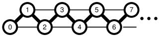
Figure 2: Lattice topologies corresponding to the polarizer, up to second neighbors (top) and third neighbors (bottom). Thick lines correspond to the (strongest) nearest-neighbor interaction, thin lines are the next-to-nearest-neighbor interactions, and, finally, dashed lines are the weakest (and in the top model neglected) third-nearest-neighbor interactions.

II.2 The Stern-Gerlach apparatus as an interaction

Now that we have derived a block-diagonal Hamiltonian, we are in the position to introduce an interaction which couples differently with positive- and negative-energy solutions. Moreover, we shall see that the range of such interaction can be controlled at pleasure. A diagram is shown in Fig. 2.

In classical relativistic dynamics, the double sign of the kinetic energy could be used to produce two types of behavior in the presence of a potential well. If $V(x)$ interacts attractively for positive solutions (charges), the opposite case will be a potential barrier acting on negative solutions (holes):

$$E=\pm\sqrt{c^{2}p^{2}+m^{2}c^{4}}+V(x).$$ (16)

Thus, one type of solution would be allowed to enter in a certain region while the other would be rejected; we may regard $V(x)$ as a gate keeper. We must note, however, that quantum dynamics gives rise to interference phenomena producing transmission and reflection in both of the aforementioned situations. The simplest way to separate both types of waves is by introducing a potential of the type

$$V_{\pm}(x)=\begin{cases}V(x)&\text{for particles}\\ 0&\text{for holes}\end{cases}$$ (17)

Since the FW transformation does the job of decoupling both types of solutions, we introduce at the level of $H_{\mbox{\scriptsize FW}}$ a potential $V_{\mbox{\scriptsize FW}}$ that separates the components as in (17),

$$\tilde{H}_{\mbox{\scriptsize FW}}=H_{\mbox{\scriptsize FW}}+\frac{{\bf 1}+\sigma_{3}}{2}\otimes V_{\mbox{\scriptsize FW}}$$ (18)

or in matrix form,

$$\begin{pmatrix}E_{0}+V_{\mbox{\scriptsize FW}}+\sqrt{(H-E_{0})^{2}}&0\\ 0&E_{0}-\sqrt{(H-E_{0})^{2}}\end{pmatrix}.$$

In order to find the true potential $V$ operating at the level of lattice sites and neighbor couplings, we must return to our original description by means of the inverse FW transformation,

$$V(N)=U_{\mbox{\scriptsize FW}}\,V_{\mbox{\scriptsize FW}}\,U^{\dagger}_{\mbox{\scriptsize FW}}.$$ (19)

Direct computations lead to a $2\times 2$ block form of $V$. For instance,

$$V_{11}=e^{-i\phi/2}\cos\left(\frac{\theta}{2}\right)V_{\mbox{\scriptsize FW}}\cos\left(\frac{\theta}{2}\right)e^{i\phi/2}$$ (20)

Here we may choose $V_{\mbox{\scriptsize FW}}$ at will, but using site number kets makes it easier to provide locality: $\langle n|V_{\mbox{\scriptsize FW}}|n^{\prime}\rangle=\delta_{n,n^{\prime}}V_{\mbox{\scriptsize FW}}(n)$. The site dependence of $V$ can be obtained by inserting a complete set of Bloch waves. Let us define

$$I_{n}^{s,s^{\prime}}\left(\frac{\mu}{\Delta}\right)\equiv\int_{-\pi}^{\pi}dk\sqrt{\frac{E_{k}+s\mu}{E_{k}}}\,e^{ik(n-s^{\prime}/2)},$$ (21)

with $s,s^{\prime}=\pm$ and $n\in\mathbf{Z}$. The potential blocks are then

$$\langle n|V_{11}|n^{\prime}\rangle=\frac{1}{8\pi^{2}}\sum_{m=-\infty}^{\infty}V_{\mbox{\scriptsize FW}}(m)I_{n^{\prime}-m}^{++}\left(I_{n-m}^{++}\right)^{*}$$ (22)

for even $n$ and $n^{\prime}$,

$$\langle n|V_{21}|n^{\prime}\rangle=\frac{1}{8\pi^{2}}\sum_{m=-\infty}^{\infty}V_{\mbox{\scriptsize FW}}(m)I_{n^{\prime}-m}^{-+}\left(I_{n-m}^{+-}\right)^{*}$$ (23)

for even $n$ and odd $n^{\prime}$, and finally

$$\langle n|V_{22}|n^{\prime}\rangle=\frac{1}{8\pi^{2}}\sum_{m=-\infty}^{\infty}V_{\mbox{\scriptsize FW}}(m)I_{n^{\prime}-m}^{-+}\left(I_{n-m}^{-+}\right)^{*}$$ (24)

for odd $n$ and $n^{\prime}$. It is advantageous to write our result in the form of the series over $m$ above: when the range of $V_{\mbox{\scriptsize FW}}$ is limited, the summation over $m$ involves only a few terms. In the extreme case of a pointlike gate keeper in the FW picture, $m=0$ is the only contribution in $V$. Moreover, the limits $\mu\gg\Delta$ and $\mu\ll\Delta$ provide useful approximations,

$$I_{n}^{s,s^{\prime}}\approx\frac{4\sqrt{1+s}s^{\prime}(-)^{n}}{s^{\prime}-2n}+O\left(\frac{\Delta}{\mu}\right)$$ (25)

and in the opposite regime,

$$I_{n}^{s,s^{\prime}}\approx\frac{4s^{\prime}(-)^{n}}{s^{\prime}-2n}+O\left(\frac{\mu}{\Delta}\right).$$ (26)

According to (22)-(24), these expansions show that the resulting potentials in space are represented by banded matrices, which we proceed to display as densities without approximations in Fig. 3. The numerical evaluation of matrix elements shows that a finite number of neighbors is a reasonable approximation. For second- and third-nearest-neighbor interactions, we depict the resulting localized arrays in Fig. 2.

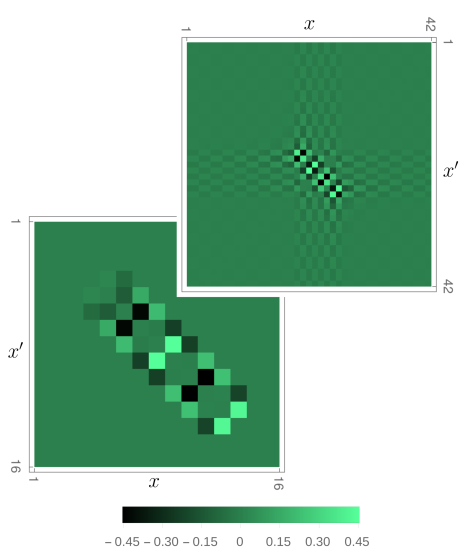
Figure 3: Top: Matrix form of the nonlocal complete polarizer potential. The interaction zone contains different on-site energies indicated by the alternating pixel intensities in the diagonal. Bottom: Matrix form of a geometrical polarizer potential with range $\rho=10$ and no on-site potential. Only couplings to first and second order have been included. Both potentials are given in units of $\Delta$.

III Dynamical study

In this section, we shall study two different phenomena. The first is a “free-particle” effect: Zitterbewegung. Since its proposal by Schrödinger, Zitterbewegung has been understood as a rapid oscillatory motion that is a product of the interference between positive- and negative-energy states present in the initial composition of a Dirac spinor. For this oscillatory phenomena to be observed, these positive- and negative-energy states must have a sufficiently large overlap in position space. This has, in fact, been emulated in other experimental realizations of the Dirac equation Rusin and Zawadzki (2007); Dreisow et al. (2010); Gerritsma et al. (2010). In this work, we develop a clean derivation that will allow us to make a stationary phase approximation leading to a $\sqrt{1/t}$ decay of the oscillatory part of the amplitude. In addition, we shall consider the effect of a designed potential that can spatially separate efficiently a function in its “big” and “small” contribution. The efficiency of the splitter shall be characterized by means of reflection and transmission coefficients for each spin component.

III.1 Wave packet dynamics

Zitterbewegung is the hallmark of unpolarized beams. Effective relativistic wave equations produce oscillatory phenomena in the evolution of single-component spinors on the lattice Dreisow et al. (2010). At the heart of this effect lies the FW picture and the corresponding rotated quasispin: an observable associated to upper and lower energy bands. The outcome of the evolution will be a superposition of ”particles” and ”antiparticles” as long as the initial condition is a mixture of such quantum number. An obvious implication is that Zitterbewegung should be present in any theory with binary lattices. Noteworthy is the fact that the approximation of Bloch momenta around Dirac points is not the essential ingredient; we may find Zitterbewegung in situations where the initial wave packet is a superposition of all energies in both bands, with non-negligible momentum components. We proceed to analyze such physical situations.

Setting $\hbar=1$, we define the initial wave packet as

$$|\psi_{0}\rangle=\int_{0}^{\pi}dk\sum_{s=\pm}\psi_{k,s}|k,s\rangle=\sum_{n}\psi_{n}|n\rangle.$$ (27)

We are interested in the average position at time $t$. In order to recover the usual definition of position $x$ and momentum $p=-i\partial/\partial x$ in the continuous limit, we work with position operators defined over dimers (pairs of sites) and lattice constant $a$,

$$X=\frac{a}{2}\sum_{n\,\mbox{\scriptsize even}}n\left[|n\rangle\langle n|+|n+1\rangle\langle n+1|\right]$$ (28)

with the property

$$\left[T^{2},X\right]=-aT^{2},\qquad\left[X,\sigma_{\pm}\right]=0$$ (29)

(note though that it is the operator $T^{2}$ and not $T$ that satisfies this property). In the Heisenberg picture, we obtain

$$\dot{X}=a\sigma_{2},\qquad\dot{{\bf\Pi}}=0,$$ (30)

which leads to

$$X(t)=X(0)-2at\frac{\Delta\Pi_{2}}{H}\\ +a\left[\sigma_{2}(0)-2\frac{\Delta\Pi_{2}}{H}\right]\int_{0}^{t}dt\,e^{-2itH}.$$ (31)

The first two terms describe the usual classical dynamics for a free particle, while the oscillations (i.e., the Zitterbewegung) come from the third term. The relevant part of the expectation value with respect to the state $|\psi_{0}\rangle$ is thus

$$x_{\rm zitt}\equiv\bigg{\langle}\left[\sigma_{2}(0)-2\frac{\Delta\Pi_{2}}{H}\right]\int_{0}^{t}dt\,e^{-2itH}\bigg{\rangle}_{\psi}.$$ (32)

After inserting energy kets (8) and performing the time integral, we can write

$$x_{\rm zitt}=\sum_{s,s^{\prime}}J_{s,s^{\prime}}+\sum_{s}I_{s}$$ (33)

where $I$ and $J$ are Bloch-momentum integrals of the type

$$J_{s,s^{\prime}}\equiv\int_{0}^{\pi}dk\frac{e^{-iE_{k,s}t}\sin(E_{k,s}t)}{E_{k,s}}\psi_{k,s}\psi^{*}_{k,s^{\prime}}\\ \times i\left[u^{+}_{k,s}(u^{-}_{k,s^{\prime}})^{*}-u^{-}_{k,s}(u^{+}_{k,s^{\prime}})^{*}\right]$$ (34)

and

$$I_{s}\equiv\int_{0}^{\pi}dk\frac{e^{-iE_{k,s}t}\sin(E_{k,s}t)\sin k}{(E_{k,s})^{2}}|\psi_{k,s}|^{2}.$$ (35)

These integrals can be estimated in a long-time regime using the stationary phase approximation, where the stationary points are approximately determined by $dE_{k,s}/dk=0$, i.e., $k=0,\pi/2,\pi$. Since our description involves only $0<k<\pi$, we see that two stationary points lie at the edge of the interval, and therefore their contribution appears with a factor of $1/2$. On the other hand, the midpoint $k=\pi/2$ is also the point of maximal approach between bands, and it only contributes when $\mu\neq 0$. From (34) and (35), we see that $x_{\rm zitt}$ contains terms with a time dependence of the form $e^{i\omega t}\sqrt{1/t}$, after applying the stationary phase approximation. Therefore, the frequencies of oscillation take the values $\omega_{1}=\pm\mu$ (from $k=\pi/2$) and $\omega_{2}=\pm\sqrt{4\Delta^{2}+\mu^{2}}$ (from $k=0,\pi$), while the effect vanishes with an envelope curve $\sqrt{1/t}$. We have an expression of the form

$$x_{\rm zitt}\approx\sqrt{\frac{1}{t}}\left[A(\mu,\Delta)e^{-2i\omega_{1}t}+B(\mu,\Delta)e^{-2i\omega_{2}t}+\mbox{c.c.}\right],$$

(36)

where $A$ and $B$ are coefficients related to second derivatives of the phase in (34) and (35). In Fig. 4, we describe the oscillations of $x_{\rm zitt}$ in log scale, showing clearly an envelope $\sqrt{1/t}$ for long times.

Figure 4: Zitterbewegung of the wave packet. On the left panel, we see the oscillations of $x_{\rm zitt}$ without ballistic motion, as well as the decay of amplitude predicted by stationary phase approximations. On the right panel, we see the same rate of amplitude decay for three different effective masses, $\mu$. $\overline{\Delta x}$ is the averaged maximum amplitude of the oscillations, while $\tau=t/T_{\chi}$ and $T_{\chi}$ is the characteristic time of the simulation given by $T_{\chi}=\hbar/\Delta$.

Figure 5: (Color online) Evolution of a wave packet going through the lattice polarizer. The first picture shows the initial condition of the complete wave packet, whereas the second and third pictures portray the dynamics of the upper and lower band components of the wave packet. The collision time with the polarizer is $T_{c}=\frac{\hbar N}{2\Delta\kappa}$, where $N$ is the number of sites on the lattice.

III.2 The potential as a beam splitter

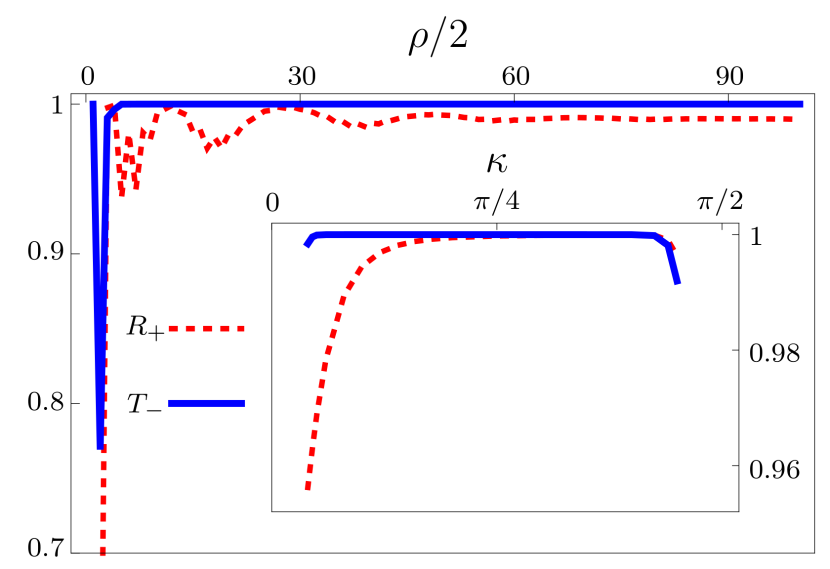
Figure 6: (Color online) The dotted line represents the reflection coefficient for the upper band component of the wave packet as a function of the variables $\kappa$ and the polarizer size $\rho$. The continuous line represents the transmission coefficient for the lower band component of the wave packet as a function of the same variables.

We prepare wave packets with an adjustable width and a proper ”thrust” or ”kick” by means of an additional plane-wave factor, imprinting an average drift. Our choice corresponds to motion from left to right. Eventually, our packets reach the gate keeper centered at the origin described in Fig. 3, but before they do so, Zitterbewegung is significantly observed. After the packets collide with the potential, positive-energy components are reflected and negative-energy components are transmitted. This type of behavior has been verified numerically with specific wave packets, as we discuss now. In Fig. 5, we plot the full probability density in black, upper spin component in blue, and lower spin in orange. The dynamics is described in three steps: the first column corresponds to times before the collision with the polarizer, the second column shows the interference produced by the collision, and the third column finally demonstrates how the components of the wave packet are separated after the collision. Upper spin is reflected and lower spin is transmitted. To make a quantitative analysis in terms of probabilities, first we define the initial wave packet as

$$\psi_{n}(0)=\alpha\mbox{$\cal N\,$}_{-}P_{-}e^{-an^{2}/4\lambda^{2}}e^{i\kappa n}+\beta\mbox{$\cal N\,$}_{+}P_{+}e^{-an^{2}/4\lambda^{2}}e^{-i\kappa n},$$ (37)

where $|\alpha|^{2}+|\beta|^{2}=1$, $\lambda$ is the width of the discrete probability density, and $\kappa$ is the average momentum of the packet. $P_{\pm}$ are the projectors onto each energy band given by

$$P_{s}=\int_{0}^{\pi}dk|k,s\rangle\langle k,s|=U_{FW}\left(\frac{{\bf 1}+s\sigma_{3}}{2}\right)U_{FW}^{\dagger}.$$ (38)

The matrix elements of these projectors are used after the scattering event takes place in the simulation, in order to test the sign of the spin. The results in Fig. 6 show that after our Stern-Gerlach apparatus has done its job, only $1.2\%$ of the upper spin component and $100\%$ of the lower spin component have been transmitted. The wave packet moving to the right still exhibits a slight hint of Zitterbewegung as it is a mixture of components, while the wave packet moving to the left propagates without Zitterbewegung, as it is only comprised by the remainder $98.8\%$ of the upper spin component. This quantitative analysis requires the reflection capacity of the upper spin component, denoted by $R_{+}$, and transmission capacity of the lower spin component, $T_{-}$, of the polarizer for different values of the thrust $\kappa$ and the range of the polarizer $\rho$. These quantities are given by

$$R_{+}=\frac{|P_{+}|\psi(t)\rangle|_{l}^{2}}{|\alpha|^{2}},\quad T_{+}=\frac{|P_{+}|\psi(t)\rangle|_{r}^{2}}{|\alpha|^{2}},\\ R_{-}=\frac{|P_{-}|\psi(t)\rangle|_{l}^{2}}{|\beta|^{2}},\quad T_{-}=\frac{|P_{-}|\psi(t)\rangle|_{r}^{2}}{|\beta|^{2}},$$ (39)

where subscripts $l,r$ stand for sums over sites to the left and right of the polarizer location, respectively. Due to complementarity, $R_{+}+T_{+}=1$ and $R_{-}+T_{-}=1$, so $T_{+}$ and $R_{-}$ are redundant. The results for $R_{+},T_{-}$ are shown in Fig. 6. When $\rho$ is varied, both capacities retain near optimal values and fall to zero only for small polarizer sizes, as expected. Since the ”kick” is a property of the wave packet—i.e., external to the structure of the polarizer—the capacities are expected to remain invariant for different values of $\kappa$. This is confirmed in our simulations, except for values near $\kappa=0,\pi/2$ which correspond to purely diffusive propagation.

The results are quite satisfactory, but we should mention that the type of polarizer ${\bf(}1+\sigma_{3})\otimes V$ could be modified with more refined constructions, even with transparent potentials previously designed using supersymmetric methods Sadurní (2014).

We would like to point out that the inset in Fig. 6 shows the reflection $R_{+}$ rising up very close to 1 for values of $\kappa>\pi/4$ (but far from $\pi/2$). This corresponds to fast wave packets. Since our simulations consist of time-dependent scattering, we need fast and broad distributions that overcome the spreading of components before scattering; we are, however, limited to a finite size of the grid. In addition, our model also allows one to increase the intensity $V$, which blocks incident beams with increasing efficiency as long as $\kappa$ does not correspond to a Ramsauer resonance.

III.3 A purely geometric beam splitter

Engineering beam splitters by means of nonlocal potentials include the possibility of removing all diagonal contributions in $V$, in favor of the off-diagonal elements representing interactions to a certain range, as shown in Fig. 3 (our approximations may include nearest neighbors, next-to-nearest neighbors, and so on). In the experimental setup to be described in later sections, the couplings can be determined by proximity between sites. With this technique, we can control the interaction range, as well as the zone where it operates, only using lattice deformations. Wave-packet evolution is studied numerically in this extreme situation and our results show a surprisingly efficient separation of components. In particular, for a $\rho=10$ polarizer with couplings to second-order neighbors, we see a reflection of $67.9\%$ of the upper spin component and a transmission of $92.6\%$ of the lower spin component.

IV Feasibility

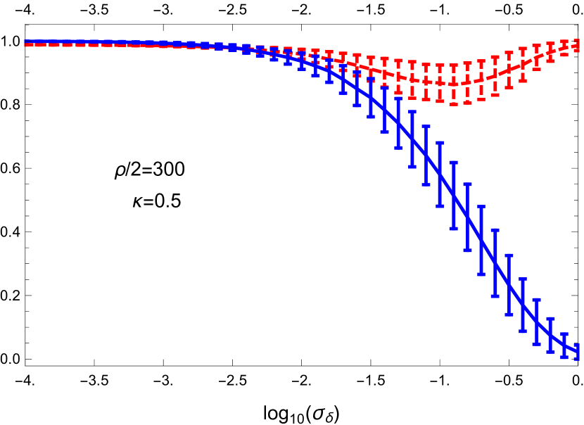
Figure 7: (Color online) Mean reflection (red) and transmission (blue) coefficients as functions of the standard deviation of the coupling $\sigma_{\delta}$ (see text), for a $\rho=600$ splitter. The error bars represent the fluctuations obtained from multiple realizations. The value $\kappa=0.5$ has been chosen for optimality.

In this section, we test the robustness of the splitter with respect to the known experimental limitations. In the splitter, three parameters must be controlled: the overall absorption, the on-site energy, and the coupling terms. This analysis will not include the overall absorption because it mainly affects the width and height of the resonances without significantly disturbing the spectral positions; therefore, it is expected that the transmission and reflection coefficients decrease by a factor related to the strength of the absorption.
Experiments show Bellec et al. (2013) that the on-site energy can be controlled better than the coupling. This is the case for microwave experiments since the variation of couplings is at least two orders of magnitude greater than the variation of the on-site energy. Thus, to estimate the robustness of the splitter, we will consider a Gaussian disorder introduced randomly on the couplings. We modify $\Delta\rightarrow(1-\delta)\Delta$, where $\delta$ is a random variable with a standard deviation $\sigma_{\delta}$. Figure 7 shows that the expected coefficients and deviations are satisfactory, even for a poor coupling control ($\sigma_{\delta}\sim 0.1$). As expected, an extremely poor coupling control ($\sigma_{\delta}\gg 0.1$) destroys the efficiency of the splitter, with the latter becoming a regular wall unable to separate the upper and lower band components. Thus, we have shown robustness and feasibility in laboratory implementations.

V Experimental proposals

In this section, we describe a realization of the splitter through a microwave cavity containing a set of cylindrical resonators between parallel plates, establishing a tight-binding configuration. This type of experimental implementation has been very useful for the emulation of Dirac equations Franco-Villafañe et al. (2013), graphenelike structures Bittner et al. (2010); Kuhl et al. (2010); Barkhofen et al. (2013); Bellec et al. (2013), chiral states Dembowski et al. (2003), and anomalous Anderson localization Fernández-Marín et al. (2014), among others. It is important to mention that the following experimental proposal is not unique since the splitter can also be achieved by plasmonic circuits Martínez-Galera et al. (2014), optical waveguides Longhi (2009), or acoustic waves Maynard (2001). The reader can notice that these implementations rely on classical aspects of the systems mentioned. However, the equations of motion are equivalent to, say, the Schrödinger or Dirac’s equation, depending on the regime studied. In this sense, we are emulating Dirac’s equation.

We show in further detail how to produce complex coupling constants with the aim of fabricating purely geometric beam splitters. The effect, important in its own right, rests on the possibility of breaking the chiral symmetry of polygonal geometries using dimers as individual sites. This opens the possibility of producing directed couplings, emerging from dimeric states.

V.1 Experimental specifications

A set of cylindrical dielectric disks can act as the sites of the chain, for example, Temex-Ceramics disks, E2000 series, with high dielectric permittivity ($\epsilon=37$) and low loss (quality factor $Q=7000$). Each disk has an isolated resonance defined by the dimensions of the cylinder, e.g., for a height of $5$mm and a radius of $4$mm, a resonance close to 6.64 GHz appears corresponding to the lowest transverse electric mode (TE₁). This resonant frequency is equivalent to the on-site energy. For purely geometric splitters, we have seen that on-site energies are the same throughout the array; therefore, identical dielectric disks must be used. On the other hand, a general type of splitter would require disks of different dimensions and/or dielectric constants.

Between two parallel metallic plates, each isolated resonance behaves like a $J_{0}$-Bessel function inside of a cylinder, and as a $K_{0}$-Bessel function outside of it. The function $K_{0}$ can be represented fairly well by an exponential tail as a function of the distance with respect to the center. Therefore, any set of disks interacts by proximity through the overlap of their individual functions $K_{0}$, in such a way that the response of the whole set is well described by a tight-binding model. The intensity of the interaction and the main contribution of first and second neighbors can be further manipulated by changing the distance between the plates Sadurní et al. (2013).

It is possible to study the wave dynamics of the splitter by introducing two antennas into the microwave cavity connected to different ports of a vector network analyzer (VNA). It is possible to measure both the spectrum and the intensity of the wave functions by using only one probing antenna. However, for the reconstruction of wave packet dynamics, it is necessary not only to measure the intensity but also the phase. Hence a second antenna probing the transmission of the system is mandatory.

We fix one of the antennas near to a disk whereby the electromagnetic waves are injected, while the position of the other antenna is varied throughout the structure, allowing one to measure the transmission spectrum on each disk.

The evolution of the wave packet at each point of the structure is reconstructed through a Fourier transform of the measured spectrum at that point Böhm et al. (2015). This is allowed because we have access to the full spectrum of the complex transmission.

V.2 Negative couplings and level inversion

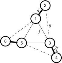
Figure 8: Configuration of disks (indicated as circles, with a number) giving rise to the coupling structure specified by Eq. (43). The six disks are organized in pairs $(1,2)$, $(3,4)$, and $(5,6)$, each of which interacts strongly via the coupling constant $d$. The inner disks interact via the coupling constant $f$. The outer disks interact with just one of the other four disks (for example, 2 with 3), as the others remain screened geometrically. The $C_{3v}$ symmetry is broken by tilting the outer disks with an angle $\theta$.

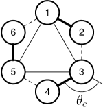
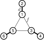
Figure 9: Two particular realizations that keep the full $C_{3v}$ symmetry are illustrated, one in which $\theta=\theta_{c}$, and the other for $\theta=0$ in which screening sets $g=0$.

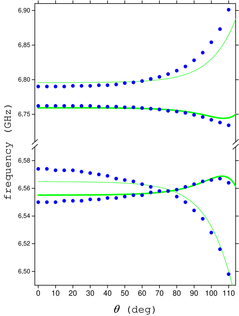
Figure 10: Spectrum of the configuration shown in Fig. 8; dots correspond to a full 3D simulation of a microwave cavity using COMSOL 5.2 and continuous lines correspond to tight-binding calculations. The lower band shows the desired inversion level due to effective negative coupling.

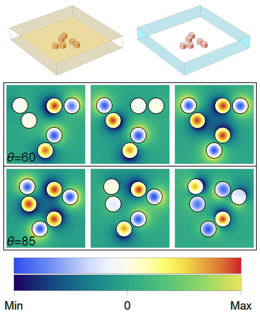
Figure 11: Upper row: simulated 3D system; dielectric disks depicted in light brown, nonreflective walls in cyan, and perfect conductors in yellow. Lower row: lowest modes for $\theta=60$ (before level inversion) and $\theta=85$ (after level inversion). Two different scales have been used inside and outside the cylinders for better visibility. The wave functions outside the cylinders exhibit the nature of couplings.

In our purely geometric splitter, we find matrix elements that are real but not positive; see, e.g., Fig. 3. Negative couplings require the control of an extra degree of freedom in the form of a phase factor. We show that indeed such phases can be produced by adding more structure in our arrays. It is worth mentioning that nonremovable phase factors in hopping amplitudes are the equivalent of magnetic fields applied to charged particles Hofstadter (1976), but our goal is to emulate these effects for a scalar wave.

First we note that any Hermitian matrix $H$ can be rewritten as a matrix with semipositive secondary diagonals by means of a unitary transformation. We proceed to turn $H$ into a purely positive nearest-neighbor array. Consider

$$U_{\mbox{\scriptsize sign}}=\mbox{diag}\left\{e^{-i\Delta_{n}}\right\},$$ (40)

where $\Delta_{n}=\sum_{m<n}\arg H_{m+1,m}$ is the accumulated phase of the elements in the first diagonal. This trivial ”gauge” transformation moves all possible phases to third diagonals or next-to-nearest neighbors; we must now analyze the influence of sign flips in the hopping amplitudes. The zigzag arrays shown in Fig. 2 are made of alternating triangular blocks; therefore, every negative sign occurring in our polarizer corresponds to those bonds lying on the outer part of the array (see Fig. 2). For this reason, we focus on a single triangular block.

The effect of a negative matrix element in this case produces level inversion, as shown by the Hamiltonians

$$H^{\pm}_{\mbox{\scriptsize Block}}=\left(\begin{array}[]{ccc}E_{0}&\Delta&\pm\Delta\\ \Delta&E_{0}&\Delta\\ \pm\Delta&\Delta&E_{0}\end{array}\right)$$ (41)

which are related by the unitary transformation $U_{\mbox{\scriptsize Block}}=\mbox{diag}\left\{-1,1,-1\right\}$ in the form

$$U_{\mbox{\scriptsize Block}}H^{-}_{\mbox{\scriptsize Block}}U_{\mbox{\scriptsize Block}}^{\dagger}=2E_{0}-H^{+}_{\mbox{\scriptsize Block}}.$$ (42)

This compels one to consider each triangular block on the polarizer as a level-inverting interaction. The simplest way to produce a level-inverted band is by the introduction of dimers instead of single-resonance sites; see Fig. 8.

In the ideal situation where only a change of sign is intended, the dimers are placed such that the $C_{3}$ symmetry of the array is not destroyed. To this end, the orientation of the dimers must be constrained, as shown in Fig. 9. Note, however, that the full symmetry of an equilateral triangle $C_{3v}$ is now, in general, broken. The resulting shapes are hexagonal variants described by the following tight-binding matrix:

$$\left(\begin{array}[]{cccccc}0&d&f&0&f&g\\ d&0&g&0&0&0\\ f&g&0&d&f&0\\ 0&0&d&0&g&0\\ f&0&f&g&0&d\\ g&0&0&0&d&0\end{array}\right).$$ (43)

The spectrum contains two degenerate doublets and two singlets. Moreover, their eigenfrequencies are symmetrically disposed around $E_{0}$. In essence, we have produced an additional inverted copy of the spectrum due to a splitting caused by strong intradimer coupling. For dielectric disks, a numerical simulation of Maxwell equations with space-dependent dielectric functions has been run. The results in Fig. 10 show that the inverted copy corresponds to eigenfrequencies sitting to the left of the original isolated resonance at $E_{0}$. Moreover, this occurs only for $\theta>\theta_{c}\sim 78$ deg, which establishes the existence of a diabolic (crossing) point in the spectrum Berry (1984). Transverse modes are shown in Fig. 11, where the panels exhibit a change in the sign of the wave function inside at least one dimer, due to the transition at $\theta_{c}$.

Finally, our results show that the assembled structure of alternating triangles must produce two bands opening around each level of a single dimer: we may choose to work in one or the other. A similar spectral structure has been achieved in other contexts: nuclear resonances von Brentano and Philipp (1999), flat microwave cavities Dembowski et al. (2001); Bittner et al. (2014), and electronic circuits Stehmann et al. (2004).

VI Conclusion and outlook

In this paper, we have studied a tight-binding model that is described by a Dirac equation. We have focused on the time-dependent dynamics in the positive- and negative-energy bands. In the language of the Dirac equation, this corresponds to particles and antiparticles. We have developed the theory that allows one to split these components by means of a localized potential; this in turn could be a first step towards the actual measurement of quasispin using wave packets. We have further shown that even though the interactions are long ranged, taking as few as next-to-nearest-neighbor interactions, in a very localized region in space, yields reasonable results. In connection with the possibility of generating pure spin waves with our splitter, we would like to add that waves with vanishing average momentum have been achieved and that quasispin can be indeed spatially transported. However, the mechanism relies on deformations rather than the application of external magnetic fields as in the usual case of spin. The local nature of the interaction is highly desirable if an experimental emulation is pursued. We have indeed explored such scenario in the context of a bidimensional array of dielectrics in a microwave cavity. In such an array, it has been necessary to consider level inversion, which we have demonstrated using a simple geometric array. The next obvious step would be to carry out the experiment.

*

Appendix A An alternative splitter

A simple alternative splitter can be designed if we replace Eq. (17) by

$$V_{\pm}(x)=\begin{cases}V(x)&\text{for particles}\\ -V(x)&\text{for holes}\end{cases}.$$ (44)

Then, Hamiltonian (18) would be replaced by

$$\tilde{H}_{\mbox{\scriptsize FW}}=H_{\mbox{\scriptsize FW}}+\sigma_{3}\otimes V_{\mbox{\scriptsize FW}}.$$ (45)

In formula (20), one would need an extra term,

$$V_{11}=e^{-i\phi/2}\cos\left(\frac{\theta}{2}\right)V_{\mbox{\scriptsize FW}}\cos\left(\frac{\theta}{2}\right)e^{i\phi/2}\\ +e^{-i\phi/2}\sin\left(\frac{\theta}{2}\right)V_{\mbox{\scriptsize FW}}\sin\left(\frac{\theta}{2}\right)e^{i\phi/2},$$ (46)

which leads to the following changes in the matrix elements:

$$\langle n|V_{11}|n^{\prime}\rangle=\frac{1}{8\pi^{2}}\sum_{m=-\infty}^{\infty}V_{\mbox{\scriptsize FW}}(m)\\ \times\left[I_{n^{\prime}-m}^{++}\left(I_{n-m}^{++}\right)^{*}+I_{n^{\prime}-m}^{--}\left(I_{n-m}^{--}\right)^{*}\right],$$ (47)

for even $n$ and $n^{\prime}$,

$$\langle n|V_{21}|n^{\prime}\rangle=\frac{1}{8\pi^{2}}\sum_{m=-\infty}^{\infty}V_{\mbox{\scriptsize FW}}(m)\\ \times\left[I_{n^{\prime}-m}^{--}\left(I_{n-m}^{+-}\right)^{*}-I_{n^{\prime}-m}^{++}\left(I_{n-m}^{-+}\right)^{*}\right],$$ (48)

for even $n$ and odd $n^{\prime}$, and, finally,

$$\langle n|V_{22}|n^{\prime}\rangle=\frac{1}{8\pi^{2}}\sum_{m=-\infty}^{\infty}V_{\mbox{\scriptsize FW}}(m)\\ \times\left[I_{n^{\prime}-m}^{-+}\left(I_{n-m}^{-+}\right)^{*}+I_{n^{\prime}-m}^{+-}\left(I_{n-m}^{+-}\right)^{*}\right],$$ (49)

for odd $n$ and $n^{\prime}$.

References

- Morsch and Oberthaler (2006) O. Morsch and M. K. Oberthaler, Rev. Mod. Phys. 78, 179 (2006).
- Bloch (2005) I. Bloch, Nat. Phys. 1, 23 (2005).
- Oberthaler et al. (1996) M. K. Oberthaler, R. Abfalterer, S. Bernet, J. Schmiedmayer, and A. Zeilinger, Phys. Rev. Lett. 77, 4980 (1996).
- Uehlinger et al. (2013) T. Uehlinger, G. Jotzu, M. Messer, D. Greif, W. Hofstetter, U. Bissbort, and T. Esslinger, Phys. Rev. Lett. 111, 185307 (2013).
- Struck et al. (2012) J. Struck, C. Ölschläger, M. Weinberg, P. Hauke, J. Simonet, A. Eckardt, M. Lewenstein, K. Sengstock, and P. Windpassinger, Phys. Rev. Lett. 108, 225304 (2012).
- Kuhl et al. (2010) U. Kuhl, S. Barkhofen, T. Tudorovskiy, H.-J. Stöckmann, T. Hosain, L. de Forges de Parny, and F. Mortessagne, Phys. Rev. B 82, 094308 (2010).
- Barkhofen et al. (2013) S. Barkhofen, M. Bellec, U. Kuhl, and F. Mortessagne, Phys. Rev. B 87, 035101 (2013).
- Bittner et al. (2010) S. Bittner, B. Dietz, M. Miski-Oglu, P. Oria-Iriarte, A. Richter, and F. Schäfer, Phys. Rev. B 82, 014301 (2010).
- Bellec et al. (2013) M. Bellec, U. Kuhl, G. Montambaux, and F. Mortessagne, Phys. Rev. B 88, 115437 (2013).
- Martínez-Galera et al. (2014) A. J. Martínez-Galera, I. Brihuega, A. Gutiérrez-Rubio, T. Stauber, and J. M. Gómez-Rodríguez, Sci. Rep. 4, 7314 (2014), arXiv:1411.5805 [cond-mat.mes-hall] .
- Polini et al. (2013) M. Polini, F. Guinea, M. Lewenstein, H. C. Manoharan, and V. Pellegrini, Nat. Nanotechnol. 8, 625 (2013).
- Gomes et al. (2012) K. K. Gomes, W. Mar, W. Ko, F. Guinea, and H. C. Manoharan, Nature 483, 306 (2012).
- Semenoff (1984) G. W. Semenoff, Phys. Rev. Lett. 53, 2449 (1984).
- Geim and Novoselov (2007) A. K. Geim and K. S. Novoselov, Nat. Mater. 6, 183 (2007).
- Neto et al. (2009) A. H. C. Neto, F. Guinea, N. M. R. Peres, K. S. Novoselov, and A. K. Geim, Rev. Mod. Phys. 81, 109 (2009).
- Roati et al. (2007) G. Roati, M. Zaccanti, C. D’Errico, J. Catani, M. Modugno, A. Simoni, M. Inguscio, and G. Modugno, Phys. Rev. Lett. 99, 010403 (2007).
- Fallani et al. (2007) L. Fallani, J. E. Lye, V. Guarrera, C. Fort, and M. Inguscio, Phys. Rev. Lett. 98, 130404 (2007).
- Franco-Villafañe et al. (2013) J. A. Franco-Villafañe, E. Sadurní, S. Barkhofen, U. Kuhl, F. Mortessagne, and T. H. Seligman, Phys. Rev. Lett. 111, 170405 (2013).
- Sadurní et al. (2013) E. Sadurní, J. A. Franco-Villafañe, U. Kuhl, F. Mortessagne, and T. H. Seligman, New J. Phys. 15, 123014 (2013).
- Sadurní et al. (2010) E. Sadurní, T. H. Seligman, and F. Mortessagne, New J. Phys. 12, 053014 (2010).
- Mancini et al. (2015) M. Mancini, G. Pagano, G. Cappellini, L. Livi, M. Rider, J. Catani, C. Sias, P. Zoller, M. Inguscio, M. Dalmonte, and L. Fallani, Science 349, 1510 (2015).
- Wilczek (2009) F. Wilczek, Nat. Phys. 5, 614 (2009).
- Alicea (2012) J. Alicea, Rep. Prog. Phys. 75, 076501 (2012).
- Kagalovsky et al. (1999) V. Kagalovsky, B. Horovitz, Y. Avishai, and J. T. Chalker, Phys. Rev. Lett. 82, 3516 (1999).
- Bernard and LeClair (2001) D. Bernard and A. LeClair, Phys. Rev. B 64, 045306 (2001).
- Dreisow et al. (2010) F. Dreisow, M. Heinrich, R. Keil, A. Tünnermann, S. Nolte, S. Longhi, and A. Szameit, Phys. Rev. Lett. 105 (2010).
- Meier et al. (2007) L. Meier, G. Salis, I. Shorubalko, E. Gini, S. Schön, and K. Ensslin, Nat. Phys. 3, 650 (2007).
- Foldy and Wouthuysen (1950) L. L. Foldy and S. A. Wouthuysen, Phys. Rev. 78, 29 (1950).
- Vries (1970) E. D. Vries, Fortschr. Phys. 18, 149 (1970).
- Rusin and Zawadzki (2007) T. M. Rusin and W. Zawadzki, Phys. Rev. B 76, 195439 (2007).
- Gerritsma et al. (2010) R. Gerritsma, G. Kirchmair, F. Zahringer, E. Solano, R. Blatt, and C. F. Roos, Nature 463, 68 (2010).
- Sadurní (2014) E. Sadurní, Phys. Rev. E 90, 033205 (2014).
- Dembowski et al. (2003) C. Dembowski, B. Dietz, H.-D. Gräf, H. L. Harney, A. Heine, W. D. Heiss, and A. Richter, Phys. Rev. Lett. 90 (2003).
- Fernández-Marín et al. (2014) A. A. Fernández-Marín, J. A. Méndez-Bermúdez, J. Carbonell, F. Cervera, J. Sánchez-Dehesa, and V. A. Gopar, Phys. Rev. Lett. 113, 233901 (2014).
- Longhi (2009) S. Longhi, Laser & Photon. Rev. 3, 243 (2009).
- Maynard (2001) J. D. Maynard, Rev. Mod. Phys. 73, 401–417 (2001).
- Böhm et al. (2015) J. Böhm, M. Bellec, F. Mortessagne, U. Kuhl, S. Barkhofen, S. Gehler, H.-J. Stöckmann, I. Foulger, S. Gnutzmann, and G. Tanner, Phys. Rev. Lett. 114 (2015).
- Hofstadter (1976) D. R. Hofstadter, Phys. Rev. B 14, 2239 (1976).
- Berry (1984) M. V. Berry, Proc. R. Soc. Lond. A 392, 45 (1984).
- von Brentano and Philipp (1999) P. von Brentano and M. Philipp, Phys. Lett. B 454, 171 (1999).
- Dembowski et al. (2001) C. Dembowski, H.-D. Gräf, H. L. Harney, A. Heine, W. D. Heiss, H. Rehfeld, and A. Richter, Phys. Rev. Lett. 86, 787 (2001).
- Bittner et al. (2014) S. Bittner, B. Dietz, H. L. Harney, M. Miski-Oglu, A. Richter, and F. Schäfer, Phys. Rev. E 89 (2014).
- Stehmann et al. (2004) T. Stehmann, W. D. Heiss, and F. G. Scholtz, J. Phys. A 37, 7813 (2004).